Profile Likelihood via Optimisation and Differential Equations

Abstract

Profile likelihood provides a general framework to infer on a scalar parameter of a statistical model. A confidence interval is obtained by numerically finding the two abscissas where the profile log-likelihood curve intersects an horizontal line. An alternative derivation for this interval can be obtained by solving a constrained optimisation problem which can broadly be described as: maximise or minimise the parameter of interest under the constraint that the log-likelihood is high enough. This formulation allows nice geometrical interpretations; It can be used to infer on a parameter or on a known scalar function of the parameter, such as a quantile. Widely available routines for constrained optimisation can be used for this task, as well as Markov Chain Monte Carlo samplers. When the interest is on a smooth function depending on an extra continuous variable, the constrained optimisation framework can be used to derive Ordinary Differential Equation (ODE) for the confidence limits. This is illustrated with the return levels of Extreme Value models based on the Generalised Extreme Value distribution. Moreover the same ODE-based technique applies as well to the derivation of profile likelihood contours for couples of parameters. The initial value of the ODE used in the determination of the interval or the contour can itself be obtained by another auxiliary ODE with known initial value obtained by using the confidence level as the extra continuous variable.

^⋆Statistical Consultant, Chambéry FR.
Email: deville.yves@alpestat.com.

1 Problem

We consider here a regular parametric statistical model depending on a vector $\boldsymbol{\theta}$ of $p$ parameters, and focus on the inference on a specific scalar component of the parameter using a vector of observations $\mathbf{y}$, possibly depending on covariates. Without loss of generality we focus on the first component denoted by $\psi$, while $\boldsymbol{\lambda}$ will be the vector of the remaining $p-1$ components, so $\boldsymbol{\theta}=[\psi,\,\boldsymbol{\lambda}^{\top}]^{\top}$. The log-likelihood function $\ell(\boldsymbol{\theta};\,\mathbf{y})$ will be denoted as $\ell(\boldsymbol{\theta})$ or $\ell(\psi,\,\boldsymbol{\lambda})$ and will be assumed to be differentiable twice at least. We will assume that the log-likelihood is “well-shaped”: it has a unique maximum $\hat{\boldsymbol{\theta}}$ with components $\hat{\psi}$ and $\hat{\boldsymbol{\lambda}}$, and moreover the profile log-likelihood denoted by $\ell_{\texttt{prof}}(\psi)$ will be assumed to be increasing in $\psi$ for $\psi\leqslant\hat{\psi}$, and to be decreasing for $\psi\geqslant\hat{\psi}$. We denote somewhat abusively by $\psi(\boldsymbol{\theta})$ and $\boldsymbol{\lambda}(\boldsymbol{\theta})$ the sub-vectors of $\boldsymbol{\theta}$ with respective length $1$ and $p-1$.

Using our assumption that the log-likelihood is well-shaped, we can denote by $\psi_{\texttt{U}}$ the upper bound of the likelihood-profile confidence interval with level $1-\alpha$. The value $\psi_{\texttt{U}}>\hat{\psi}$ is a solution of the equation

$$\ell_{\texttt{prof}}(\psi)=\ell_{\max}-\delta$$ (1)

where $\ell_{\max}=\ell(\hat{\boldsymbol{\theta}})$ is the maximal log-likelihood, and where $\delta>0$ relates to the quantile of the $\chi^{2}$ distribution with one degree of freedom according to $\delta=q_{\chi^{2}(1)}(1-\alpha)/2$. Similarly the lower bound $\psi_{\texttt{L}}$ solves the equation (1) with $\psi_{\texttt{L}}<\hat{\psi}$, see Figure 1. The specific choice of $\delta$ grants that the confidence interval asymptically reaches the prescribed confidence level.

Figure 1: Profile likelihood interval in the “well-shaped” case.

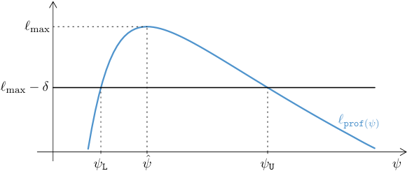
The practical determination of profile likelihood intervals can rely on what we may call a naive method: the profile likelihood function $\ell_{\texttt{prof}}(\psi)$ being implemented by using a numerical $(d-1)$-dimensional optimisation, one can solve (1) by using a zero-finding method. Venzon and Moolgavkar (1988) instead designed an algorithm to find the bounds of the confidence interval by solving a nonlinear equation in $\boldsymbol{\theta}$, hence without computing the profile likelihood as such. Quite recently, some authors have designed implementations of the profile likelihood inference by relying on a formulation as a constrained optimisation problem in which the objective is the parameter of interest, realising that the non-linear equation used by Venzon and Moolgavkar encodes the Karush-Kuhn-Tucker conditions for this optimisation problem. While this potentially makes the use of the profile likelihood method nearly as simple as that of the cheap delta method, practical problems arise related to the optimisation. Fisher and Lewis (2021) have designed a dedicated optimisation algorithm called RVM for Revised Venzon-Moolgavkar. They have studied a variety of strategies regarding the numerical optimisation and have found that the RVM outperforms the original Venzon-Moolgavkar method and the other methods on a large benchmark of problems. Borisov and Metelkin (2020) also describe the use of optimisation in a software computing profile likelihood confidence intervals on a parameter or on a function of the parameter vector. They discuss the question of practical identifiability in relation with a specific form of model as used in biology.

Our motivation is for models related to the Extreme Value (EV) theory, such as models for block maxima, with margins following the Generalised Extreme-Value (GEV) distribution. For these models, the confidence intervals based on profile likelihood are known to have a much better coverage rate than those based on the delta method or on the bootstrap. We will focus on the use of the R language (R Core Team 2022) for the implementation. In practice, the profile likelihood intervals are often computed via the naive method as is the case for the famous R packages available on the Comprehensive R Archive Network (CRAN): ismev (Stephenson and Heffernan 2018), evd (Stephenson 2002), extRemes (Gilleland and Katz 2016), mev (Belzile 2023) and others. Beside the model parameters, one often has to infer on the return levels corresponding to large return periods such as $100$ or even $1000$ years, and some tedious re-parameterisation can then be required. For EV models, a Bayesian predictive approach is nowadays often preferred to the frequentist approach since it provides more easily interpreted results and eventually avoids the use of return levels. However the likelihood inference has the advantage of being independent of the specific parameterisation used, which is not the case for the Bayesian inference, even when a non-informative prior is used. To our best knowledge, using constrained optimisation methods for the inference on EV models has not yet been reported. We have been experimenting on this for several years and came up to some methods relying on the use of Ordinary Differential Equation (ODE) as described in sections 4 and 5

This paper is organised as follows. In section 2 we recall the constrained optimisation formulation. In section 3 we focus on the inference on a function of the parameter, illustrate it on examples and discuss some practical issues. In Section 4 we consider a function depending on an extra “time” variable and show how an ODE then naturally arises. Section 5 describes some methods closely related to the geometry of the profile likelihood contours or of the likelihood contours: ODEs can be used in relation with a suitable time variable with geometrical interpretation. Finally, Section 6 and discusses on limitations and possible extensions.

2 Optimisation problems

The profile log-likelihood function $\ell_{\texttt{prof}}(\psi)$ is defined by

$$\ell_{\texttt{prof}}(\psi):=\ell\{\psi,\,\hat{\boldsymbol{\lambda}}(\psi)\}$$ (2)

where $\hat{\boldsymbol{\lambda}}(\psi)$ maximises the function $\boldsymbol{\lambda}\mapsto\ell(\psi,\,\boldsymbol{\lambda})$. So for a given $\psi$, the vector $[\psi,\,\hat{\boldsymbol{\lambda}}(\psi)^{\top}]^{\top}$ is the solution of an optimisation problem with equality constraint

$$\underset{\boldsymbol{\theta}}{\textrm{maximise}} \ell(\boldsymbol{\theta})$$ (3)

subject to $$\psi(\boldsymbol{\theta})=\psi.$$

With the assumptions above, we can regard the upper bound $\psi_{\texttt{U}}$ of the confidence interval on $\psi$ as the solution of

$$\underset{\psi}{\text{maximise}} \psi$$ (4)

subject to $$\ell_{\texttt{prof}}(\psi)\geqslant\ell_{\max}-\delta.$$

Indeed, $\psi_{\texttt{U}}$ is the largest $\psi$ for which the inequality $\ell_{\texttt{prof}}(\psi)\geqslant\ell_{\max}-\delta$ holds. The constraint function of this problem is itself defined as the solution of an optimisation problem, which limits its practical use. Yet we can instead solve the following optimisation problem which uses the log-likelihood function as constraint function.

Proposition 1.

Let $\psi^{\star}$ be defined as $\psi(\boldsymbol{\theta}^{\star})$ where $\boldsymbol{\theta}^{\star}$ with components $\psi^{\star}$ and $\boldsymbol{\lambda}^{\star}$ is the solution of the constrained optimisation problem

$$\underset{\boldsymbol{\theta}}{\text{maximise}} \psi(\boldsymbol{\theta})$$ (5)

subject to $$\ell(\boldsymbol{\theta})\geqslant\ell_{\max}-\delta,$$

where $\delta:=q_{\chi^{2}(1)}(1-\alpha)/2$. Then $\psi^{\star}$ is nothing but the upper end-point $\psi_{\texttt{U}}$ of the $100(1-\alpha)\%$ confidence interval obtained by profile likelihood. Similarly, if $\boldsymbol{\theta}_{\star}$ with components $\psi_{\star}$ and $\boldsymbol{\lambda}_{\star}$ is the solution of the minimisation of $\psi(\boldsymbol{\theta})$ under the same constraint, then $\psi_{\star}$ is the lower bound $\psi_{\texttt{L}}$ of the profile likelihood confidence interval.

A proof for this simple result is given in Appendix A. An appealing geometrical derivation for the case $p=2$ is as follows. The profile log-likelihood for $\psi$ is the profile of a surface in the usual meaning, namely the log-likelihood surface. This profile is the curve that would be seen by an observer located at infinity in the direction of the $\lambda$-axis, at $\lambda=-\infty$. By cutting the surface at the level $\ell_{\max}-\delta$ we define a contour projecting on the $\psi\lambda$-plane into the contour of the feasible set, say $\mathcal{R}(\delta)$, of problem (5). Obviously, our observer can locate $\psi_{\texttt{L}}$ and $\psi_{\texttt{U}}$ as the value of $\psi$ for the leftmost and the rightmost point that can be seen in $\mathcal{R}$. These are identical to the values where the profile is seen to cut the horizontal line corresponding to the altitude $\ell_{\max}-\delta$.

Remark 1.

Suppose that the ML estimate is available in closed form for one component of $\boldsymbol{\lambda}$, for instance $\lambda_{1}$. Then in the optimisation problem (5) we can replace the vector $\boldsymbol{\theta}$ by the vector $\boldsymbol{\theta}_{\lambda_{1}^{\text{c}}}$ with length $p-1$ obtained by discarding $\lambda_{1}$ from $\boldsymbol{\theta}$ and replace the log-likelihood $\ell(\boldsymbol{\theta})$ in the constraint by the profile likelihood function $\ell_{\lambda_{1}^{\text{c}}}(\boldsymbol{\theta}_{\lambda_{1}^{\text{c}}})$ obtained from $\ell(\boldsymbol{\theta})$ by replacing $\lambda_{1}$ by its ML estimate $\hat{\lambda}_{1}(\boldsymbol{\theta}_{\lambda_{1}^{\text{c}}})$. The main point here is that the objective $\psi(\boldsymbol{\theta})=\psi$ does not depend on $\lambda_{1}$. An example will be given in section 3.3 below.

Remark 2.

In the constraint of (5) the equality $\ell(\boldsymbol{\theta})=\ell_{\max}-\delta$ can be used in place of the inequality.

3 Function of the parameter vector

3.1 Function value vs. parameter

In many situations we want to infer on a scalar smooth function of the parameter vector, say $\eta(\boldsymbol{\theta})$. A typical example is when $\eta$ is the expectation of a response for some “new” value of a vector of covariates. The profile likelihood method can then be used.

An usual approach is to consider $\eta(\boldsymbol{\theta)}$ as a scalar parameter using a suitable re-parameterisation of the model that discards one the original parameters and replaces it by $\eta$. Mathematical conditions for the existence of such a re-parameterisation seem quite complex and will not be discussed here. Yet if this re-parameterisation is admissible, we are exactly in the situation of the previous sections with $\psi(\boldsymbol{\theta})$ replaced by $\eta(\boldsymbol{\theta})$.

There are some difficulties in the previous approach. Needless to say, a careful analysis is required to choose the discarded parameter. From a software engineering point of view, this can be tedious because models are often defined using formulas, and these are not easily re-parameterised. The re-parameterisation can also have a negative impact on the numerical conditioning e.g., when the new parameter turns out to be strongly correlated to those kept in the model. Moreover, the interest can be both on the parameters and on a function of these, or on several functions of the parameters: Using a regression model, several predictions are often considered. With several functions, we have to use as many re-parameterisations. By contrast, it is much simpler to rely on Proposition 1 and use an optimisation program with the objective function being $\eta(\boldsymbol{\theta})$ instead of $\psi(\boldsymbol{\theta})$. A constrained optimisation algorithm should perform automatically a good local re-parameterisation based on the value of the iterate, and this is likely to work better than the global re-parametrisation considered above.

An approximate confidence region $\mathcal{R}$ on the the full parameter vector $\boldsymbol{\theta}$ is obtained as

$$\mathcal{R}(\delta):=\left\{\boldsymbol{\theta}:\,\ell(\boldsymbol{\theta})\geqslant\ell_{\max}-\delta\right\}$$ (6)

with $\delta:=q_{\chi^{2}(p)}(1-\alpha)/2$. Quite obviously, a so-called conservative confidence interval on $\eta$ can be obtained by minimising and maximising $\eta(\boldsymbol{\theta})$ for $\boldsymbol{\theta}\in\mathcal{R}$ to get the confidence limits $\eta_{\texttt{L}}$ and $\eta_{\texttt{U}}$. A striking point is that Prop. 1 tells that we can replace in the definition of $\delta$ the quantile $q_{\chi^{2}(p)}$ of the $\chi^{2}$ distribution with $p$ degree of freedom by the equivalent quantile $q_{\chi^{2}(1)}$ for one degree of freedom (d.f.), leading to a much smaller confidence interval. An essential point is that $\eta(\boldsymbol{\theta})$ must be such that it can be used as a parameter for the model; This is a condition of identiability.

In the Bayesian framework, the inference on a function of the parameter, be it scalar or vector, is straightforward. Indeed if Monte Carlo Markov Chain (MCMC) iterates $\boldsymbol{\theta}^{[k]}$ are available, the values $\eta(\boldsymbol{\theta}^{[k]})$ can be computed to provide a sample of the posterior distribution for $\eta(\boldsymbol{\theta})$. Credible intervals on $\eta(\boldsymbol{\theta})$ can then be given. However, a prior for $\boldsymbol{\theta}$ is involved in this process. By using a non-informative “flat” prior with $p(\boldsymbol{\theta})\propto 1$ (most often improper), the posterior density will be proportional to the likelihood. Yet the prior for $\boldsymbol{\theta}$ induces a prior for $\eta(\boldsymbol{\theta})$ which may be informative, especially when the available observations carry little information about $\eta(\boldsymbol{\theta})$. An example is provided by a regression model when $\eta(\boldsymbol{\theta})$ is a new response at a design point far away from the design points used in the fit. As detailed in Section 3.5, MCMC iterates can be used for a frequentist likelihood-based inference no longer depending on a prior choice.

3.2 Lagrangian formulation

Although the optimisation problem will in practice be most of time solved by using an optimisation software, the Lagrangian $\mathcal{L}(\boldsymbol{\theta},\,\nu)$ provides insights about the problem. It is defined by

$$\mathcal{L}(\boldsymbol{\theta},\,\nu):=\eta(\theta)-\nu\left\{\rule{0.0pt}{10.00002pt}\ell(\boldsymbol{\theta})-\ell_{\textrm{max}}+\delta\right\}$$ (7)

where $\nu$ is a Lagrange multiplier. The first-order condition a.k.a. as Karush-Kuhn-Tucker (KKT) conditions is obtained by zeroing the derivatives of $\mathcal{L}(\boldsymbol{\theta},\,\nu)$ w.r.t. to $\boldsymbol{\theta}$ and to $\nu$. It writes as

$$\frac{\partial\eta(\boldsymbol{\theta})}{\partial\boldsymbol{\theta}} =\nu\,\frac{\partial\ell(\boldsymbol{\theta})}{\partial\boldsymbol{\theta}}$$ (8a)

$$\ell(\boldsymbol{\theta}) =\left\{\ell_{\textrm{max}}-\delta\right\}.\rule{0.0pt}{11.00008pt}$$ (8b)

The second equation hopefully defines a $(d-1)$-dimensional sub-manifold of $\mathbb{R}^{d}$, namely: a contour of the log-likelihood function. This is the boundary $\partial\mathcal{R}$ of the confidence region (6) defined above. The first condition tells that the gradient vector of the objective function $\eta$ is orthogonal to the tangent hyperplane of the manifold $\partial\mathcal{R}$. As a general rule, two solutions $\boldsymbol{\theta}_{\texttt{U}}$ and $\boldsymbol{\theta}_{\texttt{L}}$ exist for the set of two equations, corresponding to the upper and lower bounds of the confidence interval.

In the special case where $\eta(\boldsymbol{\theta})$ is the first element $\psi$ in $\boldsymbol{\theta}$, the first of the $p$ scalar equations in (8a) gives $\nu$ as the inverse of $\partial_{\psi}\ell$, and the $p-1$ remaining equations can be written as $\partial_{\boldsymbol{\lambda}}\ell=\mathbf{0}$. So in this case the equations (8a) and (8b) are nothing but the formulation of Venzon and Moolgavkar (1988).

Assuming that the derivatives of $\eta(\boldsymbol{\theta})$ and that of $\ell(\boldsymbol{\theta})$ can be used in closed form, one can in some cases eliminate $\nu$ from the $p+1$ coordinate equations of (8a) and (8b). For instance, assuming that the partial derivative of $\partial_{\theta_{1}}\eta$ w.r.t the first component $\theta_{1}$ does nor vanish, the first coordinate equation can be used to divide both sides of the $p-1$ remaining scalar equations in (8a), thus eliminating $\nu$ from these. Then, with (8b) we get a set of $p$ scalar equations for the vector $\boldsymbol{\theta}$ – see section 4.3 later for an example.

3.3 Example: prediction in linear regression

Although of limited practical interest, a simple illustration comes from the well-known linear regression $y=\mathbf{x}^{\top}\boldsymbol{\theta}+\varepsilon$ where $\mathbf{x}$ is the vector of $p$ covariates and $\varepsilon$ if a normal disturbance with mean zero and variance $\sigma^{2}$. We will temporarily consider $\sigma^{2}$ as known. We further assume that $n\geqslant p$ observations are available for the estimation, and that the design matrix $\mathbf{X}$ with dimension $n\times p$ has full column rank.

Taking $\eta$ as being the prediction mean for some new vector of covariates $\mathbf{x}_{\texttt{new}}$, namely $\eta:=\mathbf{x}_{\texttt{new}}^{\top}\boldsymbol{\theta}$, we can find a confidence region by minimising and maximising $\eta(\boldsymbol{\theta})$ for $\boldsymbol{\theta}\in\mathcal{R}(\delta)$, where the region $\mathcal{R}(\delta)$ of the parameter space as defined by (6) is here an ellipsoid with centre $\hat{\boldsymbol{\theta}}$. The geometrical interpretation is easy: in the parameter space, the levels of the prediction correspond to the family of the hyperplanes which are orthogonal to the vector $\mathbf{x}_{\texttt{new}}$. We are looking for the “most extremes” hyperplanes among those intersecting the ellipsoid $\mathcal{R}(\delta)$. It is geometrically clear that two such hyperplanes exist, both being tangent to the boundary $\partial\mathcal{R}$. Using simple algebra, the Lagrangian (7) is found to have the form

$$\mathcal{L}(\boldsymbol{\theta},\,\nu)=\mathbf{x}_{\texttt{new}}^{\top}\boldsymbol{\theta}-\nu\left\{-\frac{1}{2}\,(\boldsymbol{\theta}-\hat{\boldsymbol{\theta}})^{\top}\mathbf{C}^{-1}(\boldsymbol{\theta}-\hat{\boldsymbol{\theta}})+\delta\right\}$$

where $\hat{\boldsymbol{\theta}}$ is the estimate of $\boldsymbol{\theta}$ and $\mathbf{C}:=\sigma^{2}(\mathbf{X}\mathbf{X}^{\top})^{-1}$ is its covariance matrix. The relation (8a) now writes as $\boldsymbol{\theta}=\hat{\boldsymbol{\theta}}-\nu^{-1}\mathbf{C}\,\mathbf{x}_{\texttt{new}}$ and then the constraint (8b) gives two values $\nu_{\texttt{U}}$ and $\nu_{\texttt{L}}$ for the Lagrange multiplier: $\nu=\pm s_{\mu}(\mathbf{x}_{\texttt{new}})/\sqrt{2\delta}$, where $s_{\mu}(\mathbf{x}):=\{\mathbf{x}^{\top}\mathbf{C}\,\mathbf{x}\}^{1/2}=\sigma\{\mathbf{x}^{\top}(\mathbf{X}^{\top}\mathbf{X})^{-1}\mathbf{x}\}^{1/2}$ is the usual standard error for the regression mean. Corresponding to the two vectors $\boldsymbol{\theta}_{\texttt{U}}$ and $\boldsymbol{\theta}_{\texttt{L}}$, the two confidence limits $\eta_{\texttt{U}}$ and $\eta_{\texttt{L}}$ for the predicted value are given by

$$\eta=\mathbf{x}_{\texttt{new}}^{\top}\,\hat{\boldsymbol{\theta}}\pm s_{\mu}(\mathbf{x}_{\texttt{new}})\sqrt{2\delta}.$$

Since $q_{\chi^{2}(1)}(1-\alpha)=q_{Z}^{2}(1-\alpha/2)$ when $Z$ follows a standard normal distribution, we get the classical result of linear regression textbooks. Note that this corresponds to using a $\chi^{2}$ distribution with one d.f., while using $p$ d.fs as considered in Section 3.1 would lead to an over-conservative interval.

If $\sigma^{2}$ is considered as unknown, then the confidence interval will take the same form, but with $\sigma^{2}$ replaced by its ML estimate $\widehat{\sigma}^{2}$ i.e., by the mean of the squared residuals, so using the denominator $n$ rather than $n-p$ in the formula for the empirical variance. We are indeed in the situation described in Remark 1: the prediction $\eta$ does not depend on the variance $\sigma^{2}$ but only on the regression coefficients. Note that the confidence interval will only asymptotically reach the target coverage rate because it uses the quantile of the thin-tailed normal distribution, while a quantile of the thick-tailed Student distribution $t(n-p)$ with $n-p$ d.f. would be required to get an exact interval.

3.4 Return level for GEV

The GEV distribution

Recall that the GEV distribution (Coles 2001) depends on a vector $\boldsymbol{\theta}=[\mu,\,\sigma,\,\xi]^{\top}$ of three parameters called: the location $\mu$, the scale $\sigma>0$ and the shape $\xi$. The distribution function is given by

$$F(y,\,\boldsymbol{\theta})=\begin{cases}\exp\{-[1+\xi(y-\mu)/\sigma]_{+}^{-1/\xi}\}&\xi\neq 0,\\ \exp\left\{-\exp(-[y-\mu]/\sigma)\right\}&\xi=0\rule{0.0pt}{10.00002pt}\end{cases}$$

where $z_{+}:=\max\{0,\,z\}$ for $z$ real. For $\xi<0$ the distribution has a finite upper end-point $\omega=\mu-\sigma/\xi$. For $\xi>0$ the distribution has a long-tail. For $\xi=0$ we get the thin-tailed Gumbel distribution.

This distribution is often used to describe so-called block maxima random variables such as annual maxima of temperature, rainfall, … The MLE $\hat{\boldsymbol{\theta}}$ of $\boldsymbol{\theta}$ is usually found by using a standard numerical maximisation of the log-likelihood function $\ell(\boldsymbol{\theta})$. Yet it is worth noting that the constraint $\xi\geqslant-1$ should be imposed because we always have $\ell_{\max}=\infty$ when $\xi<-1$. Also, the regularity conditions required for ML inference only hold when $\xi>-1/2$.

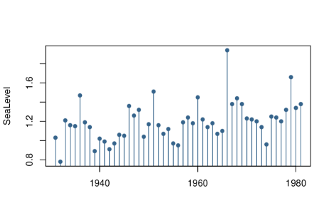
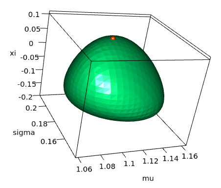
For illustration we will use annual maxima $y_{i}$ for the sea level in Venice Coles (2001). The maxima (in metres) are extracted from the venice data shipped with the R package ismev and rescaled. The simple model $y_{i}\sim_{\text{i.i.d.}}\text{GEV}(\mu,\,\sigma,\,\xi)$ will be used for illustration under the name Venice example. The $95\%$ interval on the shape parameter $\xi$ as found by constrained optimisation is $[-0.197,\,0.098]$. The right part of Figure 2 shows the boundary $\partial\mathcal{R}$ of the region $\mathcal{R}(\delta)$ of (6) in the three-dimensional parameter $\mu\sigma\xi$-space with $\delta:=q_{\chi^{2}(1)}(1-\alpha)/2$. Also shown is the point $\boldsymbol{\theta}$ for which $\xi$ is maximal, corresponding to the upper confidence limit. All 3D plots shown in this article were created by using the R package rgl (Murdoch and Adler 2022).

Figure 2: Venice example. Left: The observations. Right: The contour $\partial\mathcal{R}$ in the parameter space with coordinates $\mu$, $\sigma$ and $\xi$; The little ball in orange on top of the contour surface shows the parameter $\boldsymbol{\theta}$ for which the shape $\xi$ is maximal. The corresponding coordinate $\xi$ is the upper bound $\xi_{\texttt{U}}$ of the confidence interval for $\xi$.

Inferring on a return level

For a given real number $T>1$ called the return period, we will consider the corresponding return level as denoted by $\eta(T;\,\boldsymbol{\theta})$ or simply $\eta(T)$, and defined by

$$\eta(T)=\mu+\sigma\,\eta_{0}(T),\qquad\text{with }\eta_{0}(T):=\begin{cases}\{T^{\xi}-1\}/\xi&\xi\neq 0,\\ \log T&\xi=0.\end{cases}$$ (9)

This is the level which is on average exceeded once in a period with duration $T$ years.

Remark 3.

This definition of the return level is derived from a continuous-time framework rather than from a framework of blocks with a specific duration; It departs slightly from the usual definition of the return level as being the quantile $q_{\texttt{GEV}}(p)$ corresponding to the probability $p:=1-1/T$ see Coles (2001). However the two formulas are the same up to the approximation $-\log[-\log p]\approx-\log(1-p)$ which holds for $p$ close to $1$ hence for large $T$.

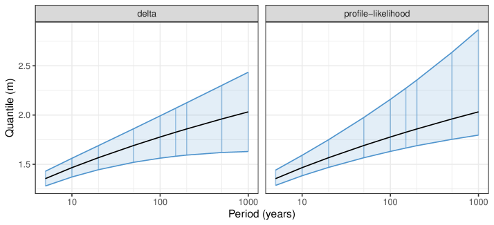
For a given return period $T$, it is straightforward to re-parameterise the model by replacing the location parameter $\mu$ by $\eta(T)$. Both the transformation $[\mu,\,\sigma,\,\xi]^{\top}\mapsto[\eta(T),\,\sigma,\,\xi]^{\top}$ and its reciprocal are easily coped with. However, we usually need to consider several return periods. For example, a popular tool is the so-called return level plot as shown on Figure 3 for the Venice example. The confidence bounds $\eta_{\texttt{L}}(T)$ and $\eta_{\texttt{U}}(T)$ are actually obtained by interpolating the bounds computed at a dozen of return periods $T_{i}$. This was done both for the cheap delta method and for the profile likelihood method using optimisation. Needless to say, the two inference methods produce quite different results.

Remark 4.

For models specifying independent GEV observations, the gradient and Hessian of the log-likelihood $\ell(\boldsymbol{\theta})$ can be obtained in closed form. However, much care must be taken for $\xi\approx 0$ because the exact derivatives are then quite difficult to evaluate, especially at the second order. The gradient of the objective can usually be obtained in closed form, as is obviously the case when the objective is one of the parameters. For the inference on the GEV return period, the gradient of the quantile is difficult to evaluate for $\xi\approx 0$. We used here Taylor approximations as implemented in the R package nieve (Deville 2022).

Figure 3: Return level plot for the Venice example using the cheap delta method (left) and profile likelihood (right). The $95\%$ confidence bounds $\eta_{\texttt{L}}(T)$ and $\eta_{\texttt{U}}(T)$ are computed for the return periods $T_{i}$ shown by a vertical segment. The curve in black shows the return level $\eta(T)$ corresponding to the ML estimate $\hat{\boldsymbol{\theta}}$.

Extreme Value Regression

The GEV distribution is often used in the so-called EV regression framework where a response $y$ is related to a vector of covariates $\mathbf{x}$

$$y\,|\,\mathbf{x}\sim\text{GEV}\{\mu(\mathbf{x}),\,\sigma(\mathbf{x}),\,\xi(\mathbf{x})\},$$

where the functions $\mu(\mathbf{x})$, $\sigma(\mathbf{x})$ and $\xi(\mathbf{x})$ can be specified in parametric form. As a fairly simple example to investigate climate change from block maxima considered as being independent, a scalar time $x$ can be used as covariate for the location parameter as in

$$\mu(x)=\theta_{0}^{\mu}+\theta_{1}^{\mu}x$$ (10)

so the vector $\boldsymbol{\theta}$ of model parameters involves a sub-vector $\boldsymbol{\theta}^{\mu}=[\theta_{0}^{\mu},\,\theta_{1}^{\mu}]^{\top}$ devoted to the GEV location. A similar formula could be used to link the scale $\sigma$ (or its log) or the shape $\xi$ to the covariates. Note that some model parameters could be shared across the three GEV parameters. Anyway, it may be of importance to infer on the trend coefficient $\theta_{1}^{\mu}$.

Using the R package NSGEV Deville and IRSN (2023) a GEV model (10) was fitted for the Venice example data with $x$ being the time, along with a constant scale $\sigma$ and a constant scale $\xi$. The estimate of the trend coefficient $\theta_{1}^{\mu}$ in metres per 100-year was $\widehat{\theta}_{1}^{\mu}=0.565$ and the $95\%$ profile likelihood confidence interval on $\theta_{1}^{\mu}$ was found to be $[0.284,\,0.846]$ by using the constrained optimisation method. However the scaling of $x$ mattered: using the year time unit instead of the 100-year unit led to incorrect confidence limits. These results were checked by using the R package extRemes Gilleland and Katz (2016) which also required some manual tuning in order to get the profile likelihood limits.

In relation with an EV regression one may want to infer on the $T$-year return period $\eta(T,\,\mathbf{x})$ which now depends on $\mathbf{x}$ considered as fixed. In the simple case (10) the parameter $\theta_{0}^{\mu}$ could be replaced by $\eta(T,\,x)$ in a re-parameterisation, provided that $\theta_{0}^{\mu}$ is not involved in the formula for the GEV scale $\sigma$ nor in that for the shape $\xi$. However in a general framework, a re-parameterisation is awkward since the same parameter can be involved in several GEV formulas, possibly in a non-linear fashion. By contrast the optimisation can be implemented for a fairly general framework.

3.5 Practical considerations on computing

Optimisation

For a straightforward application of the optimisation formulation, we can use a routine for constrained optimisation with a general (smooth) constraint. For instance, the NLopt library (Johnson 2022) offers a number of algorithms devoted to such optimisation problems, some of them using the derivatives of the objective and the constraint. This library can be used from several programming languages including R, Python and Julia. The availability of both these exact derivatives in closed form turns out to be a desirable thing for the sake of computing time. In the general case where covariates are used, chain rule must be used to compute the gradient of the log-likelihood. For instance in the EV regression framework above, given $\mathbf{x}_{i}$ and $y_{i}$, the vector $\boldsymbol{\mu}$ of GEV locations $\mu_{i}=\mu(\mathbf{x}_{i})$ is related to the parameter by a linear relation $\boldsymbol{\mu}=\mathbf{X}^{\mu}\boldsymbol{\theta}$, so the differentiation is straightforward. The linearity is not essential here: a non-linear but differentiable link would be used in the same way.

Although most of the available constrained optimisation routines are local, we should ideally use here a global constrained optimisation. The related global algorithms use a local algorithm, hence require some tuning at both the global and the local levels (Johnson 2022).

In order to find suitable initial values, simple algorithms can be designed on the basis of the geometrical interpretation. We can find a vector $\boldsymbol{\theta}$ satisfying the equality $\ell(\boldsymbol{\theta})=\ell_{\max}-\delta$ by using some kind of dichotomy using both points inside and outside of the likelihood contour $\partial\mathcal{R}$. The ML estimate $\hat{\boldsymbol{\theta}}$ can be considered as known, and we can easily find a point outside $\partial\mathcal{R}$ with a line search. Provided that such an algorithm is available in a reliable implementation we can use an equality constraint rather than an inequality constraint for the optimisation.

Our experience is that even apparently simple situations may be surprisingly difficult to cope with. Convergence may be difficult to reach with $p$ as small as $3$ and with a linear function such as $\eta(\boldsymbol{\theta})=\theta_{1}$. Another practical difficulty is to make sure that the convergence was really achieved, which seems more difficult for a constrained optimisation than for an unconstrained one. In the second case, the stopping rule will involve both the change in the objective and that in the constraint, either in absolute or relative variation. Tuning these parameters can be tedious. In the classical zero-finding approach for profile likelihood, a graphical control is most often required since the optimisation used to evaluate the profile log-likelihood may have failed and/or the zero-finding may also have failed. Graphical diagnostics such as a plot of the profile likelihood against the parameter of interest are widely used. These diagnostics also help for the constrained optimisation method, yet if the profile likelihood function is to be repeatedly evaluated, the the constrained optimisation has little benefit.

Using MCMC iterates

Programs devoted to MCMC sampling, a.k.a. MCMC samplers such as JAGS (Plummer 2003) and Stan (Stan Development Team 2022) are widely available and are fast enough for most purposes. Over the last decade, considerable improvements in MCMC sampling have been allowed by the use of Hamiltonian Monte-Carlo and of automatic differentiation as both implemented in Stan. Also, some software dedicated to a specific form of models embed specialised MCMC samplers which can be very fast and over-perform the generalist samplers.

Although this may not be the simplest and fastest way, profile likelihood inference can readily and reliably be obtained by using MCMC iterates. Suppose indeed that on the basis of a prior for $\boldsymbol{\theta}$, a large number $K$ of MCMC iterates $\boldsymbol{\theta}^{[k]}$ have been computed, along with the (unnormalised) log-posterior density $\log p(\boldsymbol{\theta}^{[k)}|\,\mathbf{y})$ and the log-likelihood $\ell(\boldsymbol{\theta}^{[k]})$. In practice, several thousands of iterates are typically made available. These iterates should provide a good coverage of the region with high posterior probability in the parameter space, and it is a common practice to consider the Maximum A posteriori Probability (MAP) estimate as simply being the MCMC iterate for which $\log p(\boldsymbol{\theta}^{[k]}|\,\mathbf{y})$ is maximal. Inasmuch a reasonably non-informative prior for $\boldsymbol{\theta}$ is used, the iterates should cover as well the region with high likelihood and the ML estimate $\hat{\boldsymbol{\theta}}$ can similarly be obtained as the iterate $\boldsymbol{\theta}^{[k]}$ for which $\ell(\boldsymbol{\theta}^{[k]})$ is maximal.

As recalled before, the Bayesian inference on a function $\eta(\boldsymbol{\theta})$ of the parameter, be it scalar-valued or vector-valued, is straightforward. If $\eta(\boldsymbol{\theta})$ is scalar-valued, we get an approximation of the profile likelihood bound $\eta_{\texttt{U}}$ as the maximal value $\eta(\boldsymbol{\theta}^{[k]})$ among the iterates $\boldsymbol{\theta}^{[k]}$ such that the log-likelihood inequality $\ell(\boldsymbol{\theta}^{[k]})\geqslant\ell_{\max}-\delta$ holds. 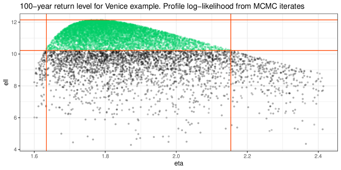Although not required, the profile log-likelihood function $\ell_{\texttt{prof}}(\eta)$ can also in this framework be estimated as the maximum of the log-likelihoods $\ell(\boldsymbol{\theta}^{[k]})$ over the iterates such that $\eta(\boldsymbol{\theta}^{[k]})$ is close to $\eta$. This is illustrated with the Venice example on Figure 4 for the $100$-year return level $\eta(100)$. The MCMC iterates were obtained by using the very efficient rpost_rcpp function of the revdbayes R package (Northrop 2022); The "flatflat" GEV prior was used. For EV regression models with covariates the Stan sampler can be used.

Figure 4: Profile likelihood interval from $K=10^{4}$ MCMC iterates. The $95\%$ limits are for the $100$-year return level $\eta(T)$ for the GEV example. The confidence limits (vertical lines) are the smallest and the largest $\eta(T)$ corresponding to iterates $\boldsymbol{\theta}^{[k]}$ such that $\ell(\boldsymbol{\theta}^{[k]})\geqslant\ell_{\max}-\delta$. The corresponding iterates are shown as green points $[\eta,\,\ell]$. The confidence limits are identical to those obtained by constrained optimisation up to two decimal places.

4 Function with an extra variable and ODE

4.1 Problem

In a number of situations we want to infer on a smooth function $\eta(\boldsymbol{\theta},\,t)$ where $t$ is an extra continuous variable assumed to be scalar. An iconic example is provided by the simple linear regression $y=\theta_{0}+\theta_{1}t+\varepsilon$ where $t$ is a single covariate and $\varepsilon$ is a noise term. This example extends to non-linear regression models with a single covariate and Gaussian noise (Bates and Watts 1988). Another common example is when $\eta(\boldsymbol{\theta},\,t)$ is a probability function such as the cumulative distribution or the quantile function, $t$ being then a quantile or a probability. For the GEV return level problem above, we can take $t$ to be the return period $T$, or some strictly monotonous function of $T$. In such a framework, the confidence interval for $\eta$ will typically be required for several values of $t$ in order to form a confidence band as illustrated with the return level plot above on Figure 3. For consistency with the examples, we will consider the notations $\eta(\boldsymbol{\theta},\,t)$ and $\eta(t;\,\boldsymbol{\theta})$ as equivalent. It will also be convenient to refer to $t$ as the time variable.

4.2 From optimisation to ODE

Going back to the optimisation problem discussed above, the objective now depends on $t$, while the constraint does not. The parameter value $\boldsymbol{\theta}_{\texttt{U}}(t)$ corresponding to the upper confidence bound – now depending on $t$ – remains on the same log-likelihood contour $\partial\mathcal{R}$ as before. Provided that the function $\eta(\boldsymbol{\theta},\,t)$ is smooth, the parameter $\boldsymbol{\theta}_{\texttt{U}}(t)$ moves along a smooth path on $\partial\mathcal{R}$. In the general case where an explicit solution of the optimisation problem does not exist, we can solve as many optimisation problems as there are wanted values $t_{i}$ for $t$. Since $\boldsymbol{\theta}_{\texttt{U}}(t)$ smoothly depends on $t$, the solution for a time $t=t_{i}$ can be used as initial value for the next time $t=t_{i+1}$ or $t=t_{i-1}$, provided that the sequence $t_{i}$ is monotonous. This leads to some savings in the number of iterations, especially if the $t_{i}$ are close to each other. A natural idea to avoid solving many optimisation problems is to find an ODE describing the evolution of $\boldsymbol{\theta}_{\texttt{U}}(t)$. Roughly speaking, the ODE comes by differentiating the KKT conditions with respect to the time $t$ as we now explain.

We will use the dot notation for the derivative w.r.t. the time $t$, as in $\dot{\boldsymbol{\theta}_{\texttt{U}}}(t)$ for the derivative of $\boldsymbol{\theta}_{\texttt{U}}(t)$ and also use $\eta_{\texttt{U}}(t):=\eta\{\boldsymbol{\theta}_{\texttt{U}}(t),\,t\}$. Similarly, $\nu_{\texttt{U}}(t)$ will be the Lagrange multiplier used to find $\boldsymbol{\theta}_{\texttt{U}}(t)$ from the KKT conditions (8a) and (8b) with $\eta(\boldsymbol{\theta})$ replaced by $\eta(\boldsymbol{\theta},\,t)$ in (8a). Since $\boldsymbol{\theta}_{\texttt{U}}(t)$ moves on the boundary $\partial\mathcal{R}$, the derivative vector $\dot{\boldsymbol{\theta}_{\texttt{U}}}(t)$ remains orthogonal to the hyperplane tangent to $\mathcal{R}$ at $\boldsymbol{\theta}_{\texttt{U}}(t)$. This can be stated by differentiating the equation (8b) w.r.t. $t$, which gives

$$\frac{\partial\ell}{\partial\boldsymbol{\theta}^{\top}}\,\dot{\boldsymbol{\theta}_{\texttt{U}}}=0,$$ (11)

where the partial derivative is evaluated at $\boldsymbol{\theta}_{\texttt{U}}(t)$. We can similarly differentiate w.r.t. $t$ the equation (8a) where $\boldsymbol{\theta}$ and $\nu$ are replaced by the solutions $\boldsymbol{\theta}_{\texttt{U}}(t)$ and $\nu_{\texttt{U}}(t)$, leading to

$$\frac{\partial^{2}\eta}{\partial t\partial\boldsymbol{\theta}}+\frac{\partial^{2}\eta}{\partial\boldsymbol{\theta}\partial\boldsymbol{\theta}^{\top}}\,\dot{\boldsymbol{\theta}_{\texttt{U}}}=\dot{\nu_{\texttt{U}}}\,\frac{\partial\ell}{\partial\boldsymbol{\theta}}+\nu_{\texttt{U}}\frac{\partial^{2}\ell}{\partial\boldsymbol{\theta}\partial\boldsymbol{\theta}^{\top}}\,\dot{\boldsymbol{\theta}_{\texttt{U}}},$$ (12)

and by rearranging, (11) and (12) can be written as

$$\begin{bmatrix}-\partial^{2}_{\boldsymbol{\theta},\boldsymbol{\theta}^{\top}}\eta+\nu_{\texttt{U}}\,\{\partial^{2}_{\boldsymbol{\theta},\boldsymbol{\theta}^{\top}}\ell\}&\partial_{\boldsymbol{\theta}}\ell\\ \partial_{\boldsymbol{\theta}^{\top}}\ell&0\rule{0.0pt}{11.99998pt}\end{bmatrix}\begin{bmatrix}\dot{\boldsymbol{\theta}_{\texttt{U}}}\\ \dot{\nu_{\texttt{U}}}\rule{0.0pt}{11.99998pt}\end{bmatrix}=\begin{bmatrix}\partial^{2}_{t,\boldsymbol{\theta}}\eta\\ \rule{0.0pt}{11.99998pt}0\end{bmatrix}.$$ (13)

Provided that the $(p+1)\times(p+1)$ matrix of the left-hand side is invertible, we get an ODE for the vector $\boldsymbol{\theta}_{\texttt{U}}^{\dagger}:=[\boldsymbol{\theta}_{\texttt{U}}^{\top},\,\nu_{\texttt{U}}]^{\top}$. As will be illustrated later, in some cases $\nu_{\texttt{U}}$ can be expressed as a function of $\boldsymbol{\theta}_{\texttt{U}}$ and we then get an ODE

$$\dot{\boldsymbol{\theta}}=\mathbf{b}_{\texttt{U}}(\boldsymbol{\theta},\,t)$$ (14)

where $\mathbf{b}_{\texttt{U}}$ stands for a vector-valued function with arguments $\boldsymbol{\theta}$ and $t$. Anyway, using the ODE requires the availability of the two Hessians for the objective $\eta$ and for the log-likelihood, and also the availability of the $p$ cross derivatives $\partial^{2}_{t,\theta_{k}}\eta$.

Remark 5.

When $\eta(\boldsymbol{\theta},\,t)$ is the value of a cumulative distribution function $F(t;\,\boldsymbol{\theta})$, the cross derivatives $\partial^{2}_{t,\theta_{k}}\eta$ are simply the first-order derivatives $\partial_{\theta_{k}}f$ of the density function $f$, which can be computed from the gradient of the log-likelihood.

Remark 6.

Note that with partial derivatives evaluated at $\boldsymbol{\theta}_{\texttt{U}}(t)$ and $t$, we have

$$\dot{\eta_{\texttt{U}}}=\frac{\partial\eta}{\partial t}+\frac{\partial\eta}{\partial\boldsymbol{\theta}^{\top}}\dot{\boldsymbol{\theta}_{\texttt{U}}}=\frac{\partial\eta}{\partial t}+\nu_{\texttt{U}}^{-1}\frac{\partial\ell}{\partial\boldsymbol{\theta}^{\top}}\dot{\boldsymbol{\theta}_{\texttt{U}}}=\frac{\partial\eta}{\partial t},$$

because $\dot{\boldsymbol{\theta}_{\texttt{U}}}$ is in the hyperplane tangent to $\partial\mathcal{R}$ hence (11 holds. A similar relation holds for the lower bound $\eta_{\texttt{L}}(t)$. This proves that if $\eta(\boldsymbol{\theta},\,t)$ is increasing w.r.t. $t$ for any admissible $\boldsymbol{\theta}$, then both bounds $\eta_{\texttt{L}}$ and $\eta_{\texttt{U}}$ will be increasing w.r.t. $t$, which seems a natural and appealing feature. By contrast, the lower bound given by the delta method may fail to be increasing.

4.3 GEV return levels

We now give some details on the ODE derivation for the inference on the return level $\eta(\boldsymbol{\theta},\,t)$ corresponding to the return period $t$ and related to the GEV distribution with parameter $\boldsymbol{\theta}=[\mu,\,\sigma,\,\xi]^{\top}$. The return level was defined by (9) and the problem was discussed in section 3.4. Because $\partial_{\mu}\eta=1$, we can use the first coordinate of the vector-valued equation $\partial_{\boldsymbol{\theta}}\eta=\nu\,\partial_{\boldsymbol{\theta}}\ell$ to eliminate the Lagrange multiplier $\nu$ from the equations for the two remaining coordinates, getting

$$\left\{\begin{array}[]{r c l}\partial_{\sigma}\eta&=&\partial_{\sigma}\ell\,\left\{\partial_{\mu}\ell\right\}^{-1}\\ \partial_{\xi}\eta&=&\partial_{\xi}\ell\,\left\{\partial_{\mu}\ell\right\}^{-1}.\rule{0.0pt}{11.99998pt}\end{array}\right.$$ (15)

Let $r_{\sigma}$ and $r_{\xi}$ be the two functions of $\boldsymbol{\theta}$ defined by the right-hand sides of the two last equations.

Let $\boldsymbol{\theta}(t)$ be such that the KKT conditions (8a) and (8b) hold for any $t$. Then (15) also holds for any $t$. Note that $r_{\sigma}\{\boldsymbol{\theta}(t)\}$ and $r_{\xi}\{\boldsymbol{\theta}(t)\}$ only depend on $t$ through $\boldsymbol{\theta}(t)$. By differentiating w.r.t. $t$ we get the following next two equations

$$\left\{\begin{array}[]{r c r c r c r}\left[\partial^{2}_{\mu,\sigma}\eta-\partial_{\mu}r_{\sigma}\right]\dot{\mu}&+&\left[\partial^{2}_{\sigma,\sigma}\eta-\partial_{\sigma}r_{\sigma}\right]\dot{\sigma}&+&\left[\partial^{2}_{\xi,\sigma}\eta-\partial_{\xi}r_{\sigma}\right]\dot{\xi}&=&-\partial^{2}_{t,\sigma}\eta,\\ \left[\partial^{2}_{\mu,\xi}\eta-\partial_{\mu}r_{\xi}\right]\dot{\mu}&+&\left[\partial^{2}_{\sigma,\xi}\eta-\partial_{\sigma}r_{\xi}\right]\dot{\sigma}&+&\left[\partial^{2}_{\xi,\xi}\eta-\partial_{\xi}r_{\xi}\right]\dot{\xi}&=&-\partial^{2}_{t,\xi}\eta,\\ \partial_{\mu}\ell\>\dot{\mu}&+&\partial_{\sigma}\ell\>\dot{\sigma}&+&\partial_{\xi}\ell\>\dot{\xi}&=&0.\end{array}\right.$$ (16)

The third equation is a simple translation of the vector form (11). By solving the linear system (16) with unknown $\dot{\boldsymbol{\theta}}$, we get the form (14) above.

The ODE formulation provides nice hints about the confidence bounds.

• When the return period $t$ tends to $\infty$, we may conjecture that the value of $\boldsymbol{\theta}_{\texttt{U}}(t)$ tends to the GEV parameter $\boldsymbol{\theta}$ that maximises the shape parameter $\xi$ for $\boldsymbol{\theta}\in\mathcal{R}$, or equivalently for $\boldsymbol{\theta}\in\partial\mathcal{R}$. This is due to the fact that for large $t$ the return level depends on $\xi$ more heavily than on $\mu$ and $\sigma$.

• It is easily checked that $\partial_{t}\eta(\boldsymbol{\theta},\,t)\geqslant 0$ for any admissible GEV parameter $\boldsymbol{\theta}$. So both the upper and the lower bounds of the confidence interval are increasing with $t$, see Remark 6 above.

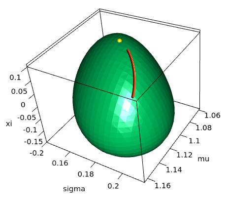
The ODE method is illustrated for the Venice example on Figure 5. The left part shows the upper confidence limit $\eta_{\texttt{U}}(T)$ for several return periods $T$. The right part shows the corresponding path $\boldsymbol{\theta}_{\texttt{U}}(T)$ on the likelihood contour $\partial\mathcal{R}$. The function lsoda from the R package deSolve (Soetaert et al. 2010) was used to compute the numerical solution of the ODE using $1000$ discrete times corresponding to unevenly spaced return periods. The initial value $\boldsymbol{\theta}_{\texttt{U}}(0)$ for $t=0$ was obtained by constrained optimisation.

Figure 5: Confidence interval for the return levels $\eta(t)$ of the Venice example via ODE. Left: The upper bounds $\eta_{\texttt{U}}(t)$ computed by solving the ODE (orange bullets) and those obtained by constrained optimisation (blue squares). Right: The parameters $\boldsymbol{\theta}_{\texttt{U}}(t)$ shown as orange spheres on the surface $\partial\mathcal{R}$ in the parameter $\mu\sigma\xi$-space. The yellow sphere on the very top of the surface shows the value $\boldsymbol{\theta}$ that maximises $\xi$, the corresponding coordinate $\xi$ being the upper bound $\xi_{\texttt{U}}$ of the confidence interval on $\xi$.

5 ODEs and contours

5.1 Profile contours

We now consider the case where the parameter of interest is no longer scalar but is a vector $\boldsymbol{\psi}$ with length $d$, and as before $\boldsymbol{\theta}=[\boldsymbol{\psi}^{\top},\,\boldsymbol{\lambda}^{\top}]^{\top}$. A $d$-dimensional approximate confidence region with level $1-\alpha$ for $\boldsymbol{\psi}$ is defined by

$$\ell_{\texttt{prof}}(\boldsymbol{\psi})\leqslant\ell_{\max}-\delta,\qquad\delta=q_{\chi^{2}(d)}(1-\alpha)/2.$$ (17)

Corresponding to the case where the inequality is an equality, the boundary of the region in the $\boldsymbol{\psi}$-space defined by (17) may be called a profile likelihood contour, or simply: a profile contour. Of special interest is the case $d=2$: the profile contour will generally be a smooth Jordan curve, the interior being the confidence region. We will not try to give conditions ensuring that this kind of favourable situation holds.

The profile contour can be explored by using constrained optimisations. In order to get points $\boldsymbol{\psi}$ on the contour we can indeed optimise some well-chosen scalar functions of the parameter $\boldsymbol{\theta}$ constrained to lie in the $p$-dimensional region $\mathcal{R}(\delta)$ of (6), with the value of $\delta$ related to the length $d$ of the parameter of interest according to (17). For a given vector $\mathbf{a}$ with length $d$, it is intuitively clear that by maximising or minimising $\eta(\boldsymbol{\theta}):=\mathbf{a}^{\top}\boldsymbol{\psi}$ for $\boldsymbol{\theta}$ in $\mathcal{R}(\delta)$, we get a point $\boldsymbol{\theta}^{\star}$ such that $\boldsymbol{\psi}^{\star}:=\boldsymbol{\psi}(\boldsymbol{\theta}^{\star})$ lies on the contour. Moreover, the hyperplane tangent to the contour at $\boldsymbol{\psi}^{\star}$ is orthogonal to $\mathbf{a}$.

As a further step, we can consider a fixed family of vectors $\mathbf{a}(t)$ smoothly depending on a real quantity $t$, say $0\leqslant t\leqslant t^{\star}$, in order to get a continuum of points $\boldsymbol{\psi}^{\star}(t)$ on the contour. We will further assume that $\mathbf{a}(t)$ has an unit Euclidean norm $\|\mathbf{a}(t)\|=1$ for all $t$. The first-order condition is

$$\begin{bmatrix}\mathbf{a}(t)\\ \mathbf{0}\end{bmatrix}=\nu\,\frac{\partial\ell}{\partial\boldsymbol{\theta}},$$ (18)

where $\nu$ is a Lagrange multiplier depending on $t$ and the vector of zeros $\mathbf{0}$ has length $p-d$. Since $\mathbf{a}(t)$ has unit norm, we find $\nu=\pm u(t)^{-1/2}$, where $u(t)$ is defined as the squared norm of the score vector $\partial_{\boldsymbol{\theta}}\ell$ evaluated at $\boldsymbol{\theta}(t)$. We will now on consider only the “plus sign” case $\nu=u(t)^{-1/2}$. It will help to use notations for the score vector and the negative Hessian

$$\mathbf{z}:=\frac{\partial\ell}{\partial\boldsymbol{\theta}},\quad\mathbf{H}:=-\frac{\partial^{2}\ell}{\partial\boldsymbol{\theta}\partial\boldsymbol{\theta}^{\top}},$$ (19)

reminding that these quantities depend on $t$ through $\boldsymbol{\theta}(t)$. We have

$$u(t)=\mathbf{z}^{\top}\mathbf{z}\quad\text{and}\quad\dot{u}(t)=-\dot{\boldsymbol{\theta}}^{\top}\mathbf{H}\,\mathbf{z}-\mathbf{z}^{\top}\,\mathbf{H}\,\dot{\boldsymbol{\theta}}.$$ (20)

By differentiating the first-order condition (18) w.r.t. $t$ we get

$$\begin{bmatrix}\dot{\mathbf{a}}(t)\\ \mathbf{0}\end{bmatrix}=\dot{\nu}\,\frac{\partial\ell}{\partial\boldsymbol{\theta}}+\nu\frac{\partial^{2}\ell}{\partial\boldsymbol{\theta}\partial\boldsymbol{\theta}^{\top}}\,\dot{\boldsymbol{\theta}},$$

where the partial derivatives are in both cases evaluated at $\boldsymbol{\theta}(t)$. Using the fact that $\dot{\nu}=-2^{-1}\dot{u}\,u^{-3/2}$ where $u$ and $\dot{u}$ are given by (20), we get after rearranging

$$\begin{bmatrix}\dot{\mathbf{a}}\\ \mathbf{0}\end{bmatrix}=-u^{-1/2}\,\left\{\mathbf{I}_{p}-\frac{\mathbf{z}\mathbf{z}^{\top}}{\mathbf{z}^{\top}\kern-1.99997pt\mathbf{z}}\right\}\mathbf{H}\,\dot{\boldsymbol{\theta}}=\mathbf{B}\,\dot{\boldsymbol{\theta}}.$$ (21)

In this expression, the matrix between the curly brackets is clearly that of the projection on the orthogonal supplement $\mathbf{z}^{\perp}$ of the linear subspace spanned by $\mathbf{z}$ in $\mathbb{R}^{p}$. So $\mathbf{B}$ has rank $p-1$ and therefore we can not find $\dot{\boldsymbol{\theta}}$ from the sole equation (21). However we have one more equation for $\dot{\boldsymbol{\theta}}$, namely $\mathbf{z}^{\top}\dot{\boldsymbol{\theta}}=0$ and we can get $\dot{\boldsymbol{\theta}}$ as a least squares solution e.g., by using a Housholder QR decomposition of the matrix obtained by adding the new row $\mathbf{z}^{\top}$ to $\mathbf{B}$. Note that the left-hand side of (21) must be orthogonal to $\mathbf{z}$ and the solution of the linear system of $p+1$ equations is then exact, so the equation defines an ODE for $\boldsymbol{\theta}(t)$.

By numerically solving the ODE (21) above, we will find a continuum of points on the contour. As before, we need an initial value $\boldsymbol{\theta}(0)$ which can be obtained by optimisation or by some alternative method as the one described in the next section. In the first case, to account for a possible failure of the constrained optimisation, a few optimisations may be needed to get the initial value. Solving then the ODE is then very fast.

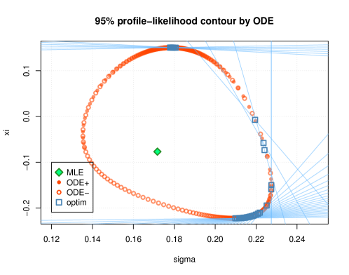
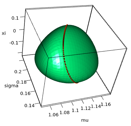
The use of (21) is illustrated on Figure 6 for the Venice example and for the couple of interest $\boldsymbol{\psi}:=[\sigma,\,\xi]^{\top}$. The left panel shows points on the contour obtained by constrained optimisation and by ODE. For the optimisation, a large number of directions $\mathbf{a}$ were tested; When the optimisation succeeded the corresponding point is shown as a square, along with the tangent which by construction must have the prescribed direction. Note that although each square corresponds to an optimisation reported as successful, some problems can still be seen on the right part of the contour: one point is slightly out of the contour and another one does not have the prescribed tangent. For the ODE, we used again the R package deSolve and the vectors $\mathbf{a}(t):=[\cos(t),\,\sin(t)]^{\top}$ with discrete times evenly spaced between $0$ and $2\pi$. The result of a successful optimisation was used as the initial value $\boldsymbol{\theta}(0)$. There are actually two ODE solutions, corresponding to the choice of sign in $\nu=\pm u^{-1/2}$. Both ODE solutions are required to cover the whole contour and the solution paths partially overlap, yet very consistently. The two paths $\boldsymbol{\theta}(t)$ on $\partial\mathcal{R}(\delta)$ are shown in the right panel of Figure 6. An observer located in the parameter space far away in the direction of the $\mu$-axis would see the paths as shown in left panel, the $\sigma$ and the $\xi$ axes then becoming the $x$ and $y$ axes in the usual meaning.

Figure 6: Profile likelihood contour for the GEV parameters $\sigma$ and $\xi$ for the Venice example. Left: Profile contour. Right: the path $\boldsymbol{\theta}(t)$ corresponding to the solution of the ODE. The vector $\boldsymbol{\theta}(t)$ moves on the boundary of the high-likelihood region $\mathcal{R}(\delta)$. Remind that the value of $\delta$ used here corresponds to $d=2$ d.f. hence differs from the one used for the confidence intervals in Figure 2, corresponding to one d.f..

5.2 Log-likelihood contours and confidence level

Turning back to the inference on a smooth scalar function $\eta(\boldsymbol{\theta})$ of the parameter, the ML estimate $\hat{\boldsymbol{\theta}}$ can be used to derive an initial value for a constrained optimisation algorithm. Yet a possibly better use of $\hat{\boldsymbol{\theta}}$ can be made. In the likelihood contour $\partial\mathcal{R}(\delta)$, the quantity $\delta\geqslant 0$ giving the (approximate) confidence level can be regarded as a continuous variable for the optimisation constraint. The variation of $\delta$ should induce a smooth deformation of the likelihood contour $\partial\mathcal{R}(\delta)$. For $\delta\approx 0$ the likelihood region is a small ellipsoid with centre $\hat{\boldsymbol{\theta}}$, and by increasing $\delta$ we get some kind of “inflating bubble”. If we consider both the upper confidence limit $\eta_{\texttt{U}}$ and the related parameter vector $\boldsymbol{\theta}_{\texttt{U}}$ as depending on $\delta$, we can derive an ODE for $\boldsymbol{\theta}_{\texttt{U}}^{\dagger}:=[\boldsymbol{\theta}_{\texttt{U}}^{\top},\,\nu_{\texttt{U}}]^{\top}$ where $\nu_{\texttt{U}}$ is the Lagrange multiplier. Unlike to what occurred before, the vector $\boldsymbol{\theta}_{\texttt{U}}(\delta)$ no longer moves on a given likelihood contour, but instead remains on the surface of the bubble as it goes inflating. The derivation hence slightly differs from what was described above.

Remark 7.

This method is similar to that described by Stapor et al. (2018). However the authors use the log-likelihood as objective and (in our notations) the function $\eta(\boldsymbol{\theta})$ to define an equality constraint as in (3) for the special case $\eta(\boldsymbol{\theta})=\psi$.

To stick to the notations used in the previous sections, we will use the symbol $t$ in place of $\delta$ in the rest of this section. We can derive an ODE for $\boldsymbol{\theta}_{\texttt{U}}^{\dagger}(t)$ by following nearly the same steps as those described in section 4.2. As a major difference, in the constrained optimisation the objective $\eta$ no longer depends on $t$, but the constraint now does. By differentiating (8b) w.r.t. $t$ we now get

$$\frac{\partial\ell}{\partial\boldsymbol{\theta}^{\top}}\,\dot{\boldsymbol{\theta}}_{\texttt{U}}=-1,$$

and the equivalent of (13) for the new framework is now

$$\begin{bmatrix}-\partial^{2}_{\boldsymbol{\theta},\boldsymbol{\theta}^{\top}}\eta+\nu_{\texttt{U}}\,\{\partial^{2}_{\boldsymbol{\theta},\boldsymbol{\theta}^{\top}}\ell\}&\partial_{\boldsymbol{\theta}}\ell\\ \partial_{\boldsymbol{\theta}^{\top}}\ell&0\rule{0.0pt}{11.99998pt}\end{bmatrix}\begin{bmatrix}\dot{\boldsymbol{\theta}_{\texttt{U}}}\\ \dot{\nu_{\texttt{U}}}\rule{0.0pt}{11.99998pt}\end{bmatrix}=\begin{bmatrix}\mathbf{0}\\ \rule{0.0pt}{11.99998pt}-1\end{bmatrix}.$$ (22)

As for the initial condition, we could think of taking $\boldsymbol{\theta}_{\texttt{U}}(0):=\hat{\boldsymbol{\theta}}$. Yet the initial Lagrange multiplier $\nu_{\texttt{U}}(0)$ is now undetermined because the gradient of the log-likelihood $\partial_{\boldsymbol{\theta}}\ell$ is zero at $\hat{\boldsymbol{\theta}}$. However we can instead start from an approximation of the value $\boldsymbol{\theta}_{\texttt{U}}^{\dagger}(\delta_{1})$ corresponding to a small time $\delta_{1}>0$. For a small enough value, the contour of the log-likelihood is approximately an ellipsoid and the function $\eta(\boldsymbol{\theta})$ is approximately linear inside the contour. By reasoning as we did in the linear regression example of Section 3.3, we get the following approximations for $\nu(\delta_{1})$ and $\boldsymbol{\theta}(\delta_{1})$

$$\widetilde{\nu}_{\texttt{U}}(\delta_{1}):=\{\mathbf{h}^{\top}_{0}\mathbf{H}_{0}^{-1}\mathbf{h}_{0}\}^{1/2}/\sqrt{2\delta_{1}},\qquad\widetilde{\boldsymbol{\theta}}_{\texttt{U}}(\delta_{1}):=\hat{\boldsymbol{\theta}}+\widetilde{\nu}_{\texttt{U}}^{-1}(\delta_{1})\,\mathbf{H}^{-1}_{0}\mathbf{h}_{0},$$

where $\mathbf{H}_{0}$ is the Hessian of the negative log-likelihood and $\mathbf{h}_{0}$ is the gradient of $\eta(\boldsymbol{\theta})$, both taken for $\boldsymbol{\theta}=\hat{\boldsymbol{\theta}}$. The matrix $\mathbf{H}_{0}$ should be positive definite. By changing the sign of the initial Lagrange multiplier, the same ODE can be used to find $\boldsymbol{\theta}_{\texttt{L}}(t)$ corresponding to the lower confidence bound.

It may happen that the solution of (22) with the given initial conditions does not exist on the full interval $(0,\,\delta)$ and only exists on a smaller interval, corresponding to a confidence level higher than the one wanted. The region $\mathcal{R}(\delta)$ may indeed fail to be connected, and this can be revealed by the solution of the ODE.

Remark 8.

To a certain extend, solving the ODE (22) is the opposite of maximising the log-likelihood: this somewhat “undoes” what the maximisation did. Considered in reverse time, the ODE admits the equilibrium point $\hat{\boldsymbol{\theta}}$ which is Lyapunov-stable since the log-likelihood is by construction a Lyapunov function.

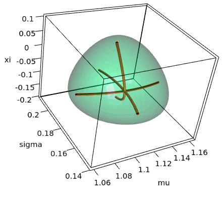
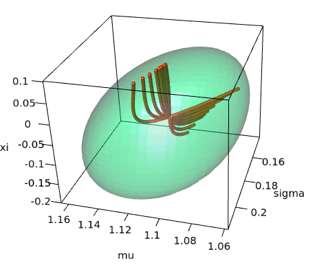
The method is illustrated with the Venice example on Figure 7. The left part shows the paths used to get a confidence interval on each of the three GEV parameters $\mu$, $\sigma$ and $\xi$. For each parameter $\theta_{k}$, two paths are obtained starting from a point close to $\hat{\boldsymbol{\theta}}$ and ending at a point $\boldsymbol{\theta}_{\texttt{L}}^{[k]}$ or $\boldsymbol{\theta}_{\texttt{U}}^{[k]}$ on the contour of the log-likelihood $\partial\mathcal{R}$ such that the parameter of interest $\theta_{k}$ is either minimised or maximised. The right part shows the determination of the upper bound on the return period $\eta(T)$. Nine return periods $T_{i}$ were fixed and for each of them we proceeded as we did for the GEV parameters. In both cases, the paths corresponding to the minimisation and the maximisation of a same quantity are parts of a smooth path that starts from $\boldsymbol{\theta}_{\texttt{L}}$ and ends at the corresponding $\boldsymbol{\theta}_{\texttt{U}}$.

Still using the Venice data, a linear time trend was used in an EV regression as in (10). As was the case with the optimisation method, a suitable scaling was required to get the exact confidence bounds: the unit for the time covariate $x$ had to be set to $100$-year. Interestingly, plotting the Lagrange multiplier $\nu$ against the time of the ODE may provide a valuable diagnostic. The value $\nu(t)$ seems to tend to a limit for large $t$ and when the parameter is not suitably scaled the limit is reached in a few time steps.

Remark 9.

It is easy to see from (22) that when $\eta$ is a linear function of $\boldsymbol{\theta}$ the Lagrange multiplier $\nu(t)$ is a monotonous function of the time. The $2$-nd order derivative of $\eta$ then cancels.

Figure 7: Likelihood contour and paths corresponding to the solution of the ODEs for the Venice example. Left: Six paths corresponding to the determination of lower and upper confidence bounds for the three GEV parameters. Right: Paths corresponding to the lower and upper bounds for nine return periods. In both cases each path starts from a point close to the ML estimate $\hat{\boldsymbol{\theta}}$ and ends at a point on the contour which is shown as the semi-transparent green surface.

The method described here is both very simple and fairly general. It can be used to provide initial values for another ODE computation as introduced in Sections 4.3 and 5.1, a constrained optimisation then no longer being required. For instance, for the GEV return levels we could find a path from $\hat{\boldsymbol{\theta}}$ to the vector $\boldsymbol{\theta}_{\texttt{U}}^{[j]}$ corresponding to the maximisation of $\eta(T_{j})$ for some return period $T_{j}$, and then solve an ODE with a time related to the return period, as discussed in Section 4.3. In other words, we could move from the point $\hat{\boldsymbol{\theta}}$ inside the region $\mathcal{R}(\delta)$ to a point $\boldsymbol{\theta}_{\texttt{U}}^{[j]}$ on the boundary and then move on the boundary, rather than repeatedly move from $\hat{\boldsymbol{\theta}}$ to a boundary point as shown on the right side of Figure 7. The first option should be faster, but using both these two fast approaches provides a basis for checks that can increase the trustworthiness of an implementation.

6 Conclusion and discussion

6.1 Using optimisation and ODEs

The determination of a profile likelihood confidence interval can be formulated as a constrained optimisation problem. Since high quality optimisation routines are widely available, this provides a practical way to compute confidence intervals for the parameters or for a smooth function of the parameter vector. This is especially interesting for models defined via formulas, as a re-parametrisation is then generally difficult to achieve. A practical difficulty is to ensure the convergence of the constrained optimisation, which requires some fine tuning of the algorithm as well as suitable initial values. This motivated the implementation of dedicated optimisation algorithms by Fisher and Lewis (2021) and by Borisov and Metelkin (2020). If MCMC iterates are available corresponding to a reasonably non-informative prior, the constrained optimisation formulation leads to a very simple determination of the profile likelihood intervals, which can be useful when the log-likelihood function is difficult to optimise. Wiping out the effect of the prior is then easily achieved.

In the case where the smooth function depends on an extra continuous “time” variable, an ODE formulation based on the Lagrangian can lead to some interesting theoretical and geometrical findings and provides as well a solution to efficiently compute a batch of confidence intervals, as often required in practice. Only one optimisation is then required, in order to get an initial value. The same technique can be used to compute profile likelihood contours when the interest is on a couple of parameters. Finally, by considering the confidence level as being the time variable, we can derive as well an ODE that exempts from the use of any constrained optimisation routine and provides a very fast determination of the confidence interval(s). ODE solvers are fast and require little tuning, hence may provide a valuable alternative to constrained optimisation routines.

Interestingly, whatever be the parameter of interest, the ODEs used here have their state vector being the parameter vector $\boldsymbol{\theta}$, possibly augmented by a scalar Lagrange multiplier. While MCMC sampling uses a stochastic differential or finite-difference equation to explore the region of high posterior density in the parameter space, we used here ordinary differential equations to explore the region with high likelihood. These ODEs can be said interest-driven inasmuch they put emphasis on the parameter of interest.

These techniques have been illustrated for models implying the GEV distribution, with a small number of parameters. However, they apply to any parametric model. A practical limitation is that the evaluation of the log-likelihood and its derivatives must be fast enough to afford hundreds of evaluations, but this limitation also holds for the inference based on MCMC. Some further experimentation will be required to better assess the practical acceptability and the trustworthiness of the techniques described above. The ODE approach could be compared to other methods or implementations and some porting between the languages R, Python and Julia could benefit to a larger community of users.

6.2 Limitations and possible extensions

A practical limitation met both in the optimisation and the ODE method is the need of scaling the parameters. However at least for EV regression models, simple solutions could be used to avoid a manual scaling. The QR decomposition or the singular value decomposition of the design matrices such as $\mathbf{X}^{\mu}$ both could be used.

As a theoretical limitation, no simple condition exists to grant that a given function of the parameter can indeed be considered as a parameter of the model as was assumed in the derivation. This relates to the question of practical identifiability discussed in Fisher and Lewis (2021) and Borisov and Metelkin (2020). Only sufficient conditions can be derived for some specific forms of models, and especially for EV regressions with linear links as often used in practice. An interesting property of the GEV distribution as above parameterised is that the dependence on each parameter is increasing for the stochastic ordering. For instance by increasing $\mu$ for given $\sigma$ and $\xi$, we get a distribution which is larger in the stochastic ordering. So if by increasing a given parameter $\theta_{k}$ we are certain to increase $\mu$, then we will then also increase the distribution in the stochastic ordering. This may be of some help in the analysis.

The ideas discussed here could be applied when the quantity of interest depends smoothly on several variables $t_{i}$ e.g., takes the form $\eta(t_{1},t_{2};\,\boldsymbol{\theta})$ for two variables $t_{1}$ and $t_{2}$. Each bound of the confidence interval could then be obtained by solving a vector-valued Partial Differential Equation (PDE) rather than an ODE. The PDE can be derived by differentiating the KKT conditions w.r.t. the variables $t_{i}$.

The techniques described above could be used for Bayesian inference by simply replacing the log-likelihood by the log-posterior, provided that the prior is smooth enough and that its first and second order derivatives are available. This may be useful e.g., if a high a posteriori probability contour is to be found within a very small computing time. However, in order to control the posterior probability level, some quadrature will be required.

In order to improve the coverage rate of the intervals in the small sample case, a modified profile likelihood can be used in place of the profile likelihood, see Davison (2003), Barndorff-Nielsen and Cox (1994). The confidence bounds related to the modified profile can no longer be obtained by the constrained optimisation described above, but the question arises whether similar improvements could be reached by replacing the log-likelihood by a suitably modified log-likelihood in the constraint.

Appendix A Proof of proposition 1

We first show that $\psi^{\star}\leqslant\psi_{\texttt{U}}$. By definition of the profile log-likelihood, we have

$$\ell_{\texttt{prof}}(\psi^{\star})=\ell\{\psi^{\star},\,\hat{\boldsymbol{\lambda}}(\psi^{\star})\}\geqslant\ell(\psi^{\star},\,\boldsymbol{\lambda}^{\star})\geqslant\ell_{\max}-\delta,$$

because $\psi^{\star}$ and $\boldsymbol{\lambda}^{\star}$ together form the solution $\boldsymbol{\theta}^{\star}$ of problem (5) which is in the feasible set. Since $\ell_{\max}-\delta=\ell_{\texttt{prof}}(\psi_{\texttt{U}})$ and since the profile log-likelihood is assumed to be decreasing for $\psi\geqslant\hat{\psi}$, we see that $\psi^{\star}$ is located at the left of the upper bound $\psi_{\texttt{U}}$ i.e. $\psi^{\star}\leqslant\psi_{\texttt{U}}$.

To see that $\psi_{\texttt{U}}\leqslant\psi^{\star}$, observe that $\psi_{\texttt{U}}$ takes the form $\psi(\boldsymbol{\theta})$ for some $\boldsymbol{\theta}$ with $\ell(\boldsymbol{\theta})\geqslant\ell_{\max}-\delta$, namely for $\boldsymbol{\theta}$ taken equal to the vector $\boldsymbol{\theta}_{\texttt{U}}$ with components $\psi_{\texttt{U}}$ and $\hat{\boldsymbol{\lambda}}(\psi_{\texttt{U}})$. Indeed, then $\ell(\boldsymbol{\theta}_{\texttt{U}})=\ell_{\texttt{prof}}(\psi_{\texttt{U}})=\ell_{\texttt{max}}-\delta$ by (1). Since $\boldsymbol{\theta}_{\texttt{U}}$ is therefore in the feasible set of problem (5), we have $\psi(\boldsymbol{\theta}_{\texttt{U}})\leqslant\psi^{\star}$ i.e. $\psi_{\texttt{U}}\leqslant\psi^{\star}$ as claimed.

References

- Barndorff-Nielsen and Cox (1994) Barndorff-Nielsen O, Cox D (1994). Inference and Asymptotics. Monographs on Statistics and Applied Probability. Chapman & Hall.
- Bates and Watts (1988) Bates D, Watts D (1988). Nonlinear Regression Analysis & Its Applications. Wiley series in probability and mathematical statistics. Wiley. doi:10.1002/9780470316757.
- Belzile (2023) Belzile LR (2023). mev: Modelling of Extreme Values. URL https://lbelzile.github.io/mev/.
- Borisov and Metelkin (2020) Borisov I, Metelkin E (2020). “Confidence intervals by constrained optimization. An algorithm and software package for practical identifiability analysis in systems biology.” PLoS Computational Biology, 16(20). doi:10.1371/journal.pcbi.1008495.
- Coles (2001) Coles S (2001). An Introduction to Statistical Modelling of Extreme Values. Springer. doi:10.1007/978-1-4471-3675-0.
- Davison (2003) Davison A (2003). Statistical Models. Cambridge Series in Statistical and Probabilistic Mathematics. Cambridge University Press. doi:10.1017/CBO9780511815850.
- Deville (2022) Deville Y (2022). nieve: Miscellaneous Utilities for Extreme Value Analysis. R package version 0.1.1, URL https://github.com/yvesdeville/nieve/.
- Deville and IRSN (2023) Deville Y, IRSN (2023). NSGEV: Non-Stationnary GEV Time Series. URL https://IRSN.github.io/NSGEV/.
- Fisher and Lewis (2021) Fisher SM, Lewis MA (2021). “A Robust and Efficient Algorithm to Find Profile Likelihood Confidence Intervals.” Statistics and Computing, 31(4). doi:10.1007/s11222-021-10012-y.
- Gilleland and Katz (2016) Gilleland E, Katz RW (2016). “extRemes 2.0: An Extreme Value Analysis Package in R.” Journal of Statistical Software, 72(8), 1–39. doi:10.18637/jss.v072.i08.
- Johnson (2022) Johnson SG (2022). The NLopt Nonlinear-Optimization Package. URL https://nlopt.readthedocs.io/en/latest.
- Murdoch and Adler (2022) Murdoch D, Adler D (2022). rgl: 3D Visualization Using OpenGL. R package version 0.108.3.2, URL https://CRAN.R-project.org/package=rgl.
- Northrop (2022) Northrop PJ (2022). revdbayes: Ratio-of-Uniforms Sampling for Bayesian Extreme Value Analysis. R package version 1.4.9, URL https://CRAN.R-project.org/package=revdbayes.
- Plummer (2003) Plummer M (2003). “JAGS: A Program for Analysis of Bayesian Graphical Models Using Gibbs Sampling.” In Proceedings of the 3-rd International Workshop on Distributed Statistical Computing (DSC 2003), Vienna, 20-22 March 2003.
- R Core Team (2022) R Core Team (2022). R: A Language and Environment for Statistical Computing. R Foundation for Statistical Computing, Vienna, Austria. URL https://www.R-project.org/.
- Soetaert et al. (2010) Soetaert K, Petzoldt T, Setzer RW (2010). “Solving Differential Equations in R: Package deSolve.” Journal of Statistical Software, 33(9), 1–25. doi:10.18637/jss.v033.i09.
- Stan Development Team (2022) Stan Development Team (2022). Stan Modeling Language Users Guide and Reference Manual. URL https://mc-stan.org.
- Stapor et al. (2018) Stapor P, Fröhlich F, Hasenauer J (2018). “Optimization and Profile Calculation of ODE Models using Second Order Adjoint Sensitivity Analysis.” Bioinformatics, 34(13), i151–i159. ISSN 1367-4803. doi:10.1093/bioinformatics/bty230. URL https://doi.org/10.1093/bioinformatics/bty230.
- Stephenson (2002) Stephenson AG (2002). “evd: Extreme Value Distributions.” R News, 2(2), 0. URL https://CRAN.R-project.org/doc/Rnews/.
- Stephenson and Heffernan (2018) Stephenson AG, Heffernan JE (2018). ismev: An Introduction to Statistical Modeling of Extreme Values. R package version 1.42, URL https://CRAN.R-project.org/package=ismev.
- Venzon and Moolgavkar (1988) Venzon D, Moolgavkar S (1988). “A Method for Computing Profile-Likelihood-Based Confidence Intervals.” Applied Statistics, 37(1). doi:10.2307/2347496.