Locking-free hybrid high-order method for linear elasticity

Abstract.

The hybrid-high order (HHO) scheme has many successful applications including linear elasticity as the first step towards computational solid mechanics. The striking advantage is the simplicity among other higher-order nonconforming schemes and its geometric flexibility as a polytopal method on the expanse of a parameter-free refined stabilization. The classical suggestion of a locking-free HHO discretization requires a split of the the reconstruction terms with an additional reconstruction of the divergence operator that might be motivated by the Stokes equations for the robust approximation in the incompressible limit, when one Lamé parameter $\lambda\to\infty$ becomes very large. This paper utilizes just one reconstruction operator for the linear Green strain and therefore does not rely on a split in deviatoric and spherical behavior. The a priori error analysis provides quasi-best approximation with $\lambda$-independent equivalence constants. The reliable and (up to data oscillations) efficient a posteriori error estimates are stabilization-free and $\lambda$-robust. The error analysis is carried out on simplicial meshes to allow conforming piecewise polynomials finite elements in the kernel of the stabilization terms. Numerical benchmarks provide empirical evidence for optimal convergence rates of the a posteriori error estimator in some associated adaptive mesh-refining algorithm also in the incompressible limit.

1. Introduction

1.1. Motivation

The first HHO elasticity model has been analyzed in [16] with emphasis on general meshes and two different recovery operators for the linear Green strain and for the divergence of the displacements. The a priori error analysis therein provides $\lambda$-robust convergence rates relative to the possibly restricted elliptic regularity on polygons with general boundary conditions of changing type. The first paper on the HHO in nonlinear elasticity [5] suggests an HHO method with one recovery operator for the linear Green strain tensor, which was analyzed in [18]. Optimal convergence rates are presented in [16, 18] under unrealistic regularity assumptions on the exact solutions so that higher convergence rates of higher-order HHO versions are not visible for quasi-uniform triangulations in typical benchmark problems of computational mechanics.

This paper provides quasi-best approximation results for a discrete problem with a smoother [26, 27, 20, 10] and without (up to data oscillations for $L^{2}$ source terms) that immediately opens the door to superior adaptive mesh-design. The tools in the proofs are some right-inverse as in [20] (and many other nonconforming schemes [26, 27, 10]), a deeper understanding of the HHO stabilization, and $\lambda$-robust regularity estimates. One emphasis is on stabilization-free a  posteriori error estimates that are of current interest in the convergence analysis of adaptive mesh-refining algorithms [28]. While HHO methods can be defined on polytopal meshes, the error analysis of this paper exploits the orthogonality of the stress error with conforming test functions. Therefore, it is restricted to regular triangulations into simplices. The cost is a less flexible mesh design but the analysis does not require a sufficiently large parameter in the stabilization as in [28].

1.2. Mathematical model

Let $\Omega\subset\mathbb{R}^{n}$ with $n=2,3$ be a bounded polyhedral Lipschitz domain in two or three space dimensions with boundary $\partial\Omega$ that is split into a closed Dirichlet part $\Gamma_{\mathrm{D}}\subset\partial\Omega$ of positive surface measure and a remaining Neumann part $\Gamma_{\mathrm{N}}\coloneqq\partial\Omega\setminus\Gamma_{\mathrm{D}}$. Given $f\in L^{2}(\Omega)^{n}$ and $g\in L^{2}(\Gamma_{\mathrm{N}})^{n}$, the model problem in linear elasticity of this paper seeks the solution $u\in H^{1}(\Omega)^{n}$ to

(1.1) $$-\mathrm{div}\,\sigma=f\text{ in }\Omega,\quad\sigma\coloneqq\mathbb{C}\varepsilon(u),\quad u=0\text{ on }\Gamma_{\mathrm{D}},\quad\sigma\nu=g\text{ on }\Gamma_{\mathrm{N}}.$$

The linearized Green strain $\varepsilon(v)\coloneqq\mathrm{sym}(\mathrm{D}v)$ is the symmetric part of the gradient $\mathrm{D}v$ and the isotropic elasticity tensor $\mathbb{C}$ acts as $\mathbb{C}E\coloneqq\lambda\mathrm{tr}(E)\mathrm{I}_{n\times n}+2\mu E$ for any $E\in\mathbb{S}\equiv\mathbb{R}_{\mathrm{sym}}^{n\times n}$ with the Lamé parameters $\lambda\geq 0$ and $\mu>0$. We assume that, for $|\Gamma_{\mathrm{N}}|>0$, the parameters $\lambda$, $\mu$ are piecewise constant such that $\mu$ is bounded away from zero $0<\mu_{0}\leq\mu\leq\mu_{1}$ by positive numbers $\mu_{0}\leq\mu_{1}$ and, for $|\Gamma_{\mathrm{N}}|=0$, $\lambda$ and $\mu$ are positive constants. The weak formulation seeks the solution $u\in V\coloneqq\{v\in H^{1}(\Omega)^{n}:v=0\text{ on }\Gamma_{\mathrm{D}}\}$ to

(1.2) $$\int_{\Omega}\mathbb{C}\varepsilon(u):\varepsilon(v)\,\mathrm{d}x=\int_{\Omega}f\cdot v\,\mathrm{d}x+\int_{\Gamma_{\mathrm{N}}}g\cdot v\,\mathrm{d}s\quad\text{for all }v\in V.$$

1.3. Main results

The HHO methodology [17, 16, 18] allows for a reconstruction operator $\mathcal{G}:V_{h}\to P_{k}(\mathcal{T})^{n\times n}$ of the gradient from a discrete ansatz space $V_{h}$ of $V$ onto the space $P_{k}(\mathcal{T})^{n\times n}$ of matrix-valued piecewise polynomials of degree at most $k$. The approximation $\mathbb{C}\varepsilon_{h}$ of $\mathbb{C}\varepsilon$ with $\varepsilon_{h}\coloneqq\mathrm{sym}\,\mathcal{G}$ does not rely on a split in deviatoric and spherical behavior as in [16]. This was proposed in [5] and the HHO method therein seeks the solution $u_{h}\in V_{h}$ to

$$a_{h}(u_{h},v_{h})=F_{h}(v_{h})\quad\text{for any }v_{h}\in V_{h}$$

with a scalar product $a_{h}$ in $V_{h}$ and bounded linear functional $F_{h}$. The reconstruction operator $\varepsilon_{h}$ leads to a straight-forward definition of the discrete stress $\sigma_{h}\coloneqq\mathbb{C}\varepsilon_{h}u_{h}$ with the $L^{2}$ orthogonality $\sigma-\sigma_{h}\perp\varepsilon(P_{k+1}(\mathcal{T})^{n}\cap V)$. The latter allows for the application of the tr-div-dev lemma in the error analysis for $\lambda$-robust estimates. We establish, up to data oscillations, the quasi-best approximation

$$\|\sigma-\sigma_{h}\| +\|\mathrm{I}u-u_{h}\|_{a_{h}}+|u_{h}|_{\mathrm{s}}$$

(1.3) $$\leq C_{\mathrm{ba}}(\|(1-\Pi_{\mathcal{T}}^{k})\sigma\|+\mathrm{osc}(f,\mathcal{T})+\mathrm{osc}(g,\mathcal{F}_{\mathrm{N}}))$$

under a mild assumption on the geometry, where $\mathrm{I}:V\to V_{h}$ is the canonical interpolation in the HHO methodology, $\|\bullet\|_{a_{h}}$ is the norm induced by $a_{h}$, $|\bullet|$ is the seminorm induced by the stabilization, and $\Pi_{\mathcal{T}}^{k}$ is the $L^{2}$ projection onto piecewise polynomials. Notice that (1.3) holds under minimal regularity assumption on $u$, while [16, 18] requires at least piecewise $H^{s}$ regularity of the stress $\sigma$ for some $s>1/2$, which is not available for boundary conditions of changing type on a straight line. The proof of (1.3) utilizes the arguments of [20, 2] but additionally requires a quasi-best approximation result for the stabilization in the spirit of [14]. In addition to (1.3), we derive $L^{2}$ error estimates with additional convergence rates depending on the elliptic regularity on polyhedral domains. If $f\in H^{-1}(\Omega)^{n}$ and $g\in\widetilde{H}^{-1/2}(\Gamma_{\mathrm{N}})^{n}$ are nonsmooth, a modified HHO solver with a smoother [26, 27, 20, 10] is proposed with the oscillation-free a priori error estimate $\|\sigma-\sigma_{h}\|+\|\mathrm{I}u-u_{h}\|_{a_{h}}+|u_{h}|_{\mathrm{s}}\lesssim\|(1-\Pi_{\mathcal{T}}^{k})\sigma\|$.

A consequence of (1.3) is the efficiency of the stabilization. This allows for a stabilization-free a posteriori error analysis as a generalization to [2]. We establish

(1.4) $$C_{\mathrm{rel}}^{-1}\|\sigma-\sigma_{h}\|\leq\eta\leq C_{\mathrm{eff}}(\|\sigma-\sigma_{h}\|+\mathrm{osc}(f,\mathcal{T})+\mathrm{osc}(g,\mathcal{F}_{\mathrm{N}})).$$

with the error estimator

$$\eta^{2} \coloneqq\|h_{\mathcal{T}}(f+\mathrm{div}_{\mathrm{pw}}\sigma_{h})\|^{2}+\mu^{2}\min_{v\in V}\|\varepsilon(v)-\varepsilon_{h}u_{h}\|^{2}$$

(1.5) $$\qquad+\sum_{F\in\mathcal{F}(\Omega)}h_{F}\|[\sigma_{h}]_{F}\nu_{F}\|_{L^{2}(F)}^{2}+\sum_{F\in\mathcal{F}_{\mathrm{N}}}h_{F}\|g-\sigma_{h}\nu_{F}\|_{L^{2}(F)}^{2}.$$

All the constants $C_{\mathrm{ba}}$, $C_{\mathrm{rel}}$, $C_{\mathrm{eff}}$, and those throughout this paper do not depend on the parameter $\lambda$. In the computations, we chose $v=\mathcal{A}u_{h}$ in (1.3) with the nodal average $\mathcal{A}u_{h}$ of the potential reconstruction $\mathcal{R}u_{h}$ of $u_{h}$. This choice is efficient as shown in Section 4 below.

1.4. Outline

The remaining parts of this paper are organized as follows. Section 2 introduces the discrete problem with the aforementioned reconstruction operators and stabilization. Best approximation and $L^{2}$ error estimates follow in Section 3. Section 4 derives $\lambda$-robust stabilization-free reliable and efficient a posteriori error estimates. Computational benchmarks in Section 5 provide numerical evidence for $\lambda$-robustness.

1.5. General notation

Standard notation for Sobolev and Lebesgue spaces applies throughout this paper. In particular, $(\bullet,\bullet)_{L^{2}(\Omega)}$ denotes the $L^{2}$ scalar product and induces the norm $\|\bullet\|\coloneqq\|\bullet\|_{L^{2}(\Omega)}$ in $L^{2}(\Omega)$ and any product $L^{2}(\Omega)^{n}$ or $L^{2}(\Omega)^{n\times n}$ thereof. The norm $\|\bullet\|_{-1}$ in the dual space $H^{-1}(\Omega)$ of $H^{1}_{0}(\Omega)$ reads

(1.6) $$\|F\|_{-1}\coloneqq\sup\nolimits_{v\in H^{1}_{0}(\Omega)\setminus\{0\}}F(v)/\|\nabla v\|.$$

For any $\Phi,\Psi\in L^{2}(\Omega)^{n\times n}$ and $s\in\mathbb{R}$, abbreviate $(\Phi,\Psi)_{\mathbb{C}^{s}}\coloneqq(\mathbb{C}^{s}\Phi,\Psi)_{L^{2}(\Omega)}$ and $\|\Psi\|_{\mathbb{C}^{s}}^{2}\coloneqq(\Psi,\Psi)_{\mathbb{C}^{s}}$. The symmetric and asymmetric part of the gradient $\mathrm{D}v$ of some function $v$ are denoted by $\varepsilon(v)\coloneqq\mathrm{sym}(\mathrm{D}v)$ and $\mathrm{D}_{\mathrm{ss}}v\coloneqq\mathrm{asym}(\mathrm{D}v)$ with the formula $\mathrm{sym}(M)\coloneqq(M+M^{t})/2$ and $\mathrm{asym}(M)\coloneqq(M-M^{t})/2$ for any $M\in\mathbb{R}^{n\times n}$. The Korn inequality

(1.7) $$\|v\|_{H^{1}(\Omega)}\leq C_{\mathrm{K}}\|\varepsilon(v)\|$$

holds for Sobolev functions $v\in H^{1}(\Omega)^{n}$ subject to different constraints to fix the rigid body motions. For $v\in V$, (1.7) is often referred as the first Korn inequality with a constant $C_{\mathrm{K}}$ that exclusively depends on $\Omega$ and $\Gamma_{\mathrm{D}}$. The second Korn inequality is (1.7) for any $v\in H^{1}(\Omega)^{n}$ with

(1.8) $$\int_{\Omega}v\,\mathrm{d}x=0\quad\text{and}\quad\int_{\Omega}\mathrm{D}_{\mathrm{ss}}v\,\mathrm{d}x=0.$$

A proof of all this is given in [7]. The second Korn inequality is applied to piecewise $H^{1}$ vector fields, where (1.8) holds element-wise. In this case, $C_{\mathrm{K}}$ exclusively depends on the dimension $n$ and the shape regularity of the underlying triangulation. The set of symmetric matrices is denoted by $\mathbb{S}\equiv\mathrm{sym}(\mathbb{R}^{n\times n})$. Given two vectors $a,b\in\mathbb{R}^{n}$, recall the vector product $a\otimes b\coloneqq ab^{t}\in\mathbb{R}^{n\times n}$. The deviatoric part of $M\in\mathbb{R}^{n\times n}$ is defined by $\mathrm{dev}M\coloneqq M-\mathrm{tr}(M)\mathrm{I}_{n\times n}/n$ with the trace $\mathrm{tr}(M)\coloneqq M:\mathrm{I}_{n\times n}$. The notation $A\lesssim B$ means $A\leq CB$ for a generic constant $C$, $A\approx B$ abbreviates $A\lesssim B$ and $B\lesssim A$. The constant $C$ may depend on $\mu_{0}$, $\mu_{1}$ but is independent of the critical parameter $\lambda$ and the mesh-size.

2. Discrete problem

This section recalls the HHO methodology introduced in [17, 16, 18, 15] for the linear elastic model problem of Subsection 1.2.

2.1. Triangulation

Let $\mathcal{T}$ be a regular triangulation into simplices with the set of sides $\mathcal{F}$. The set of interior sides is denoted by $\mathcal{F}(\Omega)$ and $\mathcal{F}(\partial\Omega)\coloneqq\mathcal{F}\setminus\mathcal{F}(\Omega)$ is the set of all boundary sides. We assume that the Dirichlet boundary $\Gamma_{\mathrm{D}}$ can be exactly resolved by the triangulation, i.e., the set of Dirichlet sides $\mathcal{F}_{\mathrm{D}}\coloneqq\{F\in\mathcal{F}:F\subset\Gamma_{\mathrm{D}}\}$ covers $\Gamma_{\mathrm{D}}=\cup\mathcal{F}_{\mathrm{D}}$. Fix the orientation of the normal vector $\nu_{F}$ of an interior side $F\in\mathcal{F}(\Omega)$ and $\nu_{F}\coloneqq\nu|_{F}$ for any boundary side $F\in\mathcal{F}(\partial\Omega)$. Given any interior side $F\in\mathcal{F}(\Omega)$, $T_{+}\in\mathcal{T}$ (resp. $T_{-}\in\mathcal{T}$) denotes the unique simplex with $F\subset\partial T_{+}$ (resp. $F\subset\partial T_{-}$) and $\nu_{T_{+}}|_{F}=\nu_{F}$ (resp. $\nu_{T_{-}}|_{F}=-\nu_{F}$). The jump $[v]_{F}$ of any function $v:\Omega\to\mathbb{R}$ with $v|_{T_{\pm}}\in W^{1,1}(\mathrm{int}(T_{\pm}))$ along $F\in\mathcal{F}(\Omega)$ is defined by $[v]_{F}\coloneqq v|_{T_{+}}-v|_{T_{-}}\in L^{1}(F;\mathbb{R}^{m})$. If $F\in\mathcal{F}(\partial\Omega)$, then $[v]_{F}\coloneqq v|_{F}$. For any $T\in\mathcal{T}$ (resp. $F\in\mathcal{F}$), define the simplex patch $\Omega(T)\coloneqq\mathrm{int}(\cup_{T\in\mathcal{T},T\cap T\neq\emptyset}T)$ (resp. side patch $\omega(F)\coloneqq\mathrm{int}(\cup_{T\in\mathcal{T},F\in\mathcal{F}(T)}T)$). The set $H^{1}(\mathcal{T})$ is the space of all piecewise $H^{1}$ function with respect to the triangulation $\mathcal{T}$. The notation $\nabla_{\mathrm{pw}}$ denotes the piecewise application of the differential operator $\nabla$ (even without explicit reference to $\mathcal{T}$). This notation applies to the differential operators $\mathrm{div}$ and $\varepsilon$ as well. In context of mesh-refining algorithms, there is an initial triangulation $\mathcal{T}_{0}$ with the set $\mathcal{V}_{0}$ (resp. $\mathcal{F}_{0}$) of vertices (resp. sides) of $\mathcal{T}_{0}$. We assume that $\mathcal{T}_{0}$ satisfies the initial condition (IC) from [25, Section 4, (a)–(b)] to guarantee that the triangulations generated by successive refinements of $\mathcal{T}_{0}$ with the newest-vertex-bisection (NVB) algorithm [22, 25] are shape-regular. The set of all such triangulations is denoted by $\mathbb{T}$ and $\mathcal{T}\in\mathbb{T}$ is understood throughout the remaining parts of this paper.

2.2. Finite element spaces

Given a subset $M\subset\mathbb{R}^{n}$ of diameter $h_{M}$, let $P_{k}(M)$ denote the space of polynomials on $M$ of total degree at most $k$. For any $v\in L^{1}(M)$, $\Pi_{M}^{k}v\in P_{k}(M)$ denotes the $L^{2}$ projection of $v$ onto $P_{k}(M)$. The space of piecewise polynomials of degree at most $k$ with respect to the triangulation $\mathcal{T}$ (resp. the sides $\mathcal{F}$) is denoted by $P_{k}(\mathcal{T})$ (resp. $P_{k}(\mathcal{F}))$. The continuous version of $P_{k+1}(\mathcal{T})^{n}$ with vanishing boundary data on $\Gamma_{\mathrm{D}}$ reads $S_{\mathrm{D}}^{k+1}(\mathcal{T})\coloneqq P_{k+1}(\mathcal{T})^{n}\cap V$. Given $v\in L^{1}(\Omega)$, the $L^{2}$ projection $\Pi_{\mathcal{T}}^{k}v$ of $v$ onto $P_{k}(\mathcal{T})$ is $(\Pi_{\mathcal{T}}^{k}v)|_{T}=\Pi_{T}^{k}v|_{T}$ in any simplex $T\in\mathcal{T}$. The triangulation $\mathcal{T}$ gives rise to the piecewise constant mesh-size function $h_{\mathcal{T}}\in P_{0}(\mathcal{T})$ with $h_{\mathcal{T}}|_{T}=h_{T}$; $h_{\max}\coloneqq\max_{T\in\mathcal{T}}h_{T}$ is the maximal mesh-size of $\mathcal{T}$. For any $f\in L^{2}(\Omega)^{n}$ and $g\in L^{2}(\Gamma_{\mathrm{N}})^{n}$, we define the data oscillations $\mathrm{osc}(f,\mathcal{T})\coloneqq\|h_{\mathcal{T}}(1-\Pi_{\mathcal{T}}^{k})f\|$ and $\mathrm{osc}(g,\mathcal{F}_{\mathrm{N}})^{2}\coloneqq\sum_{F\in\mathcal{F}_{\mathrm{N}}}h_{F}\|(1-\Pi_{F}^{k})g\|_{L^{2}(F)}^{2}$.

2.3. Discrete spaces

Given a fixed natural number $k\geq 1$, let

$$V_{h}\coloneqq P_{k}(\mathcal{T})^{n}\times P_{k}(\mathcal{F}\setminus\mathcal{F}_{\mathrm{D}})^{n}$$

denote the discrete ansatz space for $V$. In this definition, $P_{k}(\mathcal{F}\setminus\mathcal{F}_{\mathrm{D}})^{n}$ is a subspace of $P_{k}(\mathcal{F})^{n}$ by zero extension: $v_{\mathcal{F}}|_{F}\equiv 0$ on Dirichlet sides $F\in\mathcal{F}_{\mathrm{D}}$ to model the homogeneous Dirichlet boundary condition of $v_{\mathcal{F}}\in P_{k}(\mathcal{F}\setminus\mathcal{F}_{\mathrm{D}})^{n}$. We note that the HHO method in this paper is not well-posed for $k=0$ and refer to [4] for the lowest-order case. For any $v_{h}=(v_{\mathcal{T}},v_{\mathcal{F}})\in V_{h}$, we abbreviate $v_{T}\coloneqq v_{\mathcal{T}}|_{T}$ in a simplex $T\in\mathcal{T}$ and $v_{F}\coloneqq v_{\mathcal{F}}|_{F}$ along a side $F\in\mathcal{F}$. The space $V_{h}$ is equipped with the norm

(2.1) $$\|v_{h}\|_{h}^{2}\coloneqq\|\varepsilon_{\mathrm{pw}}(v_{\mathcal{T}})\|^{2}_{L^{2}(\Omega)}+\sum_{T\in\mathcal{T}}\sum_{F\in\mathcal{F}(T)}\|v_{F}-v_{T}\|_{L^{2}(F)}^{2}.$$

The interpolation operator $\mathrm{I}:V\to V_{h}$ maps $v\in V$ to $\mathrm{I}v\coloneqq(\Pi_{\mathcal{T}}^{k}v,(\Pi_{F}^{k}v)_{F\in\mathcal{F}})\in V_{h}$.

2.4. Reconstructions and stabilization

The potential reconstruction $\mathcal{R}:V_{h}\to P_{k+1}(\mathcal{T})^{n}$ maps $v_{h}=(v_{\mathcal{T}},v_{\mathcal{F}})\in V_{h}$ onto $\mathcal{R}v_{h}\in P_{k+1}(\mathcal{T})^{n}$ such that, for any $\varphi_{k+1}\in P_{k+1}(\mathcal{T})^{n}$,

(2.2) $$\begin{split}&\int_{\Omega}\varepsilon_{\mathrm{pw}}(\mathcal{R}v_{h}):\varepsilon_{\mathrm{pw}}(\varphi_{k+1})\,\mathrm{d}x\\ &\qquad=-\int_{\Omega}v_{\mathcal{T}}\cdot\mathrm{div}_{\mathrm{pw}}\varepsilon_{\mathrm{pw}}(\varphi_{k+1})\,\mathrm{d}x+\sum_{F\in\mathcal{F}}\int_{F}v_{F}\cdot[\varepsilon_{\mathrm{pw}}(\varphi_{k+1})]_{F}\nu_{F}\,\mathrm{d}s.\end{split}$$

The system (2.2) of linear equations defines $\mathcal{R}v_{h}$ uniquely up to the components associated with rigid-body motions. The latter are fixed, for any $T\in\mathcal{T}$, by

(2.3) $$\int_{T}\mathcal{R}v_{h}\,\mathrm{d}x=\int_{T}v_{T}\,\mathrm{d}x\text{ and }\int_{T}\mathrm{D}_{\mathrm{ss}}\mathcal{R}v_{h}\,\mathrm{d}x=\sum_{F\in\mathcal{F}(T)}\int_{F}\mathrm{asym}(\nu_{T}\otimes v_{F})\,\mathrm{d}s$$

with the skew-symmetric part $\mathrm{D}_{\mathrm{ss}}\coloneqq\mathrm{asym}\,\mathrm{D}$ of the Jacobi matrix $\mathrm{D}$. The gradient reconstruction $\mathcal{G}v_{h}\in P_{k}(\mathcal{T})^{n\times n}$ of $v_{h}$ solves, for any $\Phi_{k}\in P_{k}(\mathcal{T})^{n\times n}$,

(2.4) $$\int_{\Omega}\mathcal{G}v_{h}:\Phi_{k}\,\mathrm{d}x=-\int_{\Omega}v_{\mathcal{T}}\cdot\mathrm{div}_{\mathrm{pw}}\Phi_{k}\,\mathrm{d}x+\sum_{F\in\mathcal{F}}\int_{F}v_{F}\cdot[\Phi_{k}]_{F}\nu_{F}\,\mathrm{d}s.$$

The symmetric part of $\mathcal{G}v_{h}$ is denoted by $\varepsilon_{h}v_{h}\coloneqq\mathrm{sym}(\mathcal{G}v_{h})\in P_{k}(\mathcal{T};\mathbb{S})$. It is shown in [18, Section 7.2.5] that $\varepsilon_{h}$ coincides with the symmetric gradient reconstruction of $v_{h}$ from [5], while the trace of $\varepsilon_{h}v_{h}$ is the divergence reconstruction of $v_{h}$ from [16]. With the abbreviation

$$S_{TF}v_{h}\coloneqq(v_{T}+(1-\Pi_{T}^{k})\mathcal{R}v_{h})|_{F}\in P_{k+1}(F)^{n}$$

for any simplex $T\in\mathcal{T}$ and side $F\in\mathcal{F}(T)$, the local stabilization $\mathrm{s}_{T}(u_{h},v_{h})$ of $u_{h}=(u_{\mathcal{T}},u_{\mathcal{F}}),v_{h}=(v_{\mathcal{T}},v_{\mathcal{F}})\in V_{h}$ reads

(2.5) $$\mathrm{s}_{T}(u_{h},v_{h})\coloneqq\sum_{F\in\mathcal{F}(T)}h_{F}^{-1}\int_{F}\Pi_{F}^{k}(u_{F}-S_{TF}u_{h})\cdot\Pi_{F}^{k}(v_{F}-S_{TF}v_{h})\,\mathrm{d}s.$$

The global version of (2.5),

$$\mathrm{s}(u_{h},v_{h})\coloneqq\sum_{T\in\mathcal{T}}\mu|_{T}\mathrm{s}_{T}(u_{h},v_{h}),$$

induces the seminorm $|\bullet|_{\mathrm{s}}\coloneqq\mathrm{s}(\bullet,\bullet)^{1/2}$ on $V_{h}$. The Lamé parameter $\mu|_{T}>0$ (from the isotropic elasticity tensor $\mathbb{C}$) is a weight in front of the stabilization to ensure the scaling $|\bullet|_{\mathrm{s}}\lesssim\|\mu^{1/2}\varepsilon_{h}\bullet\|$ from Lemma 3.6.a below. The reconstructions $\mathcal{R},\mathcal{G}$ and the stabilization $\mathrm{s}$ can be computed simplex-wise and, therefore, in parallel.

2.5. Equivalence of stabilizations

This subsection proves the local equivalence of $\mathrm{s}$ and the alternative stabilization $\widetilde{\mathrm{s}}$ defined by $\widetilde{\mathrm{s}}(u_{h},v_{h})=\sum_{T\in\mathcal{T}}\mu|_{T}\widetilde{\mathrm{s}}_{T}(u_{h},v_{h})$ and

(2.6) $$\begin{split}\widetilde{\mathrm{s}}_{T}(u_{h},v_{h})&\coloneqq h_{T}^{-2}(\Pi_{T}^{k}(u_{T}-\mathcal{R}u_{h}),v_{T}-\mathcal{R}v_{h})_{L^{2}(T)}\\ &\qquad+\sum_{F\in\mathcal{F}(T)}h_{F}^{-1}(\Pi_{F}^{k}(u_{F}-\mathcal{R}u_{h}),v_{F}-\mathcal{R}v_{h})_{L^{2}(F)}\end{split}$$

for any $T\in\mathcal{T}$, $u_{h}=(u_{\mathcal{T}},u_{\mathcal{F}})$, $v_{h}=(v_{\mathcal{T}},v_{\mathcal{F}})$. This stabilization $\widetilde{\mathrm{s}}$ was utilized in an HHO method for the Poisson equation in [18], but its equivalence to the classical HHO stabilization from [17] was established much later [2, Theorem 4]. Theorem 2.1 below extends the equivalence $\mathrm{s}\approx\widetilde{\mathrm{s}}$ from [2] to the linear elasticity model problem. We note that Theorem 2.1 holds for general meshes into polytopes as well.

Theorem 2.1 (equivalence of stabilizations).

Any $v_{h}=(v_{\mathcal{T}},v_{\mathcal{F}})\in V_{h}$ and $T\in\mathcal{T}$ satisfy $\mathrm{s}_{T}(v_{h},v_{h})\approx\widetilde{\mathrm{s}}_{T}(v_{h},v_{h})$.

Proof.

The assertion $\lesssim$ follows immediately from the triangle and the discrete trace inequality. The remaining parts of this proof are therefore devoted to the reverse direction $\gtrsim$. Abbreviate $\varphi_{k}\coloneqq\Pi_{T}^{k}(\mathcal{R}v_{h}-v_{T})\in P_{k}(T)^{n}$, so that $v_{F}-S_{TF}v_{h}=v_{F}-\mathcal{R}v_{h}|_{T}+\varphi_{k}$ on $F\in\mathcal{F}(T)$. A triangle and a discrete trace inequality imply

(2.7) $$\|\Pi_{F}^{k}(v_{F}-\mathcal{R}v_{h}|_{T})\|_{L^{2}(F)}\lesssim\|\Pi_{F}^{k}(v_{F}-S_{TF}v_{h})\|_{L^{2}(F)}+h_{T}^{-1/2}\|\varphi_{k}\|_{L^{2}(T)}$$

for any $F\in\mathcal{F}(T)$. Let $x_{T}$ denote the midpoint of $T$. Define the rigid-body motion $\varphi_{\mathrm{RM}}\coloneqq\Pi_{T}^{0}\varphi_{k}+(\Pi_{T}^{0}\mathrm{D}_{\mathrm{ss}}\varphi_{k})(x-x_{T})$ as in [16]. Since $\Pi_{T}^{0}\varphi_{k}=\Pi_{T}^{0}(\mathcal{R}v_{h}-v_{T})=0$ from (2.3), we infer

(2.8) $$h_{T}^{-1}\|\varphi_{\mathrm{RM}}\|_{L^{2}(T)}\approx\|\Pi_{T}^{0}\mathrm{D}_{\mathrm{ss}}\varphi_{k}\|_{L^{2}(T)}=|T|^{-1/2}\Big{|}\int_{T}\mathrm{D}_{\mathrm{ss}}\varphi_{k}\,\mathrm{d}x\Big{|}.$$

The convention (2.3) in the definition of $\mathcal{R}$ and an integration by parts show

$$\sum_{F\in\mathcal{F}(T)}\int_{F}\mathrm{asym}(\nu_{T}\otimes v_{F})\,\mathrm{d}s=\int_{T}\mathrm{D}_{\mathrm{ss}}\mathcal{R}v_{h}\,\mathrm{d}x=\sum_{F\in\mathcal{F}(T)}\int_{F}\mathrm{asym}(\nu_{T}\otimes\mathcal{R}v_{h}|_{T})\,\mathrm{d}s.$$

In combination with an integration by parts and $\varphi_{k}=v_{F}-S_{TF}v_{h}-(v_{F}-\mathcal{R}v_{h}|_{T})$ on $F\in\mathcal{F}(T)$, we obtain

$$\int_{T}\mathrm{D}_{\mathrm{ss}}\varphi_{k}\,\mathrm{d}x=\sum_{F\in\mathcal{F}}\int_{F}\mathrm{asym}(\nu_{T}\otimes\varphi_{k})\,\mathrm{d}s=\sum_{F\in\mathcal{F}(T)}\int_{F}\mathrm{asym}(\nu_{T}\otimes(v_{F}-S_{TF}v_{h}))\,\mathrm{d}s.$$

The outer normal vector $\nu_{T}$ is constant along any $F\in\mathcal{F}(T)$ and therefore, (2.8) and a Cauchy inequality reveal

$$h_{T}^{-1}\|\varphi_{\mathrm{RM}}\|_{L^{2}(T)}\lesssim\sum_{F\in\mathcal{F}(T)}h_{F}^{-1/2}\|\Pi_{F}^{k}(v_{F}-S_{TF}v_{h})\|_{L^{2}(F)}\lesssim\mathrm{s}_{T}(v_{h},v_{h})^{1/2}.$$

Since $h_{T}^{-1}\|\varphi_{k}-\varphi_{\mathrm{RM}}\|_{L^{2}(T)}\lesssim\|\varepsilon(\varphi_{k})\|_{L^{2}(T)}$ from a Poincaré and the (second) Korn inequality (1.7),

(2.9) $$h_{T}^{-1}\|\varphi_{k}\|_{L^{2}(T)}\lesssim\mathrm{s}_{T}(v_{h},v_{h})^{1/2}+\|\varepsilon(\varphi_{k})\|_{L^{2}(T)}.$$

The proof of $\|\varepsilon(\varphi_{k})\|_{L^{2}(T)}^{2}\lesssim s_{T}(v_{h},v_{h})$ below generalizes that of [2, Theorem 4]. An integration by parts provides

(2.10) $$\|\varepsilon(\varphi_{k})\|^{2}_{L^{2}(T)} =-(\varphi_{k},\mathrm{div}\,\varepsilon(\varphi_{k}))_{L^{2}(T)}+(\varphi_{k},\varepsilon(\varphi_{k})\nu_{T})_{L^{2}(\partial T)}.$$

Since $\mathrm{div}\,\varepsilon(\varphi_{k})\in P_{k-2}(T)^{n}\subset P_{k}(T)^{n}$ with the convention $P_{-1}(T)=\{0\}$, another integration by parts and the definition (2.2) of $\mathcal{R}$ result in

$$\begin{split}&-(\Pi_{T}^{k}\mathcal{R}v_{h},\mathrm{div}\,\varepsilon(\varphi_{k}))_{L^{2}(T)}=-(\mathcal{R}v_{h},\mathrm{div}\,\varepsilon(\varphi_{k}))_{L^{2}(T)}\\ &\qquad=-(v_{T},\mathrm{div}\,\varepsilon(\varphi_{k}))_{L^{2}(T)}+\sum_{F\in\mathcal{F}(T)}(v_{F}-\mathcal{R}v_{h}|_{T},\varepsilon(\varphi_{k})\nu_{T})_{L^{2}(F)}.\end{split}$$

Recall $\varphi_{k}=\Pi_{T}^{k}(\mathcal{R}v_{h}-v_{T})$ to rewrite this as

(2.11) $$-(\varphi_{k},\mathrm{div}\,\varepsilon(\varphi_{k}))_{L^{2}(T)}=\sum_{F\in\mathcal{F}(T)}(\Pi_{F}^{k}(v_{F}-\Pi_{F}^{k}\mathcal{R}v_{h}|_{T}),\varepsilon(\varphi_{k})\nu_{T})_{L^{2}(F)}$$

with $\varepsilon(\varphi_{k})\nu_{T}\in P_{k}(F)$ along any $F\in\mathcal{F}(T)$ in the last step. The combination of (2.10)–(2.11) with a Cauchy, a discrete trace inequality, and the identity $\Pi_{F}^{k}(v_{F}-\mathcal{R}v_{h}|_{T})+\varphi_{k}=\Pi_{F}^{k}(v_{F}-S_{TF}v_{h})$ along $F\in\mathcal{F}(T)$ reveals

(2.12) $$\|\varepsilon(\varphi_{k})\|^{2}_{L^{2}(T)}\lesssim\sum_{F\in\mathcal{F}(T)}h_{F}^{-1/2}\|\Pi_{F}^{k}(v_{F}-S_{TF}v_{h})\|_{L^{2}(F)}\|\varepsilon(\varphi_{k})\|_{L^{2}(T)}.$$

Hence, $\|\varepsilon(\varphi_{k})\|_{L^{2}(T)}\lesssim s_{T}(v_{h},v_{h})^{1/2}$. This, (2.7), and (2.9) conclude the proof. ∎

Thanks to the equivalence of stabilizations in Theorem 2.1, the results of this paper remain valid if the classical HHO stabilization $\mathrm{s}$ from (2.5) is replaced by $\widetilde{\mathrm{s}}$. While Theorem 2.1 also holds for general polytopal meshes, it provides a clear description of the kernel of $|\bullet|_{\mathrm{s}}$ on triangulations into simplices. Define the set $\mathrm{CR}^{k+1}_{\mathrm{D}}(\mathcal{T})\coloneqq\{v_{k+1}\in P_{k+1}(\mathcal{T})^{n}:\Pi_{F}^{k}[v_{k+1}]_{F}=0\text{ for any }F\in\mathcal{F}\setminus\mathcal{F}_{\mathrm{N}}\}$ of Crouzeix-Raviart functions. The interpolation $\mathrm{I}:V\to V_{h}$ can be extended to $\mathrm{I}:V+\mathrm{CR}_{\mathrm{D}}^{k+1}(\mathcal{T})\to V_{h}$ because $\Pi_{F}^{k}v_{\mathrm{CR}}$ is uniquely defined for Crouzeix-Raviart functions.

Corollary 2.2 (kernel of $|\bullet|_{\mathrm{s}}$).

Any given $v_{h}\in V_{h}$ satisfies $|v_{h}|_{\mathrm{s}}=0$ if and only if $v_{h}=\mathrm{I}v_{\mathrm{CR}}$ holds for some $v_{\mathrm{CR}}\in\mathrm{CR}^{k+1}_{\mathrm{D}}(\mathcal{T})$.

Proof.

If $v_{h}\in V_{h}$ with $|v_{h}|_{\mathrm{s}}=0$, then Theorem 2.1 implies that $\Pi_{\mathcal{T}}^{k}\mathcal{R}v_{h}=v_{\mathcal{T}}$ and $\Pi_{F}^{k}\mathcal{R}v_{h}|_{T}=v_{F}$ for any $T\in\mathcal{T}$ and $F\in\mathcal{F}(T)$. This and the convention $v_{F}\equiv 0$ on $F\in\mathcal{F}_{\mathrm{D}}$ shows $\Pi_{F}^{k}[\mathcal{R}v_{h}]_{F}=0$ for any $F\in\mathcal{F}\setminus\mathcal{F}_{\mathrm{N}}$ and so, $\mathcal{R}v_{h}\in\mathrm{CR}_{\mathrm{D}}^{k+1}(\mathcal{T})$ with $\mathrm{I}\mathcal{R}v_{h}=v_{h}$. On the other hand, let $v_{\mathrm{CR}}\in\mathrm{CR}^{k+1}_{\mathrm{D}}(\mathcal{T})$ be given. A piecewise integration by parts proves that $v_{\mathrm{CR}}\in P_{k+1}(\mathcal{T})^{n}$ satisfies (2.2)–(2.3) with $v_{\mathcal{T}}\coloneqq\Pi_{\mathcal{T}}^{k}v_{\mathrm{CR}}$ and $v_{F}\coloneqq\Pi_{F}^{k}v_{\mathrm{CR}}$ for any $F\in\mathcal{F}$, whence

(2.13) $$\mathcal{R}\mathrm{I}v_{\mathrm{CR}}=v_{\mathrm{CR}}.$$

This and Theorem 2.1 conclude the proof of $|\mathrm{I}v_{\mathrm{CR}}|_{\mathrm{s}}=0$. ∎

2.6. Elementary properties

The following results state the characteristic properties of reconstruction operators in the HHO methodology.

Lemma 2.3 (commuting diagram).

Any $v\in V$ and $s\in\mathbb{R}$ satisfy

$$\Pi_{\mathcal{T}}^{k}\varepsilon(v)=\varepsilon_{h}\mathrm{I}v\quad\text{and}\quad\Pi_{\mathcal{T}}^{k}\mathbb{C}^{s}\varepsilon(v)=\mathbb{C}^{s}\varepsilon_{h}\mathrm{I}v.$$

Proof.

The first identity follows from $\Pi_{\mathcal{T}}^{k}\mathrm{D}v=\mathcal{G}\mathrm{I}v$ [18, Eq. (4.40)] and is stated in [5, Eq. (18)]. The second identity is an immediate consequence of the first for piecewise constant parameters $\lambda,\mu$. ∎

Lemma 2.4 (best approximation of $\mathcal{R}\circ\mathrm{I}$).

Any $v\in V$ satisfies

(2.14) $$\|\mathrm{D}_{\mathrm{pw}}(v-\mathcal{R}\mathrm{I}v)\|\lesssim\|\varepsilon(v-\mathcal{R}\mathrm{I}v)\|_{L^{2}(T)}=\min_{v_{k+1}\in P_{k+1}(\mathcal{T})^{n}}\|\varepsilon_{\mathrm{pw}}(v-v_{k+1})\|.$$

Proof.

From (2.3), we infer for any $v\in V$ and $T\in\mathcal{T}$ that

$$\int_{T}(v-\mathcal{R}\mathrm{I}v)\,\mathrm{d}x=0\quad\text{and}\quad\int_{T}\mathrm{D}_{\mathrm{ss}}(v-\mathcal{R}\mathrm{I}v)\,\mathrm{d}x=0$$

Hence, the (second) Korn inequality (1.7) proves the inequality in (2.14). The equality in (2.14) follows from the $L^{2}$ orthogonality $\varepsilon_{\mathrm{pw}}(v-\mathcal{R}\mathrm{I}v)\perp\varepsilon_{\mathrm{pw}}(P_{k+1}(\mathcal{T})^{n})$ [16, Eq. (19)]. ∎

A straightforward consequence of Lemma 2.3–2.4 is the following.

Remark 2.5 ($\mathcal{\varepsilon}_{h}\circ\mathrm{I}=\varepsilon$ in $S^{k+1}_{\mathrm{D}}(\mathcal{T})$).

If $v\in S^{k+1}_{\mathrm{D}}(\mathcal{T})$, then $\varepsilon(v)\in\varepsilon(P_{k+1}(\mathcal{T})^{n})\subset P_{k}(\mathcal{T})^{n\times n}$. Then Lemma 2.3–2.4 imply $\varepsilon(v)=\varepsilon_{h}\mathrm{I}v=\varepsilon(\mathcal{R}\mathrm{I}v)$.

Another implication of Theorem 2.1 is the following bound.

Lemma 2.6 ($\varepsilon_{\mathrm{pw}}\circ\mathcal{R}$ vs $\varepsilon_{h}$).

Any $v_{h}\in V_{h}$ and $T\in\mathcal{T}$ satisfy

$$\|\varepsilon_{\mathrm{pw}}(\mathcal{R}v_{h})-\varepsilon_{h}v_{h}\|_{L^{2}(T)}^{2}\lesssim\mathrm{s}_{T}(v_{h},v_{h}).$$

Proof.

Given $v_{h}=(v_{\mathcal{T}},v_{\mathcal{F}})\in V_{h}$, abbreviate $\Phi_{k}\coloneqq(\varepsilon_{\mathrm{pw}}(\mathcal{R}v_{h})-\varepsilon_{h}v_{h})|_{T}\in P_{k}(T;\mathbb{S})$. The definition of $\varepsilon_{h}$ in (2.4) and an integration by parts imply

$$\|\Phi_{k}\|^{2}_{L^{2}(T)} =(\varepsilon(\mathcal{R}v_{h})-\varepsilon_{h}v_{h},\Phi_{k})_{L^{2}(T)}$$

$$=(v_{T}-\mathcal{R}v_{h},\mathrm{div}\,\Phi_{k})_{L^{2}(T)}+\sum_{F\in\mathcal{F}(T)}(\mathcal{R}v_{h}|_{T}-v_{F},\Phi_{k}\nu_{F})_{L^{2}(F)}.$$

Since $\mathrm{div}\,\Phi_{k}\in P_{k}(T)^{n}$ and $\Phi_{k}\nu_{F}\in P_{k}(F)^{n}$, this, a Cauchy inequality, the inverse inequality $\|\mathrm{div}\,\Phi_{k}\|_{L^{2}(T)}\lesssim h_{T}^{-1}\|\Phi_{k}\|_{L^{2}(T)}$, and the discrete trace inequality $\|\Phi_{k}\|_{L^{2}(F)}\lesssim h_{F}^{-1/2}\|\Phi_{k}\|_{L^{2}(T)}$ for any $F\in\mathcal{F}(T)$ provide

$$\|\Phi_{k}\|_{L^{2}(T)}^{2}\lesssim\| h_{T}^{-1}\Pi_{T}^{k}(v_{T}-\mathcal{R}v_{h})\|_{L^{2}(T)}^{2}$$

$$+\sum_{F\in\mathcal{F}(T)}h_{F}^{-1}\|\Pi_{F}^{k}(v_{F}-\mathcal{R}v_{h}|_{T})\|_{L^{2}(F)}^{2}=\widetilde{\mathrm{s}}_{T}(v_{h},v_{h}).$$

This and Theorem 2.1 conclude the proof. ∎

2.7. Discrete formulation

The discrete problem seeks the solution $u_{h}\in V_{h}$ to

(2.15) $$a_{h}(u_{h},v_{h})=\int_{\Omega}f\cdot v_{\mathcal{T}}\,\mathrm{d}x+\int_{\Gamma_{\mathrm{N}}}g\cdot v_{\mathcal{F}}\,\mathrm{d}s\quad\text{for all }v_{h}=(v_{\mathcal{T}},v_{\mathcal{F}})\in V_{h}$$

with the discrete bilinear form

(2.16) $$a_{h}(u_{h},v_{h}) \coloneqq(\mathbb{C}\varepsilon_{h}u_{h},\varepsilon_{h}u_{h})_{L^{2}(\Omega)}+\mathrm{s}(u_{h},v_{h}).$$

The following result proves that $a_{h}$ is a scalar product in $V_{h}$ and the induced norm is denoted by $\|\bullet\|_{a_{h}}$. Recall the norm $\|\bullet\|_{h}$ from (2.1).

Theorem 2.7 (Existence and uniqueness of discrete solutions).

There exist positive constants $C_{1},C_{2}$ that solely depend on $k$, $\mu_{0}$, $\mu_{1}$, and the shape regularity of $\mathcal{T}$ with

(2.17) $$C_{\ref{cnst:norm-equivalence-1}}^{-1}\|v_{h}\|_{h}\leq\|\varepsilon_{h}v_{h}\|+|v_{h}|_{\mathrm{s}}\approx\|\varepsilon_{\mathrm{pw}}(\mathcal{R}v_{h})\|+|v_{h}|_{\mathrm{s}}\leq C_{\ref{cnst:norm-equivalence-2}}\|v_{h}\|_{h}$$

for any $v_{h}\in V_{h}$. In particular, $a_{h}$ from (2.16) is a scalar product on $V_{h}$ and there exists a unique discrete solution to (2.15).

Proof.

This result is established in [18, Section 7.2.6]. ∎

Throughout the remaining parts of this paper, $u_{h}$ denotes the unique solution to the discrete problem (2.15) and $\sigma_{h}\coloneqq\mathbb{C}\varepsilon_{h}u_{h}\in P_{k}(\mathcal{T};\mathbb{S})$ is the discrete stress.

3. A priori error analysis

This section establishes the quasi-best approximation result (1.3).

3.1. Main result

Let $u\in V$ denote the exact solution to (1.2) and $\sigma=\mathbb{C}\varepsilon(u)$. To obtain $\lambda$-robust error estimates for the $L^{2}$ error $\|\sigma-\sigma_{h}\|$, the tr-dev-div lemma stated in Lemma 3.7 below is utilized under the following assumption, which imposes mild geometric assumptions on the initial triangulation $\mathcal{T}_{0}$ for $|\Gamma_{\mathrm{N}}|>0$.

Assumption A.

Either $|\Gamma_{\mathrm{N}}|=0$ or there exists $\varphi_{0}\in S^{k}_{\mathrm{D}}(\mathcal{T}_{0})$ with $\int_{\Omega}\mathrm{div}\varphi_{0}\,\mathrm{d}x\neq 0$.

Remark 3.1 ((A) for $k<n$).

Suppose that $z$ is a vertex of $\mathcal{T}_{0}$ in the relative interior of $\Gamma_{\mathrm{N}}$, define $\varphi_{0}\coloneqq a\varphi_{z}\in S^{1}_{\mathrm{D}}(\mathcal{T}_{0})$ with a vector $a\in\mathbb{R}^{n}$ and the nodal basis function $\varphi_{z}$ associated with $z$. Let $\mathcal{F}_{z}\coloneqq\{F\in\mathcal{F}_{0}:z\in F\}\subset\mathcal{F}_{0,\mathrm{N}}$ denote the set of all sides containing $z$, where $\mathcal{F}_{0,\mathrm{N}}$ is the set of Neumann sides of $\mathcal{T}_{0}$. An integration by parts reveals

(3.1) $$n\int_{\Omega}\mathrm{div}\,\varphi_{0}\,\mathrm{d}x=a\cdot\sum_{F\in\mathcal{F}_{z}}|F|\nu_{F}.$$

In 2D, there are $|\mathcal{F}_{z}|=2$ edges and $a\coloneqq\sum_{F\in\mathcal{F}_{z}}|F|\nu_{F}\neq 0$ leads in (3.1) to (A). In 3D, the same arguments lead to (3.1) for a vertex $z$ in a flat part of $\Gamma_{\mathrm{N}}$ or $z$ is a convex/concave corner point. Notice that this can always be generated by mesh-refinements.

Remark 3.2 ((A) for $k\geq n$).

Given $F\in\mathcal{F}_{0,\mathrm{N}}$, consider the face bubble $b_{F}\coloneqq\prod_{z\in\mathcal{V}_{0}(F)}\varphi_{z}$ with the set $\mathcal{V}_{0}(F)$ of all vertices of $F$. For $\varphi_{0}\coloneqq b_{F}\nu_{F}\in S^{n}_{\mathrm{D}}(\mathcal{T}_{0})$, an integration by parts provides

$$\int_{\Omega}\mathrm{div}\,\varphi_{0}\,\mathrm{d}x=\int_{F}b_{F}\,\mathrm{d}x>0.$$

In other words, $k\geq n$ implies (A) without any additional geometric assumption.

We define the closed subspace

(3.2) $$\Sigma_{0}\coloneqq\begin{cases}\{\tau\in L^{2}(\Omega)^{n\times n}:\int_{\Omega}\mathrm{tr}\,\tau\,\mathrm{d}x=0\}\text{ if }\Gamma_{\mathrm{N}}=\emptyset\text{ and else}\\ \{\tau\in L^{2}(\Omega)^{n\times n}:(\tau,\varepsilon(\varphi_{0}))_{L^{2}(\Omega)}=0\}\end{cases}$$

of $L^{2}(\Omega)^{n\times n}$ with the initial triangulation $\mathcal{T}_{0}$ and $\varphi_{0}$ from (A).

Theorem 3.3 (quasi-best approximation).

The discrete solution $u_{h}$ to (2.15) and $\sigma_{h}=\mathbb{C}\varepsilon_{h}u_{h}$ satisfy (1.3). The $\lambda$-independent constant $C_{\mathrm{ba}}$ exclusively depends on $\mu_{0}$, $\mu_{1}$, $k$, $\Gamma_{\mathrm{D}}$, $\Sigma_{0}$, and $\mathbb{T}$.

Several preliminary results precede the proof of Theorem 3.3 in Subsection 3.5.

3.2. Right inverse

This subsection recalls the right inverse $\mathcal{J}$ of $\mathrm{I}$ from [20]. Let $\mathcal{A}:V_{h}\to S^{k+1}_{\mathrm{D}}(\mathcal{T})$ denote the averaging operator that maps $v_{h}\in V_{h}$ onto $\mathcal{A}v_{h}\in S^{k+1}_{\mathrm{D}}(\mathcal{T})$ by averaging all possible values of $\mathcal{R}v_{h}$ at the nodal degrees of freedom of $S^{k+1}_{\mathrm{D}}(\mathcal{T})$.

Lemma 3.4 (right-inverse).

There exists a linear operator $\mathcal{J}:V_{h}\to V$ such that $\mathcal{I}\circ\mathcal{J}=\mathrm{Id}$ and any $v_{h}\in V_{h}$ satisfies (a) $\|\varepsilon_{\mathrm{pw}}(\mathcal{J}v_{h}-\mathcal{R}v_{h})\|\lesssim\inf_{v\in V}\|\mathrm{D}_{\mathrm{pw}}(v-\mathcal{R}v_{h})\|+|v_{h}|_{\mathrm{s}}$ and (b) $\|\varepsilon\mathcal{J}v_{h}\|\lesssim\|v_{h}\|_{a_{h}}$.

Proof of Lemma 3.4.a.

The construction of $\mathcal{J}$ is provided in [20] for the scalar case with homogeneous boundary condition along the entire body. The extension to the vector-valued case by component-wise application of the operator therein is straightforward with a minor modification in [20, Def. (4.19)] owing to possible Neumann boundary conditions: The set of interior sides $\mathcal{F}(\Omega)$ is replaced by $\mathcal{F}\setminus\mathcal{F}_{\mathrm{N}}$ to enforce homogeneous boundary data only on $\Gamma_{\mathrm{D}}$. The estimate

(3.3) $$\|\mathrm{D}_{\mathrm{pw}}(\mathcal{R}v_{h}-\mathcal{J}v_{h})\|^{2}\lesssim\sum_{F\in\mathcal{F}\setminus\mathcal{F}_{\mathrm{N}}}h_{F}^{-1}\|[\mathcal{R}v_{h}]_{F}\|^{2}_{L^{2}(F)}+\widetilde{\mathrm{s}}(v_{h},v_{h})$$

follows from the arguments in the proof of [20, Proposition 4.7], where [20, Proposition 4.6] applies to $(\Pi_{\mathcal{T}}^{k}(v_{\mathcal{T}}-\mathcal{A}v_{h}),(\Pi_{F}^{k}(v_{F}-\mathcal{A}v_{h}))_{F\in\mathcal{F}\setminus\mathcal{F}_{\mathrm{D}}})$ instead of $(v_{\mathcal{T}}-\mathcal{A}v_{h},(v_{F}-\mathcal{A}v_{h})_{F\in\mathcal{F}\setminus\mathcal{F}_{\mathrm{D}}})$ in the ultimate formula of [20, p. 2179]. A triangle and a Poincaré inequality along $F\in\mathcal{F}$ imply

(3.4) $$\|[\mathcal{R}v_{h}]_{F}\|_{L^{2}(F)}\lesssim h_{F}\|[\mathrm{D}_{\mathrm{pw}}\mathcal{R}v_{h}\times\nu_{F}]_{F}\|_{L^{2}(F)}+\|[\Pi_{F}^{0}\mathcal{R}v_{h}]_{F}\|_{L^{2}(F)}.$$

The bubble-function techniques [29] lead to the efficiency estimate

(3.5) $$h^{-1/2}_{F}\|[\mathrm{D}_{\mathrm{pw}}\mathcal{R}v_{h}\times\nu_{F}]_{F}\|_{L^{2}(F)}\lesssim\inf_{v\in V}\|\mathrm{D}_{\mathrm{pw}}(v-\mathcal{R}v_{h})\|_{L^{2}(\omega(F))},$$

cf. [2, Lemma 7] for further details. The stability of the $L^{2}$ projection and a triangle inequality reveal

$$\|[\Pi_{F}^{0}\mathcal{R}v_{h}]_{F}\|_{L^{2}(F)}\leq\|[\Pi_{F}^{k}\mathcal{R}v_{h}]_{F}\|_{L^{2}(F)}\leq\sum_{\{T\in\mathcal{T}:F\in\mathcal{F}(T)\}}\|\Pi_{F}^{k}(v_{F}-\mathcal{R}v_{h}|_{T})\|_{L^{2}(F)}.$$

The combination of this with (3.3)–(3.5) results in

$$\|\mathrm{D}_{\mathrm{pw}}(\mathcal{R}v_{h}-\mathcal{J}v_{h})\|^{2}\lesssim\inf_{v\in V}\|\mathrm{D}_{\mathrm{pw}}(v-\mathcal{R}v_{h})\|^{2}+\widetilde{\mathrm{s}}(v_{h},v_{h}).$$

This, Theorem 2.1, and $\|\varepsilon_{\mathrm{pw}}(\mathcal{R}v_{h}-\mathcal{J}v_{h})\|\leq\|\mathrm{D}_{\mathrm{pw}}(\mathcal{R}v_{h}-\mathcal{J}v_{h})\|$ prove (a).

Proof of Lemma 3.4.b. Recall the norm $\|\bullet\|_{h}$ from (2.1). Given $F\in\mathcal{F}$, the triangle inequality provides $\|[\mathcal{R}v_{h}]_{F}\|_{L^{2}(F)}\leq\|[\mathcal{R}v_{h}-v_{\mathcal{T}}]_{F}\|_{L^{2}(F)}+\|[v_{\mathcal{T}}]_{F}\|_{L^{2}(F)}$ and $\|[v_{\mathcal{T}}]_{F}\|_{L^{2}(F)}\leq\sum_{\{T\in\mathcal{T},F\in\mathcal{F}(T)\}}\|v_{T}-v_{F}\|_{L^{2}(T)}$. This, (3.3), and a discrete trace inequality lead to

$$\|\mathrm{D}_{\mathrm{pw}}(\mathcal{R}v_{h}-\mathcal{J}v_{h})\|\lesssim\|h_{\mathcal{T}}^{-1}(\mathcal{R}v_{h}-v_{\mathcal{T}})\|_{L^{2}(\Omega)}+\widetilde{\mathrm{s}}(v_{h},v_{h})^{1/2}+\|v_{h}\|_{h}.$$

In combination with $\|h_{\mathcal{T}}^{-1}(\mathcal{R}v_{h}-\Pi_{\mathcal{T}}^{k}\mathcal{R}v_{h})\|_{L^{2}(\Omega)}\lesssim\|\varepsilon_{\mathrm{pw}}(\mathcal{R}v_{h})\|$ from [16, p. 8] and a triangle inequality, we infer

$$\|\mathrm{D}_{\mathrm{pw}}(\mathcal{R}v_{h}-\mathcal{J}v_{h})\|\lesssim\|\varepsilon_{\mathrm{pw}}(\mathcal{R}v_{h})\|+\widetilde{\mathrm{s}}(v_{h},v_{h})^{1/2}+\|v_{h}\|_{h}.$$

This, $\widetilde{\mathrm{s}}(v_{h},v_{h})\approx|v_{h}|_{\mathrm{s}}$ from Theorem 2.1, the equivalence $\|v_{h}\|_{h}\approx\|v_{h}\|_{a_{h}}$ of Theorem 2.7, and $\|\varepsilon_{\mathrm{pw}}(\mathcal{R}v_{h}-\mathcal{J}v_{h})\|\leq\|\mathrm{D}_{\mathrm{pw}}(\mathcal{R}v_{h}-\mathcal{J}v_{h})\|$ conclude the proof. ∎

Remark 3.5 ($\varepsilon_{h}=\Pi_{\mathcal{T}}^{k}\circ\varepsilon\circ\mathcal{J}$).

The interplay of Lemma 2.3 and the right-inverse $\mathcal{J}$ of $\mathrm{I}$ leads, for any $v_{h}\in V_{h}$, to $\Pi_{\mathcal{T}}^{k}\varepsilon(\mathcal{J}v_{h})=\varepsilon_{h}\mathrm{I}\mathcal{J}v_{h}=\varepsilon_{h}v_{h}$.

3.3. Quasi-best approximation of stabilization

The quasi best-approximation $|\mathrm{I}v|_{\mathrm{s}}\lesssim\|\varepsilon_{\mathrm{pw}}(v-\mathcal{R}\mathrm{I}v)\|$ is well-known in the literature [16, 20]. Since the right-hand side of (1.3) involves the $L^{2}$ projection, the following result is required.

Lemma 3.6 (quasi-best approximation of Galerkin projection).

There exist constants $C_{3}$, $C_{4}$, $C_{5}$, that exclusively depend on $k$ and $\mathbb{T}$, such that (a)–(b) hold.

1. Any $v\in H^{1}(T)^{n}$ on $T\in\mathcal{T}\in\mathbb{T}$ satisfies

   (3.6) $$C_{\ref{cnst:stability-1}}^{-1}\mathrm{s}_{T}(\mathrm{I}v,\mathrm{I}v)^{1/2}\leq\|\varepsilon(v-\mathcal{R}\mathrm{I}v)\|_{L^{2}(T)}\leq C_{\ref{cnst:stability-2}}\|(1-\Pi_{T}^{k})\varepsilon(v)\|_{L^{2}(T)}.$$

2. Any $v\in V$ satisfies

   (3.7) $$\|\varepsilon(v-\mathcal{J}\mathrm{I}v)\|\leq C_{\ref{cnst:stability-3}}\|(1-\Pi_{\mathcal{T}}^{k})\varepsilon(v)\|_{L^{2}(\Omega)}.$$

Proof of Lemma 3.6.a.

Since the first inequality is well-established, the focus is on the second one, which is an extension of the stability estimate in [14, Theorem 3.1]. The arguments therein are sketched below for completeness. Let

$$H^{1}(T)^{n}/\mathrm{RM}\coloneqq\{w\in H^{1}(T)^{n}:\int_{T}w\,\mathrm{d}x=0\text{ and }\int_{T}\mathrm{D}_{\mathrm{ss}}w\,\mathrm{d}x=0\}.$$

We define the Banach spaces $X\coloneqq\{v\in H^{1}(T)^{n}/\mathrm{RM}:v\perp P_{k+1}(T)^{n}\}$; endowed with the scalar product $(\varepsilon\bullet,\varepsilon\bullet)_{L^{2}(T)}$; $Y\coloneqq L^{2}(T;\mathbb{S})$ and $Z\coloneqq P_{k}(T;\mathbb{S})$ endowed with the $L^{2}$ scalar product. Observe, for any $v\in H^{1}(T)^{n}$, that $\widetilde{v}\coloneqq v-\mathcal{R}\mathrm{I}v\in X$ from the convention (2.3) and (2.14). Since $(1-\Pi_{T}^{k})\varepsilon(\widetilde{v})=(1-\Pi_{T}^{k})\varepsilon(v)$ from $\varepsilon(P_{k+1}(T)^{n})\subset P_{k}(T;\mathbb{S})$, it suffices to show

(3.8) $$\|\varepsilon(v)\|_{L^{2}(T)}\leq C_{\mathrm{stab}}(T)\|(1-\Pi_{T}^{k})\varepsilon(v)\|_{L^{2}(T)}\quad\text{for any }v\in X$$

with a positive constant $C_{\mathrm{stab}}(T)>0$. The operators $A\coloneqq(1-\Pi_{T}^{k})\varepsilon:X\to Y$ and $B\coloneqq\Pi_{T}^{k}\varepsilon:X\to Z$ are linear and bounded. If $Av=0$, then $\varepsilon(v)\in Z$. From [6, Eq. (3.16) in Chapter VI], we infer that $\mathrm{D}^{2}v$ is a tensor-valued polynomial of degree at most $k-1$. Consequently, $v\in P_{k+1}(T)^{n}$, but the orthogonality $v\perp P_{k+1}(T)^{n}$ in $X$ reveals $v=0$. This implies the injectivity of $A$. Since $Z$ is a finite dimensional space, $B$ is a compact operator. The Pythagoras theorem provides

$$\|v\|_{X}^{2}=\|\varepsilon(v)\|_{L^{2}(T)}^{2}\leq\|(1-\Pi_{T}^{k})\varepsilon(v)\|_{L^{2}(T)}^{2}+\|\Pi_{T}^{k}\varepsilon(v)\|_{L^{2}(T)}^{2}=\|Av\|_{Y}^{2}+\|Bv\|_{Z}^{2}.$$

Therefore, the Peetre–Tartar theorem [21, Theorem 2.1] leads to (3.8) with a constant $C_{\mathrm{stab}}(T)$ that may depend on $T$ and $k$. It remains to prove that $C_{\mathrm{stab}}(T)$ is uniformly bounded for all $T\in\mathcal{T}\in\mathbb{T}$. We recall that a congruent mapping $\Phi$ is of the form $\Phi(x)=\alpha(Ax+b)$ with a positive number $\alpha>0$, a vector $b\in\mathbb{R}^{n}$, and an orthonormal matrix $A$. It is well known [22, 25] that the number of congruent classes in $\mathbb{T}$ is finite, i.e., there is a finite subset $\mathcal{M}$ of $\cup\mathbb{T}$ such that any $T\in\mathcal{T}\in\mathbb{T}$ can be written as $T=\Phi(K)$ with some $K\in\mathcal{M}$ and congruent mapping $\Phi$. Theorem 4.1 from [22] shows that there exist finitely many (one-dimensional) lines through zero such that, given any simplex $T\in\mathbb{T}$ with ordered vertices $x_{0},\dots,x_{n}$, the edges $x_{1}-x_{0}$, $x_{2}-x_{0}$, …, $x_{n}-x_{0}$ of $T$ lie on these lines. As a conclusion, it is possible to select finite many orthonormal matrices $A_{1},\dots,A_{J}$ (rotations and reflections) such that any $T\in\mathcal{T}\in\mathbb{T}$ satisfies $T=\Phi(K)$ for some $K\in\mathcal{M}$ with a congruent mapping $\Phi(x)=\alpha(A_{j}x+b)$ for some $\alpha>0$, $b\in\mathbb{R}^{n}$, and $1\leq j\leq J$. Set $\mathcal{S}\coloneqq\cup_{1\leq j\leq J}A_{j}\mathcal{M}$, then any admissible simplex $T\in\cup\mathbb{T}$ is the image of some $K\in\mathcal{S}$ under translation and resizing. Notice that the constant $C_{\mathrm{stab}}(T)$ in (3.8) is invariant under these mappings. Since $\mathcal{S}$ is finite, $C_{\mathrm{stab}}\coloneqq\max_{T\in\mathcal{S}}C_{\mathrm{stab}}(T)$ is a uniform upper bound. ∎

Proof of Lemma 3.6.b.

In view of (3.6), it remains to prove

(3.9) $$\|\varepsilon_{\mathrm{pw}}(\mathcal{J}\mathrm{I}v-\mathcal{R}\mathrm{I}u)\|\lesssim\|(1-\Pi_{\mathcal{T}}^{k})\varepsilon(v)\|$$

thanks to a triangle inequality. Lemma 3.4 with $v_{h}=\mathrm{I}v$ and Lemma 2.4 provide

$$\|\varepsilon_{\mathrm{pw}}(\mathcal{J}\mathrm{I}v-\mathcal{R}\mathrm{I}u)\|\lesssim\|\mathrm{D}_{\mathrm{pw}}(v-\mathcal{R}\mathrm{I}v)\|+|\mathrm{I}v|_{\mathrm{s}}\lesssim\|\varepsilon_{\mathrm{pw}}(v-\mathcal{R}\mathrm{I}u)\|+|\mathrm{I}v|_{\mathrm{s}}.$$

The combination of this with (3.6) concludes the proof of (3.7). ∎

3.4. tr-dev-div lemma

We state a general version of the tr-dev-div lemma.

Lemma 3.7 (tr-dev-div).

Suppose (A), then (a)–(d).

1. The subspace $\Sigma_{0}$ does not contain the identity matrix $\mathrm{I}_{n\times n}\notin\Sigma_{0}$.

2. Given $0\leq s\leq 1$, any $\tau\in\Sigma_{0}$ satisfies

   (3.10) $$C_{\mathrm{tdd}}^{-1}\|\mathrm{tr}\,\tau\|_{H^{s}(\Omega)}\leq\|\mathrm{dev}\,\tau\|_{H^{s}(\Omega)}+\|\mathrm{div}\,\tau\|_{H^{s-1}(\Omega)}.$$

   The constant $C_{\mathrm{tdd}}$ exclusively depends on $\Sigma_{0}$. In particular,

   (3.11) $$\|\tau\|\lesssim\|\tau\|_{\mathbb{C}^{-1}}+\|\mathrm{div}\,\tau\|_{-1}.$$

3. $\sigma-\sigma_{h}\in\Sigma_{0}$.

4. If $\psi\in V$ solve $(\varepsilon(\psi),\varepsilon(\varphi))_{\mathbb{C}}=(\sigma-\sigma_{h},\varepsilon(\varphi))_{L^{2}(\Omega)}$ for any $\varphi\in V$, then $\mathbb{C}\varepsilon(\psi)\in\Sigma_{0}$.

Proof of Lemma 3.7.a.

The case $|\Gamma_{\mathrm{N}}|=0$ is trivial. If $|\Gamma_{\mathrm{N}}|>0$, then the function $\varphi_{0}\in S^{k}_{\mathrm{D}}(\mathcal{T}_{0})$ from (A) satisfies $\int_{\Omega}\mathrm{I}_{n\times n}:\varepsilon(\varphi_{k})\,\mathrm{d}x=\int_{\Omega}\mathrm{div}\varphi_{k}\,\mathrm{d}x\neq 0$. Hence, $\mathrm{I}_{n\times n}\notin\Sigma_{0}$.

Proof of Lemma 3.7.b. There are several variants of the tr-dev-div lemma known in the literature for $s=0$, e.g., [3, Proposition 9.1.1]. This version (3.10) with fractional-order Sobolev norms is recently established in [13, Theorem 1]. The bound (3.11) follows from Lemma 3.7 with $s=0$ and the algebraic inequality $|M|^{2}=|\mathrm{dev}M|^{2}+|\mathrm{tr}M|^{2}/n\leq|M|_{\mathbb{C}^{-1}}^{2}/\mu_{0}^{2}+|\mathrm{tr}M|^{2}/n$ for any $M\in\mathbb{R}^{n\times n}$.

Proof of Lemma 3.7.c. Let $|\Gamma_{\mathrm{N}}|=0$. Recall that $\lambda$ and $\mu$ are constant. The choice $\Phi_{k}\coloneqq\mathrm{I}_{n\times n}$ in (2.4) and $u_{\mathcal{F}}=0$ along $\Gamma_{\mathrm{D}}=\partial\Omega$ provide

$$(\varepsilon_{h}u_{h},\mathrm{I}_{n\times n})_{L^{2}(\Omega)}=\sum\nolimits_{F\in\mathcal{F}(\partial\Omega)}\int_{F}u_{F}\cdot\nu_{F}\,\mathrm{d}s=0.$$

This and an integration by parts show

$$(2\mu+\lambda)^{-1}\int_{\Omega}\mathrm{tr}(\sigma-\sigma_{h})\,\mathrm{d}x =\int_{\Omega}\mathrm{div}\,u\,\mathrm{d}x-(\varepsilon_{h}u_{h},\mathrm{I}_{n\times n})_{L^{2}(\Omega)}$$

(3.12) $$=\int_{\Gamma_{\mathrm{D}}}(u-u_{\mathcal{F}})\cdot\nu\,\mathrm{d}s=0,$$

whence $\mathrm{I}_{n\times n}\notin\Sigma_{0}$. Consider the case $|\Gamma_{\mathrm{N}}|>0$. Recall $\mathrm{s}(u_{h},\mathrm{I}\varphi_{0})=0$ from Corollary 2.2 and $\varepsilon_{h}\mathrm{I}\varphi_{0}=\varepsilon(\varphi_{0})$ from Remark 2.5 with $\varphi_{0}\in S^{k}_{\mathrm{D}}(\mathcal{T}_{0})\subset S^{k}_{\mathrm{D}}(\mathcal{T})$ from (A). The variational formulations (1.2) and (2.15) provide

(3.13) $$(\sigma-\sigma_{h},\varepsilon(\varphi_{0}))_{L^{2}(\Omega)}=(\sigma,\varepsilon(\varphi_{0}))_{L^{2}(\Omega)}-(\sigma_{h},\varepsilon_{h}\mathrm{I}\varphi_{0})_{L^{2}(\Omega)}=0.$$

Proof of Lemma 3.7.d. If $|\Gamma_{\mathrm{N}}|=0$, then $\int_{\Omega}\mathrm{tr}\,\mathbb{C}\varepsilon(\psi)\,\mathrm{d}x=(2\mu+\lambda)\int_{\Omega}\mathrm{div}\,\psi\,\mathrm{d}x=0$ from an integration by parts formula. If $|\Gamma_{\mathrm{N}}|>0$, then the $L^{2}$ orthogonality $\mathbb{C}\varepsilon(\psi)\perp\varepsilon(S_{\mathrm{D}}^{k}(\mathcal{T}))$ by design of $\psi$ and $\sigma-\sigma_{h}\in\Sigma_{0}$ from (c) show $\mathbb{C}\varepsilon(\psi)\in\Sigma_{0}$. ∎

We note that $\|\mathrm{div}(\sigma-\sigma_{h})\|_{-1}$ arising in Lemma 3.7.b can be bounded as follows.

Lemma 3.8 (bound $\|\mathrm{div}(\sigma-\sigma_{h})\|_{-1}$).

The discrete stress $\sigma_{h}$ satisfies

$$\|\mathrm{div}(\sigma-\sigma_{h})\|_{-1}\lesssim\mathrm{osc}(f,\mathcal{T})+|u_{h}|_{\mathrm{s}}.$$

Proof.

Given any $\varphi\in H^{1}_{0}(\Omega)^{n}$, Lemma 2.3 and (2.15) imply

$$(\sigma_{h},\varepsilon(\varphi))_{L^{2}(\Omega)}=(\sigma_{h},\varepsilon_{h}\mathrm{I}\varphi)_{L^{2}(\Omega)}=(f,\Pi_{\mathcal{T}}^{k}\varphi)_{L^{2}(\Omega)}-\mathrm{s}(u_{h},\mathrm{I}\varphi).$$

This and the variational formulation (1.2) provide

(3.14) $$(\sigma-\sigma_{h},\varepsilon(\varphi))_{L^{2}(\Omega)}=(f,(1-\Pi_{\mathcal{T}}^{k})\varphi)_{L^{2}(\Omega)}+\mathrm{s}(u_{h},\mathrm{I}\varphi).$$

Standard arguments with Cauchy and Poincaré inequalities lead to

(3.15) $$(\sigma-\sigma_{h},\varepsilon(\varphi))_{L^{2}(\Omega)}\lesssim\mathrm{osc}(f,\mathcal{T})\|\mathrm{D}\varphi\|+|u_{h}|_{\mathrm{s}}|\mathrm{I}\varphi|_{\mathrm{s}}$$

for any $\varphi\in H^{1}_{0}(\Omega)^{n}$. Since $|\mathrm{I}\varphi|_{\mathrm{s}}\lesssim\|\varepsilon(\varphi)\|\leq\|\mathrm{D}\varphi\|$ from (3.6), this and the definition (1.6) of $\|\bullet\|_{-1}$ conclude the assertion. ∎

3.5. Proof of Theorem 3.3

The proof is divided into two parts. The first part establishes the quasi-best approximation estimate

(3.16) $$\|e_{h}\|_{a_{h}}+|u_{h}|_{\mathrm{s}}\lesssim\|(1-\Pi_{\mathcal{T}}^{k})\sigma\|+\mathrm{osc}(f,\mathcal{T})+\mathrm{osc}(g,\mathcal{F}_{\mathrm{N}})$$

for the discrete error $\|e_{h}\|_{a_{h}}$ with the abbreviation $e_{h}=(e_{\mathcal{T}},e_{\mathcal{F}})\coloneqq\mathrm{I}u-u_{h}\in V_{h}$, while the second part controls the $L^{2}$ error of $\sigma-\sigma_{h}$, namely

(3.17) $$\|\sigma-\sigma_{h}\|\lesssim\|(1-\Pi_{\mathcal{T}}^{k})\sigma\|+\mathrm{osc}(f,\mathcal{T})+\mathrm{osc}(g,\mathcal{F}_{\mathrm{N}}).$$

3.5.1. Proof of (3.16)

From the identity $-2\mathrm{s}(u_{h},e_{h})=|e_{h}|_{\mathrm{s}}^{2}+|u_{h}|_{\mathrm{s}}^{2}-|\mathrm{I}u|_{\mathrm{s}}^{2}$, we deduce that

$$\|\varepsilon_{h}e_{h}\|_{\mathbb{C}}^{2} +(|e_{h}|_{\mathrm{s}}^{2}+|u_{h}|_{\mathrm{s}}^{2}-|\mathrm{I}u|_{\mathrm{s}}^{2})/2$$

(3.18) $$=\|e_{h}\|_{a_{h}}^{2}-\mathrm{s}(\mathrm{I}u,e_{h})=(\varepsilon_{h}\mathrm{I}u,\varepsilon_{h}e_{h})_{\mathbb{C}}-a_{h}(u_{h},e_{h}).$$

The formula $\mathrm{I}\circ\mathcal{J}=\mathrm{Id}$ from Lemma 3.4 provides $(\varepsilon_{h}\mathrm{I}u,\varepsilon_{h}e_{h})_{\mathbb{C}}=(\varepsilon_{h}\mathrm{I}u,\varepsilon(\mathcal{J}e_{h}))_{\mathbb{C}}$. This, $\sigma=\mathbb{C}\varepsilon(u)$, and $\Pi_{\mathcal{T}}^{k}\sigma=\mathbb{C}\varepsilon_{h}\mathrm{I}u$ from Lemma 2.3 imply

$$(\varepsilon_{h}\mathrm{I}u,\varepsilon_{h}e_{h})_{\mathbb{C}}=(\sigma,\varepsilon(\mathcal{J}e_{h}))_{L^{2}(\Omega)}-((1-\Pi_{\mathcal{T}}^{k})\sigma,\varepsilon(\mathcal{J}e_{h}))_{L^{2}(\Omega)}.$$

Observe $(\sigma_{h},\varepsilon_{h}e_{h})_{L^{2}(\Omega)}=(\sigma_{h},\varepsilon(\mathcal{J}e_{h}))_{L^{2}(\Omega)}$ from Remark 3.5 to verify

(3.19) $$(\sigma,\varepsilon(\mathcal{J}e_{h}))_{L^{2}(\Omega)}-a_{h}(u_{h},e_{h})=(\sigma-\sigma_{h},\varepsilon(\mathcal{J}e_{h}))_{L^{2}(\Omega)}-\mathrm{s}(u_{h},e_{h}).$$

The right-hand side of this is given by (3.14) with $\varphi\coloneqq\mathcal{J}e_{h}$. Thus, standard arguments with Cauchy, trace, Poincaré, and Korn inequalities provide

(3.20) $$(\sigma,\varepsilon(\mathcal{J}e_{h}))_{L^{2}(\Omega)}-a_{h}(u_{h},e_{h})\lesssim(\mathrm{osc}(f,\mathcal{T})+\mathrm{osc}(g,\mathcal{F}_{\mathrm{N}}))\|\varepsilon(\mathcal{J}e_{h})\|.$$

Since $\|e_{h}\|_{h}\lesssim\|\varepsilon_{h}e_{h}\|+|e_{h}|_{\mathrm{s}}$ from Theorem 2.7 and $\|\varepsilon_{h}e_{h}\|\leq\sqrt{\mu_{1}}\|e_{h}\|_{a_{h}}$, Lemma 3.4 shows $\|\varepsilon(\mathcal{J}e_{h})\|\lesssim\|e_{h}\|_{a_{h}}$. The combination of this with (3.5.1)–(3.19) results in

(3.21) $$\|\varepsilon_{h}e_{h}\|_{\mathbb{C}}+|e_{h}|_{\mathrm{s}}+|u_{h}|_{\mathrm{s}}\lesssim\|(1-\Pi_{\mathcal{T}}^{k})\sigma\|+|\mathrm{I}u|_{\mathrm{s}}+\mathrm{osc}(f,\mathcal{T})+\mathrm{osc}(g,\mathcal{F}_{\mathrm{N}}).$$

Lemma 3.6 and $2\mu_{0}\|(1-\Pi_{\mathcal{T}}^{k})\varepsilon(u)\|\leq\|(1-\Pi_{T}^{k})\sigma\|$ verify

$$|\mathrm{I}u|_{\mathrm{s}}\lesssim\|\varepsilon_{\mathrm{pw}}(u-\mathcal{R}\mathrm{I}u)\|\lesssim\|(1-\Pi_{\mathcal{T}}^{k})\varepsilon(u)\|\lesssim\|(1-\Pi_{\mathcal{T}}^{k})\sigma\|.$$

This and (3.21) conclude the proof of (3.16).

3.5.2. Proof of (3.17)

Recall from Lemma 3.7.c that $\sigma-\sigma_{h}\in\Sigma_{0}$. In view of (3.11) and Lemma 3.8, it remains to prove

(3.22) $$\|\sigma-\sigma_{h}\|_{\mathbb{C}^{-1}}\lesssim\|(1-\Pi_{\mathcal{T}}^{k})\sigma\|+\mathrm{osc}(f,\mathcal{T})+\mathrm{osc}(g,\mathcal{F}_{\mathrm{N}})$$

for (3.17). The Pythagoras theorem with the $L^{2}$ orthogonality $\mathbb{C}^{-1/2}(\sigma-\mathbb{C}\varepsilon_{h}\mathrm{I}u)\perp P_{k}(\mathcal{T})^{n\times n}$ from Lemma 2.3 and $\|\bullet\|_{\mathbb{C}^{-1}}\lesssim\|\bullet\|$ prove

$$\|\sigma-\sigma_{h}\|_{\mathbb{C}^{-1}}^{2} =\|\mathbb{C}^{-1/2}(\sigma-\sigma_{h})\|=\|\mathbb{C}^{-1/2}(\sigma-\mathbb{C}\varepsilon_{h}\mathrm{I}u)\|^{2}+\|\mathbb{C}^{1/2}\varepsilon_{h}e_{h}\|^{2}$$

(3.23) $$\lesssim\|(1-\Pi_{\mathcal{T}}^{k})\sigma\|^{2}+\|\varepsilon_{h}e_{h}\|_{\mathbb{C}}^{2}.$$

This, the bound $\|\varepsilon_{h}e_{h}\|_{\mathbb{C}}\leq\|e_{h}\|_{a_{h}}$ from (2.16), and (3.16) imply (3.22). Therefore, we have established (3.17). The combination of (3.16)–(3.17) concludes the proof of Theorem 3.3. ∎

3.6. $L^{2}$ error estimate

Elliptic regularity allows for $L^{2}$ error estimates with higher convergence rates in comparison to Theorem 3.3. We assume that $s>0$ (index of elliptic regularity) satisfies the following: The solution $z\in H^{1}_{0}(\Omega)^{n}$ to

(3.24) $$-\mathrm{div}\,\mathbb{C}\varepsilon(z)=f\text{ in }\Omega$$

for any $f\in L^{2}(\Omega)^{n}$ satisfies $z\in H^{1+s}(\Omega)^{n}$ with a regularity index $s>0$ (depending on the polyhedral domain $\Omega$) and

(3.25) $$\|\varepsilon(z)\|_{H^{s}(\Omega)}+\lambda\|\mathrm{div}\,z\|_{H^{s}(\Omega)}\lesssim\|f\|.$$

Such regularity results are available for constant parameters $\lambda$ and $\mu$ under additional assumptions. For instance, (3.25) is established in [8] with $s=1$ on convex planar domains. Singular functions for general polygonal domains with mixed boundary conditions and $g\equiv 0$ have been computed in [23] and lead to $z\in H^{1+s}(\Omega)^{2}$ for some explicit $s>0$ as well as $\|z\|_{H^{1+s}(\Omega)}\lesssim\|f\|$. Thereafter, Lemma 3.7 controls the norm $\lambda\|\mathrm{div}z\|_{H^{s}(\Omega)}$ and provides (3.25).

While convergence rates of the $L^{2}$ error have been derived in [16, Subsection 5.2], the emphasis here is on quasi-best approximation error estimates.

Theorem 3.9 ($L^{2}$ error estimate).

If (A) and (3.25), then

(3.26) $$\|\Pi_{\mathcal{T}}^{k}u-u_{\mathcal{T}}\|\lesssim h_{\mathrm{max}}^{s}(\|(1-\Pi_{\mathcal{T}}^{k})\sigma\|+\mathrm{osc}(f,\mathcal{T})+\mathrm{osc}(g,\mathcal{F}_{\mathrm{N}})).$$

Proof.

Abbreviate $e_{h}=(e_{\mathcal{T}},e_{\mathcal{F}})\coloneqq\mathrm{I}u-u_{h}\in V_{h}$. Let $z\in V$ solve (3.24) with the right-hand side $e_{\mathcal{T}}$. A consequence of (3.25) and piecewise Poincaré inequalities is

(3.27) $$\|(1-\Pi_{\mathcal{T}}^{k})\mathbb{C}\varepsilon(z)\|\leq 2\mu\|(1-\Pi_{\mathcal{T}}^{k})\varepsilon(z)\|+\lambda\|(1-\Pi_{\mathcal{T}}^{k})\mathrm{div}z\|\lesssim h_{\mathrm{max}}^{s}\|e_{\mathcal{T}}\|.$$

The $L^{2}$ orthogonality $\mathcal{J}e_{h}-e_{\mathcal{T}}\perp e_{\mathcal{T}}$ and the solution property of $z$ imply

$$\|e_{\mathcal{T}}\|^{2} =(e_{\mathcal{T}},\mathcal{J}e_{h})_{L^{2}(\Omega)}=(\mathbb{C}\varepsilon(z),\varepsilon(\mathcal{J}e_{h}))_{L^{2}(\Omega)}$$

(3.28) $$=(\mathbb{C}\varepsilon(z),\varepsilon(u)-\varepsilon_{h}u_{h})_{L^{2}(\Omega)}-(\mathbb{C}\varepsilon(z),\varepsilon(u)-\varepsilon_{h}\mathrm{I}u+\varepsilon_{h}e_{h}-\varepsilon(\mathcal{J}e_{h}))_{L^{2}(\Omega)}.$$

Since $\sigma-\sigma_{h}=\mathbb{C}(\varepsilon(u)-\varepsilon_{h}(u_{h}))$, the first term can be rewritten as $(\mathbb{C}\varepsilon(z),\varepsilon(u)-\varepsilon_{h}u_{h})_{L^{2}(\Omega)}=(\sigma-\sigma_{h},\varepsilon(z))_{L^{2}(\Omega)}$. This is the right-hand side of (3.14) with $\varphi\coloneqq z$. Cauchy and Poincaré inequalities lead to

$$(\mathbb{C}\varepsilon(z),\varepsilon(u)-\varepsilon_{h}u_{h})_{L^{2}(\Omega)}\lesssim\mathrm{osc}(f,\mathcal{T})\|\nabla_{\mathrm{pw}}(1-\Pi_{\mathcal{T}}^{k})z\|+|u_{h}|_{\mathrm{s}}|\mathrm{I}z|_{\mathrm{s}}.$$

This, $|\mathrm{I}z|_{\mathrm{s}}\lesssim\|(1-\Pi_{\mathcal{T}}^{k})\varepsilon(z)\|$ from Lemma 3.6, the regularity $z\in H^{1+s}(\Omega)^{n}$ from (3.25), and $k\geq 1$ provide

(3.29) $$(\mathbb{C}\varepsilon(z),\varepsilon(u)-\varepsilon_{h}u_{h})_{L^{2}(\Omega)}\lesssim h_{\mathrm{max}}^{s}(\mathrm{osc}(f,\mathcal{T})+|u_{h}|_{\mathrm{s}})\|e_{\mathcal{T}}\|.$$

Recall the $L^{2}$ orthogonality $\varepsilon(u)-\varepsilon_{h}\mathrm{I}u\perp P_{k}(\mathcal{T})^{n\times n}$ from Lemma 2.3 and $\varepsilon_{h}e_{h}-\varepsilon(\mathcal{J}e_{h})\perp P_{k}(\mathcal{T})^{n\times n}$ from Remark 3.5. The Cauchy inequality and (3.27) imply

$$-(\mathbb{C}\varepsilon(z) ,\varepsilon(u)-\varepsilon_{h}\mathrm{I}u+\varepsilon_{h}e_{h}-\varepsilon(\mathcal{J}e_{h}))_{L^{2}(\Omega)}$$

$$\leq\|(1-\Pi_{\mathcal{T}}^{k})\mathbb{C}\varepsilon(z)\|(\|(1-\Pi_{\mathcal{T}}^{k})\varepsilon(u)\|+\|\varepsilon_{h}e_{h}-\varepsilon(\mathcal{J}e_{h})\|)$$

$$\lesssim h_{\mathrm{max}}^{s}(\|(1-\Pi_{\mathcal{T}}^{k})\varepsilon(u)\|+\|\varepsilon_{h}e_{h}-\varepsilon(\mathcal{J}e_{h})\|)\|e_{\mathcal{T}}\|.$$

This, the stability $\|\varepsilon_{h}e_{h}-\varepsilon(\mathcal{J}e_{h})\|\lesssim\|e_{h}\|_{a_{h}}$ from Lemma 3.4, and $2\mu_{0}\|(1-\Pi_{\mathcal{T}}^{k})\varepsilon(u)\|\leq\|(1-\Pi_{\mathcal{T}}^{k})\sigma\|$ establish

$$-(\mathbb{C}\varepsilon(z) ,\varepsilon(u)-\varepsilon_{h}\mathrm{I}u+\varepsilon_{h}e_{h}-\varepsilon(\mathcal{J}e_{h}))_{L^{2}(\Omega)}$$

(3.30) $$\lesssim h_{\mathrm{max}}^{s}(\|(1-\Pi_{\mathcal{T}}^{k})\sigma\|+\|e_{h}\|_{a_{h}})\|e_{\mathcal{T}}\|.$$

The combination of (3.6)–(3.6) with (1.3) concludes the proof. ∎

3.7. Quasi-best approximation with smoother

If the given data $f\in V^{*}$ or $g\in\widetilde{H}^{-1/2}(\Gamma_{\mathrm{N}})^{n}$ is non-smooth, then the operator $\mathcal{J}$ can be utilized in an alternative HHO method in the spirit of [26, 20]. The continuous problem seeks $u\in V$ such that any $v\in V$ satisfies

(3.31) $$(\mathbb{C}\varepsilon(u),\varepsilon(v))_{L^{2}(\Omega)}=\langle f,v\rangle_{V^{*}\times V}+\langle g,v\rangle_{\widetilde{H}^{-1/2}(\Gamma_{\mathrm{N}})\times\widetilde{H}^{1/2}(\Gamma_{\mathrm{N}})}.$$

The corresponding discrete problem seeks $u_{h}\in V_{h}$ with

(3.32) $$a_{h}(u_{h},v_{h})=\langle f,\mathcal{J}v_{h}\rangle_{V^{*}\times V}+\langle g,\mathcal{J}v_{h}\rangle_{\widetilde{H}^{-1/2}(\Gamma_{\mathrm{N}})\times\widetilde{H}^{1/2}(\Gamma_{\mathrm{N}})}$$

for any $v_{h}\in V_{h}$. Let $\sigma=\mathbb{C}\varepsilon(u)$ and $\sigma_{h}=\mathbb{C}\varepsilon_{h}u_{h}$ denote the continuous and discrete stress variable. The arguments of this section imply the following oscillation-free and $\lambda$-robust quasi-best approximation error estimate.

Theorem 3.10 (a priori with smoother).

If (A) and (3.25) hold, then

(3.33) $$\|\sigma-\sigma_{h}\|+\|\mathrm{I}u-u_{h}\|_{a_{h}}+|u_{h}|_{\mathrm{s}}+h_{\max}^{-s}\|\Pi_{\mathcal{T}}^{k}u-u_{\mathcal{T}}\|\lesssim\|(1-\Pi_{\mathcal{T}}^{k})\sigma\|.$$

Proof.

The arguments in the proof of Theorem 3.3 applies to this case as well with the following adjustments. Abbreviate $e_{h}\coloneqq\mathrm{I}u-u_{h}\in V_{h}$. First, observe from the variational formulations (3.31)–(3.32) that

$$(\sigma,\varepsilon(\mathcal{J}e_{h}))_{L^{2}(\Omega)}-a_{h}(u_{h},e_{h})=0.$$

Therefore, the data oscillations in (3.20) do not arise and

(3.34) $$\|e_{h}\|_{a_{h}}+|u_{h}|_{\mathrm{s}}\lesssim\|(1-\Pi_{\mathcal{T}}^{k})\sigma\|$$

holds instead of (3.21). The second observation is the projection property

$$\Pi_{\mathcal{T}}^{k}\varepsilon(\mathcal{J}\mathrm{I}\varphi)=\varepsilon_{h}\mathrm{I}\varphi=\Pi_{\mathcal{T}}^{k}\varepsilon(\varphi)$$

for all $\varphi\in V$ from Lemma 2.3 and $\mathrm{I}\circ\mathcal{J}=\mathrm{Id}$ by design of the right-inverse $\mathcal{J}$. This, $\sigma_{h}\in P_{k}(\mathcal{T})^{n\times n}$, and the variational formulations (3.31)–(3.32) reveal

(3.35) $$(\sigma-\sigma_{h},\varepsilon(\mathcal{J}\mathrm{I}\varphi))_{L^{2}(\Omega)}=(\sigma,\varepsilon(\mathcal{J}\mathrm{I}\varphi))_{L^{2}(\Omega)}-(\sigma_{h},\varepsilon_{h}\mathrm{I}\varphi)_{L^{2}(\Omega)}=-\mathrm{s}(u_{h},\mathrm{I}\varphi).$$

Recall $|\mathrm{I}\varphi|_{\mathrm{s}}\lesssim\|\varepsilon(\varphi)\|$ from Theorem 2.1 and $|u_{h}|_{\mathrm{s}}\lesssim\|(1-\Pi_{\mathcal{T}}^{k})\sigma\|$ from (3.34). Therefore, a Cauchy inequality in (3.35) provides

$$(\sigma-\sigma_{h},\varepsilon(\mathcal{J}\mathrm{I}\varphi))_{L^{2}(\Omega)}\lesssim\|(1-\Pi_{\mathcal{T}}^{k})\sigma\|\|\varepsilon(\varphi)\|.$$

The combination of this with $\varepsilon(\varphi-\mathcal{J}\mathrm{I}\varphi)\perp P_{k}(\mathcal{T})^{n\times n}$, $\|\varepsilon(\varphi-\mathcal{J}\mathrm{I}\varphi)\|\lesssim\|\varepsilon(\varphi)\|$ from (3.7), and a Cauchy inequality result in

$$(\sigma-\sigma_{h},\varepsilon(\varphi))_{L^{2}(\Omega)} =((1-\Pi_{\mathcal{T}}^{k})\sigma,\varepsilon(\varphi-\mathcal{J}\mathrm{I}\varphi))_{L^{2}(\Omega)}-(\sigma-\sigma_{h},\varepsilon(\mathcal{J}\mathrm{I}\varphi))$$

$$\lesssim\|(1-\Pi_{\mathcal{T}}^{k})\sigma\|\|\varepsilon(\varphi)\|.$$

The supremum of this over all $\varphi\in H^{1}_{0}(\Omega)^{n}$ with the normalization $\|\mathrm{D}\varphi\|=1$ provides $\|\mathrm{div}(\sigma-\sigma_{h})\|_{-1}\lesssim\|(1-\Pi_{\mathcal{T}}^{k})\sigma\|$. This, $\|\sigma-\sigma_{h}\|_{\mathbb{C}^{-1}}\lesssim\|(1-\Pi_{\mathcal{T}}^{k})\sigma\|+\|\varepsilon_{h}e_{h}\|_{\mathbb{C}}$ from (3.5.2), and $\|\varepsilon_{h}e_{h}\|_{\mathbb{C}}\leq\|e_{h}\|_{a_{h}}\lesssim\|(1-\Pi_{\mathcal{T}}^{k})\sigma\|$ from (3.34) imply $\|\sigma-\sigma_{h}\|_{\mathbb{C}^{-1}}\lesssim\|(1-\Pi_{\mathcal{T}}^{k})\sigma\|$. For the modified HHO method (3.32), (3.13) holds verbatim and this leads to $\sigma-\sigma_{h}\in\Sigma_{0}$ as in Lemma 3.7.c. In view of (3.11), we have proven $\|\sigma-\sigma_{h}\|\lesssim\|(1-\Pi_{\mathcal{T}}^{k})\sigma\|$. This and (3.34) conclude the proof of (3.33).

To derive $L^{2}$ estimates, adopt the notation of $z$ and $e_{h}$ from the proof of Theorem 3.9. Recall that $(\mathbb{C}\varepsilon(z),\varepsilon(u)-\varepsilon_{h}u_{h})_{L^{2}(\Omega)}=(\sigma-\sigma_{h},\varepsilon(z))_{L^{2}(\Omega)}\leq|u_{h}|_{\mathrm{s}}|\mathrm{I}z|_{\mathrm{s}}$ from (3.35). The regularity (3.25) and Lemma 2.4.a allow for $|\mathrm{I}z|_{\mathrm{s}}\lesssim\|(1-\Pi_{\mathcal{T}}^{k})\varepsilon(z)\|\lesssim h_{\max}^{s}\|e_{\mathcal{T}}\|$. Therefore,

(3.36) $$(\mathbb{C}\varepsilon(z),\varepsilon(u)-\varepsilon_{h}u_{h})_{L^{2}(\Omega)}\lesssim h_{\max}^{s}|u_{h}|_{\mathrm{s}}\|e_{\mathcal{T}}\|.$$

Since (3.6) and (3.6) only involve the orthogonality arising from Lemma 2.3 and Lemma 3.4, they hold verbatim. The combination of this with (3.36) and $|e_{h}|_{a_{h}}+|\mathrm{I}u|_{\mathrm{s}}\lesssim\|(1-\Pi_{\mathcal{T}}^{k})\sigma\|$ from (3.33) reveal $\|\Pi_{\mathcal{T}}^{k}u-u_{\mathcal{T}}\|\lesssim h_{\max}^{s}\|(1-\Pi_{\mathcal{T}}^{k})\sigma\|$. ∎

4. Stabilization-free and $\lambda$-robust a posteriori error analysis

This section derives the $\lambda$-robust reliable and efficient error estimate $\eta$ from (1.3).

4.1. Main result

We recall the main result stated in the introduction.

Theorem 4.1 (a posteriori).

Suppose (A), then (1.4) holds with $\lambda$-independent constants $C_{\mathrm{rel}}$ and $C_{\mathrm{eff}}$ that exclusively depend on $k$, $\mu_{0}$, $\mu_{1}$, $\Gamma_{\mathrm{D}}$, $\Sigma_{0}$, and $\mathbb{T}$.

4.2. Proof of reliability

The proof is divided into three steps.

4.2.1. Orthogonal split

Recall $\psi\in V$ from Lemma 3.7.d and define the divergence free function $\tau\coloneqq\sigma-\sigma_{h}-\mathbb{C}\varepsilon(\psi)\in L^{2}(\Omega)^{n\times n}$ with the $L^{2}$ orthogonality $\tau\perp\varepsilon(V)$. The latter is equivalent to the $L^{2}$ orthogonality $\mathbb{C}^{-1/2}\tau\perp\mathbb{C}^{1/2}\varepsilon(V)$ and the Pythagoras theorem provides the split

(4.1) $$\|\sigma-\sigma_{h}\|_{\mathbb{C}^{-1}}^{2} =\|\varepsilon(\psi)\|_{\mathbb{C}}^{2}+\|\tau\|_{\mathbb{C}^{-1}}^{2}.$$

4.2.2. Proof of $\|\varepsilon(\psi)\|_{\mathbb{C}}+\|\mathrm{div}(\sigma-\sigma_{h})\|_{-1}\lesssim\eta$

The definition of $\psi$ in Lemma 3.7.a implies $\|\varepsilon(\psi)\|_{\mathbb{C}}^{2}=(\sigma-\sigma_{h},\varepsilon(\psi))_{L^{2}(\Omega)}$. Since $\|\mathrm{D}\varphi\|\lesssim\|\varepsilon(\varphi)\|\lesssim\|\varepsilon(\varphi)\|_{\mathbb{C}}$ holds for any $\varphi\in V$ from the (first) Korn inequality (1.7), this establishes

(4.2) $$\|\varepsilon(\psi)\|_{\mathbb{C}}+\|\mathrm{div}(\sigma-\sigma_{h})\|_{-1}\leq\sup_{\varphi\in V\setminus\{0\}}(\sigma-\sigma_{h},\varepsilon(\varphi))_{L^{2}(\Omega)}/\|\varepsilon(\varphi)\|_{\mathbb{C}}.$$

Given any $\varphi\in V$, let $\varphi_{\mathrm{C}}\in S^{1}_{\mathrm{D}}(\mathcal{T})$ denote the Scott-Zhang quasi-interpolation [24] of $\varphi$ with the local approximation property

(4.3) $$h_{T}\|\varphi-\varphi_{\mathrm{C}}\|_{L^{2}(T)}+\|\mathrm{D}(\varphi-\varphi_{\mathrm{C}})\|_{L^{2}(T)}\lesssim\|\mathrm{D}\varphi\|_{L^{2}(\Omega(T))}$$

in the element patch $\Omega(T)$. Since $\varphi_{\mathrm{C}}\in S^{1}_{\mathrm{D}}(\mathcal{T})$, $(\sigma-\sigma_{h},\varepsilon(\varphi_{\mathrm{C}}))_{L^{2}(\Omega)}=0$ from (3.13). An integration by parts reveals

$$(\sigma-\sigma_{h},\varepsilon(\varphi))_{L^{2}(\Omega)}=(\sigma-\sigma_{h},\varepsilon(\varphi-\varphi_{\mathrm{C}}))_{L^{2}(\Omega)}=(\sigma-\sigma_{h},\mathrm{D}(\varphi-\varphi_{\mathrm{C}}))_{L^{2}(\Omega)}$$

$$\quad=(f+\mathrm{div}_{\mathrm{pw}}\sigma_{h},\varphi-\varphi_{\mathrm{C}})_{L^{2}(\Omega)}$$

$$\qquad\qquad+\sum_{F\in\mathcal{F}(\Omega)}(\varphi-\varphi_{\mathrm{C}},[\sigma_{h}]_{F}\nu_{F})_{L^{2}(F)}+\sum_{F\in\mathcal{F}_{\mathrm{N}}}(\varphi-\varphi_{\mathrm{C}},g-\sigma_{h}\nu_{F})_{L^{2}(F)}.$$

Standard arguments in the a posteriori error analysis with the Cauchy and trace inequalities as well as with (4.3) results in

$$(\sigma -\sigma_{h},\varepsilon(\varphi))_{L^{2}(\Omega)}\lesssim\|h_{\mathcal{T}}(f+\mathrm{div}_{\mathrm{pw}}\sigma_{h})\|\|\mathrm{D}\varphi\|$$

$$+\big{(}\sum_{F\in\mathcal{F}(\Omega)}h_{F}\|[\sigma_{h}]_{F}\nu_{F}\|_{L^{2}(F)}^{2}+\sum_{F\in\mathcal{F}_{\mathrm{N}}}h_{F}\|g-\sigma_{h}\nu_{F}\|_{L^{2}(F)}^{2}\big{)}^{1/2}\|\mathrm{D}\varphi\|.$$

This and (4.2) verify

(4.4) $$\|\varepsilon(\psi)\|_{\mathbb{C}}+\|\mathrm{div}(\sigma-\sigma_{h})\|_{-1}\lesssim\eta.$$

4.2.3. Proof of $\|\tau\|_{\mathbb{C}^{-1}}\lesssim\eta$

The $L^{2}$ orthogonality $\mathbb{C}^{-1}\tau\perp\mathbb{C}\varepsilon(V)$ from the definition of $\psi$ in Lemma 3.7.d and a Cauchy inequality provide, for any $v\in V$, that

$$\|\tau\|_{\mathbb{C}^{-1}}^{2}=(\mathbb{C}\varepsilon(v)-\sigma_{h},\mathbb{C}^{-1}\tau)_{L^{2}(\Omega)} =(\varepsilon(v)-\varepsilon_{h}u_{h},\tau)_{L^{2}(\Omega)}$$

(4.5) $$\leq\|\varepsilon(v)-\varepsilon_{h}u_{h}\|\|\tau\|.$$

Since $\sigma-\sigma_{h}$ and $\mathbb{C}\varepsilon(\psi)$ are contained in $\Sigma_{0}$ from Lemma 3.7.c–d, $\tau=\sigma-\sigma_{h}-\mathbb{C}\varepsilon(\psi)\in\Sigma_{0}$. Hence, Lemma 3.7.b implies $\|\tau\|\lesssim\|\tau\|_{\mathbb{C}^{-1}}+\|\mathrm{div}\,\tau\|_{-1}$. This, (4.2.3), and $\mathrm{div}\,\tau=0$ reveal

(4.6) $$\|\tau\|_{\mathbb{C}^{-1}}\lesssim\|\varepsilon(v)-\varepsilon_{h}u_{h}\|\lesssim\eta.$$

4.2.4. Finish of the proof

The bound $\|\sigma-\sigma_{h}\|\lesssim\|\sigma-\sigma_{h}\|_{\mathbb{C}^{-1}}+\|\mathrm{div}(\sigma-\sigma_{h})\|_{-1}$ from (3.11), (4.1), (4.4), and (4.6) conclude the proof of $\|\sigma-\sigma_{h}\|\lesssim\eta$. ∎

4.3. Proof of efficiency

We establish the efficiency of $\eta$ from (1.3) with the choice $v\coloneqq\mathcal{A}u_{h}$. The proof is divided into three parts: the first one is devoted to the efficiency of nodal averaging (without stabilization) while the remaining parts establish the efficiency of the remaining terms using well-known bubble function techniques [29].

4.3.1. Efficiency of nodal averaging

A straightforward modification of the proof of [18, Theorem 4.7] using (3.5) and Theorem 2.1 leads to

(4.7) $$\begin{split}\|\mathrm{D}_{\mathrm{pw}}(\mathcal{R}-\mathcal{A})u_{h}\|&\lesssim\min_{v\in V}\|\mathrm{D}_{\mathrm{pw}}(v-\mathcal{R}u_{h})\|+\widetilde{\mathrm{s}}(u_{h},u_{h})^{1/2}\\ &\lesssim\|\mathrm{D}_{\mathrm{pw}}(\mathcal{J}u_{h}-\mathcal{R}u_{h})\|+|u_{h}|_{\mathrm{s}}\end{split}$$

with the right-inverse $\mathcal{J}$ of $\mathrm{I}$ from Lemma 3.4 and the stabilization $\widetilde{\mathrm{s}}$ from (2.6). Since $\mathrm{I}\mathcal{J}u_{h}=u_{h}$, (2.14) provides

$$\|\mathrm{D}_{\mathrm{pw}}(\mathcal{J}u_{h}-\mathcal{R}u_{h})\|\lesssim\|\varepsilon_{\mathrm{pw}}(\mathcal{J}u_{h}-\mathcal{R}u_{h})\|.$$

Recall the best approximation property in (2.14) to obtain

$$\|\varepsilon_{\mathrm{pw}}(\mathcal{J}u_{h}-\mathcal{R}u_{h})\|\leq\|\varepsilon_{\mathrm{pw}}(\mathcal{J}u_{h}-\mathcal{R}\mathrm{I}u)\|\leq\|\varepsilon(\mathcal{J}u_{h}-\mathcal{J}\mathrm{I}u)\|+\|\varepsilon_{\mathrm{pw}}(\mathcal{J}-\mathcal{R})\mathrm{I}u\|.$$

The combination of the two previously displayed formula with the stability $\|\varepsilon(\mathcal{J}u_{h}-\mathcal{J}\mathrm{I}u)\|\lesssim\|\mathrm{I}u-u_{h}\|_{h}$ and $\|\varepsilon_{\mathrm{pw}}(\mathcal{J}\mathrm{I}u-\mathcal{R}\mathrm{I}u)\|\lesssim\|\mathrm{D}_{\mathrm{pw}}(u-\mathcal{R}\mathrm{I}u)\|+|\mathrm{I}u|_{\mathrm{s}}$ from Lemma 3.4 results in

$$\|\mathrm{D}_{\mathrm{pw}}(\mathcal{J}u_{h}-\mathcal{R}u_{h})\|\lesssim\|\mathrm{I}u-u_{h}\|_{h}+\|\mathrm{D}_{\mathrm{pw}}(u-\mathcal{R}\mathrm{I}u)\|+|\mathrm{I}u|_{\mathrm{s}}.$$

This, (4.7), $\|\mathrm{D}_{\mathrm{pw}}(u-\mathcal{R}\mathrm{I}u)\|\lesssim\|\varepsilon_{\mathrm{pw}}(u-\mathcal{R}\mathrm{I}u)\|$ from (2.14), $\|\mathrm{I}u-u_{h}\|_{h}\approx\|\mathrm{I}u-u_{h}\|_{a_{h}}$ from Theorem 2.7, and $\|\varepsilon_{\mathrm{pw}}(\mathcal{R}u_{h}-\mathcal{A}u_{h})\|\leq\|\mathrm{D}_{\mathrm{pw}}(\mathcal{R}u_{h}-\mathcal{A}u_{h})\|$ imply

(4.8) $$\|\varepsilon_{\mathrm{pw}}(\mathcal{R}u_{h}-\mathcal{A}u_{h})\|\lesssim\|\varepsilon_{\mathrm{pw}}(u-\mathcal{R}\mathrm{I}u)\|+\|\mathrm{I}u-u_{h}\|_{a_{h}}+|u_{h}|_{\mathrm{s}}+|\mathrm{I}u|_{\mathrm{s}}.$$

From Lemma 2.6 and a triangle inequality, we deduce that $\|\varepsilon_{h}u_{h}-\varepsilon(\mathcal{A}u_{h})\|\lesssim\|\varepsilon_{\mathrm{pw}}(\mathcal{R}u_{h}-\mathcal{A}u_{h})\|+|u_{h}|_{\mathrm{s}}$. Hence, the a priori result $|u_{h}|_{\mathrm{s}}\leq\|\mathrm{I}u-u_{h}\|_{a_{h}}\lesssim\|\sigma-\sigma_{h}\|+\mathrm{osc}(f,\mathcal{T})+\mathrm{osc}(g,\mathcal{F}_{\mathrm{N}})$ from (1.3), the quasi-optimality $|\mathrm{I}u|_{\mathrm{s}}+\|\varepsilon_{\mathrm{pw}}(u-\mathcal{R}\mathrm{I}u)\|\lesssim\|(1-\Pi_{\mathcal{T}}^{k})\varepsilon(u)\|$ from (3.6), and (4.7) show

(4.9) $$\|\varepsilon_{h}u_{h}-\varepsilon(\mathcal{A}u_{h})\|\lesssim\|\sigma-\sigma_{h}\|+\mathrm{osc}(f,\mathcal{T})+\mathrm{osc}(g,\mathcal{F}_{\mathrm{N}}).$$

4.3.2. Efficiency of Neumann data approximation

Given $F\in\mathcal{F}_{\mathrm{N}}$, let $T\in\mathcal{T}$ be the unique simplex with $F\in\mathcal{F}(T)$. Abbreviate $e_{k}\coloneqq\Pi_{F}^{k}g-\sigma_{h}\nu_{F}\in P_{k}(F)^{n}$. There exists $\varphi\in H^{1}(\Omega)^{n}$ with $\varphi=0$ in $\Omega\setminus T$, $\Pi_{F}^{k}\varphi=h_{F}e_{k}$, and

(4.10) $$\|\mathrm{D}\varphi\|_{L^{2}(T)}\lesssim h_{F}^{-1}\|\varphi\|_{L^{2}(T)}\lesssim h_{F}^{-1/2}\|\varphi\|_{L^{2}(F)}\lesssim h_{F}^{1/2}\|e_{k}\|_{L^{2}(F)}$$

as in [20, Subsection 4.3]. An integration by parts and a Cauchy inequality show

$$((\sigma-\sigma_{h})\nu_{F},\varphi)_{L^{2}(F)} =(f+\mathrm{div}\,\sigma_{h},\varphi)_{L^{2}(T)}+(\sigma-\sigma_{h},\mathrm{D}\varphi)_{L^{2}(T)}$$

$$\leq\|f+\mathrm{div}\,\sigma_{h}\|_{L^{2}(T)}\|\varphi\|_{L^{2}(T)}+\|\sigma-\sigma_{h}\|_{L^{2}(T)}\|\mathrm{D}\varphi\|_{L^{2}(T)}.$$

Since $h_{F}\|e_{k}\|_{L^{2}(F)}^{2}=((\sigma-\sigma_{h})\nu_{F},\varphi)_{L^{2}(F)}+((1-\Pi_{F}^{k})g,\varphi)_{L^{2}(F)}$ from $\sigma\nu_{F}=g$ on $F$, this, a Cauchy inequality, and (4.10) reveal

$$h_{F}^{1/2}\|e_{k}\|_{L^{2}(F)}\lesssim\|f+\mathrm{div}\,\sigma_{h}\|_{L^{2}(T)}+\|\sigma-\sigma_{h}\|_{L^{2}(T)}+h_{F}^{1/2}\|(1-\Pi_{F}^{k})g\|_{L^{2}(F)}.$$

Therefore, the Pythagoras theorem provides

$$h_{F}\|g -\sigma_{h}\nu_{F}\|^{2}_{L^{2}(F)}=h_{F}\|(1-\Pi_{F}^{k})g\|^{2}_{L^{2}(F)}+h_{F}\|e_{k}\|_{L^{2}(F)}^{2}$$

(4.11) $$\lesssim h_{F}\|(1-\Pi_{F}^{k})g\|^{2}_{L^{2}(F)}+\|h_{\mathcal{T}}(f+\mathrm{div}\sigma_{h})\|_{L^{2}(T)}^{2}+\|\sigma-\sigma_{h}\|_{L^{2}(T)}^{2}.$$

4.3.3. Finish of the proof

The efficiency $h_{T}\|f+\mathrm{div}\sigma_{h}\|_{L^{2}(F)}\lesssim\|\sigma-\sigma_{h}\|+h_{T}\|(1-\Pi_{T}^{k})f\|_{L^{2}(T)}$ for any $T\in\mathcal{T}$ has been established in [2, Proof of Theorem 2] for the Poisson equation. An extension to the case at hand is straightforward. The efficiency $h_{F}^{1/2}\|[\sigma_{h}]\nu_{F}\|_{L^{2}(F)}^{2}\lesssim\|\sigma-\sigma_{h}\|_{L^{2}(\omega(F))}+\|h_{\mathcal{T}}(f+\mathrm{div}_{\mathrm{pw}}\sigma_{h})\|_{L^{2}(\omega(F))}$ can be established with the arguments from [29, Section 1.4.5]. Further details on these two terms are therefore omitted. In combination with (4.9) and (4.3.2), we conclude $\eta\lesssim\|(1-\Pi_{\mathcal{T}}^{k})\sigma\|+\mathrm{osc}(f,\mathcal{T})+\mathrm{osc}(g,\mathcal{F}_{\mathrm{N}})$. ∎

4.3.4. Extension to inhomogeneous Dirichlet boundary data in 2D

In the following, we derive reliable error estimates for inhomogeneous Dirichlet boundary data in 2D. We assume that $\Gamma_{\mathrm{D}}$ lies on one connectivity component of $\partial\Omega$. Given $u_{\mathrm{D}}\in C(\Gamma_{\mathrm{D}})^{2}\cap H^{1}(\mathcal{F}_{\mathrm{D}})^{2}$, $f\in L^{2}(\Omega)^{2}$, and $g\in L^{2}(\Gamma_{\mathrm{N}})^{2}$, the continuous (resp. discrete) problem seeks the exact (resp. discrete) solution $u\in u_{\mathrm{D}}+V$ (resp. $u_{h}\in\mathrm{I}u_{\mathrm{D}}+V_{h}$) to (1.2) (resp. (2.15)). (Here, $u_{\mathrm{D}}$ is understood as an $H^{1}$ extension in the domain $\Omega$.) The proof of reliability in Subsection 4.2 and the observation $\mathbb{C}^{-1}\tau\perp\mathbb{C}\varepsilon(u_{\mathrm{D}}+V)$ (instead of $\mathbb{C}^{-1}\tau\perp\mathbb{C}\varepsilon(V)$ in (4.2.3)) lead to

(4.12) $$\|\sigma-\sigma_{h}\|\lesssim\eta$$

with $\eta$ from (1.3), where the minimum in (1.3) is taken over the set $u_{\mathrm{D}}+V$ (instead of $V$). Let $\mathrm{I}_{\mathrm{D}}u_{\mathrm{D}}$ denote the nodal interpolation of $u_{\mathrm{D}}$ in $P_{k+1}(\mathcal{F}_{\mathrm{D}})^{2}\cap C(\Gamma_{\mathrm{D}})^{2}$. We choose the nodal average $v\coloneqq\mathcal{A}u_{h}$ of $\mathcal{R}u_{h}$ in (4.12); the degrees of freedom of $\mathcal{A}u_{h}$ on $\Gamma_{\mathrm{D}}$ are fixed by the point evaluation of $u_{\mathrm{D}}$ so that $\mathcal{A}u_{h}|_{\Gamma_{\mathrm{D}}}=\mathrm{I}_{\mathrm{D}}u_{\mathrm{D}}$. Since $\mathrm{I}_{\mathrm{D}}u_{\mathrm{D}}\neq u_{\mathrm{D}}$ in general, additional error quantities occur. A triangle inequality shows

(4.13) $$\min_{w\in u_{\mathrm{D}}+V}\|\varepsilon(w)-\varepsilon_{h}u_{h}\|\leq\min_{w\in u_{\mathrm{D}}+V}\|\varepsilon(w)-\varepsilon(\mathcal{A}u_{h})\|+\|\varepsilon(\mathcal{A}u_{h})-\varepsilon_{h}u_{h}\|.$$

The minimizer $z$ of $\|\varepsilon(w)-\varepsilon(\mathcal{A}u_{h})\|$ among $w\in u_{\mathrm{D}}+V$ defines $\varrho\coloneqq\varepsilon(z)-\varepsilon(\mathcal{A}u_{h})\in L^{2}(\Omega)^{2}$ with the boundary condition $(z-\mathcal{A}u_{h})|_{\Gamma_{\mathrm{D}}}=u_{\mathrm{D}}-\mathrm{I}_{\mathrm{D}}u_{\mathrm{D}}$ and $L^{2}$ orthogonality $\varrho\perp\mathrm{D}\,V$ from the Euler-Lagrange equations. Therefore, $\mathrm{div}\,\varrho=0$ in $\Omega$ and $\varrho\nu=0$ along $\Gamma_{\mathrm{N}}$. The Helmholtz decomposition [11, Lemma 3.1] shows the existence of $\beta=(\beta_{1},\beta_{2})\in H^{1}(\Omega)^{2}$ (even as a $\mathrm{Curl}$ of an $H^{2}$ function) with

(4.14) $$\mathrm{Curl}\,\beta=\begin{pmatrix}\partial_{2}\beta_{1}&-\partial_{1}\beta_{1}\\ \partial_{2}\beta_{2}&-\partial_{1}\beta_{2}\\ \end{pmatrix}=\varrho,\qquad\|\beta\|_{H^{1}(\Omega)}\lesssim\|\varrho\|,\qquad\text{and}$$

$\beta$ is constant on each connectivity component of $\Gamma_{\mathrm{N}}$, i.e., $\partial\beta/\partial s=0$ on $\mathrm{relint}(\Gamma_{\mathrm{N}})$. (The assumptions in [11] that (a) $\Gamma_{\mathrm{D}}$ is connected and (b) $\Gamma_{\mathrm{N}}$ and $\Gamma_{\mathrm{D}}$ have positive distance, can be relaxed to the present one with the arguments from here and [11].) The a.e. pointwise symmetry of $\mathrm{Curl}\,\beta$ and an integration by parts reveal

$$\|\varrho\|^{2} =(\varrho,\mathrm{Curl}\,\beta)_{L^{2}(\Omega)}=(\mathrm{D}z-\mathrm{D}\mathcal{A}u_{h},\mathrm{Curl}\,\beta)_{L^{2}(\Omega)}$$

$$=-\int_{\partial\Omega}(z-\mathcal{A}u_{h})\cdot\partial\beta/\partial s\,\mathrm{d}s=-\int_{\Gamma_{\mathrm{D}}}(u_{\mathrm{D}}-\mathrm{I}_{\mathrm{D}}u_{\mathrm{D}})\cdot\partial\beta/\partial s\,\mathrm{d}s$$

$$=-\sum_{F\in\mathcal{F}_{\mathrm{D}}}\int_{F}(u_{\mathrm{D}}-\mathrm{I}_{\mathrm{D}}u_{\mathrm{D}})\cdot\partial\beta/\partial s\,\mathrm{d}s,$$

because $(u_{\mathrm{D}}-\mathrm{I}_{\mathrm{D}}u_{\mathrm{D}})|_{F}\in H^{1}_{0}(F)^{2}$ on $F\in\mathcal{F}_{\mathrm{D}}$ and $\partial\beta/\partial s\in H^{-1/2}(\partial\Omega)$ vanishes on $\Gamma_{\mathrm{N}}$ (written $\partial\beta/\partial s\in\widetilde{H}^{-1/2}(\Gamma_{\mathrm{D}})^{2}$ as its zero extension belongs to $H^{-1/2}(\partial\Omega)$). This holds at least for smooth $\beta$, where an edge-wise integration by parts shows

(4.15) $$\|\varrho\|^{2}=(\mathrm{D}(z-\mathcal{A}u_{h}),\mathrm{Curl}\,\beta)_{L^{2}(\Omega)}=\sum_{F\in\mathcal{F}_{\mathrm{D}}}\int_{F}\beta\cdot\partial(u_{\mathrm{D}}-\mathrm{I}_{\mathrm{D}}u_{\mathrm{D}})/\partial s\,\mathrm{d}s.$$

The second equation (4.15.b) in (4.15) holds for all smooth functions $\beta$ with $\partial\beta/\partial s=0$ on $\Gamma_{\mathrm{N}}$. Since those functions can approximate $\beta\in H^{1}(\Omega)^{2}$ from (4.14) (by density in $H^{1}(\Omega)^{2}$ even with the side restriction that $\beta$ is constant on each connectivity component of $\Gamma_{\mathrm{N}}$), (4.15.b) holds for $\beta$ from (4.14) as well. Nodal interpolation leads to $\int_{F}\partial(u_{\mathrm{D}}-\mathrm{I}_{\mathrm{D}}u_{\mathrm{D}})/\partial s\,\mathrm{d}s=0$ for any $F\in\mathcal{F}_{\mathrm{D}}$ with the fundamental theorem of calculus along the 1D edge $F$. This and the Cauchy inequality in (4.15) provide

$$\|\varrho\|^{2} \leq\sum_{F\in\mathcal{F}_{\mathrm{D}}}\|(1-\Pi_{F}^{0})\beta\|_{L^{2}(F)}\|\partial(u_{\mathrm{D}}-\mathrm{I}_{\mathrm{D}}u_{\mathrm{D}})/\partial\tau\|_{L^{2}(F)}$$

(4.16) $$\leq\big{(}\sum_{F\in\mathcal{F}_{\mathrm{D}}}h_{F}^{-1}\|(1-\Pi_{F}^{0})\beta\|_{L^{2}(F)}^{2}\big{)}^{1/2}\mathrm{osc}(u_{\mathrm{D}},\mathcal{F}_{\mathrm{D}})$$

with $\mathrm{osc}(u_{\mathrm{D}},\mathcal{F}_{\mathrm{D}})^{2}\coloneqq\sum_{F\in\mathcal{F}_{\mathrm{D}}}h_{F}\|\partial(u_{\mathrm{D}}-\mathrm{I}_{\mathrm{D}}u_{\mathrm{D}})/\partial s\|_{L^{2}(F)}^{2}$. Given $F\in\mathcal{F}_{\mathrm{D}}$, let $T_{F}\in\mathcal{T}$ be the unique triangle with $F\in\mathcal{F}(T_{F})$. A trace and Poincaré inequality imply

$$\sum_{F\in\mathcal{F}_{\mathrm{D}}}h_{F}^{-1}\|(1-\Pi_{F}^{0})\beta\|_{L^{2}(F)}^{2}\leq\sum_{F\in\mathcal{F}_{\mathrm{D}}}h_{F}^{-1}\|(1-\Pi_{T_{F}}^{0})\beta\|_{L^{2}(F)}^{2}\lesssim\|\mathrm{D}\beta\|^{2}\lesssim\|\varrho\|^{2}$$

with (4.14) in the last step. From this and (4.3.4), we infer

$$\|\varrho\|\lesssim\mathrm{osc}(u_{\mathrm{D}},\mathcal{F}_{\mathrm{D}}).$$

This and (4.12)–(4.13) reveal the reliability of the error estimator $\widetilde{\eta}$,

(4.17) $$\|\sigma -\sigma_{h}\|^{2}\lesssim\widetilde{\eta}^{2}\coloneqq\|h_{\mathcal{T}}(f+\mathrm{div}_{\mathrm{pw}}\sigma_{h})\|^{2}+\mu^{2}\|\varepsilon(\mathcal{A}u_{h})-\varepsilon_{h}u_{h}\|^{2}$$

$$+\sum_{F\in\mathcal{F}(\Omega)} h_{F}\|[\sigma_{h}]_{F}\nu_{F}\|_{L^{2}(F)}^{2}+\sum_{F\in\mathcal{F}_{\mathrm{N}}}h_{F}\|g-\sigma_{h}\nu_{F}\|_{L^{2}(F)}^{2}+\mathrm{osc}(u_{\mathrm{D}},\mathcal{F}_{\mathrm{D}})^{2}.\qed$$

5. Numerical examples

This section provides two numerical benchmarks in 2D with locking behavior observed in [9] for low-order conforming FEM.

5.1. Preliminary remarks

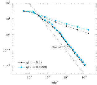
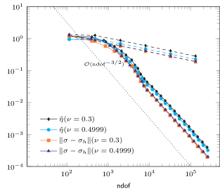
The material parameters $\lambda,\mu$ are given by the formulas $\lambda=E\nu/((1+\nu)(1-2\nu))$ and $\mu=E/(2(1+\nu))\to\infty$ as $\nu\to 1/2$ with the default Young’s modulus $E=10^{5}$ and the Poisson ratio $\nu=0.4999$. The only exceptions of those parameters are in Figure 2.b and Figure 5.b, where $\nu=0.4999$ is displayed as well as numerical results for $\nu=0.3$ for a comparison.

Adaptive computations utilize the refinement indicator

$$\eta^{2}(T) \coloneqq\|h_{T}(f+\mathrm{div}\,\sigma_{h})\|_{L^{2}(T)}^{2}+\mu^{2}\|\varepsilon(\mathcal{A}u_{h})-\varepsilon_{h}u_{h}\|_{L^{2}(T)}^{2}$$

(5.1) $$\qquad+\sum_{F\in\mathcal{F}(T)\cap\mathcal{F}(\Omega)}h_{F}\|[\sigma_{h}]_{F}\nu_{F}\|_{L^{2}(F)}^{2}+\sum_{F\in\mathcal{F}(T)\cap\mathcal{F}_{\mathrm{N}}}h_{F}\|g-\sigma_{h}\nu_{F}\|_{L^{2}(F)}^{2}$$

for $T\in\mathcal{T}\in\mathbb{T}$ arising from the error estimator (1.3) with the average $\mathcal{A}u_{h}$ of $\mathcal{R}u_{h}$. A standard adaptive loop [19] with the Dörfler marking strategy determines a subset $\mathcal{M}$ of minimal cardinality such that

$$\sum_{T\in\mathcal{T}}\eta^{2}(T)\leq\frac{1}{2}\sum_{T\in\mathcal{M}}\eta^{2}(T).$$

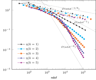
The convergence history plots display the quantities of interest against the number of degrees of freedom $\mathtt{ndof}$ in a log-log plot. (Recall the scaling $\mathtt{ndof}\approx h_{\mathrm{max}}^{-2}$ for uniform meshes in 2D.) Solid lines indicate adaptive, while dashed lines are associated with uniform mesh refinements.

The implementation of the solver for the discrete problem (2.15) has been carried out in MATLAB in an extension to the short MATLAB programs [1]. The integrals of polynomials are exactly computed while numerical quadrature is utilized for the integration of non-polynomial functions, e.g., in the computation of the errors.

Figure 1. (a) Cook’s membrane and (b) convergence history plot of $\eta$ for $k=1,\dots,5$ in Subsection 5.2

Figure 2. (a) Adaptive triangulation into 592 triangles generated with $k=2$ and (b) comparison between different $\nu$ with $k=2$ in Subsection 5.2

5.2. Cook’s membrane

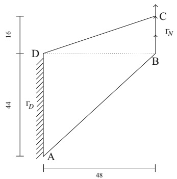
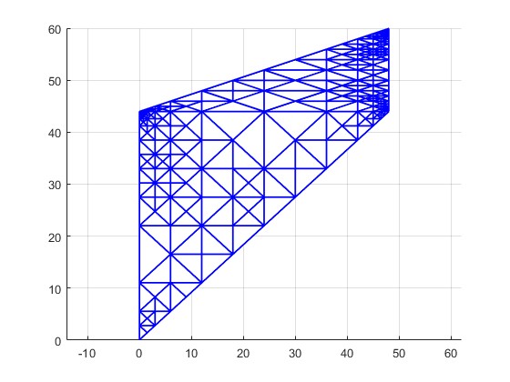
The tapered panel $\Omega\coloneqq\mathrm{conv}\{(0,0),(48,44),(48,60)$, $(0,44)\}$ of Figure 1.a (courtesy from [12]) is clamped on the left-hand side $\Gamma_{\mathrm{D}}\coloneqq\mathrm{conv}\{(0,0),(0,44)\}$, subjected to the shear load $g=(0,1)$ in vertical direction on the right side $\{48\}\times[44,60]$, and traction free elsewhere. The initial triangulation $\mathcal{T}_{0}$ consists of two triangles by partition of $\Omega$ along the line $[0,48]\times\{44\}$. Figure 1.b displays the suboptimal convergence rate $1/3$ for the error estimator $\eta$ with all displayed polynomial degrees $k=1,\dots,5$. The adaptive algorithm locally refines towards the four corners of the domain $\Omega$ in Figure 2.a for $k=2$ and $|\mathcal{T}|=592$ and recovers the optimal convergence rates $(k+1)/2$ for $\eta$ in Figure 1.b.

Figure 3. (a) Rotated L-shaped domain and (b) convergence history plot of $\widetilde{\eta}$ for $k=1,\dots,5$ in Subsection 5.3

Figure 4. (a) Convergence history plot of $\|\sigma-\sigma_{h}\|$ for $k=1,\dots,5$ and (b) adaptive triangulation into 545 triangles generated with $k=2$ in Subsection 5.3

Figure 5. (a) Efficiency index $\widetilde{\eta}/\|\sigma-\sigma_{h}\|$ for $k=1,\dots,5$ and (b) comparison between different $\nu$ with $k=2$ in Subsection 5.3

5.3. L-shaped domain

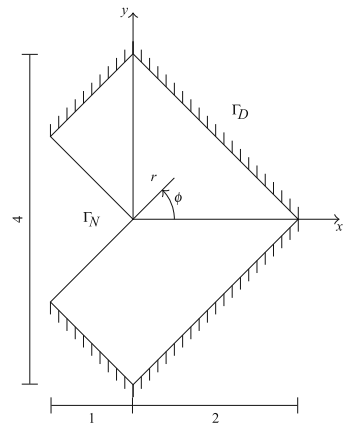
The rotated L-shaped domain $\Omega=\mathrm{conv}\{(0,0),(-1,-1)$, $(0,-2),(1,-1),(2,0),(0,2),(-1,1)\}$ with displayed Dirichlet and Neumann boundary parts in Figure 3.a (courtesy from [12]) allows for the exact solution $u$ to (1.2), given in polar coordinates,

$$u_{r}(r,\varphi) =\frac{r^{\alpha}}{2\mu}(-(\alpha+1)\cos((\alpha+1)\varphi)+(C_{2}-\alpha-1)C_{1}\cos((\alpha-1)\varphi)),$$

$$u_{\varphi}(r,\varphi) =\frac{r^{\alpha}}{2\mu}((\alpha+1)\sin((\alpha+1)\varphi)+(C_{2}+\alpha-1)C_{1}\sin((\alpha-1)\varphi))$$

with the first root $\alpha=0.544483736782$ of $\alpha\sin(2\omega)+\sin(2\omega\alpha)=0$ for $\omega=3\pi/4$, $C_{1}=-\cos((\alpha+1)\omega)/\cos((\alpha-1)\omega)$, and $C_{2}=2(\lambda+2\mu)/(\lambda+\mu)$ [9]. The applied force $f=0$ and $g=0$ vanish but inhomogeneous Dirichlet boundary conditions apply with $\|\sigma-\sigma_{h}\|\lesssim\widetilde{\eta}$ from (4.17). (In particular, the local contributions of $\mathrm{osc}(u_{\mathrm{D}},\mathcal{F}_{\mathrm{D}})^{2}$ are added to (5.1).)

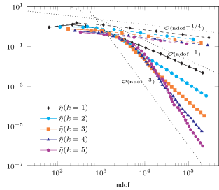
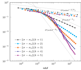
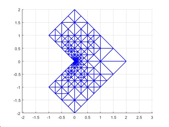
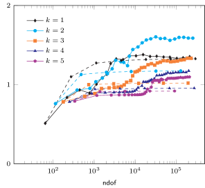
Figure 3.b and Figure 4.a display convergence rates $1/4$ for $\widetilde{\eta}$ and $\|\sigma-\sigma_{h}\|$ on uniform triangulations. Adaptive computations refine towards the singularity at the origin as shown in Figure 4.b and recover the optimal convergence rates $(k+1)/2$ for $\widetilde{\eta}$ and $\|\sigma-\sigma_{h}\|$ with all displayed polynomial degrees $k$. In this example, the efficiency indices are in the range 0.5 to 2 and do not increase with larger $k$, cf. Figure 5.a.

5.4. Conclusions

In all three numerical examples, the a posteriori error estimator $\eta$ is reliable, efficient, and $\lambda$-robust. This allows for the approximation of the Stokes equations in the incompressible limit as $\lambda\to\infty$. The adaptive algorithm driven by the local contributions of $\eta$ recovers the optimal convergence rates for the approximation of singular solutions and enables higher order convergence rates in typical computational benchmarks. A comparison with the results for $\nu=0.3$ displayed in Figure 2.b and Figure 5.b verifies empirically the $\lambda$-robustness of the method.

References

- [1] Jochen Alberty, Carsten Carstensen and Stefan A. Funken “Remarks around 50 lines of Matlab: short finite element implementation” In Numer. Algorithms 20.2-3, 1999, pp. 117–137 DOI: 10.1023/A:1019155918070
- [2] Fleurianne Bertrand, Carsten Carstensen, Benedikt Gräßle and Ngoc Tien Tran “Stabilization-free HHO a posteriori error control” In Numer. Math. 154.3-4, 2023, pp. 369–408 DOI: 10.1007/s00211-023-01366-8
- [3] Daniele Boffi, Franco Brezzi and Michel Fortin “Mixed finite element methods and applications” Springer, Heidelberg, 2013 DOI: 10.1007/978-3-642-36519-5
- [4] Michele Botti, Daniele A. Di Pietro and Alessandra Guglielmana “A low-order nonconforming method for linear elasticity on general meshes” In Comput. Methods Appl. Mech. Engrg. 354, 2019, pp. 96–118 DOI: 10.1016/j.cma.2019.05.031
- [5] Michele Botti, Daniele A. Di Pietro and Pierre Sochala “A hybrid high-order method for nonlinear elasticity” In SIAM J. Numer. Anal. 55.6, 2017, pp. 2687–2717 DOI: 10.1137/16M1105943
- [6] Dietrich Braess “Finite elements” Theory, fast solvers, and applications in elasticity theory, Translated from the German by Larry L. Schumaker Cambridge University Press, Cambridge, 2007, pp. xviii+365 DOI: 10.1017/CBO9780511618635
- [7] Susanne C. Brenner “Korn’s inequalities for piecewise vector fields” In Math. Comp. 73.247, 2004, pp. 1067–1087 DOI: 10.1090/S0025-5718-03-01579-5
- [8] Susanne C. Brenner and Li-Yeng Sung “Linear finite element methods for planar linear elasticity” In Math. Comp. 59.200, 1992, pp. 321–338 DOI: 10.2307/2153060
- [9] C. Carstensen, M. Eigel and J. Gedicke “Computational competition of symmetric mixed FEM in linear elasticity” In Comput. Methods Appl. Mech. Engrg. 200.41-44, 2011, pp. 2903–2915 DOI: 10.1016/j.cma.2011.05.013
- [10] C. Carstensen and N. Nataraj “A priori and a posteriori error analysis of the Crouzeix–Raviart and Morley FEM with original and modified right-hand sides” In Comput. Methods Appl. Math. 21.2, 2021, pp. 289–315 DOI: 10.1515/cmam-2021-0029
- [11] Carsten Carstensen and Georg Dolzmann “A posteriori error estimates for mixed FEM in elasticity” In Numer. Math. 81.2, 1998, pp. 187–209 DOI: 10.1007/s002110050389
- [12] Carsten Carstensen, Dietmar Gallistl and Joscha Gedicke “Residual-based a posteriori error analysis for symmetric mixed Arnold-Winther FEM” In Numer. Math. 142.2, 2019, pp. 205–234 DOI: 10.1007/s00211-019-01029-7
- [13] Carsten Carstensen and Norbert Heuer “A fractional-order trace-dev-div inequality” In arXiv:2403.01291, 2024
- [14] Carsten Carstensen, Qilong Zhai and Ran Zhang “A skeletal finite element method can compute lower eigenvalue bounds” In SIAM J. Numer. Anal. 58.1, 2020, pp. 109–124 DOI: 10.1137/18M1212276
- [15] Matteo Cicuttin, Alexandre Ern and Nicolas Pignet “Hybrid high-order methods—a primer with applications to solid mechanics”, Springer Briefs in Mathematics Springer, Cham, 2021, pp. viii+136 DOI: 10.1007/978-3-030-81477-9
- [16] Daniele A. Di Pietro and Alexandre Ern “A hybrid high-order locking-free method for linear elasticity on general meshes” In Comput. Methods Appl. Mech. Engrg. 283, 2015, pp. 1–21 DOI: 10.1016/j.cma.2014.09.009
- [17] Daniele A. Di Pietro, Alexandre Ern and Simon Lemaire “An arbitrary-order and compact-stencil discretization of diffusion on general meshes based on local reconstruction operators” In Comput. Methods Appl. Math. 14.4, 2014, pp. 461–472 DOI: 10.1515/cmam-2014-0018
- [18] Daniele Antonio Di Pietro and Jérôme Droniou “The hybrid high-order method for polytopal meshes” Design, analysis, and applications 19, MS&A. Modeling, Simulation and Applications Springer, 2020, pp. xxxi+525 DOI: 10.1007/978-3-030-37203-3
- [19] Willy Dörfler “A convergent adaptive algorithm for Poisson’s equation” In SIAM J. Numer. Anal. 33.3, 1996, pp. 1106–1124
- [20] Alexandre Ern and Pietro Zanotti “A quasi-optimal variant of the hybrid high-order method for elliptic partial differential equations with loads” In IMA J. Numer. Anal. 40.4, 2020, pp. 2163–2188 DOI: 10.1093/imanum/drz057
- [21] Vivette Girault and Pierre-Arnaud Raviart “Finite element methods for Navier-Stokes equations” Theory and algorithms Springer-Verlag, Berlin, 1986 DOI: 10.1007/978-3-642-61623-5
- [22] Joseph M. Maubach “Local bisection refinement for -simplicial grids generated by reflection” In SIAM J. Sci. Comput. 16.1, 1995, pp. 210–227 DOI: 10.1137/0916014
- [23] Andreas Rössle “Corner singularities and regularity of weak solutions for the two-dimensional Lamé equations on domains with angular corners” In J. Elasticity 60, 2000, pp. 57–75
- [24] L. Ridgway Scott and Shangyou Zhang “Finite element interpolation of nonsmooth functions satisfying boundary conditions” In Math. Comp. 54.190, 1990, pp. 483–493 DOI: 10.2307/2008497
- [25] Rob Stevenson “The completion of locally refined simplicial partitions created by bisection” In Math. Comput. 77.261, 2008, pp. 227–241
- [26] Andreas Veeser and Pietro Zanotti “Quasi-optimal nonconforming methods for symmetric elliptic problems. II—Overconsistency and classical nonconforming elements” In SIAM J. Numer. Anal. 57.1, 2019, pp. 266–292 DOI: 10.1137/17M1151651
- [27] Andreas Veeser and Pietro Zanotti “Quasi-optimal nonconforming methods for symmetric elliptic problems. III—Discontinuous Galerkin and other interior penalty methods” In SIAM J. Numer. Anal. 56.5, 2018, pp. 2871–2894 DOI: 10.1137/17M1151675
- [28] L. Veiga et al. “Adaptive VEM: stabilization-free a posteriori error analysis and contraction property” In SIAM J. Numer. Anal. 61.2, 2023, pp. 457–494 DOI: 10.1137/21M1458740
- [29] Rüdiger Verfürth “A posteriori error estimation techniques for finite element methods” Oxford University Press, Oxford, 2013 DOI: 10.1093/acprof:oso/9780199679423.001.0001