Quantum conjugate gradient method using the positive-side quantum eigenvalue transformation

Kiichiro Toyoizumi Department of Applied Physics and Physico-Informatics, Keio University, Hiyoshi 3-14-1, Kohoku-ku, Yokohama, 223-8522, Japan toyoizumi@ppl.appi.keio.ac.jp    Kaito Wada Department of Applied Physics and Physico-Informatics, Keio University, Hiyoshi 3-14-1, Kohoku-ku, Yokohama, 223-8522, Japan    Naoki Yamamoto Department of Applied Physics and Physico-Informatics, Keio University, Hiyoshi 3-14-1, Kohoku-ku, Yokohama, 223-8522, Japan Quantum Computing Center, Keio University, Hiyoshi 3-14-1, Kohoku-ku, Yokohama, 223-8522, Japan    Kazuo Hoshino Department of Applied Physics and Physico-Informatics, Keio University, Hiyoshi 3-14-1, Kohoku-ku, Yokohama, 223-8522, Japan
Abstract

Quantum algorithms are still challenging to solve linear systems of equations on real devices. This challenge arises from the need for deep circuits and numerous ancilla qubits. We introduce the quantum conjugate gradient (QCG) method using the quantum eigenvalue transformation (QET). The circuit depth of this algorithm depends on the square root of the coefficient matrix’s condition number $\kappa$, representing a square root improvement compared to the previous quantum algorithms, while the total query complexity worsens. The number of ancilla qubits is constant, similar to other QET-based algorithms. Additionally, to implement the QCG method efficiently, we devise a QET-based technique that uses only the positive side of the polynomial (denoted by $P(x)$ for $x\in[0,1]$). We conduct numerical experiments by applying our algorithm to the one-dimensional Poisson equation and successfully solve it. Based on the numerical results, our algorithm significantly improves circuit depth, outperforming another QET-based algorithm by three to four orders of magnitude.

1 Introduction

1.1 Background

Linear systems of equations are found in various fields, such as physics, engineering, and machine learning. The standard method for solving large systems involves using a computer. However, solving these systems demands a significant amount of computation time because the time complexity of the standard algorithms scales as $\mathrm{poly}(N)$ for the system size $N$. A promising alternative approach is the use of a quantum computer. The first quantum algorithm for solving linear systems of equations is the Harrow-Hassidim-Lloyd (HHL) algorithm [1]. Under specific conditions, the HHL algorithm achieves an exponential speedup over classical algorithms, such as the conjugate gradient (CG) method [2, 3]. This discovery has led to various quantum linear system algorithms (QLSAs) [4, 5, 6, 7, 8, 9, 10].

However, the practical implementation of these algorithms on real devices is anticipated to be difficult for the next few decades. This challenge arises due to the need for deep circuits and numerous ancilla qubits. For instance, the HHL algorithm, relying on quantum phase estimation [12], requires deep circuits with many controlled time evolution operators. The HHL algorithm achieves linear dependence of circuit depth on the condition number $\kappa$ of a given matrix through variable time amplitude amplification [4]. However, implementing this algorithm on real devices remains difficult. Moreover, because of the need to store the eigenvalues of the matrix in ancilla qubits with a certain precision, the number of ancilla qubits depends on $\kappa$ and a desired precision $\varepsilon$, resulting in numerous ancilla qubits. An effective approach to avoid this dependence is using the quantum singular-value transformation (QSVT) [8].

The QSVT is a quantum algorithm that calculates a polynomial of a given matrix embedded in a larger unitary matrix. Notably, the QSVT provides a unified approach to major quantum algorithms, such as the Grover search [13], quantum phase estimation, quantum walks [14], Hamiltonian simulation [15, 16], and matrix inversion. In the QSVT-based QLSAs [8, 9, 10], the number of ancilla qubits is constant, regardless of both $\kappa$ and $\varepsilon$. However, reducing the circuit depth of these algorithms is desirable in terms of their implementation on real devices. Therefore, our goal is to present a QSVT-based QLSA with shallow circuits.

1.2 Contribution of this paper

We define some terms and notations to describe the contributions of this paper. Let $A$ and $\ket{b}$ be a given invertible $N\times N$ matrix and $N$-dimensional vector; then $\ket{x}$ is the solution of a linear system of equations $A\ket{x}=\ket{b}$. Note that the vectors $\ket{x}$ and $\ket{b}$ are not normalized. The condition number of $A$ is defined by $\kappa=\|A\|\|A^{-1}\|$, where $\|\cdot\|$ represents the $L_{2}$ norm in this paper. Suppose that $A$ can be efficiently accessed through an oracle or a block encoding (defined in Sec.2.1) and $\ket{b}/\|\ket{b}\|$ can be efficiently prepared through an oracle. Then the QLSA is a quantum algorithm that produces a quantum state $\ket{\tilde{x}}/\|\ket{\tilde{x}}\|$ such that $\|\ket{x}-\ket{\tilde{x}}\|\leq\varepsilon$. The circuit depth is defined by the number of queries to the block encoding of $A$ in the QSVT framework or the oracle to access elements of $A$ in others. The maximum circuit depth is the highest depth among all the circuits in the algorithm. Total query complexity is the overall number of queries to obtain the state $\ket{\tilde{x}}/\|\ket{\tilde{x}}\|$, expressed as the sum of the products of the circuit depths and the number of circuit runs. We use the asymptotic notation $O(t\mathrm{polylog}(t))=\tilde{O}(t)$. The $\varepsilon$ approximation of a function $f$ to $g$ on the domain $I$ is denoted by the inequality $\max_{x\in I}|g(x)-f(x)|\leq\varepsilon.$

The CG method [2, 3] is a well-established classical algorithm for solving a linear system of equations involving a positive definite Hermitian matrix $A$. In this method, vectors are represented as the product of the polynomial $P(A)$ and the initial vector $\ket{b}$. Based on this observation, we introduce the quantum conjugate gradient (QCG) method using the quantum eigenvalue transformation (QET), corresponding to the QSVT for a Hermitian matrix. This algorithm iteratively constructs new polynomials and produces corresponding states in each iteration. In contrast, the QSVT-based QLSA [8, 10] constructs a polynomial directly approximating $A^{-1}$. Thus, we call this algorithm the QLSA using the direct QSVT. Table LABEL:tb:comparison_of_QLSAs compares the QLSAs regarding the maximum circuit depth, the number of ancilla qubits, and the total query complexity.

Our algorithm achieves a square-root improvement for $\kappa$ in the maximum circuit depth. This enhancement stems from the convergence of the CG method. In the CG method, the number of iterations required to meet the convergence criterion scales as $m=O\left(\sqrt{\kappa}\log\left(\frac{\kappa\|\ket{b}\|}{\|A\|\varepsilon}\right)\right)$ The maximum degree of the polynomial $P(A)$ is represented as $m+1$. Since our algorithm estimates inner products using two polynomials, the maximum circuit depth is $2(m+1)=O\left(\sqrt{\kappa}\log\left(\frac{\kappa\|\ket{b}\|}{\|A\|\varepsilon}\right)\right)$. Furthermore, the number of ancilla qubits remains constant, independent of both $\kappa$ and $\varepsilon$, because the QET framework formulates our algorithm. Therefore, our algorithm achieves shallow circuits with a constant number of ancilla qubits.

Note that the total query complexity of our algorithm is less favorable compared to that of other QLSAs. This is due to the necessity of numerous circuit runs to estimate inner products using swap tests [17]. This trade-off implies that our algorithm achieves shallow circuits at the expense of increasing the number of circuit runs. However, the total query complexity is derived as a worst case and can be improved by optimizing the number of circuit runs and the precision for estimating inner products.

We show that the polynomials’ maximum absolute values of the negative side ($x\in[-1,0]$) can grow significantly in specific problems where the QCG method is applied. Addressing this growth requires amplitude amplification that demands an enormous cost in the previous QET framework. To overcome this challenge, we introduce a novel technique named positive-side QET. This technique allows us to use only the positive side ($x\in[0,1]$) of a polynomial for a positive semidefinite Hermitian matrix $A$. Importantly, this technique requires neither amplitude amplification nor additional cost, assuming the block encoding of $A^{\prime}=2A-I$ exists. The QCG method can be implemented efficiently by integrating this technique. Additionally, we elaborate on the explicit construction of this block encoding to ensure the applicability of the positive-side QET. In the QET framework, certain constraints impose limitations on the range of applicable polynomials. Specifically, the absolute value of polynomials for $x\in[-1,1]$ must not exceed $1$. Accordingly, polynomials that meet the constraints have been chosen, such as the Chebyshev polynomial and approximate polynomials of trigonometric and sign functions. [8, 10]. The positive-side QET can efficiently handle polynomials with an enormous absolute value on the negative side. Importantly, the application of this technique is not limited to the QCG method; it can be applied more broadly. Therefore, this technique broadens the scope of applicable polynomials in the QET framework.

We apply the QCG method using the positive-side QET to solve the one-dimensional Poisson equation for testing. We achieve successful solutions using the Statevector Simulator provided by Qiskit [18]. Notably, our algorithm’s maximum circuit depth is significantly smaller (three to four orders) than that of the QLSA using the direct QSVT [10]. Thus, we numerically demonstrate that our algorithm exhibits shallow circuits.

1.3 Related works

The QLSAs have evolved toward improving their dependence on $\kappa$ and $\varepsilon$. The total query complexity of the HHL algorithm [1] is $\tilde{O}(\kappa^{2}/\varepsilon)$. For any $\delta>0$, a QLSA with cost $O(\kappa^{1-\delta})$ would imply BQP=PSPACE. Therefore, the lower bound of the QLSA’s total query complexity is regarded as $\Omega(\kappa)$. Note that this fact is consistent with the square root dependence for $\kappa$ of our algorithm’s maximum circuit depth because the dependence of the total query complexity is superlinear. Ambainis developed variable time amplitude amplification (VTAA) to improve the dependence from $\kappa^{2}$ to $\kappa$ [4]; however, the $1/\varepsilon$-dependence remains polynomial. In [5], the authors reduced this dependence to log-polynomial using the method for implementing linear combinations of unitaries (LCU). The LCU approach requires $O(\log d)$ ancilla qubits, where $d$ is the degree of approximation. Since this approach utilizes an approximation of $1/x$, the number of ancilla qubits depends on $\kappa$ and $\varepsilon$. In [6], the authors presented the QLSA for dense matrices by combining the HHL with the quantum singular-value estimation (QSVE) [19]. In [8], the authors introduced the QSVT and explained the QLSA in this framework. The details were provided in [10]. The maximum circuit depth of this algorithm without amplitude amplification scales as $O(\kappa\log(\kappa/\varepsilon))$, which represents a better scaling compared to other QLSAs [4, 5, 6, 7, 9]. However, in the worst case, the total query complexity with amplitude amplification scales as $O(\kappa^{2}\log(\kappa/\varepsilon))$. In [9], the authors proposed eigenstate filtering by the QSVT. They reduced the dependence from $\kappa^{2}$ to $\kappa$ in the total query complexity by combining this method and quantum adiabatic computing [20] or quantum Zeno effect [21]. Specifically, the query complexity of the method with the quantum Zeno effect is $O(\kappa\left[\log(\kappa)\log\log(\kappa)+\log(1/\varepsilon)\right])$. The number of ancilla qubits of these QSVT-based QLSAs is constant, regardless of both $\kappa$ and $\varepsilon$.

The QCG method was initially discussed by Shao [7]. The author also focused on the representation of vectors in the CG method, expressed as the product of the polynomial $P(A)$ and the initial vector $\ket{b}$. A technique based on the quantum phase estimation was developed to prepare an approximate linear combination of two quantum states. This technique is repeatedly applied to construct the polynomial, resulting in the number of ancilla qubits dependent on the polynomial degree. The maximum degree is determined by $\kappa$ and $\varepsilon$; therefore, the number of ancilla qubits depends on both. Moreover, the scaling for $\kappa$ of the maximum circuit depth can be superlinear. Consequently, Shao’s QCG method does not achieve the shallow circuit with constant ancilla qubits.

The CG method is a form of the Krylov subspace method. Various quantum Krylov subspace methods have been developed [22, 23, 24, 25, 26, 27]. These algorithms are designed to address eigenvalue problems, particularly finding the smallest eigenvalue rather than linear systems of equations. In these algorithms, a Hamiltonian eigenvalue problem is transformed into a generalized eigenvalue problem. The resolution of these problems involves the evaluation of inner products and expectation values of states in the Krylov subspace. The states are generated through operations such as the real-time evolution operators [22, 24, 25, 26], the imaginary-time evolution operators [23], or the Chebyshev polynomial [27].

2 Preliminary

2.1 Quantum eigenvalue transformation

The quantum eigenvalue transformation [8, 10, 28] is a quantum algorithm for calculating a polynomial transformation $P(A)$, where $P$ is a polynomial, and $A$ is a Hermitian matrix embedded in a larger unitary matrix. The QET is derived from quantum signal processing [29, 28] and consists of three steps: input, processing, and output. The input involves a block encoding, representing a square matrix as the upper left block of a unitary matrix. The block encoding is defined as follows. Let $n_{s}$ and $n_{a}$ be the number of the system and ancilla qubits. Let $A$ be a Hermitian matrix acting on $n_{s}$ qubits and $U_{A}$ be a unitary matrix acting on $n_{a}+n_{s}$ qubits. Then for a subnormalization factor $\alpha>0$ and an error $\varepsilon>0$, $U_{A}$ is called $(\alpha,n_{a},\varepsilon)$ block encoding of $A$ if

$$\left\|A-\alpha(\bra{0}_{a}\otimes I_{s})U_{A}(\ket{0}_{a}\otimes I_{s})\right\|\leq\varepsilon,$$ (1)

where $\ket{0}_{a}=\ket{0}^{\otimes n_{a}}$ and $I_{s}$ is an identity matrix acting on $n_{s}$ qubits. Note that we necessarily have $\|A\|\leq\alpha+\varepsilon$ because $\|U\|=1$.

The QET processes the input $U_{A}$ using the following sequence with $d+1$ real parameters $\Phi=(\phi_{0},\phi_{1},\dots,\phi_{d})$, known as a phase factor: For even $d$,

$$U_{\Phi}\equiv e^{i\phi_{0}\Pi}\prod_{k=1}^{d/2}\left(U_{A}^{\dagger}e^{i\phi_{2k-1}\Pi}U_{A}e^{i\phi_{2k}\Pi}\right),$$ (2)

for odd $d$,

$$U_{\Phi}\equiv e^{i\phi_{0}\Pi}U_{A}e^{i\phi_{1}\Pi}\prod_{k=1}^{(d-1)/2}\left(U_{A}^{\dagger}e^{i\phi_{2k}\Pi}U_{A}e^{i\phi_{2k+1}\Pi}\right),$$ (3)

where $\Pi=2\ket{0}_{a}\bra{0}-I$. The operator $e^{i\phi\Pi}$ changes the input using the angle of the phase factor.

The main result of the QET is that the output is represented as $(1,n_{a}+1,0)$ block encoding of $P(A/\alpha)$ if $U_{A}$ is $(\alpha,n_{a},\varepsilon)$ block encoding of $A$ and a degree-$d$ real polynomial $P\in\mathbb{R}[x]$ satisfies the conditions

  • (i)

    $P$ has parity $d\bmod{2}$,

  • (ii)

    $\forall x\in[-1,1]:|P(x)|\leq 1$.

The phase factor $\Phi$ for the even or odd polynomial can be calculated classically in time $O(\mathrm{poly}(d))$ from the polynomial coefficients [30, 31, 32, 33, 34, 35]. Figure 1 illustrates the QET circuits for a degree-$d$ real polynomial $P$ with definite parity, representing $(1,n_{a}+1,0)$ block encoding of $P(A/\alpha)$. If $P$ is a polynomial that $\varepsilon$ approximates a given function $f$ for $x\in[-1,1]$, then the circuit becomes $(1,n_{a}+1,\varepsilon)$ block encoding of $f(A/\alpha)$. The QET circuit features the gate $S_{1}(\phi)$ shown in Fig. 2, which has one angle of the phase factor. This gate is essentially equal to the processing operator $e^{i\phi\Pi}$ in Eqs. (2) and (3). Since the circuit includes just $d$ queries to $U_{A}$, the polynomial degree is regarded as a metric for the QET circuit’s depth.

Refer to caption

(a)

Refer to caption

(b)

Figure 1: The QET circuits for a degree-$d$ real polynomial with definite parity: (a) For an even polynomial and (b) for an odd polynomial.
Refer to caption
Figure 2: The gate $S_{1}(\phi)$. For $b=\{0,1\}$, this gate is expressed as $S_{1}(\phi)=\sum_{b}\ket{b}\bra{b}\otimes e^{(-1)^{b}i\phi\Pi}$. The anti-controlled NOT gate is controlled by $n_{a}$ qubits.

2.1.1 Approximate polynomials of sign and rectangular functions

Let $\delta\in(-1,1),\Delta>0$, and $\varepsilon\in(0,\sqrt{8/e\pi}]$. According to the results of [36, 37], there exists a polynomial $P_{\delta,\Delta,\varepsilon}^{\mathrm{sgn}}(x)$ that $\varepsilon$ approximates a sign function

$$\mathrm{sgn}(x-\delta)=\begin{cases}-1&x<\delta\\ 0&x=\delta\\ 1&x>\delta,\end{cases}$$ (4)

for $x\in[-1,\delta-\frac{\Delta}{2}]\cup[\delta+\frac{\Delta}{2},1]$ with the degree

$\displaystyle d_{\mathrm{sgn}}(\delta,\Delta,\varepsilon)$
$\displaystyle=2\left\lceil\frac{16(1+|\delta|)k}{\sqrt{\pi}\varepsilon}\exp\left[-\frac{1}{2}W\left(\frac{512}{\pi\varepsilon^{2}e^{2}}\right)\right]\right\rceil+1$
$\displaystyle=O\left(\frac{1+|\delta|}{\Delta}\log(1/\varepsilon)\right),$ (5)

where $W$ is the Lambert $W$ function and

$$k(\Delta,\varepsilon)=\frac{1}{\Delta}\sqrt{2\ln\left(\frac{8}{\pi\varepsilon^{2}}\right)}.$$ (6)
Refer to caption

(a)

Refer to caption

(b)

Figure 3: The QET circuits for a degree-$d$ real polynomial without definite parity: (a) For even $d$. The angle $\vec{\phi}_{j}$ is defined as $\vec{\phi}_{j}=(\phi_{j}^{(\mathrm{even})},\phi_{j-1}^{(\mathrm{odd})})$ for $j=1,2,\dots,d$. (b) For odd $d$. The angle $\vec{\phi}_{j}$ is defined as $\vec{\phi}_{j}=(\phi_{j-1}^{(\mathrm{even})},\phi_{j}^{(\mathrm{odd})})$ for $j=1,2,\dots,d$.
Refer to caption
Figure 4: The gate $S_{2}(\vec{\phi})$. For $\vec{\phi}=(\phi^{(0)},\phi^{(1)}),b=\{0,1\},$ and $c=\{0,1\}$, this gate is expressed as $S_{2}(\vec{\phi})=\sum_{b,c}\ket{cb}\bra{cb}\otimes e^{(-1)^{b}i\phi^{(c)}\Pi}$.

We define a rectangular function in two forms: Open and closed rectangular functions. For $\delta\in(0,1)$, an open rectangular function is defined by

$$\mathrm{rect}(x)=\begin{cases}0&|x|<\delta\\ \frac{1}{2}&|x|=\delta\\ 1&\delta<|x|\leq 1.\end{cases}$$ (7)

This function is represented as a linear combination of two sign functions

$$\mathrm{rect}(x)=1+\frac{1}{2}\left(\mathrm{sgn}(x-\delta)+\mathrm{sgn}(-x-\delta)\right).$$ (8)

Therefore, for $\Delta>0,\varepsilon\in(0,1)$, there exists a polynomial $P_{\delta,\Delta,\varepsilon}^{\mathrm{rect}}(x)$ [10] that satisfies the inequalities

$\displaystyle\begin{split}\left|P_{\delta,\Delta,\varepsilon}^{\mathrm{rect}}(x)\right|&\leq\varepsilon,\quad x\in\left[-\delta+\frac{\Delta}{2},\delta-\frac{\Delta}{2}\right],\\ \left|1-P_{\delta,\Delta,\varepsilon}^{\mathrm{rect}}(x)\right|&\leq\varepsilon,\\ &x\in\left[-1,-\delta-\frac{\Delta}{2}\right]\cup\left[\delta+\frac{\Delta}{2},1\right],\\ \left|P_{\delta,\Delta,\varepsilon}^{\mathrm{rect}}(x)\right|&\leq 1,\quad x\in[-1,1]\end{split}$ (9)

with the degree

$$d_{\mathrm{rect}}(\delta,\Delta,\varepsilon)=d_{\mathrm{sgn}}\left(\delta,\Delta,\frac{\varepsilon}{2}\right)-1$$ (10)

On the other hand, a closed rectangular function is defined by

$$\mathrm{rect}(x)=\begin{cases}1&|x|<\delta\\ \frac{1}{2}&|x|=\delta\\ 0&\delta<|x|\leq 1.\end{cases}$$ (11)

This function is also represented as a linear combination of two sign functions

$$\mathrm{rect}(x)=\frac{1}{2}\left(\mathrm{sgn}(x+\delta)+\mathrm{sgn}(-x+\delta)\right).$$ (12)

Thus, there exists a polynomial that $\varepsilon$ approximates the closed rectangular function with the degree in Eq. (10).

2.1.2 General polynomial

In specific problems, we encounter polynomials that do not satisfy conditions (i) and (ii). This indicates a lack of definite parity and the maximum absolute value within the domain $[-1,1]$ exceeding 1. Such polynomials were discussed in [32]. Here, we explicitly describe implementing a general polynomial through the QET.

Let $U_{A}$ be a $(\alpha,n_{a},0)$ block encoding of $A$ and $P\in\mathbb{R}[x]$ be a real polynomial $P(x)=\sum_{j=0}^{d}c_{j}x^{j}$. We divide it into even and odd polynomials

$\displaystyle\begin{split}P_{d}^{\mathrm{even}}(x)&=\sum_{l=0}^{\left\lceil\frac{d-1}{2}\right\rceil}c_{2l}x^{2l},\\ P_{d}^{\mathrm{odd}}(x)&=\sum_{l=1}^{\left\lceil\frac{d}{2}\right\rceil}c_{2l-1}x^{2l-1}.\end{split}$ (13)

To ensure that each polynomial satisfies condition (ii), we normalize them using the maximum absolute values

$\displaystyle\begin{split}C_{\max,d}^{\mathrm{even}}&=\max_{x\in[-1,1]}\left|P_{d}^{\mathrm{even}}(x)\right|,\\ C_{\max,d}^{\mathrm{odd}}&=\max_{x\in[-1,1]}\left|P_{d}^{\mathrm{odd}}(x)\right|.\end{split}$ (14)

The normalized constants must be the same because we create a linear combination of the normalized polynomials using two Hadamard gates; thus, we select the larger one

$$C_{\max,d}=\max\left\{C_{\max,d}^{\mathrm{even}},C_{\max,d}^{\mathrm{odd}}\right\}.$$ (15)

Since the polynomials normalized by this constant meet both conditions, we can compute the phase factors $\Phi^{(\mathrm{even})}$ and $\Phi^{(\mathrm{odd})}$ from the corresponding even and odd polynomials. Figure 3 shows the QET circuits for a real polynomial without definite parity, representing $(2C_{\max,d},n_{a}+2,0)$ block encoding of $P(A/\alpha)$. These circuits construct the block encodings of the linear combination of the normalized even and odd polynomials

$$\frac{\frac{1}{C_{\max,d}}\left[P_{d}^{\mathrm{even}}\left(\frac{A}{\alpha}\right)+P_{d}^{\mathrm{odd}}\left(\frac{A}{\alpha}\right)\right]}{2}=\frac{P\left(\frac{A}{\alpha}\right)}{2C_{\max,d}}$$ (16)

If $P$ is a polynomial that $\varepsilon$ approximates a given function $f$ for $x\in[-1,1]$, then the circuit becomes $(2C_{\max,d},n_{a}+2,\varepsilon)$ block encoding of $f(A/\alpha)$. The QET circuits have the gate $S_{2}(\vec{\phi})$ depicted in Fig. 4, which has two angles of the phase factors for even and odd polynomials. The number of queries to $U_{A}$ also equals the polynomial degree $d$.

2.2 QLSA using the direct QSVT

We present a review of the QLSA using the direct QSVT [10] to numerically compare the polynomial degrees of this algorithm and our algorithm in Sec. 4. Let $A$ be a positive definite Hermitian matrix such that $1\leq\|A\|\leq\alpha$ ($\|A\|\leq 1$ in [10]). Note that the results below can be readily generalized to general matrices; hence, we adopt the term QSVT. Let $\lambda_{\max}$ and $\lambda_{\min}$ be the maximum and minimum eigenvalues of $A$; then the condition number of $A$ is $\kappa=\|A\|\|A^{-1}\|=\lambda_{\max}/\lambda_{\min}\geq 1$. Since $1\leq\lambda_{\max}=\|A\|\leq\alpha$, $1/\kappa\leq\lambda_{\min}$. Therefore, the eigenvalues of $A/\alpha$ lie in the range $[\frac{1}{\kappa\alpha},1]$. Here we introduce a domain denoted by $D_{\eta}=[-1,-1/\eta]\cup[1/\eta,1]$ for $\eta>0$.

The inverse matrix is represented as $A^{-1}=\sum_{j}\frac{1}{\lambda_{j}}\ket{\lambda_{j}}\bra{\lambda_{j}}$, where $\{\ket{\lambda_{j}}\}$ is the eigenvectors of $A$. It can be rewritten as $A^{-1}=g(A)$, where $g(x)=\frac{1}{x}$. The magnitude of a polynomial is bounded by 1 in the QSVT framework. Thus, the goal is to construct a polynomial approximating a function $f(x)=\frac{1}{2\kappa\alpha x}$ for $x\in D_{\kappa\alpha}$. This polynomial comprises two polynomial approximations: $1/x$ and a rectangular function. As discussed in  [5, 10], for $0<\varepsilon<1/2$, the following odd polynomial $\varepsilon$ approximates $1/x$ for $D_{\kappa\alpha}$:

$\displaystyle P_{\kappa,\alpha,\varepsilon}^{1/x}(x)$
$\displaystyle=4\sum_{j=0}^{(d_{\mathrm{inv}}-1)/2}(-1)^{j}\left[\frac{\sum_{i=j+1}^{b}\binom{2b}{b+i}}{2^{2b}}\right]T_{2j+1}(x),$ (17)

where $T_{j}(x)$ is the $j$ th Chebyshev polynomial of the first kind, and $b$ and $d_{\mathrm{inv}}$ are

$$b(\kappa,\alpha,\varepsilon)=\left\lceil(\kappa\alpha)^{2}\log\left(\frac{2\kappa\alpha}{\varepsilon}\right)\right\rceil,$$ (18)
$\displaystyle d_{\mathrm{inv}}(\kappa,\alpha,\varepsilon)$
$\displaystyle=2\left\lceil\frac{1}{2}\sqrt{b(\kappa,\alpha,\varepsilon)\log\left(\frac{8b(\kappa,\alpha,\varepsilon)}{\varepsilon}\right)}\right\rceil+1$
$\displaystyle=O\left(\kappa\alpha\log\left(\frac{\kappa\alpha}{\varepsilon}\right)\right).$ (19)

Thus, $\frac{1}{2\kappa\alpha}P_{2\kappa,\alpha,\varepsilon}^{1/x}(x)$ is a polynomial $\frac{\varepsilon}{2\kappa\alpha}$ approximating $f(x)$ for $x\in D_{2\kappa\alpha}$.

The absolute value of the above polynomial can be greater than 1 for $x\in[\frac{-1}{2\kappa\alpha},\frac{1}{2\kappa\alpha}]$. Therefore, to ensure that the absolute value is bounded by 1, we must use the even function close to 1 for $x\in D_{\kappa\alpha}$ and close to 0 for $x\in[\frac{-1}{2\kappa\alpha},\frac{1}{2\kappa\alpha}]$. The domain $\left[\frac{-1}{\kappa\alpha},\frac{-1}{2\kappa\alpha}\right]\cup\left[\frac{1}{2\kappa\alpha},\frac{1}{\kappa\alpha}\right]$ is a transition region between these two regions. A function that satisfies the above requirements is the approximate polynomial of the open rectangular function for $\delta=\frac{3}{4\kappa\alpha},\Delta=\frac{1}{2\kappa\alpha}$ in Sec. 2.1.1. This polynomial satisfies the inequalities

$\displaystyle\begin{split}\left|P_{\frac{3}{4\kappa\alpha},\frac{1}{2\kappa\alpha},\varepsilon}^{\mathrm{rect}}(x)\right|&\leq\varepsilon,\quad x\in\left[-\frac{1}{2\kappa\alpha},\frac{1}{2\kappa\alpha}\right],\\ \left|1-P_{\frac{3}{4\kappa\alpha},\frac{1}{2\kappa\alpha},\varepsilon}^{\mathrm{rect}}(x)\right|&\leq\varepsilon,\quad x\in D_{\kappa\alpha},\\ \left|P_{\frac{3}{4\kappa\alpha},\frac{1}{2\kappa\alpha},\varepsilon}^{\mathrm{rect}}(x)\right|&\leq 1,\quad x\in[-1,1]\end{split}$ (20)

and the degree is

$$d_{\mathrm{rect}}\left(\frac{3}{4\kappa\alpha},\frac{1}{2\kappa\alpha},\varepsilon\right)=O\left(\kappa\alpha\log\left(1/\varepsilon\right)\right).$$ (21)

We build the following target polynomial by multiplying those two polynomials:

$$P_{\kappa,\alpha,\varepsilon}^{\mathrm{MI}}(x)\equiv\frac{1}{2\kappa\alpha}P_{2\kappa,\alpha,\frac{\varepsilon}{2}}^{1/x}(x)P_{\kappa,\alpha,\varepsilon^{\prime}}^{\mathrm{rect}}(x),$$ (22)

where

$$\varepsilon^{\prime}=\min\left(\frac{2\varepsilon}{5\kappa\alpha},\frac{\kappa\alpha}{2d_{\mathrm{inv}}(2\kappa,\alpha,\varepsilon/2)}\right)=O\left(\frac{\varepsilon}{\kappa\alpha}\right).$$ (23)

This polynomial satisfies $|P_{\kappa,\alpha,\varepsilon}^{\mathrm{MI}}(x)|\leq 1$ for $x\in[-1,1]$ and $\frac{\varepsilon}{2\kappa\alpha}$ approximates $f(x)$ for $x\in D_{\kappa\alpha}$:

$$\left|f(x)-P_{\kappa,\alpha,\varepsilon}^{\mathrm{MI}}(x)\right|\leq\frac{\varepsilon}{2\kappa\alpha}.$$ (24)

The polynomial degree is the sum of the degrees of the two polynomials

$\displaystyle d_{\mathrm{MI}}(\kappa,\alpha,\varepsilon)$ $\displaystyle=d_{\mathrm{inv}}\left(2\kappa,\alpha,\frac{\varepsilon}{2}\right)+d_{\mathrm{rect}}\left(\frac{3}{4\kappa\alpha},\frac{1}{2\kappa\alpha},\varepsilon^{\prime}\right)$
$\displaystyle=O\left(\kappa\alpha\log\left(\frac{\kappa\alpha}{\varepsilon}\right)\right).$ (25)

2.3 Conjugate gradient method

{algorithm}

[tbp] Conjugate gradient method.

0:  
1:  $\vec{r}_{0}=\vec{b}-A\vec{x}_{0},\vec{p}_{0}=\vec{r}_{0}$
2:  for $k=0,1,\ldots$ do
3:     $\alpha_{k}=\frac{\vec{r}_{k}\cdot\vec{r}_{k}}{\vec{p}_{k}\cdot A\vec{p}_{k}}$
4:     $\vec{x}_{k+1}=\vec{x}_{k}+\alpha_{k}\vec{p}_{k}$
5:     $\vec{r}_{k+1}=\vec{r}_{k}-\alpha_{k}A\vec{p}_{k}$
6:     if $\left\|\vec{r}_{k+1}\right\|\leq\varepsilon\|\vec{b}\|$ then
7:        STOP
8:     end if
9:     $\beta_{k}=\frac{\vec{r}_{k+1}\cdot\vec{r}_{k+1}}{\vec{r}_{k}\cdot\vec{r}_{k}}$
10:     $\vec{p}_{k+1}=\vec{r}_{k+1}+\beta_{k}\vec{p}_{k}$
11:  end for

The conjugate gradient method [2, 3] stands as a classical algorithm for solving a linear system of equations for a positive definite Hermitian matrix $A\in\mathbb{R}^{N\times N}$. This method belongs to a category of iterative techniques known as the Krylov subspace methods. The Krylov subspace is formed by vectors $\vec{v},A\vec{v},A^{2}\vec{v},\dots,A^{k-1}\vec{v}(k\leq N)$. Here $\vec{v}$ denotes a given $N$-dimensional vector. The vectors in the Krylov subspace are expressed as the product of the polynomial $P(A)$ and the initial vector $\vec{v}$. Therefore, the vectors of the CG method are also represented as the same product.

Algorithm 2.3 outlines the steps of the CG method. In each iteration, three vectors are generated: An approximate solution vector $\vec{x}_{k}$, a residual vector $\vec{r}_{k}=\vec{b}-A\vec{x}_{k}$, and a search vector $\vec{p}_{k}$. When $\vec{x}_{0}=0$, these vectors can be expressed as the product of the polynomial $P(A)$ and the initial vector $\vec{b}$ as follows:

$\displaystyle\begin{split}\vec{x}_{k}&=P_{x,k}(A)\vec{b}=\sum_{l=0}^{k-1}x_{k,l}A^{l}\vec{b},\\ \vec{r}_{k}&=P_{r,k}(A)\vec{b}=\sum_{l=0}^{k}r_{k,l}A^{l}\vec{b},\\ \vec{p}_{k}&=P_{p,k}(A)\vec{b}=\sum_{l=0}^{k}p_{k,l}A^{l}\vec{b}.\end{split}$ (26)

Based on Algorithm 2.3, the coefficients of those three polynomials are updated through the following equations: For $l=0,1,\dots,k+1$,

$\displaystyle\begin{split}x_{k+1,l}&=x_{k,l}+\alpha_{k}p_{k,l},\\ r_{k+1,l}&=r_{k,l}-\alpha_{k}p_{k,l-1},\\ p_{k+1,l}&=r_{k+1,l}+\beta_{k}p_{k,l},\end{split}$ (27)

where $p_{k,-1}=x_{k,k}=x_{k,k+1}=r_{k,k+1}=p_{k,k+1}=0$. In each iteration, $\vec{x}_{k}$, $\vec{r}_{k}$, and $\vec{p}_{k}$ are generated by constructing the polynomials using the coefficients determined by the above equations.

Refer to caption

(a)

Refer to caption

(b)

Figure 5: Plots of polynomials obtained by applying the CG method to the one-dimensional Poisson equation: (a) For $x\in[-1,1]$ and (b) for $x\in[0,1]$. The orange area represents the positive side ($x\in[0,1]$), and the blue area represents the negative side ($x\in[-1,0]$).

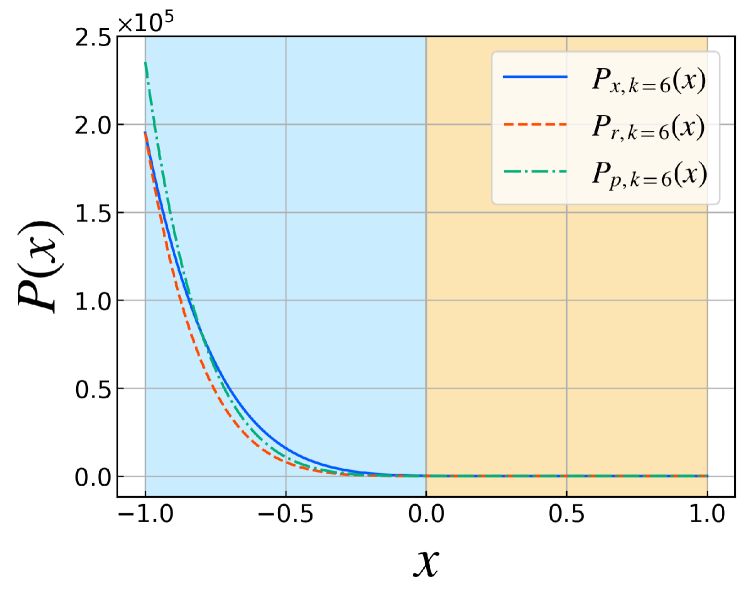
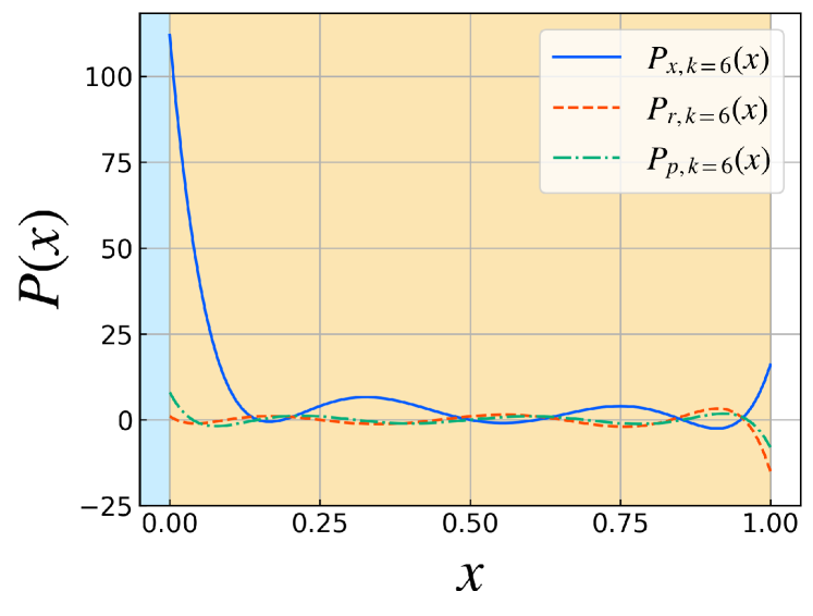
We address a potential problem concerning polynomials in the CG method. Figure 5 shows the polynomials obtained by applying this method to the one-dimensional Poisson equation (refer to Sec. 4 for more details). Figure 5(a) highlights the significant scaling of these polynomials for $x\in[-1,1]$, whereas Fig. 5(b) shows the relatively small scaling for $x\in[0,1]$. This enormous value arises because the polynomial coefficients are amplified due to $\alpha_{k}>1$ as iterations progress. The maximum absolute values on the positive side ($x\in[0,1]$) are smaller because the effects of the powers of the eigenvalues whose magnitudes are less than one and the huge coefficients cancel each other out. As explained in Sec. 2.1, the QET framework necessitates the normalization of polynomials by their maximum absolute values. Normalizing the polynomials in Fig. 5(a) using their maximum absolute values results in an extremely small success probability of the algorithm, indicating a significant increase in the query complexity. In Sec. 3.1 we provide a technique to address and overcome this challenge.

2.4 Swap test

We explain a method for computing the inner product of states multiplied by block encodings. This method is a slightly modified version of the swap test [17]. Let $A$ and $B$ acting as $A\ket{0}_{s}=\ket{\psi}_{s}$ and $B\ket{0}_{s}=\ket{\phi}_{s}$ (these matrices’ norm is less than or equal to 1); Then ${}_{s}\langle\psi|\phi\rangle_{s}$ is an inner product to be estimated. Let $U$ and $V$ be $(1,n_{a},0)$ block encodings of $A$ and $B$ acting on the same qubits as follows:

$\displaystyle\begin{split}U\ket{0}_{a}\ket{0}_{s}&=\ket{0}_{a}A\ket{0}_{s}+\ket{\bot}=\ket{0}_{a}\ket{\psi}_{s}+\ket{\bot},\\ V\ket{0}_{a}\ket{0}_{s}&=\ket{0}_{a}B\ket{0}_{s}+\ket{\bot^{\prime}}=\ket{0}_{a}\ket{\phi}_{s}+\ket{\bot^{\prime}},\end{split}$ (28)

where $\ket{\bot}$ and $\ket{\bot^{\prime}}$ are states orthogonal to $\ket{0}_{a}$. In the circuit shown in Fig. 6, the state before measurement is

$$\frac{1}{2}\ket{0}\ket{0}_{a}(\ket{\psi}_{s}+\ket{\phi}_{s})+\frac{1}{2}\ket{1}\ket{0}_{a}(\ket{\psi}_{s}-\ket{\phi}_{s})+\ket{\bot^{\prime\prime}},$$ (29)

where $\ket{\bot^{\prime\prime}}$ is a state orthogonal to $\ket{0}\ket{0}_{a}$ and $\ket{1}\ket{0}_{a}$. The probabilities of obtaining $\ket{0}\ket{0}_{a}$ and $\ket{1}\ket{0}_{a}$, denoted by $p_{0}$ and $p_{1}$, are

$\displaystyle\begin{split}p_{0}&=\frac{{}_{s}\langle\psi|\psi\rangle_{s}+{}_{s}\langle\phi|\phi\rangle_{s}+2\mathrm{Re}({}_{s}\langle\psi|\phi\rangle_{s})}{4},\\ p_{1}&=\frac{{}_{s}\langle\psi|\psi\rangle_{s}+{}_{s}\langle\phi|\phi\rangle_{s}-2\mathrm{Re}({}_{s}\langle\psi|\phi\rangle_{s})}{4}.\end{split}$ (30)

Therefore, the real part of the inner product is expressed by

$$\mathrm{Re}({}_{s}\langle\psi|\phi\rangle_{s})=p_{0}-p_{1}.$$ (31)

To achieve the estimate with $\varepsilon$ precision, $O(1/\varepsilon^{2})$ samples from the circuit Fig. 6 are required. Obviously, quantum amplitude estimation [38, 39, 40] reduces the total queries to $U$ and $V$ to $O(1/\varepsilon)$. However, this paper avoids this algorithm to maintain circuits shallow.

Refer to caption
Figure 6: Circuit of the swap test for block encodings.

3 Proposed methods

3.1 Positive-side QET

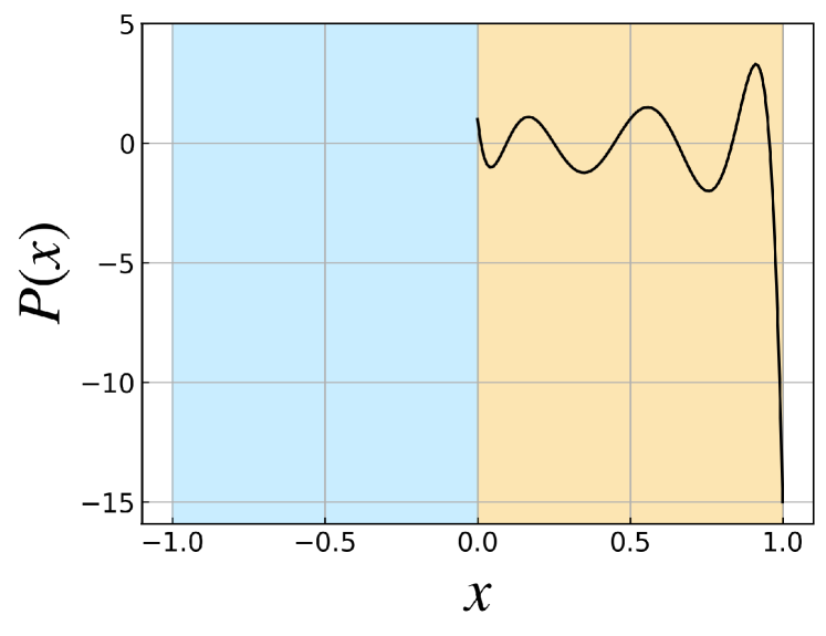
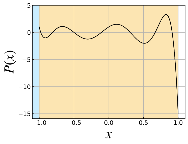
We introduce a novel technique named positive-side QET to address the issue discussed in Sec. 2.3. Let $A$ be a positive semidefinite Hermitian matrix, $U_{A}$ be a $(\alpha,n_{a},0)$ block encoding of $A$, and $P$ be a target real polynomial. The eigenvalues of $A/\alpha$ exist in the range $[0,1]$, indicating that the polynomial’s relevant domain lies on the positive side ($x\in[0,1]$). However, in the QET framework, the domain of interest is $[-1,1]$. To utilize only the positive side of $P(x)$, we eliminate the negative side ($x\in[-1,0]$) from the domain $[-1,1]$ by shifting and enlarging this polynomial. Specifically, we shift it by $-1/2$ in the $x$-direction and enlarge it by a factor of 2 in the $x$-direction. We denote the modified polynomial by

$$P^{+}(x)=P\left(\frac{x+1}{2}\right).$$ (32)

Figure 7 visually represents these operations.

If we compute phase factors from the modified polynomial and use the block encoding $U_{A}$, then we have

$$P^{+}(A/\alpha)=P\left(\frac{A/\alpha+I}{2}\right)\neq P(A/\alpha),$$ (33)

which does not match the target polynomial. Consequently, $U_{A}$ must be substituted with the $(1,n_{a},0)$ block encoding $U_{A^{\prime}}$ of

$$A^{\prime}=2A/\alpha-I.$$ (34)

This adjustment leads to the construction of the target polynomial

$$P^{+}(A^{\prime})=P\left(\frac{2A/\alpha-I+I}{2}\right)=P(A/\alpha).$$ (35)

Therefore, this technique allows us to amplify the success probability by a factor of $\max_{x\in[-1,1]}|P(x)|/\max_{x\in[0,1]}|P(x)|$ at only the additional cost of constructing $U_{A^{\prime}}$. The success probability can be improved dramatically if this ratio is large. Thus, for a positive semidefinite Hermitian matrix, a polynomial with a huge absolute value on the negative side can be handled more efficiently by using $U_{A^{\prime}}$ and $P^{+}(x)$ than by naively using $U_{A}$ and $P(x)$.

Refer to caption

(a)

Refer to caption

(b)

Figure 7: Illustration of shifting and enlarging a polynomial. The black curve represents $P_{r,k=6}(x)$ in Fig. 5. The orange region represents the positive side ($x\in[0,1]$) of the original polynomial, and the blue region represents the negative side ($x\in[-1,0]$). For clarity, we deliberately omit the negative side of the polynomial, which has a large magnitude.

We describe a procedure for constructing a degree-$d$ general polynomial by combining the positive-side QET with the method described in Sec. 2.1. First, we derive the polynomial $P^{+}(x)$ from the original polynomial $P(x)$ and divide it into even and odd polynomials. Then we normalize these polynomials using the larger maximum absolute value for $x\in[0,1]$ instead of $x\in[-1,1]$, denoted by $C_{\max,d}$, and compute the corresponding phase factors. Finally, we construct a circuit depicted in Fig. 3 using these phase factors and $d$ queries to $U_{A^{\prime}}$. This circuit represents $(2C_{\max,d},n_{a}+2,0)$ block encoding of $P(A/\alpha)$.

Note that the above technique requires efficiently implementing the block encoding $U_{A^{\prime}}$ of $A^{\prime}$. Importantly, if $A$ is sparse, then $A^{\prime}$ is also sparse. Therefore, we can efficiently create the block encoding of $A^{\prime}$ for a sparse matrix $A$. The details of this construction remain a challenging task; however, some proposed methods exist. For instance, Refs. [41, 42] discuss schemes for building explicit circuits for block encodings of structured sparse matrices.

Additionally, we propose explicit circuits for $U_{A^{\prime}}$ from $U_{A}$, as detailed in Appendix A. We present two methods with and without a gap $\Lambda\in(0,\frac{\alpha}{2})$. This gap is related to the $A$’s eigenvalues $\{\lambda_{j}\}$ such that

$$\Lambda\leq\lambda_{j}\leq\alpha-\Lambda.$$ (36)

The method with $\Lambda$ requires $O(\frac{\alpha}{\Lambda}\log(1/\varepsilon))$ additional queries to $U_{A}$, while the method without it demands $O(\frac{1}{\varepsilon}\log(1/\varepsilon))$ additional queries. Both methods involve the linear combination of unitaries and linear amplification [8, 10, 28]. The method selection should be appropriate based on the magnitude of $\Lambda$, $\alpha$, and $\varepsilon$.

3.2 Quantum conjugate gradient method using the quantum eigenvalue transformation

Refer to caption
Figure 8: Illustration of the quantum conjugate gradient method using the quantum eigenvalue transformation.

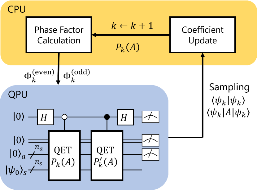
The QCG method using the QET is a hybrid quantum-classical algorithm. Quantum computations include polynomial implementations through the QET and evaluations of inner products using the swap test described in Sec. 2.4. Classical computations cover updating coefficients according to Eq. (27) and calculating the phase factors based on the updated coefficients. Figure 8 illustrates the QCG method using the QET.

{algorithm*}

[t] Quantum conjugate gradient method using the quantum eigenvalue transformation.

0:  
1:  $\ket{x_{0}}=0,\ket{r_{0}}=\ket{p_{0}}=\frac{\ket{b}}{\|\ket{b}\|}$
2:  Estimate $\braket{p_{0}}{p^{\prime}_{0}}$ using the swap test with $\delta$ precision.
3:  for $k=0,1,\ldots,m$ do
4:     $\alpha_{k}=\frac{\braket{r_{k}}{r_{k}}}{\braket{p_{k}}{p^{\prime}_{k}}}$
5:     for $l=0,1,\ldots,k,k+1$ do
6:        $x_{k+1,l}=x_{k,l}+\alpha_{k}p_{k,l}$
7:        $r_{k+1,l}=r_{k,l}-\alpha_{k}p_{k,l-1}$
8:     end for
9:     Compute $R_{\max,k+1}$ from $\{r_{k+1,l}\}$ and the phase factors for the normalized even and odd polynomials.
10:     Estimate $\frac{\braket{r_{k+1}}{r_{k+1}}}{4R_{\max,k+1}^{2}}$ using the swap test with $\frac{\delta}{4R_{\max,k+1}^{2}}$ precision.
11:     if $\left\|\ket{r_{k+1}}\right\|\leq\frac{\|A\|\varepsilon}{\kappa\|\ket{b}\|}$ then
12:        BREAK
13:     end if
14:     $\beta_{k}=\frac{\braket{r_{k+1}}{r_{k+1}}}{\braket{r_{k}}{r_{k}}}$
15:     for $l=0,1,\ldots,k,k+1$ do
16:        $p_{k+1,l}=r_{k+1,l}+\beta_{k}p_{k,l}$
17:     end for
18:     Compute $P_{\max,k+1}$ and $P^{\prime}_{\max,k+1}$ from $\{p_{k+1,l}\}$ and the phase factors for the normalized even and odd polynomials.
19:     Estimate $\frac{\braket{p_{k+1}}{p^{\prime}_{k+1}}}{4P_{\max,k+1}P^{\prime}_{\max,k+1}}$ using the swap test with $\frac{\delta}{4P_{\max,k+1}P^{\prime}_{\max,k+1}}$ precision.
20:  end for
21:  Compute $X_{\max,m+1}$ from $\{x_{m+1,l}\}$ and the phase factors for the normalized even and odd polynomials.
22:  Prepare the state proportional to $\frac{1}{2X_{\max,m+1}}\ket{x_{m+1}}$.

We introduce some notations to elaborate on the QCG method in detail. Although our goal is to solve $A\ket{x}=\ket{b}$, the $(\alpha,n_{a},0)$ block encoding of $A$ and the initial vector $\frac{\ket{b}}{\|\ket{b}\|}$ are applied to the QCG method. Consequently, the vectors are represented as

$\displaystyle\begin{split}\ket{x_{k}}&=P_{x,k}\left(\frac{A}{\alpha}\right)\frac{\ket{b}}{\|\ket{b}\|}=\sum_{l=0}^{k-1}x_{k,l}\left(\frac{A}{\alpha}\right)^{l}\frac{\ket{b}}{\|\ket{b}\|},\\ \ket{r_{k}}&=P_{r,k}\left(\frac{A}{\alpha}\right)\frac{\ket{b}}{\|\ket{b}\|}=\sum_{l=0}^{k}r_{k,l}\left(\frac{A}{\alpha}\right)^{l}\frac{\ket{b}}{\|\ket{b}\|},\\ \ket{p_{k}}&=P_{p,k}\left(\frac{A}{\alpha}\right)\frac{\ket{b}}{\|\ket{b}\|}=\sum_{l=0}^{k}p_{k,l}\left(\frac{A}{\alpha}\right)^{l}\frac{\ket{b}}{\|\ket{b}\|},\\ \ket{p^{\prime}_{k}}&=\frac{A}{\alpha}\ket{p_{k}}=\frac{A}{\alpha}P_{p,k}\left(\frac{A}{\alpha}\right)\frac{\ket{b}}{\|\ket{b}\|}.\end{split}$ (37)

The approximate solution vector $\ket{x_{k}}$ approximates $\frac{\alpha}{\|\ket{b}\|}\ket{x}$, and the residual vector is expressed as $\ket{r_{k}}=\frac{\ket{b}}{\|\ket{b}\|}-\frac{A}{\alpha}\ket{x_{k}}$. The corresponding absolute maximum values of the above polynomials for $x\in[0,1]$ are denoted by $X_{\max,k},R_{\max,k},P_{\max,k}$, and $P^{\prime}_{\max,k}$. The accuracy of inner product estimations is $\delta>0$. Algorithm 8 summarizes the QCG method using the QET.

In classical computing, the convergence of the CG method has been extensively examined [2, 3]. This result is applied to the QCG method, and the convergence is expressed through the inequality

$\displaystyle\left\|\frac{\alpha}{\|\ket{b}\|}\ket{x}-\ket{x_{k}}\right\|_{\frac{A}{\alpha}}$
$\displaystyle\leq 2\left(\frac{\sqrt{\kappa}-1}{\sqrt{\kappa}+1}\right)^{k}\left\|\frac{\alpha}{\|\ket{b}\|}\ket{x}-\ket{x_{0}}\right\|_{\frac{A}{\alpha}}$ (38)

where $\|\cdot\|_{A}$ represents the $A$-norm such that $\|\ket{\psi}\|_{A}=\sqrt{\bra{\psi}A\ket{\psi}}$. Since $\ket{x_{0}}=0$ and $\|\ket{x}\|_{\frac{A}{\alpha}}=\|\sqrt{\frac{A}{\alpha}}\ket{x}\|\leq\|\ket{x}\|\leq\frac{\kappa\|\ket{b}\|}{\|A\|}$, we have

$$\left\|\ket{x}-\frac{\|\ket{b}\|}{\alpha}\ket{x_{k}}\right\|_{\frac{A}{\alpha}}\leq 2\left(\frac{\sqrt{\kappa}-1}{\sqrt{\kappa}+1}\right)^{k}\frac{\kappa\|\ket{b}\|}{\|A\|}.$$ (39)

A sufficient number of iterations are executed to decrease the above norm by a factor of $\varepsilon>0$; that is, $\left\|\ket{x}-\frac{\|\ket{b}\|}{\alpha}\ket{x_{k}}\right\|_{\frac{A}{\alpha}}\leq\varepsilon$. As a result, the maximum number of iterations is given by

$\displaystyle k$ $\displaystyle=\left\lceil\frac{1}{2}\sqrt{\kappa}\ln\left(\frac{2\kappa\|\ket{b}\|}{\|A\|\varepsilon}\right)\right\rceil$
$\displaystyle=O\left(\sqrt{\kappa}\log\left(\frac{\kappa\|\ket{b}\|}{\|A\|\varepsilon}\right)\right).$ (40)

However, since the solution $\ket{x}$ is unknown, we cannot access $\left\|\ket{x}-\frac{\|\ket{b}\|}{\alpha}\ket{x_{k}}\right\|_{\frac{A}{\alpha}}$. Instead, we use the residual $\|\ket{r_{k}}\|$. If the inequality $\|\ket{r_{k}}\|\leq\frac{\|A\|\varepsilon}{\kappa\|\ket{b}\|}$ holds, then the following inequalities also hold:

$\displaystyle\left\|\ket{x}-\frac{\|\ket{b}\|}{\alpha}\ket{x_{k}}\right\|$ $\displaystyle=\left\|A^{-1}\ket{b}-\frac{\|\ket{b}\|}{\alpha}A^{-1}A\ket{x_{k}}\right\|$
$\displaystyle\leq\|A^{-1}\|\|\ket{b}\|\|\ket{r_{k}}\|$
$\displaystyle\leq\|A^{-1}\|\|\ket{b}\|\cdot\frac{\|A\|\varepsilon}{\kappa\|\ket{b}\|}=\varepsilon,$ (41)

and

$\displaystyle\left\|\ket{x}-\frac{\|\ket{b}\|}{\alpha}\ket{x_{k}}\right\|_{\frac{A}{\alpha}}$ $\displaystyle=\left\|\sqrt{\frac{A}{\alpha}}\left(\ket{x}-\frac{\|\ket{b}\|}{\alpha}\ket{x_{k}}\right)\right\|$
$\displaystyle\leq\left\|\sqrt{\frac{A}{\alpha}}\right\|\left\|\ket{x}-\frac{\|\ket{b}\|}{\alpha}\ket{x_{k}}\right\|$
$\displaystyle\leq\varepsilon.$ (42)

If we define $\|\ket{r_{k}}\|\leq\frac{\|A\|\varepsilon}{\kappa\|\ket{b}\|}$ as a convergence criterion, the algorithm stops after the number of iterations in Eq. (3.2).

In practical application, the computation does not precisely converge in the above number of iterations due to estimate errors from swap tests. Therefore, we need sufficiently accurate estimations. According to the convergence criterion, the inequality $\braket{r_{k}}{r_{k}}\leq\left(\frac{\|A\|\varepsilon}{\kappa\|\ket{b}\|}\right)^{2}$ holds; thus, we require $\delta<\left(\frac{\|A\|\varepsilon}{\kappa\|\ket{b}\|}\right)^{2}$.

Under this assumption, the computation of the QCG method using the QET can also stop after $m=O\left(\sqrt{\kappa}\log\left(\frac{\kappa\|\ket{b}\|}{\|A\|\varepsilon}\right)\right)$ iterations. Since the circuit for estimating $\braket{r_{m+1}}{r_{m+1}}$ exhibits the highest depth in Algorithm 8, the maximum circuit depth is

$$2(m+1)=O\left(\sqrt{\kappa}\log\left(\frac{\kappa\|\ket{b}\|}{\|A\|\varepsilon}\right)\right).$$ (43)

This outcome indicates that this algorithm improves the maximum circuit depth compared to other QLSAs [4, 5, 6, 7, 8, 9, 10].

Here we discuss the total query complexity of the QCG method using the QET. In the $k$ th iteration, the total number of queries to the block encoding scales as

$\displaystyle\begin{split}Q_{k}\equiv O\Bigg{(}&\frac{32(k+1)R_{\max,k+1}^{4}}{\delta^{2}}\\ &\quad+\frac{16(2k+3)P_{\max,k+1}^{2}P_{\max,k+1}^{{}^{\prime}2}}{\delta^{2}}\Bigg{)}.\end{split}$ (44)

Generating $\frac{1}{2X_{\max,m+1}}\ket{x_{m+1}}$ requires $m$ queries, and obtaining the state $\frac{\ket{x_{m+1}}}{\|\ket{x_{m+1}}\|}$ demands $O\left(\frac{2X_{\max,m+1}^{2}}{\|\ket{x_{m+1}}\|^{2}}\right)$ circuit runs. Therefore, the total query complexity is expressed as

$$O\left(\sum_{k=0}^{m}Q_{k}+m\left(\frac{2X_{\max,m+1}}{\|\ket{x_{m+1}}\|}\right)^{2}\right).$$ (45)

For simplicity, we assume that the maximum absolute values of the polynomials depend on the iteration number $k$ as follows:

$\displaystyle\begin{split}X_{\max,k}&=O(k^{\gamma_{x}}),\quad R_{\max,k}=O(k^{\gamma_{r}}),\\ P_{\max,k}&=O(k^{\gamma_{p}}),\quad P^{\prime}_{\max,k}=O(k^{\gamma_{p^{\prime}}}),\end{split}$ (46)

where $\gamma_{r},\gamma_{p},\gamma_{p^{\prime}},\gamma_{x}\geq 0$. Consequently, Eq. (45) scales as

$\displaystyle O\left(\sum_{k=0}^{m+1}\frac{k(k^{4\gamma_{r}}+k^{2(\gamma_{p}+\gamma_{p^{\prime}})})}{\delta^{2}}+\frac{m^{1+2\gamma_{x}}}{\|\ket{x_{m+1}}\|^{2}}\right)$
$\displaystyle=O\left(\frac{m^{2}(m^{4\gamma_{r}}+m^{2(\gamma_{p}+\gamma_{p^{\prime}})})}{\delta^{2}}+\frac{m^{1+2\gamma_{x}}}{\|\ket{x_{m+1}}\|^{2}}\right)$
$\displaystyle=O\left(\left[\frac{\kappa^{1+\gamma}}{\delta^{2}}+\frac{\kappa^{\frac{1}{2}+\gamma_{x}}}{\|\ket{x_{m+1}}\|^{2}}\right]\mathrm{polylog}\left(\frac{\kappa\|\ket{b}\|}{\|A\|\varepsilon}\right)\right),$ (47)

where in the last equality, we used $\gamma\equiv\max\{2\gamma_{r},\gamma_{p}+\gamma_{p^{\prime}}\}$ and $m=O\left(\sqrt{\kappa}\log\left(\frac{\kappa\|\ket{b}\|}{\|A\|\varepsilon}\right)\right)$. Additionally, we assume that the estimation accuracy is such that $c\left(\frac{\|A\|\varepsilon}{\kappa\|\ket{b}\|}\right)^{2}<\delta<\left(\frac{\|A\|\varepsilon}{\kappa\|\ket{b}\|}\right)^{2}$ for a constant $c\in(0,1)$. The approximate solution is assumed to satisfy $\|\ket{x_{k}}\|=\Omega(1)$ as a worst-case. Equation (47) becomes

$$O\left(\left[\kappa^{5+\gamma}\left(\frac{\|\ket{b}\|}{\|A\|\varepsilon}\right)^{4}+\kappa^{\frac{1}{2}+\gamma_{x}}\right]\mathrm{polylog}\left(\frac{\kappa\|\ket{b}\|}{\|A\|\varepsilon}\right)\right).$$ (48)

Note that this scaling does not include the subnormalization factor $\alpha$. This absence occurs when the block encoding of $A^{\prime}=2\frac{A}{\alpha}-I$ is present or is constructed using the method without the gap of Appendix A. However, if the method with the gap is utilized, the total query complexity depends on $\alpha$.

The validity of the assumption in Eq. (46) varies; it holds in some cases but not in others, as demonstrated by the numerical experiments in Sec. 4. In a particular simulation, the maximum absolute values depend on $\kappa$ instead of $k$ as follows:

$\displaystyle\begin{split}X_{\max,k}&=O(\kappa^{\eta_{x}}),\quad R_{\max,k}=O(\kappa^{\eta_{r}}),\\ P_{\max,k}&=O(\kappa^{\eta_{p}}),\quad P^{\prime}_{\max,k}=O(\kappa^{\eta_{p^{\prime}}}),\end{split}$ (49)

where $\eta_{r},\eta_{p},\eta_{p^{\prime}},\eta_{x}\geq 0$. Accordingly, the total query complexity scales as

$$O\left(\left[\kappa^{5+\eta}\left(\frac{\|\ket{b}\|}{\|A\|\varepsilon}\right)^{4}+\kappa^{\frac{1}{2}+2\eta_{x}}\right]\mathrm{polylog}\left(\frac{\kappa\|\ket{b}\|}{\|A\|\varepsilon}\right)\right),$$ (50)

where $\eta\equiv\max\{4\eta_{r},2(\eta_{p}+\eta_{p^{\prime}})\}$.

In either case, the scaling for $\kappa$ and $\varepsilon$ is less favorable than that of the other QLSAs [4, 5, 6, 7, 8, 9, 10]. This scaling results from numerous circuit runs to attain precise estimates of inner products through the swap tests. Our algorithm can be interpreted as prioritizing a low circuit depth at the expense of an increased number of circuit runs.

It is essential to highlight that the total query complexity is worst-case because the precision required to estimate all inner products must be less than $\left(\frac{\|A\|\varepsilon}{\kappa\|\ket{b}\|}\right)^{2}$. This precision is chosen to estimate the residual. However, as seen in the numerical results of Sec. 4, the residuals are not small unless the algorithm stops, meeting the convergence criterion. If high precision is unnecessary in the early stages of iterations, the number of circuit runs can be reduced. Moreover, quantum amplitude estimation [38, 39, 40] can be applied within an acceptable circuit depth range. These considerations suggest that optimizing the number of circuit runs and the circuit depth while ensuring the algorithm’s robustness improves the total query complexity.

In summary, our algorithm achieves a square root improvement for $\kappa$ concerning the maximum circuit depth, and the number of ancilla qubits is $n_{a}+3$, regardless of both $\kappa$ and $\varepsilon$. Therefore, our algorithm fulfills shallow circuits with constant ancilla qubits. As a trade-off for the shallow circuits, the total query complexity is worse than that of other QLSAs. However, this can be improved by controlling the number of circuit runs and using the quantum amplitude estimation.

4 Numerical results

Refer to caption
Figure 9: Circuit for $(1,2,0)$ block encoding of $A^{\prime}=2\frac{A}{4}-I$. The $+1$ and $-1$ gates are defined in Fig. 10.
Refer to caption
Figure 10: Gates that change the state by $\pm 1$. The circuit (a) represents the $+1$ gate for $n$ qubits. For $j=0,1,\dots,2^{n}-1$, this gate acts as $\ket{j}_{s}\rightarrow\ket{j+1}_{s}$, where $\ket{2^{n}}_{s}\equiv\ket{0}_{s}$. The circuit (b) represents the $-1$ gate for $n$ qubits. For $j=0,1,\dots,2^{n}-1$, this gate acts as $\ket{j}_{s}\rightarrow\ket{j-1}_{s}$, where $\ket{-1}_{s}\equiv\ket{2^{n}-1}_{s}$.
Refer to caption
Figure 11: Plots of the residuals obtained in the simulations ($N=16$).

We conduct numerical experiments on the Poisson equation to validate the QCG method using the QET. The one-dimensional Poisson equation is represented as

$$\frac{d^{2}\phi}{dr^{2}}=-\rho(r),$$ (51)

where $\rho$ is a given function, and $\phi$ is an unknown function. We discretize the above equation using the second-order central difference scheme with the Dirichlet boundary conditions $\rho(r_{L})=\rho(r_{R})=0$. This results in a linear system of equations $A\ket{x}=\ket{b}$ for

$$A=\begin{bmatrix}2&-1&0&\cdots&0\\ -1&2&-1&\cdots&0\\ 0&-1&\ddots&\ddots&\vdots\\ \vdots&\vdots&\ddots&2&-1\\ 0&\cdots&0&-1&2\end{bmatrix},$$ (52)
$\displaystyle\ket{x}$ $\displaystyle=\left[\phi_{0},\phi_{1},\cdots,\phi_{N-1}\right]^{\top},$ (53)
$\displaystyle\ket{b}$ $\displaystyle=\left[\rho_{0}(\Delta x)^{2},\rho_{1}(\Delta x)^{2},\cdots,\rho_{N-1}(\Delta x)^{2}\right]^{\top},$ (54)

where $N$ is the system size and $\Delta x=\frac{r_{R}-r_{L}}{N+1}$. Since the matrix $A$ is a positive definite Hermitian matrix, the QCG method can solve this system. Figure 10 shows the circuit for $(1,2,0)$ block encoding of $A^{\prime}=2\frac{A}{4}-I$ ($\alpha=4$). The $+1$ and $-1$ gates in this circuit are presented in Fig. 10. It is important to note that the subnormalization factor must satisfy $\alpha\geq 4$ because the maximum eigenvalue of $A$ is nearly $4$. Therefore, the block encoding described above is nearly optimal in terms of the subnormalization factor.

We consider the system size $N=16$ and two cases for the initial vectors

$\displaystyle\mathrm{Case}\ 1:$ $\displaystyle\quad\ket{b}=\frac{1}{\sqrt{2}}(\ket{N/2-1}+\ket{N/2}),$
$\displaystyle\mathrm{Case}\ 2:$ $\displaystyle\quad\ket{b}=\frac{1}{\sqrt{N}}\sum_{j=0}^{N-1}\ket{j},$

which can be efficiently prepared using the Hadamard gates. Based on classical numerical calculations, the condition number is $\kappa\approx 116$, and the norm is $\|A\|\approx 3.97$. The error tolerance is $\varepsilon=0.1$, and the convergence criterion is $\||\ket{r_{k}}\|\leq\|A\|\varepsilon/\kappa\|\ket{b}\|=3.40\times 10^{-3}$. States and their inner products are computed using Statevector Simulator of Qiskt [18] as a backend. The QSPPACK [32, 33, 35, 43] is used to calculate phase factors.

Table 1: Comparison of polynomial degrees between the QCG method using the QET and the QLSA using the direct QSVT [10] for the one-dimensional Poisson equation. Both cases have the same number of iterations. Note that the condition number scales as $\kappa=O(N^{2})$ for the system size $N$.
System size Condition number Polynomial degree
$N$ $\kappa$ QCG Direct QSVT Rectangular function
4 9.47 2 $7.45\times 10^{3}$ $6.61\times 10^{3}$
8 32.2 4 $2.88\times 10^{4}$ $2.55\times 10^{4}$
16 116 8 $1.18\times 10^{5}$ $1.05\times 10^{5}$
32 441 16 $5.05\times 10^{5}$ $4.45\times 10^{5}$
Refer to caption

(a)

Refer to caption

(b)

Figure 12: Plots of the maximum absolute values of polynomials for $x\in[0,1]$ ($N=16$): (a) For Case 1 and (b) for Case 2. The curve and straight lines in (a) represent the results of fitting quadratic and linear functions. The gray dashed line in (b) represents the condition number $\kappa\approx 116$.

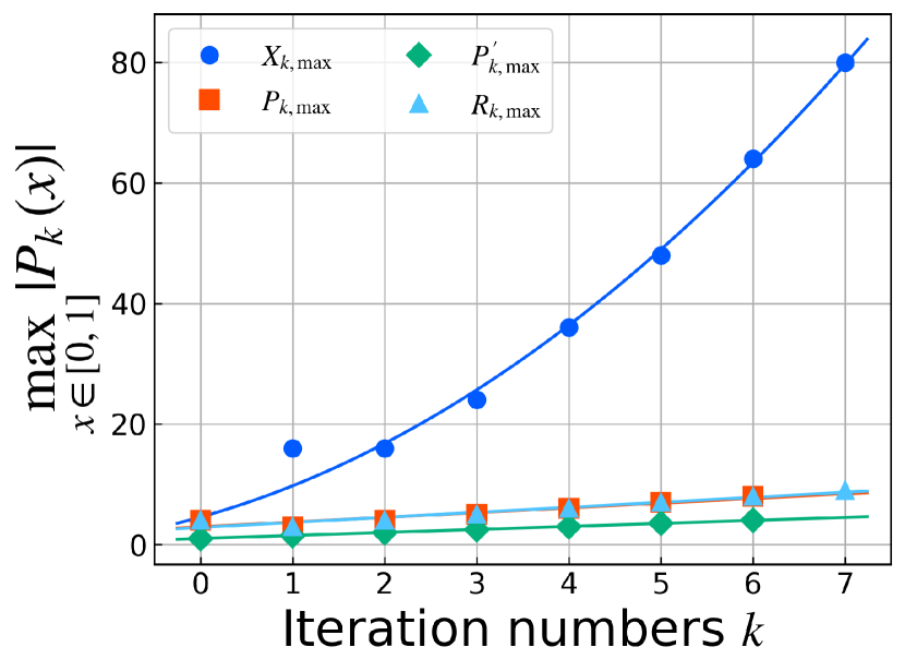
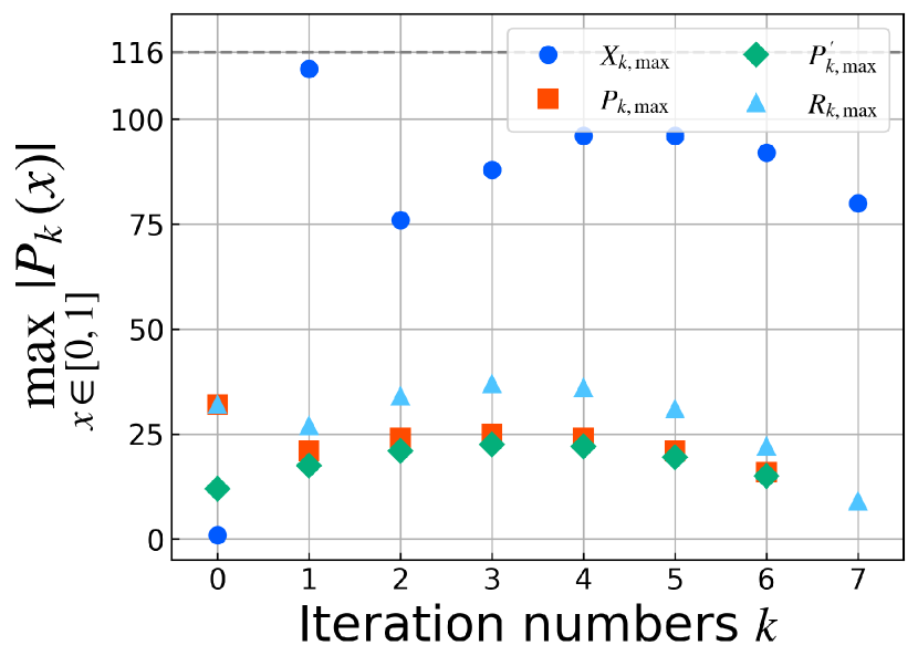
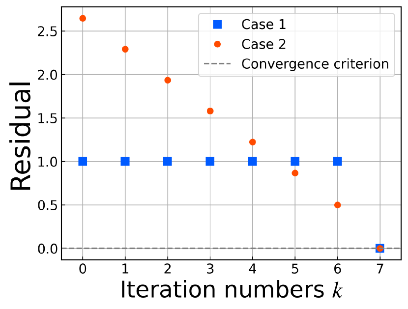
Figure 11 shows the plots of the residuals. As iterations progress, the residuals decrease, and the algorithm converges, meeting the convergence criterion at the seventh iteration. At this point, the residual and error are shown below: For Case 1,

$\displaystyle\begin{split}\|\ket{r_{8}}\|&=1.89\times 10^{-5}<3.40\times 10^{-3},\\ \left\|\ket{x}-\frac{1}{\alpha}\ket{x_{8}}\right\|&=8.71\times 10^{-5}<0.1,\end{split}$

and for Case 2,

$\displaystyle\begin{split}\|\ket{r_{8}}\|&=2.84\times 10^{-5}<3.40\times 10^{-3},\\ \left\|\ket{x}-\frac{1}{\alpha}\ket{x_{8}}\right\|&=2.71\times 10^{-4}<0.1.\end{split}$

These results demonstrate the successful resolution of the one-dimensional Poisson equation by our algorithm.

We compare the polynomial degrees between our algorithm and the QLSA using the direct QSVT [10] applied to the one-dimensional Poisson equation. Our algorithm determines the polynomial degree based on the number of iterations when the algorithm stops for $\varepsilon=10^{-1}$. For that number denoted by $m$, the maximum circuit depth is represented as $2(m+1)$. On the other hand, in the QLSA using the direct QSVT, the polynomial degree (equivalent to the maximum circuit depth) is computed based on Eq. (25) for $\alpha=4$ and $\varepsilon=10^{-1}$.

Table 1 compares the degrees of these polynomials. Notably, this result shows a substantial reduction in the polynomial degree (the maximum circuit depth) by our algorithm compared to the direct QSVT by three to four orders of magnitude. The table also reveals that the polynomial degree of the direct QSVT is greatly influenced by the degree of the polynomial approximating the rectangular function, which consists of the sign function. This finding indicates that approximating the sign function demands high polynomial degree.

Figure 12 plots the maximum absolute values of polynomials for $x\in[0,1]$ ($N=16$). The scalings of these values for Case 1 are

$$X_{k,\max}=O(k^{2}),\quad P_{k,\max},P^{\prime}_{k,\max},R_{k,\max}=O(k).$$ (55)

On the other hand, the values for Case 2 depend on $\kappa$ rather than $k$. Numerous circuit runs are required for both cases, as seen in the scaling of Eq. (45) or (47) because these values are not close to 1. Therefore, in the problem setting of the Poisson equation, the total query complexity is enormous, although the circuit depth remains shallow.

5 Discussion

In the QLSAs, the parameters $N$ and $\kappa$ significantly impact achieving advantages over the classical counterparts. Achieving these advantages requires $N$ to be significant and $\kappa$ to be small, especially when $\kappa$ scales as $O(\mathrm{polylog}(N))$. Our algorithm must also consider the dependence regarding the maximum absolute values of the polynomials. Specifically, minimizing their dependence on $k$ or $\kappa$ is essential for reducing the number of circuit runs. As shown in Fig. 12, this dependence relies on the initial vector. Inherently, it can also depend on the given matrix $A$. Investigating the dependence concerning $A$ and $\ket{b}$ is a subject for future work.

The positive-side QET can be generalized when the Hermitian matrix is not positive semidefinite. Suppose that we know in advance that the eigenvalues of $A/\alpha$ exist in $[\delta_{1},\delta_{2}]$ for a Hermitian matrix $A$ and $-1\leq\delta_{1}<\delta_{2}\leq 1$. We use the polynomial and matrix

$\displaystyle P^{\mathrm{new}}(x)$ $\displaystyle=P\left(\frac{\delta_{2}-\delta_{1}}{2}x+\frac{\delta_{1}+\delta_{2}}{2}\right),$ (56)
$\displaystyle A^{\prime}$ $\displaystyle=\frac{2}{\delta_{2}-\delta_{1}}\frac{A}{\alpha}-\frac{\delta_{1}+\delta_{2}}{\delta_{2}-\delta_{1}}I.$ (57)

Consequently, we eliminate the unnecessary region ($x\in[-1,\delta_{1}]\cup[\delta_{2},1]$) of the original polynomial from the range $[-1,1]$. As discussed in Sec. 3.1, we can efficiently construct the block encoding of $A^{\prime}$ for a sparse matrix $A$. Moreover, one can approximately build the block encoding of $A^{\prime}$ from that of $A$ using the same procedure described in Appendix A.

Although the circuit depth scaling of the QLSA using direct QSVT is nearly optimal, the constant factor is significant. This is attributed to the high degree of the polynomial used to approximate the sign function. This observation suggests that algorithms based on QSVT using approximate polynomials of the sign function might face this issue. Additionally, calculating phase factors for polynomials with a high degree ($10^{5}\sim$) seems challenging [30, 31, 32, 33, 34, 35]. Therefore, reducing the polynomial degree is necessary for both the circuit depth and phase factor calculations.

The CG method works well for only positive definite Hermitian matrices. However, if we define $B=AA^{\dagger}$ for a general matrix $A$, then $B$ becomes positive semidefinite and Hermitian. Accordingly, the solution takes the form $\ket{x}=A^{\dagger}B^{-1}\ket{b}$, enabling the resolution of linear systems of equations for general matrices through the QCG method using the QET. However, the condition number of $B$ becomes $\kappa^{2}$, where $\kappa$ is the condition number of $A$. As a result, the maximum circuit depth shows a linear dependence on $\kappa$. This increase diminishes the advantage of the QCG method in terms of circuit depth.

The CG method is a form of the Krylov subspace method, which is used for solving linear systems of equations and eigenvalue problems [2, 3]. In particular, the Lanczos method is designed to create a Krylov subspace for Hermitian matrices. The vectors obtained through this method can also be represented as the product of a polynomial $P(A)$ and an initial vector $\ket{b}$ (as discussed in  [7]). Therefore, the Lanczos method can be implemented using the QET. Similarly, considering $B=AA^{\dagger}$ for a general matrix $A$ allows the implementation of the Krylov subspace method in the QET framework.

6 Summary

This paper introduces the quantum conjugate gradient method using the quantum eigenvalue transformation. Additionally, we propose a new technique called the positive-side QET. This technique enables the implementation of polynomials with huge absolute values on the negative side ($x\in[-1,0]$), which cannot be handled in the previous QET framework. The QCG method using the positive-side QET achieves a maximum circuit depth of $O\left(\sqrt{\kappa}\log\left(\frac{\kappa\|\ket{b}\|}{\|A\|\varepsilon}\right)\right)$. This scaling represents a square root improvement for $\kappa$ compared to earlier QLSAs [4, 5, 6, 7, 8, 9, 10]. Moreover, the number of ancilla qubits remains constant. Therefore, our algorithm accomplishes shallow circuits with minimal ancilla qubits. However, the algorithm demands numerous circuit runs, resulting in an unfavorable total query complexity. To mitigate this cost, one can optimize a tradeoff between the precision for estimating inner products and the number of circuit runs, a topic for future investigation.

Acknowledgements

This work was supported by MEXT Quantum Leap Flagship Program Grants No. JPMXS0118067285 and No. JPMXS0120319794. K.W. was supported by JST SPRING, Grant No. JPMJSP2123.

Appendix A Explicit circuits for the block encoding of $A^{\prime}$

We discuss the explicit circuits constructing the block encoding of $A^{\prime}=2A/\alpha-I$ from the block encoding of $A$. Let $A$ be a Hermitian matrix and $U_{A}$ be a $(\alpha,n_{a},0)$ block encoding of $A$. First, we construct the block encoding of the matrix $\frac{1}{\gamma}A^{\prime}$ using linear combination of unitaries, where $\gamma>1$ is an amplification factor. Figure 13 shows the circuit $U^{\prime}_{A^{\prime}}$ for the $(3,n_{a}+1,0)$ block encoding of $A^{\prime}$.

Since $1/\gamma=1/3$ is unnecessary, this factor must be amplified to $1$. This amplification can be achieved by linear amplification [28, 8, 10], also called uniform spectral amplification. Importantly, this method can be implemented using the QET (QSVT). The polynomial for the linear amplification is represented as the product of $\gamma x$ and the approximate polynomial of the closed rectangular mentioned in Sec. 2.1.1. We present two methods for the linear amplification: One involving a gap $\Lambda$ related to the eigenvalues of $A$ and an alternative method without the gap.

Refer to caption
Figure 13: The circuit $U^{\prime}_{A^{\prime}}$ for the $(3,n_{a}+1,0)$ block encoding of $A^{\prime}=2\frac{A}{\alpha}-I$. The angle is $\theta=2\tan^{-1}\sqrt{\frac{1}{2}}$.

A.1 Method with the gap $\Lambda$

Let $\{\lambda_{j}\}$ be the eigenvalues of $A$ and $\Lambda\in(0,\frac{\alpha}{2})$ be a gap such that

$$\Lambda\leq\lambda_{j}\leq\alpha-\Lambda.$$ (A1 )

Therefore, we have

$$-\frac{1-2\Lambda^{\prime}}{\gamma}\leq\frac{2\frac{\lambda_{j}}{\alpha}-1}{\gamma}\leq\frac{1-2\Lambda^{\prime}}{\gamma},$$ (A2 )

where $\Lambda^{\prime}=\frac{\Lambda}{\alpha}$. For $\gamma>1$, one choice of the approximate polynomial for the closed rectangular function is represented as $P_{\frac{1-\Lambda^{\prime}}{\gamma},\frac{2\Lambda^{\prime}}{\gamma},\frac{\varepsilon}{\gamma}}^{\mathrm{rect}}(x)$ such that

$\displaystyle\begin{split}\left|1-P_{\frac{1-\Lambda^{\prime}}{\gamma},\frac{2\Lambda^{\prime}}{\gamma},\frac{\varepsilon}{\gamma}}^{\mathrm{rect}}(x)\right|&\leq\frac{\varepsilon}{\gamma},\\ &x\in\left[-\frac{1-2\Lambda^{\prime}}{\gamma},\frac{1-2\Lambda^{\prime}}{\gamma}\right],\\ \left|P_{\frac{1-\Lambda^{\prime}}{\gamma},\frac{2\Lambda^{\prime}}{\gamma},\frac{\varepsilon}{\gamma}}^{\mathrm{rect}}(x)\right|&\leq\frac{\varepsilon}{\gamma},\\ &x\in\left[-1,-\frac{1}{\gamma}\right]\cup\left[\frac{1}{\gamma},1\right],\\ \left|P_{\frac{1-\Lambda^{\prime}}{\gamma},\frac{2\Lambda^{\prime}}{\gamma},\frac{\varepsilon}{\gamma}}^{\mathrm{rect}}(x)\right|&\leq 1,\quad x\in\left[-1,1\right].\end{split}$ (A3 )

Then the polynomial for the linear amplification is defined by

$$P_{\gamma,\alpha,\Lambda,\varepsilon}^{\mathrm{lamp}}(x)=\gamma xP_{\frac{1-\Lambda^{\prime}}{\gamma},\frac{2\Lambda^{\prime}}{\gamma},\frac{\varepsilon}{\gamma}}^{\mathrm{rect}}(x).$$ (A4 )

This polynomial degree is expressed as

$\displaystyle d_{\mathrm{lamp}}(\gamma,\alpha,\Lambda,\varepsilon)$ $\displaystyle=d_{\mathrm{rect}}\left(\frac{1-\Lambda^{\prime}}{\gamma},\frac{2\Lambda^{\prime}}{\gamma},\frac{\varepsilon}{\gamma}\right)+1$
$\displaystyle=\mathcal{O}\left(\frac{\gamma\alpha}{\Lambda}\log\left(\frac{\gamma}{\varepsilon}\right)\right).$ (A5 )

The polynomial $P_{\gamma,\alpha,\Lambda,\varepsilon}^{\mathrm{lamp}}(x)$ satisfies the following inequalities: For $|x|\leq\frac{1-2\Lambda^{\prime}}{\gamma}$,

$\displaystyle\left|\gamma x-P_{\gamma,\alpha,\Lambda,\varepsilon}^{\mathrm{lamp}}(x)\right|$ $\displaystyle\quad\leq\gamma|x|\left|1-P_{\frac{1-\Lambda^{\prime}}{\gamma},\frac{2\Lambda^{\prime}}{\gamma},\frac{\varepsilon}{\gamma}}^{\mathrm{rect}}(x)\right|$
$\displaystyle\quad\leq\gamma\cdot\frac{1-2\Lambda^{\prime}}{\gamma}\cdot\frac{\varepsilon}{\gamma}<\varepsilon.$

For $|x|\leq\frac{1}{\gamma}$,

$\displaystyle\left|P_{\gamma,\alpha,\Lambda^{\prime},\varepsilon}^{\mathrm{lamp}}(x)\right|$ $\displaystyle\leq\gamma|x|\left|P_{\frac{1-\Lambda^{\prime}}{\gamma},\frac{2\Lambda^{\prime}}{\gamma},\frac{\varepsilon}{\gamma}}^{\mathrm{rect}}(x)\right|$
$\displaystyle\leq\gamma\cdot\frac{1}{\gamma}=1.$ (A6 )

For $\frac{1}{\gamma}\leq|x|\leq 1$,

$\displaystyle\left|P_{\gamma,\alpha,\Lambda^{\prime},\varepsilon}^{\mathrm{lamp}}(x)\right|$ $\displaystyle\leq\gamma|x|\left|P_{\frac{1-\Lambda^{\prime}}{\gamma},\frac{2\Lambda^{\prime}}{\gamma},\frac{\varepsilon}{\gamma}}^{\mathrm{rect}}(x)\right|$
$\displaystyle\leq\gamma\cdot\frac{\varepsilon}{\gamma}=\varepsilon.$ (A7 )
Table 2: Comparison of the methods for constructing the block encoding of $A^{\prime}$.
Method With $\Lambda$ Without $\Lambda$
Approximate
polynomial
$3xP_{\frac{1-\Lambda/\alpha}{3},\frac{2\Lambda}{3\alpha},\frac{\varepsilon}{3}}^{\mathrm{rect}}(x)$ $\frac{1}{1+\varepsilon/2}3xP_{\frac{1+\varepsilon/4}{3},\frac{\varepsilon}{6},\frac{\varepsilon}{6}}^{\mathrm{rect}}(x)$
Query complexity $O\left(\frac{\alpha}{\Lambda}\log(1/\varepsilon)\right)$ $O\left(\frac{1}{\varepsilon}\log(1/\varepsilon)\right)$
Requirement
The gap $\Lambda$ is large and
the subnormalization factor $\alpha$ is small.
The precision $\varepsilon$ is not small.

We denote the spectral decomposition of a Hermitian matrix $B$ by

$$B=\sum_{j}\lambda_{j}\ket{\lambda_{j}}\bra{\lambda_{j}},$$ (A8 )

where $\{\lambda_{j}\}$ is the eigenvalues such that $|\lambda_{j}|\leq\frac{1-2\Lambda^{\prime}}{\gamma}$ and $\{\ket{\lambda_{j}}\}$ is the eigenvectors. We also denote

$$\tilde{\lambda}_{j}=P_{\gamma,\alpha,\Lambda,\varepsilon}^{\mathrm{lamp}}(\lambda_{j}),$$ (A9 )

and then the inequality

$$|\gamma\lambda_{j}-\tilde{\lambda}_{j}|\leq\varepsilon$$ (A10 )

holds. Therefore, we approximately have

$\displaystyle P_{\gamma,\alpha,\Lambda,\varepsilon}^{\mathrm{lamp}}(B)$ $\displaystyle=\sum_{j}\tilde{\lambda}_{j}\ket{\lambda_{j}}\bra{\lambda_{j}}$
$\displaystyle\approx\gamma\sum_{j}\lambda_{j}\ket{\lambda_{j}}\bra{\lambda_{j}}=\gamma B.$ (A11 )

We get the $(1,n_{a}+2,\varepsilon)$ block encoding of $A^{\prime}$ by applying the above linear amplification for $\gamma=3$ to the block encoding $U^{\prime}_{A^{\prime}}$ and using the QET circuit in Fig. 1(b). The polynomial degree used in this method is

$$d_{\mathrm{lamp}}(3,\alpha,\Lambda,\varepsilon)=O\left(\frac{\alpha}{\Lambda}\log(1/\varepsilon)\right).$$ (A12 )

Therefore, the block encoding of $A^{\prime}$ is built by using $O(\frac{\alpha}{\Lambda}\log(1/\varepsilon))$ additional queries to $U_{A}$.

A.2 Method without the gap $\Lambda$

In case the gap $\Lambda$ is not used, for $\gamma>1,\varepsilon\in(0,1)$, the approximate polynomial for the closed rectangular function is represented as $P_{\frac{1+\varepsilon/4}{\gamma},\frac{\varepsilon}{2\gamma},\frac{\varepsilon}{2\gamma}}^{\mathrm{rect}}(x)$ and satisfies the inequalities

$\displaystyle\begin{split}\Bigl{|}1-&P_{\frac{1+\varepsilon/4}{\gamma},\frac{\varepsilon}{2\gamma},\frac{\varepsilon}{2\gamma}}^{\mathrm{rect}}(x)\Bigr{|}\leq\frac{\varepsilon}{2\gamma},\quad x\in\left[-\frac{1}{\gamma},\frac{1}{\gamma}\right],\\ \Bigl{|}&P_{\frac{1+\varepsilon/4}{\gamma},\frac{\varepsilon}{2\gamma},\frac{\varepsilon}{2\gamma}}^{\mathrm{rect}}(x)\Bigr{|}\leq\frac{\varepsilon}{2\gamma},\\ &\qquad x\in\left[-1,-\frac{1+\varepsilon/2}{\gamma}\right]\cup\left[\frac{1+\varepsilon/2}{\gamma},1\right],\\ \Bigl{|}&P_{\frac{1+\varepsilon/4}{\gamma},\frac{\varepsilon}{2\gamma},\frac{\varepsilon}{2\gamma}}^{\mathrm{rect}}(x)\Bigr{|}\leq 1,\quad x\in\left[-1,1\right].\end{split}$ (A13 )

Then the polynomial for the linear amplification is defined by

$$P_{\gamma,\varepsilon}^{\mathrm{lamp}}(x)=\frac{1}{1+\varepsilon/2}\gamma xP_{\frac{1+\varepsilon/4}{\gamma},\frac{\varepsilon}{2\gamma},\frac{\varepsilon}{2\gamma}}^{\mathrm{rect}}(x).$$ (A14 )

This polynomial degree is expressed as

$\displaystyle d_{\mathrm{lamp}}(\gamma,\varepsilon)$ $\displaystyle=d_{\mathrm{rect}}\left(\frac{1+\varepsilon/4}{\gamma},\frac{\varepsilon}{2\gamma},\frac{\varepsilon}{2\gamma}\right)+1$
$\displaystyle=O\left(\frac{\gamma}{\varepsilon}\log\left(\frac{\gamma}{\varepsilon}\right)\right).$ (A15 )

The polynomial $P_{\gamma,\varepsilon}^{\mathrm{lamp}}(x)$ satisfies the following inequalities: For $|x|\leq\frac{1}{\gamma}$,

$\displaystyle\left|\gamma x-P_{\gamma,\varepsilon}^{\mathrm{lamp}}(x)\right|$
$\displaystyle\leq\gamma|x|\left|1-\frac{1}{1+\varepsilon/2}P_{\frac{1+\varepsilon/4}{\gamma},\frac{\varepsilon}{2\gamma},\frac{\varepsilon}{2\gamma}}^{\mathrm{rect}}(x)\right|$
$\displaystyle\leq\gamma\cdot\frac{1}{\gamma}\left(\frac{1}{1+\varepsilon/2}\left|1-P_{\frac{1+\varepsilon/4}{\gamma},\frac{\varepsilon}{2\gamma},\frac{\varepsilon}{2\gamma}}^{\mathrm{rect}}(x)\right|+\frac{\varepsilon/2}{1+\varepsilon/2}\right)$
$\displaystyle\leq\frac{\varepsilon/2\gamma}{1+\varepsilon/2}+\frac{\varepsilon/2}{1+\varepsilon/2}<\varepsilon,$ (A16 )

and

$\displaystyle\left|P_{\gamma,\varepsilon}^{\mathrm{lamp}}(x)\right|$ $\displaystyle\leq\frac{1}{1+\varepsilon/2}\gamma|x|\left|P_{\frac{1+\varepsilon/4}{\gamma},\frac{\varepsilon}{2\gamma},\frac{\varepsilon}{2\gamma}}^{\mathrm{rect}}(x)\right|$
$\displaystyle\leq\frac{1}{1+\varepsilon/2}\gamma\cdot\frac{1}{\gamma}<1.$ (A17 )

For $\frac{1}{\gamma}\leq|x|\leq\frac{1+\varepsilon/2}{\gamma}$,

$\displaystyle\left|P_{\gamma,\varepsilon}^{\mathrm{lamp}}(x)\right|$ $\displaystyle\leq\frac{1}{1+\varepsilon/2}\gamma|x|\left|P_{\frac{1+\varepsilon/4}{\gamma},\frac{\varepsilon}{2\gamma},\frac{\varepsilon}{2\gamma}}^{\mathrm{rect}}(x)\right|$
$\displaystyle\leq\frac{1}{1+\varepsilon/2}\gamma\cdot\frac{1+\varepsilon/2}{\gamma}=1.$ (A18 )

For $\frac{1+\varepsilon/2}{\gamma}\leq|x|\leq 1$,

$\displaystyle\left|P_{\gamma,\varepsilon}^{\mathrm{lamp}}(x)\right|$ $\displaystyle\leq\frac{1}{1+\varepsilon/2}\gamma|x|\left|P_{\frac{1+\varepsilon/4}{\gamma},\frac{\varepsilon}{2\gamma},\frac{\varepsilon}{2\gamma}}^{\mathrm{rect}}(x)\right|$
$\displaystyle\leq\frac{1}{1+\varepsilon/2}\gamma\cdot\frac{\varepsilon}{2\gamma}<\varepsilon.$ (A19 )

Applying the above linear amplification for $\gamma=3$ to the block encoding $U^{\prime}_{A^{\prime}}$, we have the $(1,n_{a}+2,\varepsilon)$ block encoding of $A^{\prime}$. The polynomial degree used in this method is

$$d_{\mathrm{lamp}}\left(3,\varepsilon\right)=O\left(\frac{1}{\varepsilon}\log(1/\varepsilon)\right).$$ (A20 )

Therefore, the block encoding of $A^{\prime}$ is built by using $O(\frac{1}{\varepsilon}\log(1/\varepsilon))$ additional queries to $U_{A}$.

Table 2 summarizes the methods with and without the gap $\Lambda$. Since the query complexity of the method with $\Lambda$ depends linearly on $\frac{\alpha}{\Lambda}$, a larger gap and a smaller subnormalization factor are more desirable. On the other hand, the query complexity of the alternative method depends linearly on $\frac{1}{\varepsilon}$ instead of $\frac{\alpha}{\Lambda}$. Therefore, a small or unknown gap and a large subnormalization factor are acceptable. However, the precision $\varepsilon$ must not be small, indicating that the high-precision construction is difficult.

References

  • [1] A. W. Harrow, A. Hassidim, and S. Lloyd. “Quantum algorithm for linear systems of equations”. Phys. Rev. Lett. 103, 150502 (2009).
  • [2] J. R. Shewchuk. “An introduction to the conjugate gradient method without the agonizing pain”. Technical report. Carnegie Mellon UniversityPittsburgh (1994).
  • [3] Y. Saad. “Iterative methods for sparse linear systems”. SIAM. Philadelphia (2003).
  • [4] A. Ambainis. “Variable time amplitude amplification and a faster quantum algorithm for solving systems of linear equations”. arXiv:1010.4458 (2010).
  • [5] A. M. Childs, R. Kothari, and R. D. Somma. “Quantum algorithm for systems of linear equations with exponentially improved dependence on precision”. SIAM J. Comput. 46, 1920–1950 (2017).
  • [6] L. Wossnig, Z. Zhao, and A. Prakash. “Quantum linear system algorithm for dense matrices”. Phys. Rev. Lett. 120, 050502 (2018).
  • [7] C. Shao. “Quantum arnoldi and conjugate gradient iteration algorithm”. arXiv:1807.07820 (2018).
  • [8] A. Gilyén, Y. Su, G. H. Low, and N. Wiebe. “Quantum singular value transformation and beyond: exponential improvements for quantum matrix arithmetics”. In Proceedings of the 51st Annual ACM SIGACT Symposium on Theory of Computing. Pages 193–204. New York (2019). ACM.
  • [9] L. Lin and Y. Tong. “Optimal polynomial based quantum eigenstate filtering with application to solving quantum linear systems”. Quantum 4, 361 (2020).
  • [10] J. M. Martyn, Z. M. Rossi, A. K. Tan, and I. L. Chuang. “Grand unification of quantum algorithms”. PRX Quantum 2, 040203 (2021).
  • [11] V. Giovannetti, S. Lloyd, and L. Maccone. “Architectures for a quantum random access memory”. Phys. Rev. A 78, 052310 (2008).
  • [12] M. A. Nielsen and I. L. Chuang. “Quantum computation and quantum information”. Cambridge university press. Cambridge (2010).
  • [13] L. K Grover. “A fast quantum mechanical algorithm for database search”. In Proceedings of the 28th Annual ACM Symposium on Theory of Computing. Pages 212–219. New York (1996). ACM.
  • [14] M. Szegedy. “Quantum speed-up of markov chain based algorithms”. In Proceedings of the 45th Annual IEEE Symposium on foundations of computer science. Pages 32–41. Washington DC (2004). IEEE Computer Society.
  • [15] R. P. Feynman. “Simulating physics with computers”. Int. J. Theor. Phys. 21, 467–488 (1982).
  • [16] S. Lloyd. “Universal quantum simulators”. Science 273, 1073–1078 (1996).
  • [17] H. Buhrman, R. Cleve, J. Watrous, and R. De Wolf. “Quantum fingerprinting”. Phys. Rev. Lett. 87, 167902 (2001).
  • [18] Qiskit contributors. “Qiskit: An open-source framework for quantum computing” (2023).
  • [19] I. Kerenidis and A. Prakash. “Quantum recommendation systems”. arXiv:1603.08675 (2016).
  • [20] T. Albash and D. A. Lidar. “Adiabatic quantum computation”. Rev. Mod. Phys. 90, 015002 (2018).
  • [21] S. Boixo, E. Knill, and R. D. Somma. “Eigenpath traversal by phase randomization”. Quantum Inf. Comput. 9, 833–855 (2009).
  • [22] R. M. Parrish and P. L. McMahon. “Quantum filter diagonalization: Quantum eigendecomposition without full quantum phase estimation”. arXiv:1909.08925 (2019).
  • [23] M. Motta, C. Sun, A. T. Tan, Matthew J. O’Rourke, E. Ye, Austin J. Minnich, F. G. Brandao, and G. K. Chan. “Determining eigenstates and thermal states on a quantum computer using quantum imaginary time evolution”. Nat. Phys. 16, 205–210 (2020).
  • [24] N. H. Stair, R. Huang, and F. A. Evangelista. “A multireference quantum krylov algorithm for strongly correlated electrons”. J. Chem. Theory Comput. 16, 2236–2245 (2020).
  • [25] K. Seki and S. Yunoki. “Quantum power method by a superposition of time-evolved states”. PRX Quantum 2, 010333 (2021).
  • [26] C. L. Cortes and S. K. Gray. “Quantum krylov subspace algorithms for ground-and excited-state energy estimation”. Phys. Rev. A 105, 022417 (2022).
  • [27] W. Kirby, M. Motta, and A. Mezzacapo. “Exact and efficient lanczos method on a quantum computer”. Quantum 7, 1018 (2023).
  • [28] G. H. Low and I. L. Chuang. “Hamiltonian simulation by qubitization”. Quantum 3, 163 (2019).
  • [29] G. H. Low and I. L. Chuang. “Optimal Hamiltonian simulation by quantum signal processing”. Phys. Rev. Lett. 118, 010501 (2017).
  • [30] J. Haah. “Product decomposition of periodic functions in quantum signal processing”. Quantum 3, 190 (2019).
  • [31] R. Chao, D. Ding, A. Gilyén, C. Huang, and M. Szegedy. “Finding angles for quantum signal processing with machine precision”. arXiv:2003.02831 (2020).
  • [32] Y. Dong, X. Meng, K. B. Whaley, and L. Lin. “Efficient phase-factor evaluation in quantum signal processing”. Phys. Rev. A 103, 042419 (2021).
  • [33] J. Wang, Y. Dong, and L. Lin. “On the energy landscape of symmetric quantum signal processing”. Quantum 6, 850 (2022).
  • [34] L. Ying. “Stable factorization for phase factors of quantum signal processing”. Quantum 6, 842 (2022).
  • [35] Y. Dong, L. Lin, H. Ni, and J. Wang. “Infinite quantum signal processing”. arXiv:2209.10162 (2022).
  • [36] G. H. Low. “Quantum signal processing by single-qubit dynamics”. Ph.D. thesis. Massachusetts Institute of Technology.  (2017).
  • [37] K. Mitarai, K. Toyoizumi, and W. Mizukami. “Perturbation theory with quantum signal processing”. Quantum 7, 1000 (2023).
  • [38] G. Brassard, P. Høyer, M. Mosca, and A. Tapp. “Quantum amplitude amplification and estimation”. Quantum Comput. Inf. 305, 53–74 (2002).
  • [39] Y. Suzuki, S. Uno, R. Raymond, T. Tanaka, T. Onodera, and N. Yamamoto. “Amplitude estimation without phase estimation”. Quantum Information Processing 19, 1–17 (2020).
  • [40] D. Grinko, J. Gacon, C. Zoufal, and S. Woerner. “Iterative quantum amplitude estimation”. npj Quantum Information 7, 52 (2021).
  • [41] D. Camps, L. Lin, R. Van Beeumen, and C. Yang. “Explicit quantum circuits for block encodings of certain sparse matrices”. arXiv:2203.10236 (2022).
  • [42] Christoph Sünderhauf, Earl Campbell, and Joan Camps. “Block-encoding structured matrices for data input in quantum computing”. Quantum 8, 1226 (2024).
  • [43] “QSPPACK, https://github.com/qsppack/QSPPACK”.