Certification of multi-qubit quantum systems with temporal inequalities
Abstract
Demonstrating contextual correlations in quantum theory through the violation of a non-contextuality inequality necessarily needs some “contexts" and thus assumes some compatibility relations between the measurements. As a result, any self-testing protocol based on the maximal violation of such inequality is not free from such assumptions. In this work, we propose temporal inequalities derived from non-contextuality inequalities for multi-qubit systems without assuming any compatibility relations among the measurements. We demonstrate that the new inequalities can be maximally violated via a sequential measurement scenario. Moreover, using the maximal violation of these temporal inequalities we are able to certify multi-qubit graph states and the measurements.
I Introduction
Multi-qubit entangled quantum systems are a ubiquitous resource in a large variety of quantum information processing tasks like quantum computation Raussendorf and Briegel (2001); Kok et al. (2007), quantum error correction Shor (1995); Terhal (2015), quantum communications Borregaard et al. (2020); Hilaire et al. (2021), quantum simulations Lanyon et al. (2010); Ma et al. (2011) and cryptographic protocols Gaertner et al. (2007); Epping et al. (2017). It is desirable to make sure that the quantum systems employed in these tasks perform as specified by the provider. There exist a number of ways to do such verification of the devices (quantum systems). The standard tomography-based methods used to certify quantum devices are constrained by two key limitations: a) the substantial overhead of resources required during the process, and b) their infeasibility when applied to larger system sizes. Thew et al. (2002); Kiesel et al. (2005). Fortunately, there exist alternate certification techniques, namely, self-testing, which are not only feasible for larger system sizes but also require fewer resources.
Self-testing of quantum states and measurements is a remarkable way of certifying the quantum devices Mayers and Yao (2004), in terms of reducing the required resources. A plethora of self-testing schemes have been introduced using non-local correlations based on the maximal quantum violation of Bell-type inequalities Šupić and Bowles (2020); Kaniewski (2016a); Baccari et al. (2020a); Panwar et al. (2022). Although the self-testing schemes based on Bell-type inequalities provide a device-independent characterization of quantum systems, these are restricted by the fact that they require spatial separation between the subsystems. Thus, there is a hidden assumption of using compatible measurement devices as the spatially separated measurements are compatible with each other.
Recently, various certification schemes based on Kochen-Specker contextuality Kochen and Specker (1967) and temporal correlations Leggett and Garg (1985); Budroni and Emary (2014); Brierley et al. (2015) have also been proposed for certifying quantum devices Bharti et al. (2019a); Irfan et al. (2020); Saha et al. (2020); Maity et al. (2021); Santos et al. (2022). Demonstrating quantum contextuality and temporal correlations do not require any spatial separation and can be observed by using sequential quantum measurements on a single quantum system. Thus, we can get rid of the limitation of spatial separation between subsystems. However, the certification schemes based on the violation of non-contextuality inequalities also assume certain compatibility relations between the measurement devices Bharti et al. (2019b); Irfan et al. (2020); Saha et al. (2020) whereas the certification schemes using temporal inequalities assume compatibility relations on measurements as well as a) the preparation device always prepares a maximally mixed state and b) the measurement device always returns the post-measurement state and does not have any memory Saha et al. (2020); Das et al. (2022). Recently, we propose a self-testing scheme for two-qubit devices based on sequential correlations where we do not require the assumptions of compatibility on the measurements Jebarathinam et al. (2023).
In this work, we extend the certification scheme of Ref. Jebarathinam et al. (2023) to multi-qubit systems without assuming that the measurement operators are commuting. Specifically, we extend our previous work Ref. Santos et al. (2022), in which we introduced a family of temporal inequalities for the certification of multi-qubit quantum systems. To these non-contextual inequalities, by dropping the assumption of compatibility relations between the measurement operators, we modify the non-contextuality inequality by using sequential correlations such that the modified inequalities are also maximally violated by the multi-qubit graph states. In the self-testing protocol, we are able to certify the previously “assumed" compatibility relations between the measurements from the maximal violation of the inequality. In what follows, we are able to certify all the pairs of anti-commuting operators as well as the multi-qubit graph states.
This paper is organized as follows. In Sec II, we give a brief description of the contextuality scenario and its temporal extension, the graph states, and the self-testing statement. Next, in Sec. III we introduce the modified non-contextuality inequality for three-qubits and its further modification using sequential correlations and then demonstrate self-testing of three-qubit graph states. In Sec IV, we extend the same procedure for the -qubit graph states.
II Preliminaries
Imagine a sequential measurements scenario that enables us to study both contextual and temporal correlations as we will describe later. In order to perform sequential measurements we assume that these measurements do not physically destroy the system. Let us consider a set of measurements that are measured in a sequence on a physical system. The possible measurement outcomes can take the values . For a sequence of measurements performed in the order , the sequential correlations are defined as follows.
| (1) |
where the is the joint probability distribution of measurement outcomes for measurements performed in the aforementioned order.
Since, we do not assume that the measurements performed in a sequence commute, we cannot exploit the fact that the dimension of the underlying Hilbert space is arbitrary to invoke the Naimark dilation technique to represent the observed correlations obtained with arbitrary measurements (also POVM) in terms of projective measurements. Therefore, we need to assume the measurements to be projective. Also, from now on, slightly abusing the notation, by we denote quantum observables representing those measurements; their eigenvalues are , so that .
Let us now notice that the expectation values (1) for for the two (noncummiting) measurements performed in a sequence , expresses in terms of the Born’s rule as Majidy et al. (2021); Pan et al. (2018)
where . Similarly, for three measurements , the third order sequential correlations take the following form
Therefore, the sequential correlations for measurements, , can exactly be expressed as below
| (2) |
For a complete analysis of -th order sequential correlations, we refer our enthusiastic reader to the appendix of Ref. Pan et al. (2018).
II.1 Non-contextuality inequalities in sequential measurement scenario
Consider now, that the measurements are such that we know the compatibility relations among them. This knowledge of compatibility relations allows us to identify the contexts, where all the measurements belonging to a “context" are compatible with each other. An experiment, that realizes the sequential measurement of measurements belonging to a “context", generates a joint probability distribution function that is independent of the order in which the measurements are performed. Since the joint probability distribution functions are now independent of the order, the sequential correlation function reduces to the expected values as .
These expectation values can then be used to construct a non-contextuality inequality. The non-contextuality inequalities are defined as a linear function of sequential correlations as following
| (3) |
where ’s are real coefficients, and and are the classical and quantum bounds. Whenever is observed it leads to the refutation of the non-contextuality assumption in quantum theory Kochen and Specker (1967).
The classical bound is obtained if a non-contextual hidden variable model can describe the joint probability distributions of the measurement outcomes Kochen and Specker (1967). In a non-contextual model, the expectation values can be factorized and each expectation value is deterministic, i.e., , with . Whereas the quantum bound is obtained by maximizing over the set of all quantum states and measurements in any Hilbert space, and we can write
where are Hermitian operators acting on the Hilbert space with eigenvalues and . It has been demonstrated that the maximal violation of the non-contextuality inequalities can be used to certify multi-qubit entangled states and the measurements Irfan et al. (2020); Santos et al. (2022). However, we would like to get rid of the assumption of having information about the compatibility of measurements. So we will prescribe a method to construct temporal inequalities from the non-contextuality inequalities in the next section.
II.2 Temporal inequalities in sequential measurement scenario
Let us now generalize the above findings to the case of the complete graph state of any number of qubits. To this end, we will construct temporal inequalities in the sequential measurement scenario by modifying the non-contextuality inequalities in Eq. (3). To do so, we replace expectation value terms of compatible measurements appearing in (3), with one or more sequential correlations of such that there is at least one “expectation" value term for all permutations of a sequence of the measurements. We explain the methodology with a few examples below.
Generating all permutations of expectation values.– Let us consider the simplest example consisting of two compatible measurements and we will make the following replacement with sequential correlation function of
As there are only two possible permutations, we get both of them with one sequential correlation. Next, we consider the expectation value of three compatible measurements and replace it with a pair of sequential correlations of the types and , i.e., we have
where contains sequential correlations such that all possible permutations of expectation values are included at least once. It can be readily checked that the contains all possible six permutations of expectation values with . The factor of is chosen so that the maximum value of the is one. In general, we can do this for an arbitrary number of measurements which will require us to replace expectation value terms by a set of sequential correlations and divide the sum by the number of sequential correlations. A minimum of number of sequential correlations are required to generate all permutations of expectation values. This is due to the fact that there are possible permutations and each sequential correlation gives permutations of expectation values. Therefore, we construct a temporal inequality from Eq. (3) as following
| (4) |
where contains all possible sequential correlations of such that all permutations of expectation values appear at least once.
Now, we can derive the classical bound of (4) using any deterministic strategy, which is due to the fact that similar to Bell-type and non-contextuality scenarios, the temporal inequalities also rely on the assumption of the existence of joint probability distribution for the measurement outcomes Markiewicz et al. (2014). Whereas the quantum bound can be obtained by maximizing over the set of all pure quantum states and projective measurements, as argued earlier.
II.3 Graph states
The goal of this work is to introduce a method of certification of multi-qubit genuinely entangled GHZ states that are a particular instance of a larger class of states called graph states, corresponding to complete graphs.
Before moving to our results let us define the graph states (see, e.g., Ref. Hein et al. (2006)). Consider a graph consisting of vertices from a set and a set of edges that connect some pairs of vertices; in particular, a graph is termed complete when for any pair of vertices there exists an edge connecting them. Now, in order to associate an -qubit state to any connected graph we follow the stabilizer formalism Gottesman (1996) and to each vertex we associate an operator defined as
| (5) |
where and are the qubit Pauli operators. The operators act on the vertex , while the operators act on the vertices . In this way we arrive at the following definition.
Definition 1.
A graph state associated with the graph is defined as the unique state stabilized by the corresponding operators (5), that is,
| (6) |
In other words, is the unique common eigenvector of all stabilizers with eigenvalue .
In this work, we consider the -qubit graph states which are constructed using a complete graph, i.e., the graphs in which all pairs of vertices are connected with one another. The stabilizing operators for such connected graphs have the following form
| (7) |
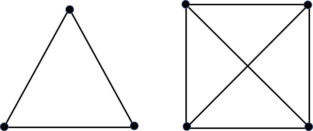
with . They stabilize an -qubit graph state that is local-unitary equivalent to the GHZ state . The simplest example of such a graph state is associated with a complete three vertex graph (left of Fig. 1) state which is stabilized by the following three stabilizing operators:
| (8) |
and can be stated as
| (9) | |||||
The next simplest set of stabilizers of this form is associated with a connected four vertex graph (on the right of Fig. 1) and in a similar way we can construct further such -qubit connected graph states.
II.4 Self-testing with temporal inequalities
In its original formulation put forward in Ref. Mayers and Yao (2004) (see also Ref. Šupić and Bowles (2020)), self-testing aims to certify an unknown quantum state and a set of measurements from the statistics obtained in an experiment, up to certain equivalences such as local isometries and additional of some extra degrees of freedom Mayers and Yao (2004). The self-testing based on Bell inequality violations is by definition device-independent as it does not, in general, require any assumption about the state and the measurements. However, in the case of contextuality-based certification one has to make an additional assumption that the measurements involved obey certain compatibility relations Bharti et al. (2019b), which in the case of Bell scenario is automatically satisfied due to the spatial separation between observers. In general it is dificult to certify in an experiment whether such compatibility relations are obeyed by the measurements. There exist other self-testing schemes based on the violation of non-contextual inequalities which do not require making this assumption Saha et al. (2020); Das et al. (2022).
Our aim here is to introduce the temporal-correlations version of the contextuality-based certification schemes introduced recently in Ref. Santos et al. (2022), which does not rely on any assumption about the compatility of the involved measurements. To this aim, let us consider a temporal inequality, say constructed from a non-contextuality inequality, , i.e., using the techniques in II.2. We have an experiment that realizes the sequential measurement scenario for , such that both the state (in general mixed) and measurements (in general non-projective) is unknown.
We then consider a reference experiment with a known pure state for some and known measurements acting on . We assume that our reference experiment also achieves the maximal quantum value of the given expression . With these two experiments at hand, we can now introduce the definition of self-testing in the case of contextuality or sequential scenarios that was put forward in Irfan et al. (2020):
Definition 2.
Suppose an unknown state and a set of measurements violate the temporal inequality maximally. Then, this maximal quantum violation self-tests the state and the set of measurements such that there exists exists a projection and a unitary acting on so that
| (10) |
Speaking alternatively, the above definition says that based on the observed non-classicality one is able to identify a subspace in on which all the observables act invariantly. Equivalently, can be decomposed as , where acts on , whereas acts on the orthogonal complement of in ; in particular, . Moreover, there exists a unitary .
III Self-testing of three-qubit complete graph state
III.1 Non-contextuality inequality
Taking inspiration from the previous works Irfan et al. (2020); Jebarathinam et al. (2023); Santos et al. (2022); Das et al. (2022), let us now introduce the following non-contextuality inequality for self-testing the complete graph state of three qubits and a set of nine observables:
| (11) |
where , and are dichotomic observables with eigenvalues and hence satisfy . Note that the notation for is such that and represent the same observable. This enables us to identify the symmetries of the inequality which are convenient for the later proofs.
It can be checked that the classical bound of the inequality (III.1) can be obtained by assigning the values to each variable , and which implies . And, the maximum algebraic value of is , which we can achieve with the following choice of quantum operators:
| (12) |
and the graph state in Eq. (9), where . In fact, to derive the inequality (III.1) we exploited the fact that the graph state is an eigenstate of each of the product of observables appearing in , except for for which it is an eigenvector with eigenvalue .
Notice also that for readability, we use a compact notation to represent the observables, eg., , and represent respectively the Pauli and matrices acting on -th qubit. As illustrations, for the following should read like, and . We note that these operators obey the following commutation relations for ,
| (13) |
as well as the following anti-commutation relations
| (14) |
We also notice that the non-contextuality inequality (III.1), respects certain symmetries. These symmetries can be listed as follows
| (15) | |||
In the next subsection, we propose a temporal non-contextuality inequality derived from the Eq. (III.1) using the techniques proposed in II.2. We will not assume the commutation relations from Eq. (III.1), rather, we will certify the relations listed in Eqs. (III.1) and (14) from the maximal violation of the proposed temporal inequality. Hence, the self-testing proof of the measurements and the graph state with the temporal non-contextuality inequality also applies to the self-testing proof using the non-contextuality inequality in (III.1).
III.2 Self-testing with the temporal inequality
The temporal inequality constructed from (III.1) has the following form
| (16) | |||||
It is direct to observe that the maximal quantum value of this expression which equals also the maximal algebraic value amounts to and is achieved by the same state and observables as the maximal quantum value of .
Our next task is to prove that the maximal quantum violation of the inequality (16) can be used for certification of the graph state (9) along with the observables in (12). To this aim, consider a quantum realization given by a pure state and a set of quantum observables and with acting on , where is some unknown Hilbert space. If the inequality in Eq. (16) is maximally violated for a pure state then all the expectation values in the inequality, except the permutations of , take the value +1. Moreover, we can also get the following set of relations
| (17) | ||||
| (18) | ||||
| (19) | ||||
| (20) |
where and by ‘ permutations’, we mean that the relations also hold for all possible permutation of the indices. Notice that although the inequality (16) does not respect the symmetries (15) of the non-contextuality inequality (III.1), the above relations (17)–(20) respect those symmetries, which is sufficient for our purpose. From the above relations, we can conclude that the following commutation relations hold on the state .
Lemma 1.
Suppose the maximal quantum violation of inequality (16) is observed. Then, for all , the operators , and satisfy the following commutation relations on the state ,
| (21) |
Proof.
To prove this statement we can exploit the fact that the maximal violation of inequality (16) implies that the relations in (17)–(20) are satisfied.
Next, we also prove the anti-commutation relations (14) between the operators when acting on the state .
Lemma 2.
Suppose the maximal quantum violation of inequality (16) is observed. Then, the operators , and along with the state satisfy the following relations
for all triples ,
Proof.
As in the case of the previous lemma we can again exploit the relations (17)–(20). Let us first observe that they lead to the following chain of relations:
| (24) | |||||
where the first equality follows from Eq. (18), whereas the second one from Eq. (17). Then, the third and fourth identities are consequences of Eqs. (20) and (17), respectively. The last equality follows from Eq. (17). This proves that for any .
Applying the same approach, we then have
| (25) | |||||
and
| (26) | |||||
which give the remaining anticommutation relations. A similar proof follows for .
Lemmas 1 & 2 establish thus commutation and anticommutation relations for the observables when acting on the state maximally violating our inequality. Let us notice that the identities (17)–(20) allow us to derive even more relations for the observables and the state:
| (27) |
. These relations will be useful for the later proofs.
Now, inspired by the approach of Ref. Irfan et al. (2020), we define a subspace
| (28) | |||||
and prove the following fact for it.
Lemma 3.
Let the maximal quantum violation of inequality (16) is observed, then, is an invariant subspace of all the observables , and for .
Proof.
In order to prove this lemma we use Lemmas 1 & 2 as well as the relations in Eqs. (17)–(20) and (III.2).
Let us begin with the first observable and notice that non-trivial actions of on the subspace elements are:
-
•
, which follows from Eq. (19). This relation also implies that .
-
•
, which is a consequence of the first identity in Eq. (III.2),
-
•
, which stems from Eq. (18). This relation implies also that .
-
•
.
Thus, the action of on every vector from produces a vector belonging to . By symmetry, the same conclusion can be drawn for and . Thus the subspace is invariant under the action of all ’s. Similarly, the invariance of subspace can be shown under the action all ’s.
Let us finally consider the observables . The first identity in Eq. (III.2) says that for any and , and therefore the action of on or results in vectors that manifestly belong to . It then follows from Lemmas 1 and 2 that either commutes or anti-commutes with and on the state which implies that the action of keeps the remaining vectors within up to a negative sign. This completes the proof.
It should be noticed that due to Eq. (III.2), the subspace stays the same if one replaces the last vector in Eq. (28) by or or .
An important consequence of Lemma 3 is that the underlying Hilbert space and all the observables giving rise to the maximal violation of inequality (16) split as , where is the orthogonal complement of in , and
| (29) |
where the hatted operators , and are defined on , that is, etc. with being a projection onto , whereas the remaining ones on . Since , and act trivially on , that is, , which means that the observed correlations giving rise to the maximal violation of the inequality (16) come solely from the subspace , in what follows we can restrict our attention to the operators , and .
First, from the fact that , and are observables obeying , it directly follows that , and are observables too and satisfy
| (30) |
where is the identity acting on . Second, Eq. (29) implies that the hatted observables must obey the same commutation relations as , , and . We prove the following two lemmas in Appendix B.
Lemma 4.
Suppose the maximal quantum violation of inequality (16) is observed. Then, the operators , and satisfy the following commutation relations ,
And lastly, it turns out that the anti-commutation relations in Lemma 2 also apply to the observables on the subspace .
Lemma 5.
Suppose the maximal quantum violation of the inequality (16) is observed. Then, the following anti-commutation relations hold ,
With Lemmas 4 and 5 at hand, we can now employ the standard approach that has already been used in many non-locality-based self-testing schemes Kaniewski (2016b); Kaniewski et al. (2019); Sarkar et al. (2021); Baccari et al. (2020b). Precisely, using this approach we can first infer that the dimension of the subspace is even. To see this, note that from the above anti-commutation relation between and , we have
| (31) |
which after taking trace on both sides simplify to . Similarly we can show that . It thus follows that both the eigenvalues of each observable , or have equal multiplicities. This clearly implies that the dimension is an even number, for some , and thus . On the other hand, since , one concludes that the possible values that can take are .
The fact that , and are traceless together with the fact that they obey the commutation and anticommutation relations established in Lemmas 4 and 5 imply that up to some unitary operation these operators are equivalent to , and , where and are the identity and some operator on with (see for instance appendix B in Ref. Kaniewski et al. (2019) for the proof of this statement). This observation is one of the key ideas behind the proof of the following lemma.
Lemma 6.
Suppose the maximal quantum violation of the inequality (16) is observed. Then, there exists a unitary operator acting on such that
| (32) |
Proof.
Using the result (Lemma 3) of Ref. Santos et al. (2022), we can show that there exists a unitary , acting on the subspace , such that the operators and have the form given in Lemma 6. Then, our task is to determine the form of the operators .
Let us then move to the observables and consider first the . Clearly, the "rotated" matrix can be decomposed as
| (33) |
where are some matrices. Now, it is direct to observe that the conditions that commutes with and anticommutes with implies that
| (34) |
Next, the conditions that commutes with and anticommutes with imply that the matrix must obey the following relations
| (35) |
Let us then decompose in the following way
| (36) |
where are some matrices. After plugging the above representation into Eq. (34), one easily finds that , and therefore
| (37) |
To finally fix one can exploit the fact that commutes with and anticommutes with which means that
| (38) |
The only matrix compatible with the above constraints is for some . However, since is a quantum observable such that , one has that . As a result,
| (39) |
Using then the same methodology one can then show that
| (40) |
for any triple , and thus under the action of the unitary operation , all the observables , and have the form given Eq. (6), which completes the proof.
We can now present one of the main results of this paper.
Theorem 1.
Proof.
A quantum state that belongs to a Hilbert space and a set of observables , , and acting on attain the maximal quantum violation of the inequality (16) if and only if they satisfy the set of relations (17)–(20). The algebraic relations induced by this set of equations let us prove Lemmas 2-6 which imply that there exists a projection and a unitary operation for which Eqs. (6) hold true.
From the above characterization of the observables, we can infer the form of the state . We will also fix the sign of all the observables . First, after plugging and into Eqs. (18), one finds that the latter are the stabilizing relations of the three-qubit complete graph state and thus . One then observes that Eqs. (17) can only be satisfied if the sign of each of the observables in Eq. (6) is . Thus, the state and observables maximally violating our inequality are of the form (1-42).
Notice that the statement in Theorem 1 involves a global unitary operation, and therefore it cannot be considered only a state certification, but rather simultaneous certification of both the state and measurements giving rise to the maximal violation of our inequality.
IV Self-testing of multi-qubit graph states
We will construct temporal non-contextual inequalities to certify multi-qubit quantum systems, without assuming any commutation relations between the operators. Importantly, the maximum violation of the new inequality will enable us to verify the required commutation relations. The new inequalities are such that the number of measurement operators grows polynomially with the number of qubits. However, the number of correlators grows rapidly with the number of qubits. The inequalities we propose generalize the inequalities given in Eqs. (III.1) and (16).
IV.1 New scalable non-contextuality inequalities
We present new scalable non-contextuality inequalities (analogous to the -qubit inequalities in Santos et al. (2022)) for which a temporal extension will enable self-testing the multi-qubit states and measurements. Consider a set of observables denoted by , and respectively, where and . These operators are assumed to obey the following commutation relations
| (43) |
where and . It should be noted that commutes with if or while commutes with if and . Therefore, it is evident that is the generalization of the observables for arbitrary -values. Also, note that .
We will now describe our construction of scalable non-contextuality inequalities. Consider correlators of the following types,
| (44) |
where , and on the right-hand side we added the number of different correlators of a given type. Let us provide a few words of explanation about these correlations. The correlators of the first type in (IV.1) are that involve two measurements and for all pairs and observables with and a single observable . The second type involves those correlators that consist of a single measurement and observables . Then, we have correlators containing observables , and for all triples of and observables at the remaining ’positions’. Lastly, the correlators are self-explanatory.
Using these correlators let us now construct our non-contextuality inequality for the -qubit case to be of the following form,
| (45) |
where the constants and have been added to make the numbers of correlators of different types equal (cf. inequality (III.1)), stands for the maximal classical value of . To estimate the latter we can follow the pattern that one might observe after considering the expressions in (III.1) and also and explicitly stated in Appendix A. Indeed, we notice that the contribution from first line of Eq. (IV.1) is equal to which is exactly equal to the contribution from second line. The last two lines contribute . Therefore, the classical upper bound of is
| (46) |
At the same time, the maximal algebraic and at the same time the maximal quantum value of the expression amounts to
| (47) |
and it is strictly larger than for any .
Note here that for the above inequality reproduces the one in Eq. (III.1) by replacing with . The inequality in Eq. (IV.1) is constructed in such a way so that for every three indices such that , we have an inequality of the form of Eq. (III.1). To understand the connection, we refer enthusiastic readers to Appendix A where we discuss in a more detailed way the case.
Now, coming back to the inequality (IV.1), we see that it is non-trivial for any , i.e., . To prove this, we note that the quantum bound can be attained by the following observables
| (48) |
where these operators obey the commutation relations given in Eq. (IV.1).
To use the inequality Eq. (IV.1) for certification of the state and measurements whenever the inequality is violated maximally, we note that the operators must also satisfy the following relations,
| (49) |
where these relations hold true for all possible permutations of operators. In the next section, we will use the above relations to obtain the form of operators and and the state. In fact, we will obtain the compatibility relations and the relations in (IV.1) from the maximum violation of the temporal version of the inequality (IV.2).
Also, note here that, we do not use the extant -qubit non-contextuality inequality from Ref. Santos et al. (2022) as its temporal extension does not certify all required commutations relations.
IV.2 Self-testing with temporal extension of n-qubit non-contextuality inequality
Using the similar prescription for , we construct the temporal version of the -qubit non-contextuality inequality (IV.1), by replacing the sequential expectation value terms with a sum of sequential correlations (2). The exact form of our -qubit temporal inequality is given by
| (50) |
We will now use the above inequality for certification of the complete graph states of any number of qubits, and the measurements , and given in Eq. (48). From the maximum violation of the above inequality, we have all the temporal expectation value terms in taking the value +1, except the expectation value terms of the form which takes the value -1. In other words, the maximal violations give us the relations in (IV.1). Using this we can prove the following lemma,
Lemma 7.
Suppose the maximal quantum violation of the inequality (IV.2) is observed. Then, the operators , and obey the following commutation relations,
where .
Proof.
The proof is analogous to the one of Lemma Firstly, we define and then, by using the relations in (IV.1), we can get the following relations which give the above commutators;
Note that the proof of is the same as the proof of because of the symmetry of with respect to its indices.
Moreover, we also have anti-commutation relations in the form of the following lemma.
Lemma 8.
Suppose the maximal quantum violation of the inequality (IV.2) is observed. Then, the operators , and obey the following anti-commutation relations,
Proof.
Again, we will be using the relations from (IV.1) for the proof. We have the following relations,
which gives the required anti-commutation relations. Note that the proof for is similar to .
Lemmas 7 and 8 thus establish commutation and anticommutation relations between observables on the state maximally violating our inequality. What is more, together with equations they enable and the relations in (IV.1), we can also claim the following relations,
| (51) |
Now we will use these relations to show that the following subspace is invariant under the action of the operators , and
| (52) | |||||
where for any and . In the simplest cases of and , the above construction gives
with . In particular, is exactly the same as the one defined in Eq. (28) by noticing that due to Eq. (18), with and .
This is the same subspace as was found in Irfan et al. (2020) for the -qubit scenario. Hence, the number of vectors spanning is which implies . In fact, we show later that .
Our aim now is to identify the form of the operators , , and projected onto the subspace . The method of the proof of self-testing is similar to that used in the case . In what follows, we prove the following lemma in Appendix C,
Lemma 9.
Suppose the maximal quantum violation of the inequality (IV.2) is observed. Then, the subspace of is invariant under the action of the operators , and for .
Now, lemma 9 implies that , and can be represented as a direct sum of two blocks,
where , and are projections of , and onto , that is , and with denoting the projector onto . On the other hand, , and are defined on the orthogonal complement of in the Hilbert space that we denote ; clearly, .
Importantly, , and act trivially on the subspace , in particular , and consequently it is enough for our purposes to characterize , and . Our first step to achieving this goal is to show that the following commutation and anti-commutation relations between the hatted operators hold. We prove these relations in Appendix C.
Lemma 10.
Suppose the maximal quantum violation of the inequality (16) is observed, then the following holds,
Lemma 11.
Suppose the maximal quantum violation of the inequality (16) is observed, then the bellow relations holds ,
Next, we are in a position to state the following results in a lemma which is a straightforward generalization of Lemma 6.
Lemma 12.
Suppose the maximal quantum violation of our inequality (IV.2) is observed. Then, there exists a unitary matrix acting on for which
| (53) |
Proof.
Thus, we are able to certify the measurements , , and , without assuming commutation relations between the observables. Moreover, as we can show that the dimension of is exactly , our inequalities can be seen as dimension witnesses: The dimension of the Hilbert space supporting a state and observables giving rise to the maximal violation of our inequalities must be at least . Now, we present the main result in the form of the following theorem.
Theorem 2.
If a quantum state and a set of dichotomic observables , and with give rise to the maximal violation of the temporal non-contextual inequality (IV.2), then there exists a projection with and a unitary acting on such that
| (54) |
where is the complete graph state of qubits.
Proof.
The state and observables acting on the Hilbert space attain the maximal quantum violation of the inequality (IV.2), if and only if, they satisfy the set of equations in (IV.1). The algebra induced by this set of equations allows us to prove Lemmas 9, 10, 11 and 12; in particular, it follows that there exists a projection and a unitary acting on such that the relations (12) holds. Then, we note that the first equation of (IV.1) is satisfied only if the the sign of each observables, in (12) is .
Now, we note that the stabilizing relations from the second equation of (IV.1) uniquely determine a state, , associated with the complete graph with vertices. Therefore, we prove the theorem.
V Conclusions
Quantum contextuality provides a unique avenue in extending the task of self-testing quantum devices to scenarios where entanglement is not necessary or spatial separation between the subsystems is not required (cf., Irfan et al. (2020); Saha et al. (2020); Maity et al. (2021); Santos et al. (2022); Bharti et al. (2019b); Das et al. (2022)). However, such contextuality-based certification schemes rely on the compatibility relations among the measurements involved and are thus generally hard to implement in practice.
In this paper, we overcome this limitation by using the temporal inequalities derived from the non-contextuality inequalities, such that the maximal violation of these new inequalities will certify these commutation relations among the said measurement observables. In what follows, we are able to show that the maximum violation of these temporal non-contextual inequalities can be used for the certification of multi-qubit graph states and the measurements.
Recently, we developed a similar method to certify a two-qubit maximally entangled state and measurements from the maximal violation of a temporal non-contextual inequality Jebarathinam et al. (2023). Moreover, we were also able to show that the scheme presented in Jebarathinam et al. (2023) is also robust to noise and small experimental errors. Since the certification schemes presented in both works are similar, we expect that the certification scheme presented in the current work is also robust to noise and small experimental errors.
Furthermore, it would be interesting to identify which other non-contextuality inequality-based self-testing schemes can be converted to temporal inequalities so that they can still be used for self-testing of the states and measurements. Further research is needed to improve the scalability of our scheme with the number of certified qubits.
acknowledgments
This work was supported by the Polish National Science Centre through the SONATA BIS project No. 2019/34/E/ST2/00369. SS acknowledges funding through PASIFIC program call 2 (Agreement No. PAN.BFB.S.BDN.460.022 with the Polish Academy of Sciences). This project has received funding from the European Union’s Horizon 2020 research and innovation programme under the Marie Skłodowska-Curie grant agreement No 847639 and from the Ministry of Education and Science of Poland.
References
- Raussendorf and Briegel (2001) R. Raussendorf and H. J. Briegel, Phys. Rev. Lett. 86, 5188 (2001).
- Kok et al. (2007) P. Kok, W. J. Munro, K. Nemoto, T. C. Ralph, J. P. Dowling, and G. J. Milburn, Rev. Mod. Phys. 79, 135 (2007).
- Shor (1995) P. W. Shor, Phys. Rev. A 52, R2493 (1995).
- Terhal (2015) B. M. Terhal, Rev. Mod. Phys. 87, 307 (2015).
- Borregaard et al. (2020) J. Borregaard, H. Pichler, T. Schröder, M. D. Lukin, P. Lodahl, and A. S. Sørensen, Phys. Rev. X 10, 021071 (2020).
- Hilaire et al. (2021) P. Hilaire, E. Barnes, and S. E. Economou, Quantum 5, 397 (2021).
- Lanyon et al. (2010) B. P. Lanyon, J. D. Whitfield, G. G. Gillett, M. E. Goggin, M. P. Almeida, I. Kassal, J. D. Biamonte, M. Mohseni, B. J. Powell, M. Barbieri, et al., Nature chemistry 2, 106 (2010).
- Ma et al. (2011) X.-s. Ma, B. Dakic, W. Naylor, A. Zeilinger, and P. Walther, Nature Physics 7, 399 (2011).
- Gaertner et al. (2007) S. Gaertner, C. Kurtsiefer, M. Bourennane, and H. Weinfurter, Phys. Rev. Lett. 98, 020503 (2007).
- Epping et al. (2017) M. Epping, H. Kampermann, C. macchiavello, and D. Bruß, New Journal of Physics 19, 093012 (2017).
- Thew et al. (2002) R. T. Thew, K. Nemoto, A. G. White, and W. J. Munro, Phys. Rev. A 66, 012303 (2002).
- Kiesel et al. (2005) N. Kiesel, C. Schmid, U. Weber, G. Tóth, O. Gühne, R. Ursin, and H. Weinfurter, Phys. Rev. Lett. 95, 210502 (2005).
- Mayers and Yao (2004) D. Mayers and A. Yao, Quantum Inf. Comput 4, 273–286 (2004).
- Šupić and Bowles (2020) I. Šupić and J. Bowles, Quantum 4, 337 (2020).
- Kaniewski (2016a) J. Kaniewski, Phys. Rev. Lett. 117, 070402 (2016a).
- Baccari et al. (2020a) F. Baccari, R. Augusiak, I. Šupić, J. Tura, and A. Acín, Phys. Rev. Lett. 124, 020402 (2020a).
- Panwar et al. (2022) E. Panwar, P. Pandya, and M. Wieśniak, arXiv preprint arXiv:2202.06908 (2022).
- Kochen and Specker (1967) S. Kochen and E. P. Specker, J. Math. Mech. 17, 59 (1967).
- Leggett and Garg (1985) A. J. Leggett and A. Garg, Phys. Rev. Lett. 54, 857 (1985).
- Budroni and Emary (2014) C. Budroni and C. Emary, Phys. Rev. Lett. 113, 050401 (2014).
- Brierley et al. (2015) S. Brierley, A. Kosowski, M. Markiewicz, T. Paterek, and A. Przysiężna, Phys. Rev. Lett. 115, 120404 (2015).
- Bharti et al. (2019a) K. Bharti, M. Ray, A. Varvitsiotis, N. A. Warsi, A. Cabello, and L.-C. Kwek, Phys. Rev. Lett. 122, 250403 (2019a).
- Irfan et al. (2020) A. A. M. Irfan, K. Mayer, G. Ortiz, and E. Knill, Phys. Rev. A 101, 032106 (2020).
- Saha et al. (2020) D. Saha, R. Santos, and R. Augusiak, Quantum 4, 302 (2020).
- Maity et al. (2021) A. G. Maity, S. Mal, C. Jebarathinam, and A. S. Majumdar, Phys. Rev. A 103, 062604 (2021).
- Santos et al. (2022) R. Santos, C. Jebarathinam, and R. Augusiak, Phys. Rev. A 106, 012431 (2022).
- Bharti et al. (2019b) K. Bharti, M. Ray, A. Varvitsiotis, N. A. Warsi, A. Cabello, and L.-C. Kwek, Phys. Rev. Lett. 122, 250403 (2019b).
- Das et al. (2022) D. Das, A. G. Maity, D. Saha, and A. S. Majumdar, Quantum 6, 716 (2022).
- Jebarathinam et al. (2023) C. Jebarathinam, G. Sharma, S. Sazim, and R. Augusiak, arXiv e-prints , arXiv:2307.06710 (2023), arXiv:2307.06710 [quant-ph] .
- Majidy et al. (2021) S. Majidy, J. J. Halliwell, and R. Laflamme, Phys. Rev. A 103, 062212 (2021).
- Pan et al. (2018) A. K. Pan, M. Qutubuddin, and S. Kumari, Phys. Rev. A 98, 062115 (2018).
- Markiewicz et al. (2014) M. Markiewicz, P. Kurzyński, J. Thompson, S.-Y. Lee, A. Soeda, T. Paterek, and D. Kaszlikowski, Phys. Rev. A 89, 042109 (2014).
- Hein et al. (2006) M. Hein, W. Dür, J. Eisert, R. Raussendorf, M. Nest, and H.-J. Briegel, arXiv preprint quant-ph/0602096 (2006).
- Gottesman (1996) D. Gottesman, Phys. Rev. A 54, 1862 (1996).
- Kaniewski (2016b) J. Kaniewski, Phys. Rev. Lett. 117, 070402 (2016b).
- Kaniewski et al. (2019) J. Kaniewski, I. Šupić, J. Tura, F. Baccari, A. Salavrakos, and R. Augusiak, Quantum 3, 198 (2019).
- Sarkar et al. (2021) S. Sarkar, D. Saha, J. Kaniewski, and R. Augusiak, npj Quantum Inf. 7, 151 (2021).
- Baccari et al. (2020b) F. Baccari, R. Augusiak, I. Šupić, J. Tura, and A. Acín, Phys. Rev. Lett. 124, 020402 (2020b).
Appendix A The special case of of non-contextual inequality (IV.1)
The non-contextual inequality (IV.1) is constructed in such a way that for every index , we have an inequality of the form of Eq. (III.1). We explain it by expanding the inequality for ,
| (55) |
Rearranging the terms in so that for the four sets of three indices, we have one of the four expressions,
| (56) |
From the above form, it is clear that consists of four expressions of the form (III.1). For example, when and in Eqs. (IV.1), we have the following terms for
where we see that we have a sitting in from of all the terms from inequality (III.1) except for terms. Likewise, we have three other expressions. Therefore, it is direct to find that .
Appendix B Commutation and anti-commutation relations for hatted operators in three-qubit scenario
The proof of Lemma 4.– If we can show that the operators , , and follow the aforementioned commutation relations on the subspace , it would also immediately imply the commutation relations for the hatted operators. Now consider the commutators acting on so that appear together in any sequential correlation terms in inequality (16). We can always get the following from the relations (17)-(20) which contain all the possible permutations. So in the following, we exclude such trivial scenarios and will consider only those commutators and subspace vectors so that the operators do not appear together in any sequential correlation terms in inequality (16).
For the commutation , we find that the following relation is the only non-trivial one to show,
which follows from from Eq. (18), (Eq. 17) and (Eq. III.2). Similarly, for , we need to show the following two relations only. First one is
using from Eq. (18), from Eq. (17) and from Eq. (III.2). And the second one is found to be
using from Eq. (III.2), from Eq. (19) and from Eq. (17). Next, for , we need to prove three non-trivial cases. We first have
using from Eq. (18), from Eq. (19) and from Eq. (III.2). It is easy to see that a similar proof works for . Further, we can see that following holds
by using and from Eq. (18). Lastly, we find below one
For , we show the following relation
using from Eq. (III.2) and and from Eq. (LABEL:3qubitallpermutations). Next,
by considering and from Eq. (III.2). Lastly, we have which follows a similar arguments. It is also clear that the above proofs work equally for , as the operator is symmetric with respect to the exchange of indices. Now, for , we show
holds using and from Eq. (III.2)). Then, one can prove following
by utilizing from Eq. (III.2), and from Eq. (LABEL:3qubitallpermutations).
For , we have the following four non-trivial commutation relations. First one being
using , from Eq. (III.2), , , , and from Eq. (17)-(19). Second, we show
using , , from Eq. (17)-(19) and from Eq. (III.2). Third, one can deduce that the below relation
does hold as , , , , from Eq. (17)-(19) and from Eq. (III.2). Finally, it is easy to show that
holds using , from Eq. (III.2), plus its permutations, and from Eqs. (17)-(18).
The proof of Lemma 5.– As we had proven for the commutators, if we can show that the anti-commutators from Lemma 2 hold on the subspace , then the anti-commutation relations will also hold for the hatted operators. For , we need to consider five non-trial cases. The first one,
follows using and from Eq. (III.2). Then, one shows
using , , from Eq. (18)-(19). Next, we find that
holds using the relation and from Eq. (III.2). Further, we find the following relation
using , , , and from Eq. (18)-(19); and lastly,
follows using from Eq. (III.2). Then for , we need to show the following relations. We can prove following
using and from Eq. (III.2). Next one is
using , , , , and from Eq. (17)-(19). Then, we show the following holds
utilizing from Eq. (17), from Eq. (19) and from Eq. (III.2). Further, we show
using , from Eq. (III.2), from Eq. (18), from Eq. (19); and lastly,
using from Eq. (III.2), from Eq. (19) and from Eq. (17). Next for , we can show
by using and from Eq. (III.2), from Eq. (18) and from Eq. (20);
using , , , , , and from Eq. (17)-(19);
utilizing , from Eq. (III.2), , and from Eq. (18);
using and from Eq. (III.2);
by using , from Eq. (III.2), and from Eq. (18);
utilizing , , , , , and from Eq. (17)-(19); and lastly,
Finally, we notice that a proof for holds similarly to .
Appendix C Invariant subspace, commutation and anti-commutation relations for hatted operators in -qubit scenario
The proof of Lemma 9.– We have the following by using from Eq. (IV.1) and from Eq. (IV.2),
| (57) |
Then, by using from Eq. (IV.2), we also have the following relations,
| (58) |
These two identities are crucial for the proof of the lemma. We will consider the different cases separately as follows.
Action of on : Let us first consider the following different cases when acts on on . Using relation from Eq. (IV.1), we find
where for and . Then we notice the following hold for ,
where the first equality comes from Eq. (57). The second and last equality comes from (Eq. IV.2) and (Eq. IV.1) respectively. Thus, keeps the state in for . Now, for the cases with where , first, we consider , and find that the following hold,
where we used the fact that is equivalent to under permutation from Eq. (IV.1). The last case for , we show
where we get the first equality from (58), then used from Eq. (IV.2) and from Eq. (IV.1) for immediate steps. Thus the subspace is invariant under the action of operators for any .
Action of on : We consider the action of operators on in different cases. For the cases with where and , we find
where . We get above relation using permutations of from Eq. (IV.1) by moving the operators and towards the right. Then, for , we get
where the first equality follows from Eq. (57) and last one using from Eq. (IV.2). Lastly, for with and , we show the following
where we used the various permutations of from Eq. (IV.2). Therefore keeps invariant.
Action of on : Finally, we will consider the action of operators on in different cases. Let us assume with and , then we have
using the permutations of the identity from Eq. (IV.1). And, whenever or for , we find
where using the permutations of the identity s.t., , and the identity from Eq. (IV.1). Now, the scenario when both and are equal to one of the ’s with , we find
using the permutations of the identity , then from Eq. (IV.1) and the permutations of from Eq. (IV.2). Next, we get from Eq. (58)
by using the identity from Eq. (IV.2) for the first equality and the permutations of from Eq. (IV.1) for the second one. Lastly, using Eq. (IV.2) in Eq. (57) we find , where can be the same or different from . Thus, keeps invariant.
The proof of Lemma 10.– Similar to the proof of Lemma 4, we can show that the commutators of unhatted operators vanish on all the subspace elements. Again if the operators appear together in inequality (IV.2), seeing holds, we ignore such scenarios in the -qubit case also. We consider acting on , for a demonstration, the remaining commutators can be proven similar to the Lemma 4.
For or with and , we find using from Eq. (IV.1),
where the second equality comes from using Eq. (IV.1). When both are equal to some we have
using , and the permutations of from Eq. (IV.1). Therefore, .
The proof of Lemma 11.– For the anti-commutators, we will show the proof for for a demonstration, and the remaining follows similar to Lemma 5.
Using from Eq. (58) for , we have by using from Eq. (IV.2) twice. Similarly, for , we have
using , and from Eq. (IV.1). Then, using Eq. (57) and from Eq. (IV.2), we have
Note that the following two cases don’t appear in the case of Lemma 5, and therefore, we consider them to complete the proof. Considering a state of the form with , we have
where and we use the permutations of , , and from Eq. (IV.1). Lastly, we find the below relation on the same state with
using the fact that , , the permutations of , and from Eq. (IV.1).