Deep Privacy Funnel Model:
From a Discriminative to a Generative Approach
with an Application to Face Recognition

Abstract

In this study, we apply the information-theoretic Privacy Funnel (PF) model to the domain of face recognition, developing a novel method for privacy-preserving representation learning within an end-to-end training framework. Our approach addresses the trade-off between obfuscation and utility in data protection, quantified through logarithmic loss, also known as self-information loss. This research provides a foundational exploration into the integration of information-theoretic privacy principles with representation learning, focusing specifically on the face recognition systems. We particularly highlight the adaptability of our framework with recent advancements in face recognition networks, such as AdaFace and ArcFace. In addition, we introduce the Generative Privacy Funnel ($\mathsf{GenPF}$) model, a paradigm that extends beyond the traditional scope of the PF model, referred to as the Discriminative Privacy Funnel ($\mathsf{DisPF}$). This $\mathsf{GenPF}$ model brings new perspectives on data generation methods with estimation-theoretic and information-theoretic privacy guarantees. Complementing these developments, we also present the deep variational PF (DVPF) model. This model proposes a tractable variational bound for measuring information leakage, enhancing the understanding of privacy preservation challenges in deep representation learning. The DVPF model, associated with both $\mathsf{DisPF}$ and $\mathsf{GenPF}$ models, sheds light on connections with various generative models such as Variational Autoencoders (VAEs), Generative Adversarial Networks (GANs), and Diffusion models. Complementing our theoretical contributions, we release a reproducible PyTorch package, facilitating further exploration and application of these privacy-preserving methodologies in face recognition systems. The source code will be made available upon acceptance at: https://gitlab.idiap.ch/biometric/deep-variational-privacy-funnel.

Keywords: Information-theoretic privacy, statistical inference, privacy funnel models, information obfuscation, face recognition systems, representation learning.

Corresponding Author: Behrooz Razeghi

1 Introduction

1.1 Motivation

(a)

(b)

Figure 1: High-level schematic comparison of privacy funnel models: (a) discriminative (classical) paradigm; (b) generative paradigm.

In the evolving landscape of face recognition technology, a critical issue has emerged: the need to balance privacy preservation with the utility of data. This challenge is particularly acute in the context of representation learning, where protecting individual privacy often conflicts with the demand for high-quality data analysis. Existing solutions in privacy-preserving representation learning face recognition approaches do not address the inherent information-theoretic trade-off between privacy and utility. This gap in the existing approaches underscores the importance of exploring new methodologies that can pave the way to understanding, quantifying and mitigating privacy risks for face recognition systems.

Our research introduces a novel approach to this problem by applying the information-theoretic Privacy Funnel (PF) model to face recognition systems. We propose a new method for privacy-preserving representation learning within an end-to-end training framework. This approach quantifies the trade-off between obfuscation and utility through logarithmic loss, generalizable to other loss functions for positive measures, effectively integrating the principles of information-theoretic privacy with face recognition technology. The adaptability of our framework with recent advancements in face recognition networks, including AdaFace and ArcFace, highlights its relevance and applicability in current technological contexts.

Distinguishing our approach from conventional methods, we introduce the Generative Privacy Funnel ($\mathsf{GenPF}$) model and the Deep Variational Privacy Funnel (DVPF) framework. The $\mathsf{GenPF}$ model extends beyond the traditional scope of Privacy Funnel analysis, offering new perspectives on data generation with privacy guarantees. Concurrently, the DVPF model provides a variational bound for measuring information leakage, enhancing the understanding of privacy challenges in deep representation learning. Additionally, the proposed methodology can also be combined with prior-independent privacy-enhancing techniques like differential privacy, marrying both prior-dependent and prior-independent mechanisms.

1.2 Key Contributions

Our research makes the following contributions to the field:

• Overview of Data Privacy Paradigm: Our research presents an overview of the current landscape in data privacy, articulating a clear understanding of privacy risks and the methodologies for their identification, quantification, and mitigation. It methodically categorizes Privacy-Enhancing Technologies (PETs), distinguishing between prior-dependent and prior-independent mechanisms and their significance in the broader context of privacy protection. Part of this work serves as a brief, but foundational review, offering a synthesized perspective on the privacy risk management in digital environments, while also addressing the implications for biometric PETs.

• First Study of Privacy Funnel Analysis in Face Recognition Systems: To the best of our knowledge, our work is the first to apply privacy funnel analysis to modern face recognition systems. This study bridges the gap between information-theoretic privacy principles and the practical implementation of privacy-preserving representation learning, focusing specifically on advanced face recognition technologies. Our framework is also designed to be easily integrated with recently developed face recognition networks like AdaFace and ArcFace in a plug-and-play fashion.

• Proposition of the Generative Privacy Funnel Model: We introduce the Generative Privacy Funnel ($\mathsf{GenPF}$) model, setting it apart from the traditional Privacy Funnel, which we now term the Discriminative Privacy Funnel ($\mathsf{DisPF}$) model. The $\mathsf{GenPF}$ model offers new insights into the generation of synthetic data with estimation-theoretic and information-theoretic privacy guarantees. We further explore a specific formulation of the $\mathsf{GenPF}$ model, demonstrating its potential and effectiveness in privacy preservation within face recognition systems.

• Introduction of the Deep Variational Privacy Funnel Model: Our work also includes the development of the deep variational PF (DVPF) model. We present a tight variational bound for quantifying information leakage, which provides a deeper understanding of the complexities involved in privacy preservation during deep variational PF learning. The DVPF model sheds light on connections with various generative models, such as the VAE family, GAN family, and Diffusion models. Furthermore, we have applied the DVPF model to the advanced face recognition systems.

• Versatile Data Processing Capabilities: Our model can process both raw image samples and embeddings derived from facial images.

1.3 Outline

We explore the data privacy paradigm in Sec. 2. In Sec. 3, we briefly introduce key preliminary concepts. Sec. 4 presents both the discriminative and generative perspectives of the PF model. We then present the deep variational PF model in Sec. 5. Experimental results related to face recognition systems can be found in Sec. 6, and our conclusions are drawn in Sec. 7.

1.4 Notations

Throughout this paper, random variables are denoted by capital letters (e.g., $X$, $Y$), deterministic values are denoted by small letters (e.g., $x$, $y$), random vectors are denoted by capital bold letter (e.g., $\mathbf{X}$, $\mathbf{Y}$), deterministic vectors are denoted by small bold letters (e.g., $\mathbf{x}$, $\mathbf{y}$), alphabets (sets) are denoted by calligraphic fonts (e.g., $\mathcal{X,Y}$), and for specific quantities/values we use sans serif font (e.g., $\mathsf{x}$, $\mathsf{y}$, $\mathsf{C}$, $\mathsf{D}$). Also, we use the notation $\left[N\right]$ for the set $\{1,2,\cdots,N\}$. $\mathrm{H}\left(P_{\mathbf{X}}\right)\coloneqq\mathbb{E}_{P_{\mathbf{X}}}\left[-\log P_{\mathbf{X}}\right]$ denotes the Shannon entropy; $\mathrm{H}\left(P_{\mathbf{X}}\|Q_{\mathbf{X}}\right)\coloneqq\mathbb{E}_{P_{\mathbf{X}}}\left[-\log Q_{\mathbf{X}}\right]$ denotes the cross-entropy of the distribution $P_{\mathbf{X}}$ relative to a distribution $Q_{\mathbf{X}}$; and $\mathrm{H}\left(P_{\mathbf{Z}\mid\mathbf{X}}\|Q_{\mathbf{Z}\mid\mathbf{X}}\mid P_{\mathbf{X}}\right)\coloneqq\mathbb{E}_{P_{\mathbf{X}}}\mathbb{E}_{P_{\mathbf{Z}\mid\mathbf{X}}}\left[-\log Q_{\mathbf{Z}\mid\mathbf{X}}\right]$ denotes the cross-entropy loss for $Q_{\mathbf{Z}\mid\mathbf{X}}$. The relative entropy is defined as $\mathrm{D}_{\mathrm{KL}}\left(P_{\mathbf{X}}\|Q_{\mathbf{X}}\right)\coloneqq\mathbb{E}_{P_{\mathbf{X}}}\big{[}\log\frac{P_{\mathbf{X}}}{Q_{\mathbf{X}}}\big{]}$. The conditional relative entropy is defined by $\mathrm{D}_{\mathrm{KL}}\left(P_{\mathbf{Z}\mid\mathbf{X}}\|Q_{\mathbf{Z}\mid\mathbf{X}}\mid P_{\mathbf{X}}\right)\coloneqq\mathbb{E}_{P_{\mathbf{X}}}\left[\mathrm{D}_{\mathrm{KL}}\left(P_{\mathbf{Z}\mid\mathbf{X}=\mathbf{x}}\|Q_{\mathbf{Z}\mid\mathbf{X}=\mathbf{x}}\right)\right]$ and the mutual information is defined by $\mathrm{I}\left(P_{\mathbf{X}};P_{\mathbf{Z}\mid\mathbf{X}}\right)\coloneqq\mathrm{D}_{\mathrm{KL}}\left(P_{\mathbf{Z}\mid\mathbf{X}}\|P_{\mathbf{Z}}\mid P_{\mathbf{X}}\right)$. We abuse notation to write $\mathrm{H}\left(\mathbf{X}\right)=\mathrm{H}\left(P_{\mathbf{X}}\right)$ and $\mathrm{I}\left(\mathbf{X};\mathbf{Z}\right)=\mathrm{I}\left(P_{\mathbf{X}};P_{\mathbf{Z}\mid\mathbf{X}}\right)$ for random objects $\mathbf{X}\sim P_{\mathbf{X}}$ and $\mathbf{Z}\sim P_{\mathbf{Z}}$. We use the same notation for the probability distributions and the associated densities.

2 Navigating the Data Privacy Paradigm

Data privacy is an ever-changing domain, propelled by the surge in personal and sensitive information production and exchange via digital platforms. Its primary objective is safeguarding the confidentiality, integrity, and availability of this information, restricting access and usage to authorized parties only. To realize this aim, data privacy employs various strategies and technologies such as encryption, access controls, and privacy-enhancing technologies (PETs). These methods aim to thwart unauthorized access and misuse of personal and sensitive data while minimizing the volume of information that is exposed or shared.

One of the key challenges in data privacy is managing the delicate balance between protecting personal and sensitive information and enabling its access and use for legitimate purposes. This trade-off becomes particularly challenging with rapid technological advances and the increasing demand for data-driven services. Another challenge is the absence of global standards and regulations for personal and sensitive information protection. Although many countries have established their own data privacy laws, the significant variations among these laws complicate the consistent protection of personal and sensitive data across borders. Despite these challenges, this field of data privacy is constantly evolving and advancing, with the development of new technologies and approaches to better protect personal and sensitive information.

The main challenge in the era of big data lies in balancing the utilization of data-driven machine learning algorithms with the crucial importance of protecting individuals’ privacy. The increasing volume of data collected and used for training machine learning algorithms raises concerns about potential misuse and privacy invasions. This situation presents several open problems, such as devising effective methods to anonymize data—ensuring individuals cannot be identified from training data—and developing robust technologies to safeguard personal information. Furthermore, there’s an imperative need to establish ethical guidelines for data use in machine learning, ensuring adherence to protect individuals’ rights.

2.1 Lunch with Turing and Shannon

Alan Turing visited Bell Labs in 1943, during the peak of World War II, to examine the X-system, a secret voice scrambler for private telephone communications between the authorities in London and Washington. While there, he met Claude Shannon, who was also working on cryptography. In a 28 July 1982 interview with Robert Price in Winchester, MA (Price, 1982), Shannon reminisced about their regular lunch meetings where they discussed computing machines and the human brain instead of cryptography (Guizzo, 2003). Shannon shared with Turing his ideas for what would eventually become known as information theory, but according to Shannon, Turing did not believe these ideas were heading in the right direction and provided negative feedback. Despite this, Shannon’s ideas went on to be influential in the development of information theory, which has had a significant impact on the fields of computer science and telecommunications.

Privacy has been a central concern in the fields of information theory and computer science since its inception. The interaction between Shannon and Turing highlights the different approaches taken by the two communities to address the issue of preventing unauthorized access to information contained in disclosed data. These approaches often involve the use of unique models and distinct mathematical techniques. It is important to note that these approaches have evolved over time as technology and threats to privacy have changed and continue to be an active area of research and development in both fields.

In the 1970s, two influential papers on privacy were published that highlighted the differences in approaches between information theory and computer science. The first paper, authored by Aaron Wyner while he was working at Bell Labs, introduced the concept of a wire-tap channel (Wyner, 1975), where data is transmitted over a discrete, memoryless channel (DMC) that is subject to interception by an eavesdropper, who is modeled as a second DMC observing the output of the first DMC. Wyner showed that it is possible to achieve perfect secrecy, or the ability to communicate without any information being disclosed to the interceptor, by designing codes that take advantage of the noise in the channel observed by the eavesdropper. This approach to privacy, which does not rely on assumptions about an adversary’s computational abilities and is often referred to as information-theoretic secrecy, became a key focus of research within the field of information theory.

In November 1976, Diffie and Hellman published a paper that introduced the concept of public key cryptography and described how it can be used to achieve secure communication without the need for a shared secret key (Hellman, 1976). This approach to cryptography, which is based on the difficulty of discovering private information without additional knowledge, such as a private key, ensures security against an adversary who is limited in their computational abilities. As a result, public key cryptographic systems are easier to implement and deploy compared to approaches that rely on information-theoretic secrecy, which do not make assumptions about an adversary’s computational capabilities. The paper also discussed public key distribution systems and verifiable digital signatures, which are important tools in ensuring the security of communication.

Since the publication of the papers on information theory and computer science approaches to privacy, public key cryptography, which assumes that an adversary is limited in their computational abilities, has become widely used in a variety of applications, including banking, healthcare, and public services. It is used billions of times a day in applications ranging from digital rights management to cryptocurrency. In contrast, information-theoretic approaches to secrecy, which do not make assumptions about an adversary’s computational capabilities, have been less successful in practical applications. Perfect secrecy against a computationally unbounded adversary requires strict assumptions, which can lead to elegant mathematical models but often result in security schemes that are difficult to implement in practice.

The intersection of information theory and computer science approaches to privacy continues to be relevant in today’s world, where the collection of individual-level data has increased significantly. This development has brought both challenges and opportunities for both fields, as the widespread collection of data has brought significant economic benefits, such as personalized services and innovative business models, but also poses new privacy threats. For example, social media posts may be used for undesirable political targeting (Effing et al., 2011; O’reilly et al., 2018), machine learning models may reveal sensitive information about the data used for training (Abadi et al., 2016), and public databases may be deanonymized with only a few queries (Narayanan and Shmatikov, 2008; Su et al., 2017). Both fields have faced new challenges and opportunities in addressing these issues.

2.2 Identification, Quantification, and Mitigation of Privacy Risks

Addressing privacy risks is paramount across all stages of personal data handling, including (i) collection, (ii) storage, (iii) processing, and (iv) sharing (dissemination). This comprehensive perspective ensures robust privacy protection applicable in various contexts, from traditional data management to advanced machine learning models. The growing body of research focused on managing privacy risks addresses three fundamental questions: ‘identification’, ‘quantification’, and ‘mitigation’ of these risks, setting the foundation for detailed exploration of state-of-the-art practices and methodologies in the field.

• Identification: How can we effectively identify the risk of data leakage and potential privacy attacks across the entire data lifecycle, from collection through to processing and sharing?

• Quantification: Following the identification of privacy risks, what metrics can be developed and applied to precisely quantify these risks and monitor the effectiveness of implemented privacy protection strategies?

• Mitigation: With a comprehensive understanding of privacy, what strategies can be formulated and implemented to mitigate identified risks, ensuring an optimal balance between operational objectives and privacy, in line with legal and ethical standards?

The following discussion will provide a brief exploration of these pivotal questions.

2.2.1 Identification of Privacy Risks

Identifying (understanding) privacy risks is a critical first step in safeguarding privacy across the entire data lifecycle, including collection, storage, processing, and dissemination (Solove, 2002, 2005). This task becomes increasingly vital and, at times, complex within the context of both traditional data management practices and the utilization of machine learning algorithms (Solove, 2010, 2024). The identification process requires a detailed understanding of potential vulnerabilities that could lead to data leakage and privacy attacks, alongside the development of systematic approaches to detect and assess these risks (Solove, 2010; Smith et al., 2011; Orekondy et al., 2017; Milne et al., 2017; Beigi and Liu, 2020). We briefly explore several key methodologies that are essential for the comprehensive identification of privacy risks in these areas.

Data Sensitivity Analysis:

Evaluating the inherent privacy risks associated with specific data types is fundamental in both conventional data management and machine learning contexts. This involves a meticulous assessment of datasets to identify data containing personally identifiable information or sensitive personal information. Through techniques such as attribute-based risk assessment and the application of privacy-preserving data mining principles, organizations can identify data elements that necessitate heightened protection measures. This analysis is crucial for setting the stage for privacy risk management, enabling a prioritized focus on the most sensitive data elements.

Vulnerability Assessment Across Data Lifecycle:

Conducting comprehensive vulnerability assessments is essential for identifying potential weaknesses that could lead to privacy breaches or violations. This process spans the entire data lifecycle, from initial data collection and storage to its processing and final dissemination. In the context of machine learning, this includes a detailed examination of model architectures, training procedures, and data processing pipelines to identify potential points of data leakage. Utilizing automated tools and frameworks for privacy audit and analysis plays a pivotal role in facilitating these comprehensive assessments, ensuring that vulnerabilities can be identified and addressed proactively.

Simulated Privacy Attack Scenarios:

Simulating potential privacy attacks is a proactive strategy for identifying vulnerabilities within both traditional data handling systems and machine learning models. Techniques such as adversarial modeling and synthetic data generation are employed to test the ease with which a model can be manipulated or data can be re-identified. This approach is particularly pertinent in the machine learning arena, where algorithms may be susceptible to specific privacy threats, including model inversion attacks and membership inference attacks. These simulated attack scenarios are invaluable for assessing the robustness of privacy protections and for highlighting areas where additional safeguards are needed.

2.2.2 Quantification of Privacy Risks

Following the identification of privacy risks and an in-depth understanding of the regulatory and ethical standards relevant to data privacy, it is crucial to precisely define and apply metrics. These metrics are indispensable for accurately quantifying the identified privacy risks and for diligently tracking progress towards their effective mitigation. Quantifying privacy risks requires the development of metrics that can precisely measure the severity of these risks across various stages of data handling, including collection, storage, processing, and dissemination. Importantly, the applicability and specificity of these metrics vary significantly based on the data lifecycle stage and the specific application context (Duchi et al., 2013a, 2014; Mendes and Vilela, 2017; Duchi et al., 2018; Wagner and Eckhoff, 2018; Bhowmick et al., 2018; Liao et al., 2019; Hsu et al., 2020; Bloch et al., 2021; Saeidian et al., 2021). This variability means that different metrics may have different operational interpretations (Issa et al., 2019; Kurri et al., 2023), necessitating a nuanced approach to their selection and implementation. These metrics act as definitive indicators of the privacy stance of data processing systems, enabling data custodians to make well-informed decisions about privacy risk management. We review a specific type of these quantitative metrics in Sec. 3.

2.2.3 Mitigation of Privacy Risks

In addressing the spectrum of privacy risks inherent in digital data handling, it’s imperative to employ a multifaceted strategy that encompasses both the theoretical frameworks and practical tools available for risk mitigation. Among these methodologies, PETs emerge as a critical subset, offering targeted solutions to protect personal data across its lifecycle. PETs are pivotal category of tools and methodologies designed to directly safeguard personal privacy by mitigating the risks associated with the collection, storage, processing, and sharing of personal data. PETs embody the principle of privacy by design, ensuring that privacy considerations are embedded within the infrastructure of digital technologies from the ground up. Deploying foundational techniques in PETs, such as pseudonymization (Chaum, 1981, 1985), anonymization (Sweeney, 2000, 2002), and encryption (Shannon, 1949; Diffie and Hellman, 1976; Hellman, 1977), directly addresses privacy risks by protecting data identifiability and integrity from collection to dissemination. We review PETs in Sec. 2.3.

2.3 Privacy-Enhancing Technologies

PETs play a vital role in safeguarding individual privacy by directly countering privacy threats. As adversaries constantly refine their methods, PETs become indispensable in the relentless pursuit to shield sensitive information from unauthorized access and misuse. Spanning a wide range, these technologies tackle various facets of privacy and data security.

2.3.1 Encryption, Anonymization, Obfuscation, and Information-Theoretic Technologies

These techniques are at the forefront of PETs, offering robust solutions to secure data whether it’s stored (at rest), being transmitted (in transit), or actively used (in use). Encryption technologies, encompassing both symmetric and asymmetric methods, as well as homomorphic encryption, serve as critical components by enabling secure data storage and transmission, along with the capacity for encrypted data processing. Complementing these are data pseudonymization (Chaum, 1981, 1985) and anonymization (Sweeney, 2000) techniques, which obscure personal identifiers, effectively anonymizing data to prevent direct association with individuals. Furthermore, differential privacy (Dwork et al., 2006b) introduces a probabilistic layer to data protection, injecting carefully calibrated noise to aggregated data or query outputs. This ensures that individual data points cannot be discerned, thereby protecting personal information from inference attacks within statistical datasets or when deploying machine learning models. Expanding upon these, information-theoretic privacy techniques offer a fundamental approach to data security by focusing on the maximum amount of information that can be gained by an adversary, regardless of the adversary’s computational power. By assessing the unpredictability and uncertainty in data, these methods ensure a theoretical limit on the information leakage, making them indispensable in scenarios where robust privacy guarantees are required, especially in the absence of assumptions about the adversary’s computational capabilities. In Sec. 2.4, we review these techniques from the standpoint of the prior knowledge we have regarding the data distribution.

2.3.2 Privacy-Preserving Computation Technologies

Secure computation techniques are essential for maintaining privacy during data processing (Yao, 1982; Micali and Rogaway, 1992; Mohassel and Rindal, 2018; Juvekar et al., 2018; Keller, 2020; Knott et al., 2021; Neel et al., 2021). Confidential computing (Mohassel and Rindal, 2018; Mo et al., 2022; Vaswani et al., 2023), which employs Trusted Execution Environments (TEEs) (Sabt et al., 2015), is a critical tool, isolating computation to protect data in use from both internal and external threats. Additionally, Secure Multi-party Computation (SMPC) (Goldreich, 1998; Du and Atallah, 2001; Cramer et al., 2015; Knott et al., 2021) facilitates collaborative computation over data distributed among multiple parties without revealing the data itself, enabling joint data analysis or model training while preserving the privacy of each party’s data. Zero-Knowledge Proofs (ZKPs) (Fiege et al., 1987; Kilian, 1992; Goldreich and Oren, 1994) offer another layer of security, allowing one party to prove the truth of a statement to another party without revealing any information beyond the validity of the statement itself, essential for scenarios requiring validation of data authenticity or integrity without exposing the data.

2.3.3 Decentralized Privacy Technologies

Decentralized privacy-preserving technologies encapsulate methods that enable collaborative and/or federated data analysis and model training across dispersed datasets without exposing the underlying data (Shokri and Shmatikov, 2015; McMahan et al., 2017; Dwivedi et al., 2019; Wei et al., 2020; Kaissis et al., 2020; Kairouz et al., 2021; Shiri et al., 2023). Federated learning exemplifies this approach by allowing machine learning models to be trained across various devices or servers. Rather than centralizing raw data, which could pose significant privacy risks, this technique involves aggregating model updates derived from local data. Such a decentralized approach not only maintains the confidentiality of individual contributions but also harnesses collective insights to improve model accuracy and performance, embodying the principles of privacy preservation in a distributed computing framework.

2.4 Prior-Dependent vs. Prior-Independent Mechanisms in PETs

There are two main types of privacy-enhancing mechanisms: ‘prior-independent’ and ‘prior-dependent’. Prior-independent mechanisms make minimal assumptions about the data distribution and the information held by an adversary and are designed to protect privacy regardless of the specific characteristics of the data being protected or the motivations and capabilities of any potential adversaries. Prior-dependent mechanisms, on the other hand, make use of knowledge about the probability distribution of private data and the abilities of adversaries in order to design privacy-preserving mechanisms. These mechanisms may be more effective in certain scenarios where the characteristics of the data and the adversary are known or can be reasonably estimated but may be less robust in situations where such information is uncertain or changes over time.

Data anonymization (Sweeney, 2000) techniques, such as $k$-anonymity (Sweeney, 2002), $\ell$-diversity (Machanavajjhala et al., 2006), $t$-closeness (Li et al., 2007), differential privacy (DP) (Dwork et al., 2006b), and pufferfish (Kifer and Machanavajjhala, 2012), aim to preserve the privacy of data through various forms of data perturbation. These techniques focus on queries, inference algorithms, and probability measures, with DP being the most popular context-free privacy notion based on the distinguishability of “neighboring” databases. However, DP does not provide any guarantee on the average or maximum information leakage (P. Calmon and Fawaz, 2012), and pufferfish, while able to capture data correlation, does not prioritize preserving data utility.

DP is a privacy metric that measures the impact of small perturbations at the input of a privacy mechanism on the probability distribution of the output. A mechanism is said to be $\epsilon$-differentially private if the probability of any output event does not change by more than a multiplicative factor $e^{\epsilon}$ for any two neighboring inputs, where the definition of “neighboring” inputs depends on the chosen metric of the input space. DP is prior-independent and often used in statistical queries to ensure the result remains approximately the same regardless of whether an individual’s record is included in the dataset. The privacy guarantee of DP can typically be achieved through the use of additive noise mechanisms, such as adding a small perturbation or random noise from a Gaussian, Laplacian, or exponential distribution (Dwork et al., 2014).

DP has been modified in various ways since its introduction, with variations including approximate differential privacy (which allows for a small additional parameter called delta) (Dwork et al., 2006a), local differential privacy (which assumes all inputs are neighboring) (Duchi et al., 2013b), and Rényi differential privacy (which uses Rényi divergence to measure the difference in output distributions from two neighboring inputs) (Mironov, 2017). DP has two key properties that make it useful for protecting privacy: (i) it is composable (Dwork et al., 2014; Abadi et al., 2016), meaning that the aggregate output of multiple observations from a DP mechanism still satisfies DP requirements; and (ii) it is robust to post-processing (Dwork et al., 2014), meaning that the output of a DP mechanism remains private even after further processing. These properties enable the modular construction and analysis of privacy mechanisms with a specific privacy leakage budget.

Information-theoretic (IT) privacy is the study of designing mechanisms and metrics that preserve privacy when the statistical properties or probability distribution of data can be estimated or partially known. IT privacy approaches (Reed, 1973; Yamamoto, 1983; Evfimievski et al., 2003; Rebollo-Monedero et al., 2009; P. Calmon and Fawaz, 2012; Sankar et al., 2013; P. Calmon et al., 2013; Makhdoumi and Fawaz, 2013; Asoodeh et al., 2014; P. Calmon et al., 2015; Salamatian et al., 2015; Basciftci et al., 2016; Asoodeh et al., 2016; Kalantari et al., 2017; Rassouli et al., 2018; Asoodeh et al., 2018; Rassouli and Gündüz, 2018; Liao et al., 2018; Osia et al., 2018; Tripathy et al., 2019; Hsu et al., 2019; Liao et al., 2019; Sreekumar and Gündüz, 2019; Xiao and Khisti, 2019; Diaz et al., 2019; Rassouli et al., 2019; Rassouli and Gündüz, 2019; Razeghi et al., 2020; Zarrabian et al., 2023; Zamani et al., 2023; Saeidian et al., 2023) model and analyze the trade-off between privacy and utility using IT metrics, which quantify how much information an adversary can gain about private features of data from access to disclosed data. These metrics are often formulated in terms of divergences between probability distributions, such as f-divergences and Rényi divergence. IT privacy metrics can be operationalized in terms of an adversary’s ability to infer sensitive data and can be used to balance the trade-off between allowing useful information to be drawn from disclosed data and preserving privacy. By using prior knowledge about the statistical properties of data and assumptions about the adversary’s inference capabilities, IT privacy can help to understand the fundamental limits of privacy and how to balance privacy and utility.

The IT privacy framework is based on the presence of a private variable and a correlated non-private variable, and the goal is to design a privacy-assuring mapping that transforms these variables into a new representation that achieves a specific target utility while minimizing the information inferred about the private variable. IT privacy approaches provide a context-aware notion of privacy that can explicitly model the capabilities of data users and adversaries, but they require statistical knowledge of data, also known as priors. This framework is inspired by Shannon’s information-theoretic notion of secrecy (Shannon, 1949), where security is measured through the equivocation rate at the eavesdropper, and by Reed (Reed, 1973) and Yamamoto’s (Yamamoto, 1983) treatment of security and privacy from a lossy source coding standpoint.

2.5 Challenges in Data-Driven Privacy Preservation Mechanisms

In the era of modern data-driven economies, cryptographic techniques, while foundational, face limitations in effectively addressing the spectrum of privacy risks. This limitation arises primarily because adversarial entities can directly observe disclosed data, complicating the protection of sensitive information. For instance, in scenarios where statisticians query databases containing sensitive information, merely encrypting outputs is insufficient. Such practices fail to prevent potential inference of private information through multiple queries, a challenge exemplified by the U.S. Census’ efforts to release population statistics without compromising individual privacy (Machanavajjhala et al., 2008). Similarly, in machine learning applications where user data is essential for model training, the dual-edged sword of data disclosure benefits and privacy risks becomes apparent. Here, the risk emerges from adversaries’ ability to extract individual-level information by analyzing the model’s responses.

The overarching objective in these data-centric contexts is not to eliminate information leakage entirely—a feat that is virtually unattainable against both computationally bounded and information-theoretic adversaries. Instead, the goal shifts towards achieving a demonstrable level of privacy that balances with utility. This nuanced approach stands in contrast to the absolute zero information leakage ideal of both cryptography and information-theoretic security models. Here, the privacy threat model envisages adversaries who scrutinize disclosed data to deduce sensitive information, such as political preferences or the presence of an individual within a dataset.

Emerging privacy mechanisms, spearheaded by advances in both computer science and information theory, eschew assumptions on the adversary’s computational prowess. These innovative approaches vary in the adversary’s inference objectives—ranging from probability of correct guesses to minimizing mean-squared reconstruction errors—and the modeling of private information. A critical challenge in this domain is the utility-privacy trade-off, which demands careful consideration of application-specific utility against privacy needs.

Among the vanguard of data-driven privacy solutions are mechanisms inspired by Generative Adversarial Networks (GANs). These strategies conceptualize privacy protection as a strategic game between a defender (or privatizer) and an adversary, where the privatizer’s goal is to encode datasets to thwart inference leakage regarding private or sensitive variables (Edwards and Storkey, 2016; Hamm, 2017; Huang et al., 2017; Tripathy et al., 2019; Huang et al., 2018). Meanwhile, the adversary endeavors to extract these variables from the released data. The optimization of privacy-preserving mechanisms through adversarial training—whether deterministic or stochastic—epitomizes the dynamic interplay between privacy protection and data utility.

As machine learning technologies evolve and become more pervasive, the imperative for robust, data-driven privacy mechanisms becomes increasingly critical. These privacy safeguards are indispensable for maintaining individual privacy, fostering public trust in organizations and governments, and mitigating the potential adverse effects of data breaches. Such breaches can lead to significant repercussions, including reputational damage, financial loss, and eroded trust in digital institutions. Thus, prioritizing the development and implementation of potent privacy-preserving strategies is paramount in safeguarding sensitive information in our increasingly data-centric world.

2.6 Threats to PETs

In this subsection, we briefly explore the challenges confronting PETs, reviewing the diverse types of attacks that seek to undermine the integrity and confidentiality of PETs. We discuss adversaries characterized by a broad range of objectives, as well as the strategies they utilize.

2.6.1 Adversary Objectives

Based on our understanding, we can classify the adversary objectives into three main categories: (i) data reconstruction, (ii) unauthorized access, and (iii) user re-identification.

Data Reconstruction:

The primary aim here is to accurately reconstruct original data from its encoded or protected form, whether through cryptographic, statistical-theoretic, information-theoretic, or estimation-theoretic privacy perspectives (Agrawal and Srikant, 2000; Rebollo-Monedero et al., 2009; Sankar et al., 2013; Asoodeh et al., 2016; Dwork et al., 2017; Bhowmick et al., 2018; Ferdowsi et al., 2020; Stock et al., 2022; Razeghi et al., 2023; Shiri et al., 2024). This encompasses two distinct goals. The first, ‘attribute-level recovery’ (micro goal), involves extracting specific attributes or features from protected data, ranging from demographic information to unique behavioral patterns. Adversaries might utilize these details for actions like impersonation, targeted phishing attacks, or information profiling. The second, ‘complete data reconstruction’ (macro goal), goes a step further. Here, adversaries aim to fully revert privacy-preserving measures to access entire datasets. This could entail piecing together fragmented personal data from multiple sources or decrypting encrypted information to reveal sensitive details, leading to potential misuses such as identity theft, financial fraud, or corporate espionage.

Unauthorized Access:

The objective here is for the adversary to gain access to systems, networks, or data to which they do not have permission or authorization (Dunne, 1994; Campbell et al., 2003; Winn, 2007; Mohammed, 2012; Muslukhov et al., 2013; Sloan and Warner, 2017; Razeghi et al., 2018; Maithili et al., 2018; Prokofiev et al., 2018; Wang et al., 2019). This can be for various purposes such as stealing sensitive data, disrupting system operations, planting malware, or conducting espionage. The underlying goal is to infiltrate a system or database without being detected and without having legitimate credentials or authorization.

User Re-identification:

The primary objective in user re-identification is the subtle linking of anonymized data back to identifiable individuals, despite the absence of direct identifiers (El Emam et al., 2011; Layne et al., 2012; Zheng et al., 2015; Henriksen-Bulmer and Jeary, 2016; Zheng et al., 2016; Ye et al., 2021). In this pursuit, adversaries are not just attempting to reveal identities but are actively aiming to undermine the integrity and purpose of data anonymization and privacy-preserving measures. Their efforts are directed toward establishing connections between seemingly unrelated, anonymized data sets and specific, identifiable individuals. This includes efforts aimed at correlating disjointed pieces of information to reconstruct identifiable profiles and, in more extended scenarios, to track individual behaviors and patterns over time. Such objectives pose significant privacy concerns, as they directly challenge the effectiveness of data anonymization techniques intended to protect individual identities and personal information.

2.6.2 Adversary Knowledge

Technical Model Insights:

The adversary may have a deep understanding of the computational models or algorithms used in the system. It encompasses comprehensive knowledge of model architecture, parameters, training methodologies, vulnerabilities, and potential ways to exploit them (Wang and Gong, 2018; Song et al., 2019; Oseni et al., 2021; Bober-Irizar et al., 2023; Yang et al., 2023). This includes detailed knowledge of the model’s architecture such as layers, neurons, weights, and activation functions, which enables pinpointing and exploiting inherent weaknesses or backdoors. Additionally, insights into the training regime, including epochs, learning rates, and loss functions, are crucial in informing the creation of attacks tailored to the model’s vulnerabilities.

Operational System Workflow:

Adversary knowledge in this area encompasses the overall operational workflow of the system, including system architecture, data flow, user interactions, security protocols, network infrastructure, third-party integrations, and external dependencies. A detailed understanding of this area can highlight areas of vulnerability. This includes tracing the data’s journey from inception to its ultimate storage or application to unearth vulnerabilities at various stages and discerning the nuances of the system’s decision-making process, particularly validation or rejection thresholds, to craft precision-targeted manipulative inputs.

Data and Information Profiling:

In this category, adversary insights into the data used by the system are covered. It includes understanding the types and sources of data, data processing methods, inherent biases, security measures for data protection, and potential data vulnerabilities. Important aspects are understanding the underlying structure and distribution of features within the dataset, including anomalies and edge cases, for designing bespoke attack vectors and analyzing even a limited subset of the true dataset to deduce the full dataset’s characteristics, particularly useful in reconnaissance attacks.

Security Mechanisms and Protocols:

This involves an understanding of the security measures in place, including authentication processes, encryption techniques, and other security protocols. Adversaries with this knowledge can plan attacks targeting specific weaknesses in the security setup.

Insider Operational Knowledge:

This includes knowledge acquired from having had legitimate access to the system or from detailed observations. It encompasses not just technical aspects but also operational procedures, organizational culture, and internal policies. This type of knowledge is particularly dangerous as it can lead to highly targeted and effective attacks.

2.6.3 Adversary Strategy

Adversary strategies span a wide array encompassing technical, systemic, data-centric, sociotechnical, and insider threats, to name a few, which cannot cover widely in our brief overview. From exploiting algorithmic vulnerabilities and cryptographic flaws to manipulating system infrastructures and communication protocols, these strategies reveal the depth and complexity of modern security challenges. Data-centric approaches further diversify these tactics through the exploitation of information leakage and the creation of synthetic identities. Privacy invasions leverage advanced traffic analysis and misuse of biometric data, while sociotechnical maneuvers utilize misinformation and target supply chains to undermine security indirectly. Insider and environmental manipulations, along with the exploitation of peripheral devices, underscore the necessity for comprehensive and integrated defense mechanisms. This extensive spectrum of adversary tactics necessitates advanced, multi-layered security measures that combine technological, procedural, and organizational strategies to counteract the evolving landscape of threats. In the context of machine learning and artificial intelligence, distinct vulnerabilities emerge. Below, we briefly review a couple of these strategies.

Gradient-Oriented Attacks:

In the gradient-oriented attacks, adversaries employ techniques to manipulate or infer the gradient calculations that are fundamental to machine learning models. These attacks are categorized into two main approaches: white-box and black-box attacks (Liu et al., 2016; Papernot et al., 2017; Ilyas et al., 2018; Bhagoji et al., 2018; Porkodi et al., 2018; Alzantot et al., 2019; Guo et al., 2019; Sablayrolles et al., 2019; Rahmati et al., 2020; Tashiro et al., 2020). In white-box attacks, attackers leverage detailed knowledge of the model’s architecture and parameters to either reverse-engineer the model or approximate the original training data, thus compromising the model’s decision-making process. This technique directly facilitates model inference attacks (Tramèr et al., 2016; Batina et al., 2019; Chandrasekaran et al., 2020), where the attacker’s goal is to uncover the model’s structure or deduce characteristics of the training data based on observable outputs or gradients. Black-box attacks contrast by not requiring direct access to the model’s internals. Instead, adversaries deploy probing techniques to estimate gradients and discern underlying data patterns, enabling them to infer critical insights about the model’s behavior and vulnerabilities. This method is particularly effective in membership inference attacks (Shokri et al., 2017), where the attacker aims to determine if specific data points were used in the model’s training set by observing the model’s predictions in response to crafted inputs.

Temporal Pattern Analysis:

Temporal pattern analysis involves scrutinizing temporal sequences in verification data to detect vulnerabilities (Kamat et al., 2009; Xiao and Xiong, 2015; Backes et al., 2016; Grover and Mark, 2017; Leong et al., 2020; Qi et al., 2020; Zhang et al., 2021; Li et al., 2023). Through sequential vulnerability detection, adversaries can highlight discernible patterns, potentially allowing them to predict when the system might introduce new noise or make updates, making their attacks more timely and effective. Time-based vulnerability exploitation leverages the analysis of temporal patterns in data processing, enabling adversaries to identify recurrent vulnerabilities or even predict system behavior at given times. This strategy could lead to targeted attacks during moments of predicted vulnerability or broad system disruptions during peak operation hours.

Comprehensive Synergy Attacks:

Comprehensive synergy attacks represent a multifaceted approach by integrating various data sources and modalities to uncover vulnerabilities and enhance the efficacy of attacks. This strategy can employ data gathered from eavesdropping, database interactions, and more. A critical component of this strategy is data poisoning (Biggio et al., 2012; Guo and Liu, 2020; Tian et al., 2022; Wang et al., 2022; Ramirez et al., 2022; Carlini et al., 2023), where adversaries deliberately introduce corrupted, misleading, or intentionally mislabeled data into the training set. The aim is to compromise the integrity of the machine learning model, leading to biased outcomes, incorrect predictions, or complete system failure. By corrupting the foundation of data on which models are trained, adversaries can significantly degrade the reliability and fairness of machine learning applications. Additionally, multi-modal synthesis (Abdullakutty et al., 2021; Liu et al., 2021; Hu et al., 2022) and noise reduction (Voloshynovskiy et al., 2000, 2001; Lu et al., 2002; Kloukiniotis et al., 2022; Chen et al., 2023) techniques are employed to augment data reconstruction efforts or manipulate verification procedures. For instance, denoising algorithms may be repurposed by adversaries to retrieve original, unaltered data, aiding in the generation of synthetic data for identity fraud. Through these comprehensive efforts, adversaries not only exploit existing vulnerabilities but also proactively create new ones, making it increasingly challenging to safeguard data and models against such attacks.

2.7 Biometric PETs

Biometric recognition systems automate individual identification through distinctive behavioral and biological traits. Biometric recognition systems fundamentally comprise four key subsystems: data capture, signal processing and feature extraction, comparison, and data storage. These subsystems work in unison to manage biometric data through its lifecycle, beginning with the capture of biometric samples, proceeding with the extraction of useful features, and concluding with the comparison and secure storage of biometric information. However, the security and privacy vulnerabilities inherent in face recognition systems, particularly through the potential reconstruction of face images from stored templates (embeddings), pose significant challenges.

Recent advancements have introduced a suite of Biometric Privacy-Enhancing Technologies (B-PETs), designed to safeguard sensitive information embedded within biometric templates. These techniques prioritize the protection of identity-related data, either by obscuring biometric templates through template protection schemes or by minimizing the inclusion of privacy-sensitive attributes such as age, gender, and ethnicity.

The ISO/IEC 24745 standard (ISO/IEC 24745:2022, E) sets forth four primary requirements for each biometric template protection scheme, encompassing the principles of cancelability, unlinkability, irreversibility, and the preservation of recognition performance. These biometric template protection schemes can be categorized into two main groups: (i) cancelable biometrics, which encompasses techniques like Bio-Hashing (Jin et al., 2004), MLP-Hash (Shahreza et al., 2023a), IoM-Hashing (Jin et al., 2017), among others, and rely on transformation functions dependent on keys to generate protected templates (Nandakumar and Jain, 2015; Sandhya and Prasad, 2017; Rathgeb et al., 2022), and (ii) biometric cryptosystems, which include methodologies such as fuzzy commitment (Juels and Wattenberg, 1999) and fuzzy vault (Juels and Sudan, 2006), either binding keys to biometric templates or generating keys from these templates (Uludag et al., 2004; Rathgeb et al., 2022). Additionally, some researchers have explored the application of Homomorphic Encryption for template protection in face recognition systems (Boddeti, 2018; Bassit et al., 2021; Shahreza et al., 2022).

Face recognition systems, as extensively discussed in prior research (Biggio et al., 2015; Galbally et al., 2010; Marcel et al., 2023), are not only susceptible to security threats but also face serious privacy vulnerabilities. These systems rely on facial templates extracted from face images, which inherently contain sensitive information about the individuals they represent. Recent studies have even demonstrated an adversary’s capability to reconstruct face images from templates stored within a face recognition system’s database (Shahreza and Marcel, 2023b, a).

To address the privacy concerns surrounding face recognition systems, numerous privacy-preserving methods have emerged in the literature. These privacy-enhancing techniques predominantly focus on protecting identity-related information within face templates through the utilization of template protection schemes (Razeghi et al., 2017; Boddeti, 2018; Rezaeifar et al., 2019; Mai et al., 2020; Hahn and Marcel, 2022; Shahreza et al., 2022, 2023b; Abdullahi et al., 2024), or on minimizing the inclusion of privacy-sensitive attributes, such as age, gender, ethnicity, among others, in these templates (Morales et al., 2020; Melzi et al., 2023).

2.8 Related Works

To address the most closely related works to ours, we consider two categories of research, which, while seemingly distinct, are indeed related. The first category encompasses research papers studying and analyzing the privacy funnel model, and the second comprises works addressing disentangled representation learning.

Considering the Markov chain $\mathbf{S}\hbox{$\--$}\kern-1.5pt\hbox{$\circ$}\kern-1.5pt\hbox{$\--$}\mathbf{X}\hbox{$\--$}\kern-1.5pt\hbox{$\circ$}\kern-1.5pt\hbox{$\--$}\mathbf{Z}$, the authors in (Hsu et al., 2020; de Freitas and Geiger, 2022; Huang and Gamal, 2024) tackle the privacy funnel problem. In (Hsu et al., 2020), the authors introduce a method to enhance privacy in datasets by identifying and obfuscating features that leak sensitive information. They propose a framework for detecting these information-leaking features using information density estimation, where features with information densities exceeding a predefined threshold are considered risky and are subsequently obfuscated. This process is data-driven, utilizing a new estimator known as the trimmed information density estimator (TIDE) for practical implementation.

In (de Freitas and Geiger, 2022), the authors present the conditional privacy funnel with side-information (CPFSI) framework. This framework extends the privacy funnel method by incorporating additional side information to optimize the trade-off between data compression and maintaining informativeness for a downstream task. The goal is to learn invariant representations in machine learning, with a focus on fairness and privacy in both fully and semi-supervised settings. Through empirical analysis, it is demonstrated that CPFSI can learn fairer representations with minimal labels and effectively reduce information leakage about sensitive attributes.

More recently, (Huang and Gamal, 2024) proposes an efficient solver for the privacy funnel problem by exploiting its difference-of-convex structure, resulting in a solver with a closed-form update equation. For cases of known distribution, this solver is proven to converge to local stationary points and empirically surpasses current state-of-the-art methods in delineating the privacy-utility trade-off. For unknown distribution cases, where only empirical samples are accessible, the effectiveness of the proposed solver is demonstrated through experiments on MNIST and Fashion-MNIST datasets.

In the domain of face recognition, the closest work to ours is (Morales et al., 2020), where the authors introduce a privacy-preserving feature representation learning approach designed to eliminate sensitive information, such as gender or ethnicity, from learned representations while maintaining data utility. This approach is centered around an adversarial regularizer that removes sensitive information from the learning objective.

Other fundamental related works include (Tran et al., 2017; Gong et al., 2020; Park et al., 2021; Li et al., 2022; Suwała et al., 2024), which primarily focus on disentangled representation learning and algorithmic fairness in face recognition systems. These works range from introducing methods to mitigate bias and improve pose-invariant face recognition to developing frameworks for disentangling data representation into specific types of information to mitigate discriminatory results in AI systems.

In (Tran et al., 2017), the authors introduce the disentangled representation learning generative adversarial network (DR-GAN) to address the challenge of pose variation in face recognition. Unlike conventional methods that either generate a frontal face from a non-frontal image or learn pose-invariant features, DR-GAN performs both tasks jointly through an encoder-decoder generator structure. This enables it to synthesize identity-preserving faces with arbitrary poses while learning a discriminative representation. The approach disentangles identity representation from other variations, such as pose, using a pose code for the decoder and pose estimation in the discriminator. DR-GAN can process multiple images per subject, fusing them into a single, robust representation and synthesizing faces in specified poses.

In (Gong et al., 2020), the authors present an approach to mitigating bias in automated face recognition and demographic attribute estimation algorithms, focusing on addressing the observed performance disparities across different demographic groups. They propose a de-biasing adversarial network, DebFace, which employs adversarial learning to extract disentangled feature representations for identity and demographic attributes (gender, age, and race) in a way that minimizes bias by reducing the correlation among these feature factors. Their approach combines demographic with identity features to enhance the robustness and accuracy of face representation across diverse demographic groups. The network comprises an identity classifier and three demographic classifiers, trained adversarially to ensure feature disentanglement and reduce demographic bias in both face recognition and demographic estimation tasks.

In (Park et al., 2021), the authors introduce a fairness-aware disentangling variational auto-encoder (FD-VAE) that aims to mitigate discriminatory results in AI systems related to protected attributes such as gender and age, without sacrificing beneficial information for target tasks. The FD-VAE model achieves this by disentangling data representation into three subspaces: target attribute latent (TAL), protected attribute latent (PAL), and mutual attribute latent (MAL), each designed to contain specific types of information. A decorrelation loss is proposed to appropriately align information within these subspaces, focusing on preserving useful information for the target tasks while excluding protected attribute information.

In (Li et al., 2022), the authors introduce Debiasing Alternate Networks (DebiAN) to mitigate biases in deep image classifiers without the need for labels of protected attributes, aiming to overcome the limitations of previous methods that require full supervision. DebiAN consists of two networks, a discoverer and a classifier, trained in an alternating manner to identify and unlearn multiple unknown biases simultaneously. This approach not only addresses the challenges of identifying biases without annotations but also excels in mitigating them effectively. The effectiveness of DebiAN is demonstrated through experiments on both synthetic datasets, such as the multi-color MNIST, and real-world datasets, showing its capability to discover and improve bias mitigation.

Recently, (Suwała et al., 2024) introduces PluGeN4Faces, a plugin for StyleGAN designed to manipulate facial attributes such as expression, hairstyle, pose, and age in images while preserving the person’s identity. It employs a contrastive loss to closely cluster images of the same individual in latent space, ensuring that changes to attributes do not affect other characteristics, such as identity.

In comparison to the research mentioned above, our work begins with a purely information-theoretic formulation of the PF model, which we have named the discriminative PF framework. We then extend the concept of the discriminative PF model to develop a generative PF framework. Building upon our objectives for PF frameworks, as grounded in Shannon’s mutual information, we present a tractable variational approximation for both our information utility and information leakage quantities. The variational approximation objectives we have obtained share some connections with the aforementioned research, thereby bridging the gap between information-theoretic approaches to privacy and privacy-preserving machine learning.

3 Preliminaries

3.1 General Loss Functions for Positive Measures

In data science, the representation of data via positive measures, including probability distributions, is critical. Positive measures are used extensively across various scientific fields, from modeling quantum states in physics to gene expression in biology, as well as representing wealth distribution in economics (Séjourné et al., 2023). Their role is further magnified in ML (Bishop and Nasrabadi, 2006; James et al., 2013), where data representation and manipulation rely on their approximation via discrete (e.g. histograms) or continuous (e.g. parameterized densities) models.

3.1.1 Divergences

Comparative analysis of measures in data science is facilitated by loss functions, which aim to quantify the similarity or dissimilarity between two measures. Rooted in distance-based methodologies, a special category of loss functions, known as divergences, are characteristically non-negative and definite. This means they are defined such that their value is zero if and only if the measures being compared are identical. Although the triangle inequality’s presence is a beneficial feature of these loss functions, imbuing them with a structure akin to metric spaces, it is not a universal prerequisite across all applications. Within this context, Csiszár’s concept of $\mathsf{f}$-divergences (Csiszár, 1967), a family of discrepancies between positive measures, becomes particularly relevant. They are defined by integrating pointwise comparisons of two measures and can be formalized as follows:

Definition 1 ($\mathsf{f}$-divergences)

Let $\mathsf{f}:\left(0,\infty\right)\rightarrow\mathbb{R}$ be a convex function which $\mathsf{f}(1)=0$. The $\mathsf{f}$-divergences between two probability measures $P$ and $Q$, $P\ll Q$ is defined as (Ali and Silvey, 1966; Csiszár, 1967):

$$\mathrm{D}_{\mathsf{f}}\left(P\|Q\right)\coloneqq\mathbb{E}_{Q}\left[\mathsf{f}\left(\frac{\mathrm{d}P}{\mathrm{d}Q}\right)\right].$$ (1)

Several specific instances of $\mathsf{f}$-divergences are of particular interest and have different ‘operational meanings’. Popular instances are defined as follows (Csiszár et al., 2004; Polyanskiy et al., 2010; Sharma and Warsi, 2013; Polyanskiy and Wu, 2014; Duchi, 2016):

1. Kullback-Leibler (KL) Divergence: The KL-divergence, $\mathrm{D}_{\text{KL}}(P\|Q)$, is a special case of $\mathsf{f}$-divergence where the function $\mathsf{f}$ is given by $\mathsf{f}(t)=t\log t$. It is expressed as $\mathrm{D}_{\mathsf{KL}}(P\|Q)\coloneqq\mathrm{D}_{\mathsf{f}}(P\|Q)$ for $\mathsf{f}(t)=t\log t$. It quantifies the amount of information lost when $Q$ is used to approximate $P$. It is widely used in scenarios like statistical inference.

2. Total Variation Distance: The total variation distance, denoted as $\mathsf{TV}(P,Q)$, is defined by $\mathsf{TV}(P,Q)\coloneqq\mathrm{D}_{\mathsf{f}}(P\|Q)$ with the function $\mathsf{f}$ being $\mathsf{f}(t)=|t-1|$. It is widely used in hypothesis testing and classification tasks in statistics, providing a bound on the maximum error probability.

3. Chi-squared ($\chi^{2}$) Divergence: The $\chi^{2}$-divergence, $\chi^{2}(P\|Q)$, is another form of $\mathsf{f}$-divergence given by $\chi^{2}(P\|Q)\coloneqq\mathrm{D}_{\mathsf{f}}(P\|Q)$ for the function $\mathsf{f}(t)=t^{2}-1$. It is usually used in statistical analysis for feature selection, particularly in the context of evaluating model fit and understanding feature importance. It is also used in estimation problems.

4. Squared Hellinger Distance: This measure, represented as $H^{2}(P,Q)$, employs the function $\mathsf{f}(t)=(\sqrt{2}-\sqrt{t})^{2}$ in its definition: $H^{2}(P,Q)\coloneqq\mathrm{D}_{\mathsf{f}}(P\|Q)$. This distance is particularly useful in Bayesian statistics. Unlike the KL-divergence, the Hellinger distance is symmetric and bounded.

5. Hockey-Stick Divergence: The hockey-stick divergence, denoted as $E_{\gamma}(P\|Q)$, is defined for a specific $\gamma$ (where $\gamma\geq 1$) and employs the function $\mathsf{f}(t)=(t-\gamma)_{+}$ with $(a)_{+}\coloneqq\max\{a,0\}$. Therefore, $E_{\gamma}(P\|Q)\coloneqq D_{\mathsf{f}}(P\|Q)$ for $\mathsf{f}(t)=(t-\gamma)_{+}$. This divergence can be particularly useful in decision-making models and risk assessments. The contraction coefficient of this divergence is also equivalent to the local Differential Privacy (Asoodeh et al., 2021).

Another important related loss is the Rényi divergence, which is not an $\mathsf{f}$-divergence but shares a similar purpose in measuring the discrepancy between probability distributions.

Rényi Divergence:

The Rényi divergence (Rényi, 1959, 1961) is denoted as $D_{\mathsf{R},\alpha}(P\|Q)$ for a parameter $\alpha$, where $\alpha\neq 1$ and $\alpha>0$. It is defined as:

$$D_{\mathsf{R},\alpha}(P\|Q)\coloneqq\frac{1}{\alpha-1}\log\left(\mathbb{E}_{Q}\left[\left(\frac{\mathrm{d}P}{\mathrm{d}Q}\right)^{\alpha}\right]\right).$$ (2)

This divergence provides a spectrum of metrics between distributions, with the parameter $\alpha$ controlling the sensitivity to discrepancies. The Kullback-Leibler divergence is a special case of Rényi divergence as $\alpha\rightarrow 1$. Rényi divergence finds extensive application in fields such as information theory, data privacy, cryptography, and machine learning, due to its adaptability and the comprehensive range of distributional differences it can capture.

3.1.2 Optimal Transport Distances

Optimal Transport (OT), a problem introduced by Gaspard Monge in the 18th century in his work ‘Mémoire sur la théorie des déblais et des remblais’ (Monge, 1781), emerges as a potent tool for probabilistic comparisons. It provides a uniquely flexible approach to gauge similarities and disparities between probability distributions, regardless of their supports.

Monge’s OT Problem:

Monge’s seminal problem seeks an optimal map $T:\mathcal{X}\rightarrow\mathcal{X}$ for transferring mass distributed according to a measure $\mu$ onto another measure $\nu$ on the same space $\mathcal{X}$. This problem can be metaphorically understood as finding the most efficient way to move sand to form certain patterns, with $\mu$ and $\nu$ representing the initial and desired distributions of sand, respectively. The key constraint in Monge’s formulation is represented by the equation $T_{\#}\mu=\nu$, where $T_{\#}$ denotes the push-forward operator. The integral equation defines the push-forward operator $\int_{\mathcal{X}}f\circ T\,\mathrm{d}\mu=\int_{\mathcal{X}}f\,\mathrm{d}\nu,\quad\forall f\in\mathcal{C}(\mathcal{X})$, where $\mathcal{C}(\mathcal{X})$ is the space of continuous functions on $\mathcal{X}$. This condition ensures that the measure $\mu$ is effectively transformed onto $\nu$ through the map $T$. Specifically, it implies that $T_{\#}\delta_{\mathbf{x}}=\delta_{T(\mathbf{x})}$ for Dirac measures $\delta_{\mathbf{x}}$ (Villani, 2008; Peyré et al., 2019; Séjourné et al., 2023).

In solving Monge’s problem, the objective is to find a measurable map $T$ that minimizes the total cost of transportation, subject to the aforementioned constraint. The cost of transporting a unit of mass from location $\mathbf{x}$ to location $\mathbf{y}$ in $\mathcal{X}$ is quantified by a cost function $\mathsf{c}(\mathbf{x},\mathbf{y})$. A typical choice for $\mathsf{c}(\mathbf{x},\mathbf{y})$, particularly in Euclidean spaces $\mathcal{X}=\mathbb{R}^{d}$, is the $p$-th power of the Euclidean distance, $\mathsf{c}(\mathbf{x},\mathbf{y})=\|\mathbf{x}-\mathbf{y}\|_{p}^{2}$. The original formulation by Monge is associated with linear transport costs, corresponding to $p=1$. However, the quadratic case where $p=2$ is often favored in modern applications due to its advantageous mathematical properties, including convexity and differentiability.

Definition 2 (OT Monge Formulation Between Arbitrary Measures)

Given two arbitrary (probability) measures $\mu$ and $\nu$ supported on $\mathcal{X}$ and $\mathcal{Y}$, respectively, the optimal transport Monge map $T^{\ast}$, if it exists, solves the following problem:

$$\inf_{T}\,\left\{\int_{\mathcal{X}}\mathsf{c}\left(\mathbf{x},T(\mathbf{x})\right)\,\mathrm{d}\mu(\mathbf{x}):\quad T_{\#}\mu=\nu\right\},$$ (3)

over $\mu$-measurable map $T:\mathcal{X}\rightarrow\mathcal{Y}$.

Kantorovich’s OT Problem:

Kantorovich’s formulation of the OT problem addresses the scenario of arbitrary measure spaces and introduces the concept of ‘mass splitting’ (Villani, 2008; Peyré et al., 2019; Séjourné et al., 2023). This innovative approach, initially developed by Kantorovich (Kantorovich, 1942) for applications in economic planning, significantly extends the framework of Monge’s problem. In Kantorovich’s formulation, the deterministic map $T$ of Monge’s problem is replaced by a probabilistic measure $\pi\in\Pi(\mu\times\nu)$, termed as a transport plan. Unlike Monge’s formulation where mass moves directly from a point $\mathbf{x}$ to $T(\mathbf{x})$, Kantorovich’s approach allows for the dispersion of mass from a single point $\mathbf{x}$ to multiple destinations. This flexibility makes it a generalized, or relaxed, version of Monge’s problem.

Definition 3 (Kantorovich’s OT Problem)

Let $\mathcal{X}$ and $\mathcal{Y}$ be two measurable spaces. Let $\mathcal{P}(\mathcal{X})$ and $\mathcal{P}(\mathcal{Y})$ be the sets of all positive Radon probability measures on $\mathcal{X}$ and $\mathcal{Y}$, respectively. For any measurable non-negative cost function $\mathsf{c}:\mathcal{X}\times\mathcal{Y}\rightarrow\mathbb{R}^{+}$, the Kantorovich’s OT problem between two positive measures $\mu\in\mathcal{P}(\mathcal{X})$ and $\nu\in\mathcal{P}(\mathcal{Y})$ is defined as:

$$\mathsf{OT}_{\mathsf{c}}\left(\mu,\nu\right)\coloneqq\mathop{\inf}_{\pi\in\Pi(\mu,\nu)}\int_{\mathcal{X}\times\mathcal{Y}}\mathsf{c}(\mathbf{x},\mathbf{y})\,\mathrm{d}\pi(\mathbf{x},\mathbf{y})=\mathop{\inf}_{\bm{\pi}\in\Pi(\mu,\nu)}\mathbb{E}_{\pi}\left[\,\mathsf{c}(\mathbf{X},\mathbf{Y})\,\right],$$ (4)

where $\Pi(\mu,\nu)$ denotes the set of joint distributions (couplings) over the product space $\mathcal{X}\times\mathcal{Y}$ with marginals $\mu$ and $\nu$, respectively. That is, for all measurable sets $\mathcal{A}\subset\mathcal{X}$ and $\mathcal{B}\subset\mathcal{Y}$, we have:

$$\Pi(\mu,\nu)\coloneqq\left\{\pi\in\mathcal{P}(\mathcal{X}\times\mathcal{Y}):\;\pi(\mathcal{A}\times\mathcal{Y})=\mu(\mathcal{A}),\,\pi(\mathcal{X}\times\mathcal{B})=\nu(\mathcal{B})\right\}.$$ (5)

Having established the preliminary concepts of $\mathsf{f}$-divergences and optimal transport distances as foundational tools in data science, we now direct our attention to employing these loss functions for the quantification of privacy leakage and utility performance.

3.2 Measuring Privacy Leakage and Utility Performance

We can define a generic privacy risk loss function as a functional tied to the joint distribution $P_{\mathbf{S},\mathbf{Z}}$, which quantifies the information leakage about $\mathbf{S}$ when $\mathbf{Z}$ is disclosed. Such a privacy risk loss function can be represented as $\mathcal{C}_{\mathsf{S}}:\mathcal{P}\left(\mathcal{S}\times\mathcal{Z}\right)\rightarrow\mathbb{R}^{+}\cup\{0\}$. Analogously, a well-characterized and task-specific generic utility performance loss function can be formulated as a functional of the joint distribution $P_{\mathbf{X},\mathbf{Z}}$, capturing the utility retained about $\mathbf{X}$ through the release of $\mathbf{Z}$. This utility performance loss function is denoted as $\mathcal{C}_{\mathsf{U}}:\mathcal{P}\left(\mathcal{U}\times\mathcal{Z}\right)\rightarrow\mathbb{R}^{+}\cup\{0\}$. We can define the $\mathsf{f}$-information between two random objects $\mathbf{X}$ and $\mathbf{Z}$ as $\mathrm{I}_{\mathsf{f}}\left(\mathbf{X};\mathbf{Z}\right)=\mathrm{D}_{\mathsf{f}}\left(P_{\mathbf{X,Z}}\|P_{\mathbf{X}}P_{\mathbf{Z}}\right)$, where $\mathrm{D}_{\mathsf{f}}\left(\cdot\|\cdot\right)$ represents the $\mathsf{f}$-divergence (Polyanskiy and Wu, 2014), serving as a measure for both privacy (obfuscation) and utility. Expanding this framework, Arimoto’s mutual information (Arimoto, 1977) could also be employed to assess information utility and privacy leakage. In this research, however, we focus on Shannon mutual information as our primary loss function.

4 Privacy Funnel Model: Discriminative and Generative Paradigms

4.1 Discriminative Privacy Funnel Method: Optimizing Information Extraction Under Privacy Constraints

Given two correlated random variables $\mathbf{S}$ and $\mathbf{X}$ with a joint distribution $P_{\mathbf{S,X}}$, the objective in the (classical) discriminative PF method (Makhdoumi et al., 2014) is to derive a representation $\mathbf{Z}$ for useful data $\mathbf{X}$ via a stochastic mapping $P_{\mathbf{Z}\mid\mathbf{X}}$, satisfying the following constraints:

• Formation of a Markov chain $\mathbf{S}\hbox{$\--$}\kern-1.5pt\hbox{$\circ$}\kern-1.5pt\hbox{$\--$}\mathbf{X}\hbox{$\--$}\kern-1.5pt\hbox{$\circ$}\kern-1.5pt\hbox{$\--$}\mathbf{Z}$,

• Maximization of the Shannon mutual information $\mathrm{I}(\mathbf{X};\mathbf{Z})$ in the representation $\mathbf{Z}$ of $\mathbf{X}$,

• Minimization of the Shannon mutual information $\mathrm{I}(\mathbf{S};\mathbf{Z})$ in the representation $\mathbf{Z}$ of $\mathbf{X}$.

The classical PF method thus addresses the trade-off between information leakage $\mathrm{I}\left(\mathbf{S};\mathbf{Z}\right)$ and the revealed useful information $\mathrm{I}\left(\mathbf{X};\mathbf{Z}\right)$. This trade-off is formally represented as:

$$\mathsf{DisPF\text{-}MI}\left(R^{\mathrm{s}},P_{\mathbf{S},\mathbf{X}}\right)\coloneqq\mathop{\sup}_{\begin{subarray}{c}P_{\mathbf{Z}\mid\mathbf{X}}:\\ \mathbf{S}\hbox{$\--$}\kern-1.5pt\hbox{$\circ$}\kern-1.5pt\hbox{$\--$}\mathbf{X}\hbox{$\--$}\kern-1.5pt\hbox{$\circ$}\kern-1.5pt\hbox{$\--$}\mathbf{Z}\end{subarray}}\mathrm{I}\left(\mathbf{X};\mathbf{Z}\right)\quad\mathrm{subject~{}to}\;\;\mathrm{I}\left(\mathbf{S};\mathbf{Z}\right)\leq R^{\mathrm{s}}.$$ (6)

The $\mathsf{DisPF\text{-}MI}$ curve is defined by the values $\mathsf{DisPF\text{-}MI}\left(R^{\mathrm{s}},P_{\mathbf{S},\mathbf{X}}\right)$ for different $R^{\mathrm{s}}$. We can use a Lagrange multiplier $\alpha\geq 0$ to represent the $\mathsf{DisPF\text{-}MI}$ problem by the associated Lagrangian functional:

$$\mathcal{L}_{\mathsf{DisPF\text{-}MI}}\left(P_{\mathbf{Z}\mid\mathbf{X}},\alpha\right)\coloneqq\mathrm{I}\left(\mathbf{X};\mathbf{Z}\right)-\alpha\;\mathrm{I}\left(\mathbf{S};\mathbf{Z}\right).$$ (7)

By creating a unique measure called the $\mathrm{I}$-Measure, we can geometrically represent the relationship among Shannon’s information measures (Yeung, 1991; Razeghi et al., 2023). Given that the Markov chain $\mathbf{S}\hbox{$\--$}\kern-1.5pt\hbox{$\circ$}\kern-1.5pt\hbox{$\--$}\mathbf{X}\hbox{$\--$}\kern-1.5pt\hbox{$\circ$}\kern-1.5pt\hbox{$\--$}\mathbf{Z}$ necessitates $\mathrm{I}\left(\mathbf{S};\mathbf{Z}\mid\mathbf{X}\right)=0$, the corresponding information diagram ($\mathrm{I}$-diagram) vividly illustrates this and is featured in Figure 3. Note that $\mathrm{I}\left(\mathbf{S};\mathbf{X};\mathbf{Z}\right)=\mathrm{I}\left(\mathbf{S};\mathbf{Z}\right)-\mathrm{I}\left(\mathbf{S};\mathbf{Z}\mid\mathbf{X}\right)=\mathrm{I}\left(\mathbf{S};\mathbf{Z}\right)\geq 0$.

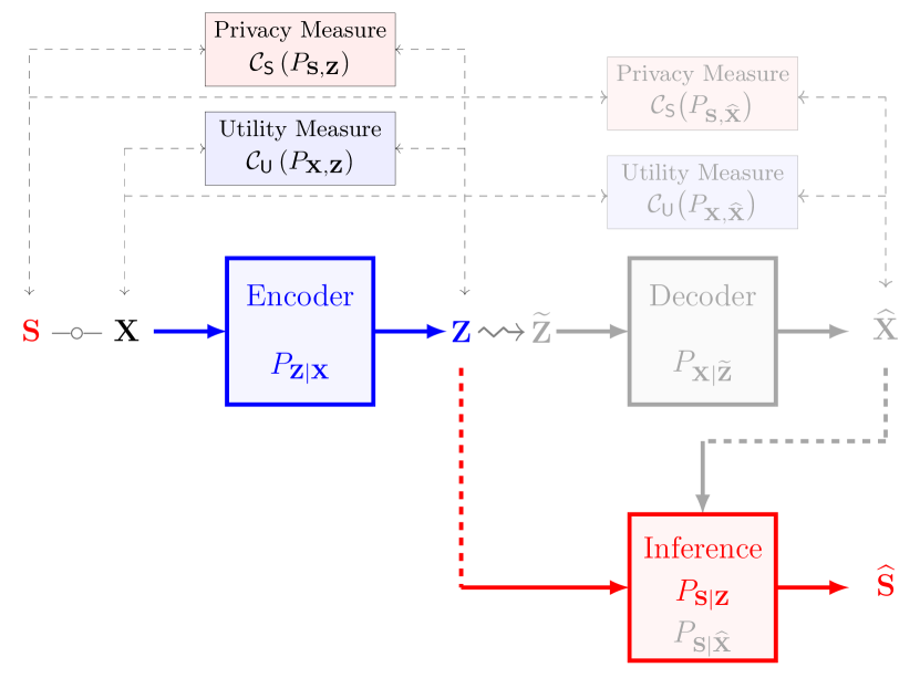
(a) Discriminative Privacy Funnel $\mathsf{DisPF}$.

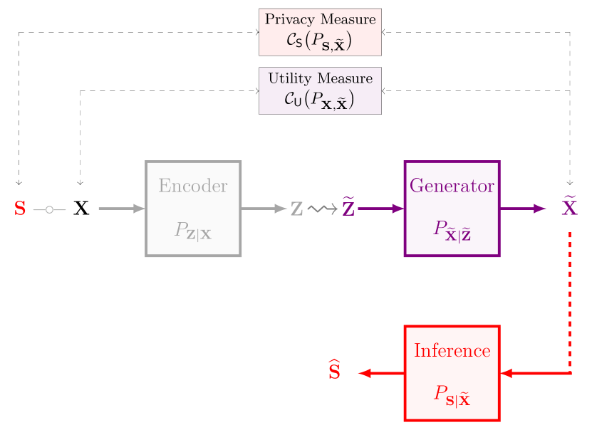
(b) Generative Privacy Funnel $\mathsf{GenPF}$.

Figure 2: Comparative overview of generalized privacy funnel (PF) approaches: (a) the established discriminative (classical) model; (b) the proposed generative model.

Discriminative Privacy Funnel with General Loss Functions:

Consider the extension of the standard discriminative PF objective to encompass a broader class of loss functions. The aim of this general discriminative PF approach is to obtain a representation $\mathbf{Z}$ for the useful data $\mathbf{X}$ via a probabilistic mapping $P_{\mathbf{Z}\mid\mathbf{X}}$. This objective is subject to the fulfillment of the following constraints:

• Establish a Markov chain $\mathbf{S}\hbox{$\--$}\kern-1.5pt\hbox{$\circ$}\kern-1.5pt\hbox{$\--$}\mathbf{X}\hbox{$\--$}\kern-1.5pt\hbox{$\circ$}\kern-1.5pt\hbox{$\--$}\mathbf{Z}$,

• Minimization of the utility performance loss function $\mathcal{C}_{\mathsf{U}}\left(P_{\mathbf{X},\mathbf{Z}}\right)$ via optimizing $\mathbf{Z}$ to preserve the useful information $\mathbf{X}$ pertinent to utility.

• Minimization of the privacy risk loss function $\mathcal{C}_{\mathsf{S}}\left(P_{\mathbf{S},\mathbf{Z}}\right)$ via optimizing $\mathbf{Z}$ to limit the leakage about sensitive information $\mathbf{S}$.

We can formulate this trade-off by imposing a constraint on one of the losses. Therefore, for a given information leakage constraint $R^{\mathrm{s}}\geq 0$, the trade-off can be encapsulated within a $\mathsf{DisPF}$ functional:

$$\mathsf{DisPF}\left(R^{\mathrm{s}},P_{\mathbf{S},\mathbf{X}}\right)\coloneqq\mathop{\inf}_{\begin{subarray}{c}P_{\mathbf{Z}\mid\mathbf{X}}:\\ \mathbf{S}\hbox{$\--$}\kern-1.5pt\hbox{$\circ$}\kern-1.5pt\hbox{$\--$}\mathbf{X}\hbox{$\--$}\kern-1.5pt\hbox{$\circ$}\kern-1.5pt\hbox{$\--$}\mathbf{Z}\end{subarray}} \mathcal{C}_{\mathsf{U}}\left(P_{\mathbf{X},\mathbf{Z}}\right)$$ (8)

$$\mathrm{subject~{}to}\quad\; \mathcal{C}_{\mathsf{S}}\left(P_{\mathbf{S},\mathbf{Z}}\right)\leq R^{\mathrm{s}}.$$

Any of the previously addressed general loss functions can be utilized in the above optimization problem.

Remark 1:

The discriminative PF model utilizes stochastic mapping $P_{\mathbf{Z}\mid\mathbf{X}}$ that can undertake either of the following processes: (i) A domain-preserving transformation, where, for example, in an image-to-image transition, the output image $\mathbf{Z}$ maintains the same domain but introduces specific alterations (such as noise or visual distortions) to obfuscate sensitive information of the original image $\mathbf{X}$. (ii) A non-domain-preserving transformation, as seen in methods like image-to-embedding, where the output $\mathbf{Z}$ is a more abstract form (an embedding) that provides a privacy-preserving representation of the original data $\mathbf{X}$, but in a different domain. The assessment of the obfuscated data’s ‘utility’ is performed either through direct analysis of $\mathbf{Z}$ using $\mathcal{C}_{\mathsf{U}}\left(P_{\mathbf{X},\mathbf{Z}}\right)$ or, where applicable, after a decoding phase (indicated in gray in 2(a)) using $\mathcal{C}_{\mathsf{U}}\big{(}P_{\mathbf{X},\mathbf{\widehat{X}}}\big{)}$. Information leakage is gauged by using measure $\mathcal{C}_{\mathsf{S}}\left(P_{\mathbf{S},\mathbf{Z}}\right)$, or in the case of decoded data, via $\mathcal{C}_{\mathsf{S}}\big{(}P_{\mathbf{S},\mathbf{\widehat{X}}}\big{)}$.

(a)

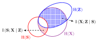
(b)

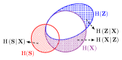
(c)

Figure 3: Information diagrams for $\mathbf{S}\hbox{$\--$}\kern-1.5pt\hbox{$\circ$}\kern-1.5pt\hbox{$\--$}\mathbf{X}\hbox{$\--$}\kern-1.5pt\hbox{$\circ$}\kern-1.5pt\hbox{$\--$}\mathbf{Z}$. (a) entropy $\mathrm{H}\left(\mathbf{S}\right)$, $\mathrm{H}\left(\mathbf{X}\right)$, $\mathrm{H}\left(\mathbf{Z}\right)$, and revealed useful (preserved) information $\mathrm{I}\left(\mathbf{X};\mathbf{Z}\right)$ and information leakage $\mathrm{I}\left(\mathbf{S};\mathbf{Z}\right)$; (b) residual information $\mathrm{I}\left(\mathbf{X};\mathbf{Z}\mid\mathbf{S}\right)$ and residual information $\mathrm{I}\left(\mathbf{S};\mathbf{X}\mid\mathbf{Z}\right)$; (c) private attribute uncertainty $\mathrm{H}\left(\mathbf{S}\!\mid\!\mathbf{X}\right)$, useful information decoding uncertainty $\mathrm{H}\left(\mathbf{X}\!\mid\!\mathbf{Z}\right)$, and encoding uncertainty $\mathrm{H}\left(\mathbf{Z}\!\mid\!\mathbf{X}\right)$.

4.2 Generative Privacy Funnel Method: Optimizing Data Synthesis Under Privacy Constraints

The Generative PF model aims to address the fundamental problem of synthetic data generation with privacy guarantees. Consider the general class of loss functions discussed in Sec. 3.2. The objective of the Generative Privacy Funnel model is to generate synthetic data, represented as $\mathbf{\widetilde{X}}$, from a latent code $\mathbf{\widetilde{Z}}$. This generation is achieved through a mapping (generator) $P_{\mathbf{\widetilde{X}}\mid\mathbf{\widetilde{Z}}}$, which can function in either a probabilistic or deterministic manner. The key goal of this model is to ensure that the synthetic data $\mathbf{\widetilde{X}}$ preserve useful information from the real data $\mathbf{X}$, necessary for a specific utility task while minimizing privacy leakage about sensitive data $\mathbf{S}$. This objective is subject to the fulfillment of the following constraints:

• Establish a Markov chain $\mathbf{\widetilde{Z}}\hbox{$\--$}\kern-1.5pt\hbox{$\circ$}\kern-1.5pt\hbox{$\--$}\mathbf{\widetilde{X}}\hbox{$\--$}\kern-1.5pt\hbox{$\circ$}\kern-1.5pt\hbox{$\--$}\mathbf{S}$,

• Minimization of the utility performance loss function $\mathcal{C}_{\mathsf{U}}\big{(}P_{\mathbf{X},\mathbf{\widetilde{X}}}\big{)}$ via optimizing $\mathbf{\widetilde{X}}$ to preserve the useful information $\mathbf{X}$ pertinent to utility.

• Minimization of the privacy risk loss function $\mathcal{C}_{\mathsf{S}}\big{(}P_{\mathbf{S},\mathbf{\widetilde{X}}}\big{)}$ via optimizing $\mathbf{\widetilde{X}}$ to limit the leakage about sensitive information $\mathbf{S}$.

We can formulate this trade-off as follows:

$$\mathsf{GenPF}\big{(}P_{\mathbf{S,\widetilde{X}}},R^{\mathrm{s}}\big{)}\coloneqq\mathop{\inf}_{\begin{subarray}{c}P_{\mathbf{\widetilde{X}}\mid\mathbf{\widetilde{Z}}}:\\ \mathbf{\widetilde{Z}}\hbox{$\--$}\kern-1.5pt\hbox{$\circ$}\kern-1.5pt\hbox{$\--$}\mathbf{\widetilde{X}}\hbox{$\--$}\kern-1.5pt\hbox{$\circ$}\kern-1.5pt\hbox{$\--$}\mathbf{S}\end{subarray}} \mathcal{C}_{\mathsf{U}}\big{(}P_{\mathbf{X},\mathbf{\widetilde{X}}}\big{)}$$ (9)

$$\mathrm{subject~{}to}\quad\; \mathcal{C}_{\mathsf{S}}\big{(}P_{\mathbf{S},\mathbf{\widetilde{X}}}\big{)}\leq R^{\mathrm{s}}.$$

Remark 2:

The objective of the generative PF model is on generating synthetic data that preserves the utility of the original dataset while ensuring constraints on sensitive information leakage. This model may optionally include an encoding step (represented in gray in 2(b)), or it may forego this step, opting to generate synthetic data directly from a latent noise domain.

Generative Privacy Funnel with Self-Information Loss Function:

The objectives of the $\mathsf{GenPF}$ model under self-information loss are as follows:

• Establish a Markov chain $\mathbf{\widetilde{Z}}\hbox{$\--$}\kern-1.5pt\hbox{$\circ$}\kern-1.5pt\hbox{$\--$}\mathbf{\widetilde{X}}\hbox{$\--$}\kern-1.5pt\hbox{$\circ$}\kern-1.5pt\hbox{$\--$}\mathbf{S}$,

• Maximization of the Shannon mutual information $\mathrm{I}\big{(}\mathbf{X};\mathbf{\widetilde{X}}\big{)}$ in the representation $\mathbf{\widetilde{X}}$ of $\mathbf{X}$,

• Minimization of the Shannon mutual information $\mathrm{I}\big{(}\mathbf{S};\mathbf{\widetilde{X}}\big{)}$ in the representation $\mathbf{\widetilde{X}}$ of $\mathbf{X}$.

$$\mathsf{GenPF\text{-}MI}\big{(}P_{\mathbf{S,\widetilde{X}}},R^{\mathrm{s}}\big{)}\coloneqq\mathop{\sup}_{\begin{subarray}{c}P_{\mathbf{\widetilde{X}}\mid\mathbf{\widetilde{Z}}}:\\ \mathbf{\widetilde{Z}}\hbox{$\--$}\kern-1.5pt\hbox{$\circ$}\kern-1.5pt\hbox{$\--$}\mathbf{\widetilde{X}}\hbox{$\--$}\kern-1.5pt\hbox{$\circ$}\kern-1.5pt\hbox{$\--$}\mathbf{S}\end{subarray}}\mathrm{I}\big{(}\mathbf{X};\mathbf{\widetilde{X}}\big{)}\quad\mathrm{subject~{}to}\;\;\mathrm{I}\big{(}\mathbf{S};\mathbf{\widetilde{X}}\big{)}\leq R^{\mathrm{s}}.$$ (10)

where $\mathbf{\widetilde{X}}=G\big{(}\mathbf{\widetilde{Z}}\big{)}$.

Remark 3:

The latent code $\mathbf{\widetilde{Z}}$ plays a versatile role in various generative models. It can represent the latent space in Variational Autoencoders (VAEs), be sampled from the $\mathcal{W}$ space in StyleGANs, derived through StyleGAN inversion methods, or constitute the latent space in diffusion models.

4.2.1 Generative Privacy Funnel in Face Recognition Systems

Creating an effective synthetic dataset for facial recognition systems demands integrating diverse demographic characteristics, encompassing varied ages, genders, ethnicities, and physical features, to enhance the system’s capability in recognizing and classifying a broad spectrum of human faces. Incorporating a range of facial expressions and poses, from happiness to neutrality, captured in different orientations like frontal and profile views, is critical for maintaining accuracy across various facial states. The dataset should also reflect diverse lighting and environmental conditions, including both indoor and outdoor settings, to ensure robust performance in real-world scenarios. High-resolution images are crucial for extracting detailed features, whereas incorporating lower-resolution images equips the system to handle suboptimal conditions. Including images of people wearing things like glasses or having part of their face covered is key to making sure we can recognize faces properly in all sorts of real-life situations. Accurate and consistent labeling is also a very important aspect to ensure reliable learning from the dataset. Ethical standards must be considered to prevent biases in image generation. Lastly, realism in synthetic imagery is imperative to replicate real-life scenarios accurately, as suboptimal image generation can significantly impair system performance. This holistic approach in dataset creation is vital for developing facial recognition systems that are not only robust and reliable but also versatile for diverse applications.

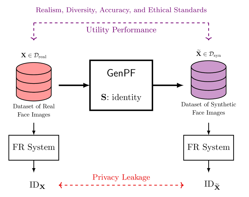
(a)

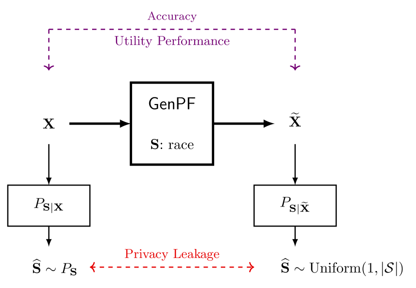
(b)

Figure 4: Visualization of the Generative Privacy Funnel in (a) face recognition systems and (b) face attribute recognition.

Incorporating the principles laid out in the comprehensive approach to synthetic dataset generation for facial recognition systems, the $\mathsf{GenPF}$ is aimed to generate synthetic images that not only adhere to the above-mentioned criteria but also protect the sensitive information from real dataset samples. This may include protecting personal identities as well as sensitive attributes such as gender, race, and emotion inherent in facial images. Moreover, $\mathsf{GenPF}$ has the potential to contribute to the creation of a balanced dataset, a crucial step in mitigating biases in face recognition systems. The specifics of this are discussed in Sec. 6.7.1

4.3 Threat Model

Our threat model includes the following assumptions:

• We consider an adversary who is interested in a specific attribute $\mathbf{S}$ related to the data $\mathbf{X}$. This attribute $\mathbf{S}$ could be any function of $\mathbf{X}$, possibly randomized. We limit $\mathbf{S}$ to a discrete attribute, which accommodates most scenarios of interest, such as a facial feature or an identity attribute.

• The adversary has access to the released representation $\mathbf{Z}$ and respects the Markov chain relationship $\mathbf{S}\hbox{$\--$}\kern-1.5pt\hbox{$\circ$}\kern-1.5pt\hbox{$\--$}\mathbf{X}\hbox{$\--$}\kern-1.5pt\hbox{$\circ$}\kern-1.5pt\hbox{$\--$}\mathbf{Z}$.

• We assume that the adversary knows the mapping $P_{\mathbf{Z}\mid\mathbf{X}}$ designed by the data owner (defender), i.e., the defender’s mechanism is public knowledge.

5 Deep Variational Privacy Funnel

In the following section, we delve into the heart of our methodology: Deep Variational Privacy Funnel.

5.1 Information Leakage Approximation

We provide parameterized variational approximations for information leakage, including an explicit tight variational bound and an upper bound. This approximation is designed to be computationally tractable and easily integrated with deep learning models, which allows for a flexible and efficient evaluation of privacy guarantees. To better understand the nature of information leakage, we can express $\mathrm{I}\left(\mathbf{S};\mathbf{Z}\right)$ as:

$$\mathrm{I}\left(\mathbf{S};\mathbf{Z}\right) =\mathrm{I}\left(\mathbf{X};\mathbf{Z}\right)-\mathrm{I}\left(\mathbf{X};\mathbf{Z}\mid\mathbf{S}\right)$$ (11a)

$$=\mathrm{I}\left(\mathbf{X};\mathbf{Z}\right)-\mathrm{H}\left(\mathbf{X}\mid\mathbf{S}\right)+\mathrm{H}\left(\mathbf{X}\mid\mathbf{S},\mathbf{Z}\right).$$ (11b)

The conditional entropy $\mathrm{H}\left(\mathbf{X}\mid\mathbf{S}\right)$ is originated from the nature of data since it is out of our control. It can be interpreted as ‘useful information decoding uncertainty’. Now, we derive the variational decomposition of $\mathrm{I}\left(\mathbf{X};\mathbf{Z}\right)$ and $\mathrm{H}\left(\mathbf{X}\mid\mathbf{S},\mathbf{Z}\right)$. The mutual information $\mathrm{I}\left(\mathbf{X};\mathbf{Z}\right)$ can be interpreted as ‘information complexity’ or ‘encoder capacity’ (Razeghi et al., 2023). It can be decomposed as:

$$\mathrm{I}\left(\mathbf{X};\mathbf{Z}\right) =\mathbb{E}_{P_{\mathbf{X},\mathbf{Z}}}\left[\log\frac{P_{\mathbf{Z}\mid\mathbf{X}}}{Q_{\mathbf{Z}}}\right]-\mathrm{D}_{\mathrm{KL}}\left(P_{\mathbf{Z}}\|Q_{\mathbf{Z}}\right)$$ (12a)

$$=\mathrm{D}_{\mathrm{KL}}\left(P_{\mathbf{Z}\mid\mathbf{X}}\|Q_{\mathbf{Z}}\mid P_{\mathbf{X}}\right)-\mathrm{D}_{\mathrm{KL}}\left(P_{\mathbf{Z}}\|Q_{\mathbf{Z}}\right),$$ (12b)

where $Q_{\mathbf{Z}}:\mathcal{Z}\rightarrow\mathcal{P}\left(\mathcal{Z}\right)$ is variational approximation of the latent space distribution $P_{\mathbf{Z}}$. The conditional entropy $\mathrm{H}\left(\mathbf{X}\!\mid\!\mathbf{S},\mathbf{Z}\right)$ can be decomposed as:

$$\mathrm{H}\left(\mathbf{X}\!\mid\!\mathbf{S},\mathbf{Z}\right)=-\mathbb{E}_{P_{\mathbf{S},\mathbf{X},\mathbf{Z}}}\left[\log P_{\mathbf{X}\mid\mathbf{S},\mathbf{Z}}\right] =-\mathbb{E}_{P_{\mathbf{S},\mathbf{X}}}\left[\mathbb{E}_{P_{\mathbf{Z}\mid\mathbf{X}}}\left[\log Q_{\mathbf{X}\mid\mathbf{S},\mathbf{Z}}\right]\right]-\mathrm{D}_{\mathrm{KL}}\left(P_{\mathbf{X}\mid\mathbf{S},\mathbf{Z}}\|Q_{\mathbf{X}\mid\mathbf{S},\mathbf{Z}}\right)$$ (13a)

$$\leq-\mathbb{E}_{P_{\mathbf{S},\mathbf{X}}}\left[\mathbb{E}_{P_{\mathbf{Z}\mid\mathbf{X}}}\left[\log Q_{\mathbf{X}\mid\mathbf{S},\mathbf{Z}}\right]\right]$$ (13b)

$$=\mathrm{H}\left(P_{\mathbf{X}\mid\mathbf{S,Z}}\|Q_{\mathbf{X}\mid\mathbf{S,Z}}\mid P_{\mathbf{S,Z}}\right)\eqqcolon\mathrm{H}^{\mathrm{U}}\!\left(\mathbf{X}\!\mid\!\mathbf{S},\mathbf{Z}\right),$$ (13c)

where $Q_{\mathbf{X}\mid\mathbf{S},\mathbf{Z}}\!:\!\mathcal{S}\!\times\!\mathcal{Z}\!\rightarrow\!\mathcal{P}\left(\mathcal{X}\right)$ is variational approximation of the optimal uncertainty decoder distribution $P_{\mathbf{X}\mid\mathbf{S},\mathbf{Z}}$, and the inequality in (13c) follows by noticing that $\mathrm{D}_{\mathrm{KL}}(P_{\mathbf{X}\mid\mathbf{S},\mathbf{Z}}\|Q_{\mathbf{X}\mid\mathbf{S},\mathbf{Z}})$ $\geq 0$. Using (11), (12) and (13), the variational upper bound of information leakage is given as:

$$\mathrm{I}\left(\mathbf{S};\mathbf{Z}\right)\leq\mathrm{D}_{\mathrm{KL}}\left(P_{\mathbf{Z}\mid\mathbf{X}}\|Q_{\mathbf{Z}}\mid P_{\mathbf{X}}\right)-\mathrm{D}_{\mathrm{KL}}\left(P_{\mathbf{Z}}\|Q_{\mathbf{Z}}\right)+\mathrm{H}^{\mathrm{U}}\!\left(\mathbf{X}\!\mid\!\mathbf{S},\mathbf{Z}\right).$$ (14)

Having the variational upper bound of information leakage, we now approximate the parameterized variational bound using neural networks. Let $P_{\bm{\phi}}(\mathbf{Z}\!\mid\!\mathbf{X})$ represent the family of encoding probability distributions $P_{\mathbf{Z}\mid\mathbf{X}}$ over $\mathcal{Z}$ for each element of space $\mathcal{X}$, parameterized by the output of a deep neural network $f_{\bm{\phi}}$ with parameters $\bm{\phi}$. Analogously, let $P_{\bm{\varphi}}\left(\mathbf{X}\!\mid\!\mathbf{S},\mathbf{Z}\right)$ denote the corresponding family of decoding probability distributions $Q_{\mathbf{X}\mid\mathbf{S},\mathbf{Z}}$, driven by $g_{\bm{\varphi}}$. Lastly, $Q_{\bm{\psi}}(\mathbf{Z})$ denotes the parameterized prior distribution, either explicit or implicit, that is associated with $Q_{\mathbf{Z}}$.

Using (12), the parameterized variational approximation of $\mathrm{I}\left(\mathbf{X};\mathbf{Z}\right)$ can be defined as:

$$\mathrm{I}_{\bm{\phi},\bm{\psi}}\left(\mathbf{X};\mathbf{Z}\right)\coloneqq\mathrm{D}_{\mathrm{KL}}\!\left(P_{\bm{\phi}}(\mathbf{Z}\!\mid\!\mathbf{X})\,\|\,Q_{\bm{\psi}}(\mathbf{Z})\mid P_{\mathsf{D}}(\mathbf{X})\right)-\mathrm{D}_{\mathrm{KL}}\!\left(P_{\bm{\phi}}(\mathbf{Z})\,\|\,Q_{\bm{\psi}}(\mathbf{Z})\right).$$ (15)

The parameterized variational approximation of conditional entropy $\mathrm{H}^{\mathrm{U}}\left(\mathbf{X}\mid\mathbf{S},\mathbf{Z}\right)$ in (13c) can be defined as:

$$\mathrm{H}_{\bm{\phi},\bm{\varphi}}^{\mathrm{U}}\left(\mathbf{X}\!\mid\!\mathbf{S},\mathbf{Z}\right)\coloneqq-\mathbb{E}_{P_{\mathbf{S},\mathbf{X}}}\left[\mathbb{E}_{P_{\bm{\phi}}(\mathbf{Z}\mid\mathbf{X})}\left[\log P_{\bm{\varphi}}(\mathbf{X}\!\mid\!\mathbf{S},\mathbf{Z})\right]\right].$$ (16)

Let $\mathrm{I}_{\bm{\phi},\bm{\xi}}\left(\mathbf{S};\mathbf{Z}\right)$ denote the parameterized variational approximation of information leakage $\mathrm{I}\left(\mathbf{S};\mathbf{Z}\right)$. Using (14), an upper bound of $\mathrm{I}_{\bm{\phi},\bm{\xi}}\!\left(\mathbf{S};\mathbf{Z}\right)$ can be given as:

$$\mathrm{I}_{\bm{\phi},\bm{\xi}}(\mathbf{S};\mathbf{Z})\;\leq\!\!\!\!\underbrace{\mathrm{I}_{\bm{\phi},\bm{\psi}}\left(\mathbf{X};\mathbf{Z}\right)}_{\mathrm{Information~{}Complexity}}\!\!+\!\underbrace{\mathrm{H}_{\bm{\phi},\bm{\varphi}}^{\mathrm{U}}\left(\mathbf{X}\!\mid\!\mathbf{S},\mathbf{Z}\right)}_{\mathrm{Information~{}Uncertainty}}\!\!\!\!+\,\mathrm{c}\eqqcolon\;\mathrm{I}_{\bm{\phi},\bm{\psi},\bm{\varphi}}^{\mathrm{U}}\left(\mathbf{S};\mathbf{Z}\right)+\mathrm{c},$$ (17)

where $\mathrm{c}$ is a constant term, independent of the neural network parameters.

This upper bound encourages the model to reduce both the information complexity, represented by $\mathrm{I}_{\bm{\phi},\bm{\psi}}\left(\mathbf{X};\mathbf{Z}\right)$, and the information uncertainty, denoted by $\mathrm{H}_{\bm{\phi},\bm{\varphi}}^{\mathrm{U}}\left(\mathbf{X}\!\mid\!\mathbf{S},\mathbf{Z}\right)$. Consequently, this leads the model to ‘forget’ or de-emphasize the sensitive attribute $\mathbf{S}$, which subsequently reduces the uncertainty about the useful data $\mathbf{X}$. In essence, this nudges the model towards an accurate reconstruction of the data $\mathbf{X}$.

(a)

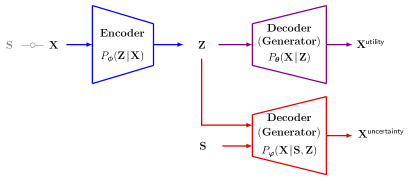
(b)

Figure 5: Core architectural components of the (a) deep discriminative privacy funnel and (b) deep generative privacy funnel models.

Now, let us derive another parameterized variational bound of information leakage $\mathrm{I}_{\bm{\phi},\bm{\xi}}\left(\mathbf{S};\mathbf{Z}\right)$. We can decompose $\mathrm{I}_{\bm{\phi},\bm{\xi}}\left(\mathbf{S};\mathbf{Z}\right)$ as follows:

$$\mathrm{I}_{\bm{\phi},\bm{\xi}}\left(\mathbf{S};\mathbf{Z}\right) =\mathbb{E}_{P_{\mathbf{S},\mathbf{X}}}\left[\mathbb{E}_{P_{\bm{\phi}}\left(\mathbf{Z}\mid\mathbf{X}\right)}\left[\log P_{\bm{\xi}}\left(\mathbf{S}\!\mid\!\mathbf{Z}\right)\right]\right]+\mathbb{E}_{P_{\mathbf{S}}}\left[\log P_{\bm{\xi}}(\mathbf{S})\right]-\mathbb{E}_{P_{\mathbf{S}}}\Big{[}\log\frac{P_{\mathbf{S}}}{P_{\bm{\xi}}(\mathbf{S})}\Big{]}$$ (18a)

$$=\underbrace{-\mathrm{H}_{\bm{\phi},\bm{\xi}}\left(\mathbf{S}\!\mid\!\mathbf{Z}\right)+\mathrm{H}\left(P_{\mathbf{S}}\,\|\,P_{\bm{\xi}}(\mathbf{S})\right)}_{\mathrm{Prediction~{}Fidelity}}\,\,\,-\!\!\!\!\underbrace{\mathrm{D}_{\mathrm{KL}}\left(P_{\mathbf{S}}\,\|\,P_{\bm{\xi}}(\mathbf{S})\right)}_{\mathrm{Distribution~{}Discrepancy}}$$ (18b)

$$\geq-\mathrm{H}_{\bm{\phi},\bm{\xi}}\left(\mathbf{S}\!\mid\!\mathbf{Z}\right)\,\,\,-\,\,\mathrm{D}_{\mathrm{KL}}\left(P_{\mathbf{S}}\,\|\,P_{\bm{\xi}}(\mathbf{S})\right)\eqqcolon\,\,\mathrm{I}_{\bm{\phi},\bm{\xi}}^{\mathrm{L}}\left(\mathbf{S};\mathbf{Z}\right),$$ (18c)

where $P_{\bm{\xi}}(\mathbf{S}\!\mid\!\mathbf{Z})$ denotes the corresponding family of decoding probability distribution $Q_{\mathbf{S}\mid\mathbf{Z}}$, where $Q_{\mathbf{S}\mid\mathbf{Z}}:\mathcal{Z}\rightarrow\mathcal{P}(\mathcal{S})$ is a variational approximation of optimal decoder distribution $P_{\mathbf{S}\mid\mathbf{Z}}$. Let us interpret the MI decomposition in Eq (18b):

• Negative Conditional Cross-Entropy $-\mathrm{H}_{\bm{\phi},\bm{\xi}}\left(\mathbf{S}\!\mid\!\mathbf{Z}\right)$: This term aims to maximize the uncertainty in predicting $\mathbf{S}$ given $\mathbf{Z}$. $\mathrm{H}_{\bm{\phi},\bm{\xi}}\left(\mathbf{S}\!\mid\!\mathbf{Z}\right)$ can be as low as $0$ when $\mathbf{S}$ is deterministically predictable given $\mathbf{Z}$. This means that knowing $\mathbf{Z}$ gives us full information about $\mathbf{S}$. A negative sign encourages the model (encoder) to increase the entropy of $\mathbf{S}$ given $\mathbf{Z}$, which means making $\mathbf{S}$ less predictable when you know $\mathbf{Z}$. In the case of a discrete sensitive attribute $\mathbf{S}$, the conditional entropy is maximized when all the conditional distributions $P_{\mathbf{S\mid\mathbf{Z}=\mathbf{z}}}$ are uniform. The maximum entropy is $\log_{2}|\mathcal{S}|$, where $|\mathcal{S}|$ is the number of possible states (or values, or classes) for $\mathbf{S}$. This means the adversary, lacking any additional information, can do no better than ‘random guessing’. This scenario equates to a potential lower boundary for $-\mathrm{H}_{\bm{\phi},\bm{\xi}}\left(\mathbf{S}\!\mid\!\mathbf{Z}\right)$ at $-\log_{2}|\mathcal{S}|$.

• Cross-Entropy $\mathrm{H}\left(P_{\mathbf{S}}\,\|\,P_{\bm{\xi}}(\mathbf{S})\right)$: This term encourages the classifier to produce correct predictions for $\mathbf{S}$. The minimum value is equal to the entropy of $P_{\mathbf{S}}$, i.e., $\mathrm{H}(P_{\mathbf{S}})$, which is achieved when $P_{\bm{\xi}}(\mathbf{S})=P_{\mathbf{S}}$. Given that $\mathbf{S}$ is discrete, the maximum value is $\log_{2}|\mathcal{S}|$.

• This term ensures the model’s inferred distribution, $P_{\bm{\xi}}(\mathbf{S})$, aligns tightly with the actual distribution $P_{\mathbf{S}}$. Ideally, the divergence measure, $\mathrm{D}_{\mathrm{KL}}\left(P_{\mathbf{S}}\|P_{\bm{\xi}}(\mathbf{S})\right)$, is minimized to zero when $P_{\bm{\xi}}(\mathbf{S})$ aligns perfectly with $P_{\mathbf{S}}$.

By pushing both $\mathrm{H}_{\bm{\phi},\bm{\xi}}\left(\mathbf{S}\!\mid\!\mathbf{Z}\right)$ and $\mathrm{H}\left(P_{\mathbf{S}}\,\|\,P_{\bm{\xi}}(\mathbf{S})\right)$ to their maximum values of $\log_{2}N$, and simultaneously minimizing distributional gap $\mathrm{D}_{\mathrm{KL}}\left(P_{\mathbf{S}}\,\|\,P_{\bm{\xi}}(\mathbf{S})\right)$, the mutual information $\mathrm{I}_{\bm{\phi},\bm{\xi}}\left(\mathbf{S};\mathbf{Z}\right)$ will approach zero, indicating that $\mathbf{Z}$ has minimal information about $\mathbf{S}$.

Using (17) and (18) we have:

$$-\mathrm{H}_{\bm{\phi},\bm{\xi}}\left(\mathbf{S}\!\mid\!\mathbf{Z}\right)-\mathrm{D}_{\mathrm{KL}}\left(P_{\mathbf{S}}\,\|\,P_{\bm{\xi}}(\mathbf{S})\right)\;\leq\;\mathrm{I}_{\bm{\phi},\bm{\xi}}(\mathbf{S};\mathbf{Z})\;\leq\;\mathrm{I}_{\bm{\phi},\bm{\psi}}\left(\mathbf{X};\mathbf{Z}\right)+\mathrm{H}_{\bm{\phi},\bm{\varphi}}^{\mathrm{U}}\left(\mathbf{X}\!\mid\!\mathbf{S},\mathbf{Z}\right)+\mathrm{c}.$$ (19)

The above lower and upper bounds lead us towards two alternative models. The upper bound in (19) encourages the model to directly minimizes the information complexity $\mathrm{I}_{\bm{\phi},\bm{\psi}}\left(\mathbf{X};\mathbf{Z}\right)$ as well as the information uncertainty $\mathrm{H}_{\bm{\phi},\bm{\varphi}}^{\mathrm{U}}\left(\mathbf{X}\!\mid\!\mathbf{S},\mathbf{Z}\right)$. By minimizing the information uncertainty $\mathrm{H}_{\bm{\phi},\bm{\varphi}}^{\mathrm{U}}\left(\mathbf{X}\!\mid\!\mathbf{S},\mathbf{Z}\right)$ the model forces to forget the sensitive attribute $\mathbf{S}$ at the expense of reducing the uncertainty about the original data $\mathbf{X}$, i.e., encourages the model to reconstruct the original data $\mathbf{X}$. In contrast, the lower bound in (19) encourages the model to maximizes (i) uncertainty about the sensitive attribute $\mathbf{S}$ given the released representation $\mathbf{Z}$, i.e., $\mathrm{H}_{\bm{\phi},\bm{\xi}}\left(\mathbf{S}\!\mid\!\mathbf{Z}\right)$, as well as (ii) the distribution discrepancy measure $\mathrm{D}_{\mathrm{KL}}\left(P_{\mathbf{S}}\,\|\,P_{\bm{\xi}}(\mathbf{S})\right)$. Note that minimizing the lower bound of information leakage may not necessarily minimize the average maximal possible leakage. Furthermore note that although the lower bound in (19) does not explicitly depend on the information complexity $\mathrm{I}_{\bm{\phi},\bm{\psi}}\left(\mathbf{X};\mathbf{Z}\right)$, it depends implicitly through the encoder $f_{\bm{\phi}}$.

5.2 Information Utility Approximation

In this subsection, we turn our focus on quantifying the utility of information. As with information leakage, we provide a careful decomposition of the mutual information $\mathrm{I}(\mathbf{X};\mathbf{Z})$ and derive a parameterized variational approximation for information utility. These measures form the foundation of the Deep Variational PF framework and pave the way for practical and scalable privacy preservation in deep learning applications. The end-to-end parameterized variational approximation associated to the information utility $\mathrm{I}(\mathbf{X};\mathbf{Z})$ can be defined as:

$$\mathrm{I}_{\bm{\phi},\bm{\theta}}\left(\mathbf{X};\mathbf{Z}\right) \coloneqq\mathbb{E}_{P_{\mathsf{D}}(\mathbf{X})}\left[\mathbb{E}_{P_{\bm{\phi}}\left(\mathbf{Z}\mid\mathbf{X}\right)}\Big{[}\log\frac{P_{\bm{\theta}}\left(\mathbf{X}\!\mid\!\mathbf{Z}\right)}{P_{\mathsf{D}}(\mathbf{X})}\Big{]}\right]$$ (20a)

$$=\mathbb{E}_{P_{\mathsf{D}}(\mathbf{X})}\left[\mathbb{E}_{P_{\bm{\phi}}\left(\mathbf{Z}\mid\mathbf{X}\right)}\left[\log P_{\bm{\theta}}\left(\mathbf{X}\!\mid\!\mathbf{Z}\right)\right]\right]-\mathrm{D}_{\mathrm{KL}}\left(P_{\mathsf{D}}(\mathbf{X})\,\|\,P_{\bm{\theta}}(\mathbf{X})\right)+\mathrm{H}\left(P_{\mathsf{D}}(\mathbf{X})\,\|\,P_{\bm{\theta}}(\mathbf{X})\right)$$ (20b)

$$\geq\underbrace{-\mathrm{H}_{\bm{\phi},\bm{\theta}}\left(\mathbf{X}\!\mid\!\mathbf{Z}\right)}_{\mathrm{Reconstruction~{}Fidelity}}\,\,-\!\!\underbrace{\mathrm{D}_{\mathrm{KL}}\left(P_{\mathsf{D}}(\mathbf{X})\,\|\,P_{\bm{\theta}}(\mathbf{X})\right)}_{\mathrm{Distribution~{}Discrepancy~{}Loss}}\!\!\!\eqqcolon\,\,\,\mathrm{I}_{\bm{\phi},\bm{\theta}}^{\mathrm{L}}\left(\mathbf{X};\mathbf{Z}\right),$$ (20c)

where $\mathrm{H}_{\bm{\phi},\bm{\theta}}\left(\mathbf{X}\!\mid\!\mathbf{Z}\right)\coloneqq\mathbb{E}_{P_{\mathsf{D}}(\mathbf{X})}\left[\mathbb{E}_{P_{\bm{\phi}}\left(\mathbf{Z}\mid\mathbf{X}\right)}\left[\log P_{\bm{\theta}}\left(\mathbf{X}\!\mid\!\mathbf{Z}\right)\right]\right]$. Note that in our VAE-based framework, the end-to-end parameterized information utility $\mathrm{I}_{\bm{\phi},\bm{\theta}}\left(\mathbf{X};\mathbf{Z}\right)$ can equivalently be expressed as $\mathrm{I}_{\bm{\phi},\bm{\theta}}\big{(}\mathbf{X};\mathbf{\widehat{X}}\big{)}$. This means it serves as a parameterized approximation of $\mathrm{I}\big{(}\mathbf{X};\mathbf{\widetilde{X}}\big{)}$ in $\mathsf{Gen\text{-}MI}$ problem (10).

5.3 Deep Variational Privacy Funnel Objectives

Considering (7) and using the addressed parameterized approximations, one can obtain the $\mathsf{DisPF}$ and $\mathsf{GenPF}$ Lagrangian functionals. We recast the following maximization objectives:

$$(\textsf{P1})\!:\;\mathcal{L}_{\mathsf{DisPF\text{-}MI}}\left(\bm{\phi},\bm{\theta},\bm{\xi},\alpha\right)\coloneqq\overbrace{-\mathrm{H}_{\bm{\phi},\bm{\theta}}\left(\mathbf{X}\!\mid\!\mathbf{Z}\right)-\mathrm{D}_{\mathrm{KL}}\left(P_{\mathsf{D}}(\mathbf{X})\,\|\,P_{\bm{\theta}}(\mathbf{X})\right)}^{{\color[rgb]{.5,0,.5}\mathrm{Information~{}Utility:}~{}\mathrm{I}_{\bm{\phi},\bm{\theta}}^{\mathrm{L}}\left(\mathbf{X};\mathbf{Z}\right)}}\\ \;\;\;\;\;-\,\alpha\,\underbrace{\Big{(}-\mathrm{H}_{\bm{\phi},\bm{\xi}}\left(\mathbf{S}\!\mid\!\mathbf{Z}\right)-\mathrm{D}_{\mathrm{KL}}\left(P_{\mathbf{S}}\,\|\,P_{\bm{\xi}}(\mathbf{S})\right)\Big{)}}_{{\color[rgb]{1,0,0}\mathrm{Information~{}Leakage:}~{}\mathrm{I}_{\bm{\phi},\bm{\xi}}^{\mathrm{L}}\left(\mathbf{S};\mathbf{Z}\right)}}.$$ (21)

$$(\textsf{P2})\!:\;\mathcal{L}_{\mathsf{GenPF\text{-}MI}}\left(\bm{\phi},\bm{\theta},\bm{\psi},\bm{\varphi},\alpha\right)\coloneqq\overbrace{-\mathrm{H}_{\bm{\phi},\bm{\theta}}\left(\mathbf{X}\!\mid\!\mathbf{Z}\right)-\mathrm{D}_{\mathrm{KL}}\left(P_{\mathsf{D}}(\mathbf{X})\,\|\,P_{\bm{\theta}}(\mathbf{X})\right)}^{{\color[rgb]{.5,0,.5}\mathrm{Information~{}Utility:}~{}\mathrm{I}_{\bm{\phi},\bm{\theta}}^{\mathrm{L}}\left(\mathbf{X};\mathbf{Z}\right)}}\\ -\alpha\underbrace{\Big{(}\mathrm{I}_{\bm{\phi},\bm{\psi}}\left(\mathbf{X};\mathbf{Z}\right)+\mathrm{H}_{\bm{\phi},\bm{\varphi}}^{\mathrm{U}}\left(\mathbf{X}\mid\mathbf{S},\mathbf{Z}\right)\Big{)}}_{{\color[rgb]{1,0,0}\mathrm{Information~{}Leakage}:~{}\mathrm{I}_{\bm{\phi},\bm{\psi},\bm{\varphi}}^{\mathrm{U}}\left(\mathbf{S};\mathbf{Z}\right)}}.$$ (22)

5.4 Learning Framework

System Designer: Consider a set of independent and identically distributed (i.i.d.) training samples $\{\left(\mathbf{u}_{n},\mathbf{x}_{n}\right)\}_{n=1}^{N}$ $\subseteq\mathcal{U}\times\mathcal{X}$. We train deep neural networks (DNNs) $f_{\bm{\phi}}$, $g_{\bm{\theta}}$, $g_{\bm{\xi}}$ (or $g_{\bm{\varphi}}$), $D_{\bm{\eta}}$, $D_{\bm{\tau}}$, and $D_{\bm{\omega}}$ jointly using a stochastic gradient descent (SGD)-type approach. The goal is to maximize a Monte Carlo approximation of the deep variational PF functional over the parameters $\bm{\phi}$, $\bm{\theta}$, $\bm{\xi}$ (or $\bm{\varphi}$), $\bm{\eta}$, $\bm{\tau}$, and $\bm{\omega}$ as illustrated in Figure 6. Our framework requires backpropagation through random samples from the posterior distribution $P_{\bm{\phi}}(\mathbf{Z}\!\!\mid\!\!\mathbf{X})$, which presents a challenge since backpropagation cannot flow via random nodes. To address this, we employ the reparameterization trick (Kingma and Welling, 2014).

We typically infer the posterior distribution to be a multivariate Gaussian with a diagonal covariance matrix, represented as $P_{\bm{\phi}}(\mathbf{Z}\!\mid\!\mathbf{x})=\mathcal{N}\big{(}\bm{\mu}_{\bm{\phi}}(\mathbf{x}),$ $\mathsf{diag}(\bm{\sigma}_{\bm{\phi}}(\mathbf{x}))\big{)}$. Let’s assume $\mathcal{Z}=\mathbb{R}^{d}$. We start by sampling a random variable $\bm{\mathcal{E}}$ i.i.d. from $\mathcal{N}\!\left(\bm{0},\mathbf{I}_{d}\right)$. Then, given a data sample $\mathbf{x}\in\mathcal{X}$, we generate the sample $\mathbf{z}=\bm{\mu}_{\bm{\phi}}(\mathbf{x})+\bm{\sigma}_{\bm{\phi}}(\mathbf{x})\odot\bm{\varepsilon}$, where $\odot$ denotes the element-wise (Hadamard) product. The prior distribution in the latent space is generally assumed to be a fixed, standard isotropic multivariate Gaussian in $d$ dimensions, denoted as $Q_{\mathbf{Z}}=\mathcal{N}\left(\bm{0},\mathbf{I}_{d}\right)$. With this assumption, the upper bound of the information complexity can be expressed in a closed form. It is formulated as $\mathbb{E}_{P_{\bm{\phi}}(\mathbf{X},\mathbf{Z})}\big{[}\log\frac{P_{\bm{\phi}}\left(\mathbf{Z}\mid\mathbf{X}\right)}{Q_{\mathbf{Z}}}\big{]}=\mathbb{E}_{P_{\mathsf{D}}(\mathbf{X})}\left[\mathrm{D}_{\mathrm{KL}}\left(P_{\bm{\phi}}\!\left(\mathbf{Z}\!\mid\!\mathbf{X}\right)\|Q_{\mathbf{Z}}\right)\right]$. The explicit form of this upper bound is given as:

$$2\,\mathrm{D}_{\mathrm{KL}}\left(P_{\bm{\phi}}\,\left(\mathbf{Z}\,\mid\,\mathbf{X}=\mathbf{x}\right)\|\right.\left.Q_{\mathbf{Z}}\right)={\|\bm{\mu}_{\bm{\phi}}(\mathbf{x})\|}_{2}^{2}+d+\sum_{i=1}^{d}(\bm{\sigma}_{\bm{\phi}}(\mathbf{x})_{i}-\log\bm{\sigma}_{\bm{\phi}}(\mathbf{x})_{i}).$$ (23)

The KL divergences in the equations (15), (18), and (20) can be estimated utilizing the density-ratio trick, as mentioned in (Nguyen et al., 2010; Sugiyama et al., 2012). This trick is also employed in the GAN framework to align the distributions of the generated model and the data directly. The essence of the trick lies in expressing the two distributions as conditional distributions, based on a label $C\in\{0,1\}$, thereby transforming the task into a binary classification problem. The central idea here is that it allows us to estimate the KL divergence by gauging the ratio of two distributions without the need to model each distribution explicitly.

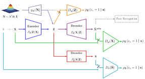
(a)

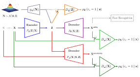
(b)

Figure 6: The training architectures associated with: (a) $\mathsf{DisPF\text{-}MI}$ (P1); (b) $\mathsf{GenPF\text{-}MI}$ (P2).

Learning Procedure: The deep variational PF models $(\textsf{P1})$ (21) and $(\textsf{P2})$ (22) are trained via a six-step alternating block coordinate descent process. In this process, steps 1, 5, and 6 are specific for each model, while steps 2, 3, and 4 are identical for both $(\textsf{P1})$ and $(\textsf{P2})$. Figure 6 illustrates the training architectures for $(\textsf{P1})$ (21) and $(\textsf{P2})$ (22). The training of the DVPF model $(\textsf{P1})$ follows this six-step alternating block coordinate descent process:

(1) Train the Encoder $\bm{\phi}$, Utility Decoder $\bm{\theta}$ and Uncertainty Decoder $\bm{\xi}$.

$$\mathop{\max}_{\bm{\phi},\bm{\theta},\bm{\xi}}\;\mathbb{E}_{P_{\mathsf{D}}(\mathbf{X})}\left[\mathbb{E}_{P_{\bm{\phi}}(\mathbf{Z}\mid\mathbf{X})}\left[\log P_{\bm{\theta}}(\mathbf{X}\!\mid\!\mathbf{Z})\right]\right]-\alpha\;\mathbb{E}_{P_{\mathbf{S},\mathbf{X}}}\left[\mathbb{E}_{P_{\bm{\phi}}\left(\mathbf{Z}\mid\mathbf{X}\right)}\left[\log P_{\bm{\xi}}\left(\mathbf{S}\!\mid\!\mathbf{Z}\right)\right]\right].$$ (24)

(2) Train the Latent Space Discriminator $\bm{\eta}$.

$$\mathop{\min}_{\bm{\eta}}\quad\mathbb{E}_{P_{\mathsf{D}}(\mathbf{X})}\left[\,\mathbb{E}_{P_{\bm{\phi}}(\mathbf{Z}\mid\mathbf{X})}\left[-\log D_{\bm{\eta}}(\mathbf{Z})\right]\,\right]+\mathbb{E}_{Q_{\bm{\psi}}(\mathbf{Z})}\left[\,-\log(1-D_{\bm{\eta}}(\mathbf{Z}))\,\right].$$ (25)

(3) Train the Encoder $\bm{\phi}$ and Prior Distribution Generator $\bm{\psi}$ Adversarially.

$$\mathop{\max}_{\bm{\phi},\bm{\psi}}\quad\mathbb{E}_{P_{\mathsf{D}}(\mathbf{X})}\left[\,\mathbb{E}_{P_{\bm{\phi}}(\mathbf{Z}\mid\mathbf{X})}\left[-\log D_{\bm{\eta}}(\mathbf{Z})\right]\,\right]+\mathbb{E}_{Q_{\bm{\psi}}(\mathbf{Z})}\left[\,-\log(1-D_{\bm{\eta}}(\mathbf{Z}))\,\right].$$ (26)

(4) Train the Utility Output Space Discriminator $\bm{\omega}$.

$$\mathop{\min}_{\bm{\omega}}\quad\mathbb{E}_{P_{\mathsf{D}}(\mathbf{X})}\left[\,-\log D_{\bm{\omega}}(\mathbf{X})\,\right]+\mathbb{E}_{Q_{\bm{\psi}}(\mathbf{Z})}\left[\,-\log\left(1-D_{\bm{\omega}}(\,g_{\bm{\theta}}(\mathbf{Z})\,)\right)\,\right].$$ (27)

(5) Train the Prior Distribution Generator $\bm{\psi}$, Utility Decoder $\bm{\theta}$, and Uncertainty Decoder $\bm{\xi}$ Adversarially.

$$\mathop{\max}_{\bm{\psi},\bm{\theta},\bm{\xi}}\quad\mathbb{E}_{Q_{\bm{\psi}}(\mathbf{Z})}\left[\,-\log\left(1-D_{\bm{\omega}}(\,g_{\bm{\theta}}(\mathbf{Z})\,)\right)\,\right]+\mathbb{E}_{Q_{\bm{\psi}}(\mathbf{Z})}\left[\,-\log\left(1-D_{\bm{\tau}}(\,g_{\bm{\xi}}(\mathbf{Z})\,)\right)\,\right].$$ (28)

(6) Train Uncertainty Output Space (Sensitive Attribute Class) Discriminator $\bm{\tau}$.

$$\mathop{\min}_{\bm{\tau}}\,\mathbb{E}_{P_{\mathbf{S}}}\left[-\log D_{\bm{\tau}}(\mathbf{S})\right]+\mathbb{E}_{Q_{\bm{\psi}}(\mathbf{Z})}\left[-\log\left(1-D_{\bm{\tau}}(g_{\bm{\xi}}(\mathbf{Z}))\right)\right].$$

The DVPF model $(\textsf{P2})$ is trained using alternating block coordinate descent across six steps as follows:

(1) Train the Encoder $\bm{\phi}$, Utility Decoder $\bm{\theta}$ and Uncertainty Decoder $\bm{\varphi}$.

$$\mathop{\max}_{\bm{\phi},\bm{\theta},\bm{\varphi}}\quad\mathbb{E}_{P_{\mathsf{D}}(\mathbf{X})}\left[\mathbb{E}_{P_{\bm{\phi}}(\mathbf{Z}\mid\mathbf{X})}\left[\log P_{\bm{\theta}}(\mathbf{X}\!\mid\!\mathbf{Z})\right]\right]-\alpha\;\;\mathrm{D}_{\mathrm{KL}}\left(P_{\bm{\phi}}(\mathbf{Z}\mid\mathbf{X})\|Q_{\bm{\psi}}(\mathbf{Z})\!\mid\!P_{\mathsf{D}}(\mathbf{X})\right)\\ -\alpha\;\;\mathbb{E}_{P_{\mathbf{S},\mathbf{X}}}\left[\mathbb{E}_{P_{\bm{\phi}}(\mathbf{Z}\mid\mathbf{X})}\left[-\log P_{\bm{\varphi}}(\mathbf{X}\!\mid\!\mathbf{S},\mathbf{Z})\right]\right].$$ (29)

(2) Train the Latent Space Discriminator $\bm{\eta}$.

$$\mathop{\min}_{\bm{\eta}}\quad\mathbb{E}_{P_{\mathsf{D}}(\mathbf{X})}\left[\,\mathbb{E}_{P_{\bm{\phi}}(\mathbf{Z}\mid\mathbf{X})}\left[-\log D_{\bm{\eta}}(\mathbf{Z})\right]\,\right]+\mathbb{E}_{Q_{\bm{\psi}}(\mathbf{Z})}\left[\,-\log(1-D_{\bm{\eta}}(\mathbf{Z}))\,\right].$$ (30)

(3) Train the Encoder $\bm{\phi}$ and Prior Distribution Generator $\bm{\psi}$ Adversarially.

$$\mathop{\max}_{\bm{\phi},\bm{\psi}}\quad\mathbb{E}_{P_{\mathsf{D}}(\mathbf{X})}\left[\,\mathbb{E}_{P_{\bm{\phi}}(\mathbf{Z}\mid\mathbf{X})}\left[-\log D_{\bm{\eta}}(\mathbf{Z})\right]\,\right]+\mathbb{E}_{Q_{\bm{\psi}}(\mathbf{Z})}\left[\,-\log(1-D_{\bm{\eta}}(\mathbf{Z}))\,\right].$$ (31)

(4) Train the Utility Output Space Discriminator $\bm{\omega}$.

$$\mathop{\min}_{\bm{\omega}}\quad\mathbb{E}_{P_{\mathsf{D}}(\mathbf{X})}\left[\,-\log D_{\bm{\omega}}(\mathbf{X})\,\right]+\mathbb{E}_{Q_{\bm{\psi}}(\mathbf{Z})}\left[\,-\log\left(1-D_{\bm{\omega}}(\,g_{\bm{\theta}}(\mathbf{Z})\,)\right)\,\right].$$ (32)

(5) Train the Prior Distribution Generator $\bm{\psi}$, Utility Decoder $\bm{\theta}$, and Uncertainty Decoder $\bm{\varphi}$ Adversarially.

$$\mathop{\max}_{\bm{\psi},\bm{\theta},\bm{\varphi}}\quad\mathbb{E}_{Q_{\bm{\psi}}(\mathbf{Z})}\left[\,-\log\left(1-D_{\bm{\omega}}(\,g_{\bm{\theta}}(\mathbf{Z})\,)\right)\,\right]+\mathbb{E}_{Q_{\bm{\psi}}(\mathbf{Z})}\left[\,-\log\left(1-D_{\bm{\omega}}(\,g_{\bm{\varphi}}(\mathbf{S},\mathbf{Z})\,)\right)\,\right].$$ (33)

(6) Train the Uncertainty Output Space Discriminator $\bm{\omega}$.

$$\mathop{\min}_{\bm{\omega}}\quad\mathbb{E}_{P_{\mathsf{D}}(\mathbf{X})}\left[\,-\log D_{\bm{\omega}}(\mathbf{X})\,\right]+\mathbb{E}_{Q_{\bm{\psi}}(\mathbf{Z})}\left[\,-\log\left(1-D_{\bm{\omega}}(\,g_{\bm{\varphi}}(\mathbf{S},\mathbf{Z})\,)\right)\,\right].$$ (34)

The detailed training algorithms of these models are shown in Algorithm 1 and Algorithm 2.

1:Input: Training Dataset: $\{\left(\mathbf{s}_{n},\mathbf{x}_{n}\right)\}_{n=1}^{N}$; Hyper-Parameter: $\alpha$

2:$\bm{\phi},\bm{\theta},\bm{\psi},\bm{\varphi},\bm{\eta},\bm{\omega}\;\leftarrow$ Initialize Network Parameters

3:repeat(1) Train the Encoder $\bm{\phi}$, Utility Decoder $\bm{\theta}$, Uncertainty Decoder $\bm{\xi}$

4:      Sample a mini-batch $\{\mathbf{x}_{m},\mathbf{s}_{m}\}_{m=1}^{M}\sim P_{\mathsf{D}}(\mathbf{X})P_{\mathbf{S}\mid\mathbf{X}}$

5:      Compute encoder outputs $\bm{\mu}_{m}^{\mathsf{enc}},\bm{\sigma}_{m}^{\mathsf{enc}}=f_{\bm{\phi}}(\mathbf{x}_{m}),\forall m\in[M]$

6:      Apply reparametrization trick $\mathbf{z}_{m}^{\mathsf{enc}}=\bm{\mu}_{m}^{\mathsf{enc}}+\bm{\epsilon}_{m}\odot\bm{\sigma}_{m}^{\mathsf{enc}},\;\bm{\epsilon}_{m}\sim\mathcal{N}(0,\mathbf{I}),\;\forall m\in[M]$

7:      Sample $\{\mathbf{n}_{m}\}_{m=1}^{M}\sim\mathcal{N}(\bm{0},\mathbf{I})$

8:      Compute $\bm{\mu}_{m}^{\mathsf{prior}},\bm{\sigma}_{m}^{\mathsf{prior}}=g_{\bm{\psi}}(\mathbf{n}_{m}),\forall m\in[M]$

9:      Compute $\mathbf{z}_{m}^{\mathsf{prior}}\!\!=\!\bm{\mu}_{m}^{\mathsf{prior}}\!+\bm{\epsilon}_{m}^{\prime}\odot\bm{\sigma}_{m}^{\mathsf{prior}},\bm{\epsilon}_{m}^{\prime}\!\sim\!\mathcal{N}(0,\mathbf{I}),\forall m\!\in\![M]\!$

10:      Compute $\mathbf{\widehat{x}}_{m}=g_{\bm{\theta}}(\mathbf{z}_{m}^{\mathsf{enc}}),\forall m\in[M]$

11:      Compute $\mathbf{\widehat{s}}_{m}=g_{\bm{\xi}}(\mathbf{z}_{m}^{\mathsf{enc}}),\forall m\in[M]$

12:      Back-propagate loss:

$$\quad\mathcal{L}\left(\bm{\phi},\bm{\theta},\bm{\xi}\right)=\!-\frac{1}{M}\sum_{m=1}^{M}\!\Big{(}\mathsf{dis}(\mathbf{x}_{m},\mathbf{\widehat{x}}_{m})-\,\alpha\;\log P_{\bm{\xi}}(\mathbf{s}_{m}\!\mid\!\mathbf{z}_{m}^{\mathsf{enc}})\Big{)}$$

(2) Train the Latent Space Discriminator $\bm{\eta}$

13:      Sample $\{\mathbf{x}_{m}\}_{m=1}^{M}\sim P_{\mathsf{D}}(\mathbf{X})$

14:      Sample $\{\mathbf{n}_{m}\}_{m=1}^{M}\sim\mathcal{N}(\bm{0},\mathbf{I})$

15:      Compute $\mathbf{z}_{m}^{\mathsf{enc}}\!$ from $\!f_{\!\bm{\phi}}(\mathbf{x}_{m})\!$ with reparametrization, $\forall m\!\in\![M]\!$

16:      Compute $\mathbf{z}_{m}^{\mathsf{prior}}\!\!$ from $\!g_{\bm{\psi}}(\mathbf{n}_{m}\!)\!$ with reparametrization, $\!\forall m\!\in\![M]\!$

17:      Back-propagate loss:

$$\;\;\;\mathcal{L}\left(\bm{\eta}\right)=-\frac{\alpha}{M}\;\sum_{m=1}^{M}\log D_{\bm{\eta}}(\mathbf{z}_{m}^{\mathsf{enc}})+\log\big{(}1-D_{\bm{\eta}}(\,\mathbf{z}_{m}^{\mathsf{prior}}\,)\big{)}$$

(3) Train the Encoder $\bm{\phi}$ and Prior Distribution Generator $\bm{\psi}$ Adversarially

18:      Sample $\{\mathbf{x}_{m}\}_{m=1}^{M}\sim P_{\mathsf{D}}(\mathbf{X})$

19:      Compute $\mathbf{z}_{m}^{\mathsf{enc}}\!$ from $\!f_{\!\bm{\phi}}(\mathbf{x}_{m})\!$ with reparametrization, $\forall m\!\in\![M]$

20:      Sample $\{\mathbf{n}_{m}\}_{m=1}^{M}\sim\mathcal{N}(\bm{0},\mathbf{I})$

21:      Compute $\mathbf{z}_{m}^{\mathsf{prior}}\!\!$ from $\!g_{\bm{\psi}}(\mathbf{n}_{m}\!)\!$ with reparametrization, $\!\forall m\!\in\![M]\!$

22:      Back-propagate loss:

$$\;\;\;\mathcal{L}\left(\bm{\phi},\bm{\psi}\right)=\frac{\alpha}{M}\;\sum_{m=1}^{M}\log D_{\bm{\eta}}(\mathbf{z}_{m}^{\mathsf{enc}})+\log\big{(}1-D_{\bm{\eta}}(\,\mathbf{z}_{m}^{\mathsf{prior}}\,)\big{)}$$

(4) Train the Utility Output Space Discriminator $\bm{\omega}$

23:      Sample $\{\mathbf{x}_{m}\}_{m=1}^{M}\sim P_{\mathsf{D}}(\mathbf{X})$

24:      Sample $\{\mathbf{n}_{m}\}_{m=1}^{M}\sim\mathcal{N}\!\left(\bm{0},\mathbf{I}\right)$

25:      Compute $\mathbf{z}_{m}^{\mathsf{prior}}\!\!$ from $\!g_{\bm{\psi}}(\mathbf{n}_{m}\!)\!$ with reparametrization, $\!\forall m\!\in\![M]\!$

26:      Compute $\mathbf{\widehat{x}}_{m}=g_{\bm{\theta}}(\mathbf{z}_{m}^{\mathsf{prior}}),\forall m\in[M]$

27:      Back-propagate loss:

$$\mathcal{L}\left(\bm{\omega}\right)=-\frac{1}{M}\sum_{m=1}^{M}\log D_{\bm{\omega}}(\mathbf{x}_{m})+\log\left(1-D_{\bm{\omega}}(\,\mathbf{\widehat{x}}_{m}\,)\right)$$

(5) Train the Prior Distribution Generator $\bm{\psi}$, Utility Decoder $\bm{\theta}$, and Uncertainty Decoder $\bm{\xi}$ Adversarially

28:      Sample $\{\mathbf{n}_{m}\}_{m=1}^{M}\sim\mathcal{N}\!\left(\bm{0},\mathbf{I}\right)$

29:      Compute $\mathbf{z}_{m}^{\mathsf{prior}}\!\!$ from $\!g_{\bm{\psi}}(\mathbf{n}_{m}\!)\!$ with reparametrization, $\!\forall m\!\in\![M]\!$

30:      Compute $\mathbf{\widehat{x}}_{m}=g_{\bm{\theta}}\left(\mathbf{z}_{m}^{\mathsf{prior}}\right),\forall m\in[M]$

31:      Compute $\mathbf{\widehat{s}}_{m}=g_{\bm{\xi}}\left(\mathbf{z}_{m}^{\mathsf{prior}}\right),\forall m\in[M]$

32:      Back-propagate loss:

$$\;\;\;\;\mathcal{L}\left(\bm{\psi},\bm{\theta},\bm{\xi}\right)\!=\!\frac{1}{M}\!\!\sum_{m=1}^{M}\!\!\log\left(1\!-\!D_{\bm{\omega}}(\,\mathbf{\widehat{x}}_{m}\,)\right)+\log\left(1\!-\!D_{\bm{\tau}}(\,\mathbf{\widehat{s}}_{m}\,)\right)\!\!\!\!$$

(6) Train Uncertainty Output Space Discriminator $\bm{\omega}$

33:      Sample a mini-batch $\{\mathbf{s}_{m},\mathbf{x}_{m}\}_{m=1}^{M}\sim P_{\mathsf{D}}(\mathbf{X})P_{\mathbf{S}\mid\mathbf{X}}$

34:      Sample $\{\mathbf{n}_{m}\}_{m=1}^{M}\sim\mathcal{N}(\bm{0},\mathbf{I})$

35:      Compute $\mathbf{z}_{m}^{\mathsf{prior}}\!\!$ from $\!g_{\bm{\psi}}(\mathbf{n}_{m}\!)\!$ with reparametrization, $\!\forall m\!\in\![M]\!$

36:      Compute $\mathbf{\widehat{s}}_{m}\sim g_{\bm{\xi}}\left(\mathbf{z}_{m}^{\mathsf{prior}}\right),\forall m\in[M]$

37:      Back-propagate loss:

$$\mathcal{L}\left(\bm{\tau}\right)=\frac{1}{M}\sum_{m=1}^{M}\log D_{\bm{\tau}}(\,\mathbf{s}_{m}\,)+\log\left(1-D_{\bm{\tau}}(\,\mathbf{\widehat{s}}_{m}\,)\right)$$

38:until Convergence

39:return $\bm{\phi},\bm{\theta},\bm{\psi},\bm{\varphi},\bm{\eta},\bm{\omega}$

Algorithm 1 Deep Variational $\mathsf{DisPF}$ training algorithm associated with $\textsf{DisPF\text{-}MI}\;(\textsf{P1})$

1:Input: Training Dataset: $\{\left(\mathbf{s}_{n},\mathbf{x}_{n}\right)\}_{n=1}^{N}$; Hyper-Parameter: $\alpha$

2:$\bm{\phi},\bm{\theta},\bm{\psi},\bm{\varphi},\bm{\eta},\bm{\omega}\;\leftarrow$ Initialize Network Parameters

3:repeat(1) Train the Encoder $\bm{\phi}$, Utility Decoder $\bm{\theta}$, Uncertainty Decoder $\bm{\varphi}$

4:      Sample a mini-batch $\{\mathbf{x}_{m},\mathbf{s}_{m}\}_{m=1}^{M}\sim P_{\mathsf{D}}(\mathbf{X})P_{\mathbf{S}\mid\mathbf{X}}$

5:      Compute encoder outputs $\bm{\mu}_{m}^{\mathsf{enc}},\bm{\sigma}_{m}^{\mathsf{enc}}=f_{\bm{\phi}}(\mathbf{x}_{m}),\forall m\in[M]$

6:      Apply reparametrization trick $\mathbf{z}_{m}^{\mathsf{enc}}=\bm{\mu}_{m}^{\mathsf{enc}}+\bm{\epsilon}_{m}\odot\bm{\sigma}_{m}^{\mathsf{enc}},\;\bm{\epsilon}_{m}\sim\mathcal{N}(0,\mathbf{I}),\;\forall m\in[M]$

7:      Sample $\{\mathbf{n}_{m}\}_{m=1}^{M}\sim\mathcal{N}(\bm{0},\mathbf{I})$

8:      Compute $\bm{\mu}_{m}^{\mathsf{prior}},\bm{\sigma}_{m}^{\mathsf{prior}}=g_{\bm{\psi}}(\mathbf{n}_{m}),\forall m\in[M]$

9:      Compute $\mathbf{z}_{m}^{\mathsf{prior}}\!\!=\!\bm{\mu}_{m}^{\mathsf{prior}}\!+\bm{\epsilon}_{m}^{\prime}\odot\bm{\sigma}_{m}^{\mathsf{prior}},\bm{\epsilon}_{m}^{\prime}\!\sim\!\mathcal{N}(0,\mathbf{I}),\forall m\!\in\![M]\!$

10:      Compute $\mathbf{\widehat{x}}_{m}=g_{\bm{\theta}}(\mathbf{z}_{m}^{\mathsf{enc}}),\forall m\in[M]$

11:      Compute $\mathbf{\widetilde{x}}_{m}=g_{\bm{\varphi}}(\mathbf{z}_{m}^{\mathsf{enc}},\mathbf{s}_{m}),\forall m\in[M]$

12:      Back-propagate loss:

$$\quad\mathcal{L}\left(\bm{\phi},\bm{\theta},\bm{\varphi}\right)=\!-\frac{1}{M}\sum_{m=1}^{M}\!\Big{(}\mathsf{dis}(\mathbf{x}_{m},\mathbf{\widehat{x}}_{m})-\alpha\,\mathrm{D}_{\mathrm{KL}}\!\left(P_{\bm{\phi}}(\mathbf{z}_{m}^{\mathsf{enc}}\!\mid\!\mathbf{x}_{m})\|Q_{\bm{\psi}}(\mathbf{z}_{m}^{\mathsf{prior}})\right)+\,\alpha\,\mathsf{dis}(\mathbf{x}_{m},\mathbf{\widetilde{x}}_{m})\Big{)}$$ (35)

(2) Train the Latent Space Discriminator $\bm{\eta}$

13:      Sample $\{\mathbf{x}_{m}\}_{m=1}^{M}\sim P_{\mathsf{D}}(\mathbf{X})$

14:      Sample $\{\mathbf{n}_{m}\}_{m=1}^{M}\sim\mathcal{N}(\bm{0},\mathbf{I})$

15:      Compute $\mathbf{z}_{m}^{\mathsf{enc}}\!$ from $\!f_{\!\bm{\phi}}(\mathbf{x}_{m})\!$ with reparametrization, $\forall m\!\in\![M]\!$

16:      Compute $\mathbf{z}_{m}^{\mathsf{prior}}\!\!$ from $\!g_{\bm{\psi}}(\mathbf{n}_{m}\!)\!$ with reparametrization, $\!\forall m\!\in\![M]\!$

17:      Back-propagate loss:

$$\;\;\;\mathcal{L}\left(\bm{\eta}\right)=-\frac{\alpha}{M}\;\sum_{m=1}^{M}\log D_{\bm{\eta}}(\mathbf{z}_{m}^{\mathsf{enc}})+\log\big{(}1-D_{\bm{\eta}}(\,\mathbf{z}_{m}^{\mathsf{prior}}\,)\big{)}$$

(3) Train the Encoder $\bm{\phi}$ and Prior Distribution Generator $\bm{\psi}$ Adversarially

18:      Sample $\{\mathbf{x}_{m}\}_{m=1}^{M}\sim P_{\mathsf{D}}(\mathbf{X})$

19:      Compute $\mathbf{z}_{m}^{\mathsf{enc}}\!$ from $\!f_{\!\bm{\phi}}(\mathbf{x}_{m})\!$ with reparametrization, $\forall m\!\in\![M]$

20:      Sample $\{\mathbf{n}_{m}\}_{m=1}^{M}\sim\mathcal{N}(\bm{0},\mathbf{I})$

21:      Compute $\mathbf{z}_{m}^{\mathsf{prior}}\!\!$ from $\!g_{\bm{\psi}}(\mathbf{n}_{m}\!)\!$ with reparametrization, $\!\forall m\!\in\![M]\!$

22:      Back-propagate loss:

$$\;\;\;\mathcal{L}\left(\bm{\phi},\bm{\psi}\right)=\frac{\alpha}{M}\;\sum_{m=1}^{M}\log D_{\bm{\eta}}(\mathbf{z}_{m}^{\mathsf{enc}})+\log\big{(}1-D_{\bm{\eta}}(\,\mathbf{z}_{m}^{\mathsf{prior}}\,)\big{)}$$

(4) Train the Utility Output Space Discriminator $\bm{\omega}$

23:      Sample $\{\mathbf{x}_{m}\}_{m=1}^{M}\sim P_{\mathsf{D}}(\mathbf{X})$

24:      Sample $\{\mathbf{n}_{m}\}_{m=1}^{M}\sim\mathcal{N}\!\left(\bm{0},\mathbf{I}\right)$

25:      Compute $\mathbf{z}_{m}^{\mathsf{prior}}\!\!$ from $\!g_{\bm{\psi}}(\mathbf{n}_{m}\!)\!$ with reparametrization, $\!\forall m\!\in\![M]\!$

26:      Compute $\mathbf{\widehat{x}}_{m}=g_{\bm{\theta}}(\mathbf{z}_{m}^{\mathsf{prior}}),\forall m\in[M]$

27:      Back-propagate loss:

$$\mathcal{L}\left(\bm{\omega}\right)=-\frac{1}{M}\sum_{m=1}^{M}\log D_{\bm{\omega}}(\mathbf{x}_{m})+\log\left(1-D_{\bm{\omega}}(\,\mathbf{\widehat{x}}_{m}\,)\right)$$

(5) Train the Prior Distribution Generator $\bm{\psi}$, Utility Decoder $\bm{\theta}$, and Uncertainty Decoder $\bm{\varphi}$ Adversarially

28:      Sample $\{\mathbf{n}_{m}\}_{m=1}^{M}\sim\mathcal{N}\!\left(\bm{0},\mathbf{I}\right)$

29:      Compute $\mathbf{z}_{m}^{\mathsf{prior}}\!\!$ from $\!g_{\bm{\psi}}(\mathbf{n}_{m}\!)\!$ with reparametrization, $\!\forall m\!\in\![M]\!$

30:      Compute $\mathbf{\widehat{x}}_{m}\sim g_{\bm{\theta}}\left(\mathbf{z}_{m}^{\mathsf{prior}}\right),\forall m\in[M]$

31:      Compute $\mathbf{\widetilde{x}}_{m}\sim g_{\bm{\varphi}}\left(\mathbf{z}_{m}^{\mathsf{prior}},\mathbf{s}_{m}\right),\forall m\in[M]$

32:      Back-propagate loss:

$$\;\;\;\;\mathcal{L}\left(\bm{\psi},\bm{\theta},\bm{\varphi}\right)\!=\!\frac{1}{M}\!\!\sum_{m=1}^{M}\!\!\log\left(1\!-\!D_{\bm{\omega}}(\,\mathbf{\widehat{x}}_{m}\,)\right)+\log\left(1\!-\!D_{\bm{\omega}}(\,\mathbf{\widetilde{x}}_{m}\,)\right)\!\!\!\!$$

(6) Train Uncertainty Output Space Discriminator $\bm{\omega}$

33:      Sample a mini-batch $\{\mathbf{s}_{m},\mathbf{x}_{m}\}_{m=1}^{M}\sim P_{\mathsf{D}}(\mathbf{X})P_{\mathbf{S}\mid\mathbf{X}}$

34:      Sample $\{\mathbf{n}_{m}\}_{m=1}^{M}\sim\mathcal{N}(\bm{0},\mathbf{I})$

35:      Compute $\mathbf{z}_{m}^{\mathsf{prior}}\!\!$ from $\!g_{\bm{\psi}}(\mathbf{n}_{m}\!)\!$ with reparametrization, $\!\forall m\!\in\![M]\!$

36:      Compute $\mathbf{\widetilde{x}}_{m}\sim g_{\bm{\varphi}}\left(\mathbf{z}_{m}^{\mathsf{prior}},\mathbf{s}_{m}\right),\forall m\in[M]$

37:      Back-propagate loss:

$$\mathcal{L}\left(\bm{\omega}\right)=\frac{1}{M}\sum_{m=1}^{M}\log D_{\bm{\omega}}(\,\mathbf{x}_{m}\,)+\log\left(1-D_{\bm{\omega}}(\,\mathbf{\widetilde{x}}_{m}\,)\right)$$

38:until Convergence

39:return $\bm{\phi},\bm{\theta},\bm{\psi},\bm{\varphi},\bm{\eta},\bm{\omega}$

Algorithm 2 Deep Variational $\mathsf{GenPF}$ training algorithm associated with $\mathsf{GenPF\text{-}MI}\;(\textsf{P2})$

5.5 Role of Information Complexity in Privacy Leakage

The implicit assumption in the PF model is to have pre-defined interests in the game between the ‘defender’ (data owner/user) and the ‘adversary’; that is, the data owner knows in advance what feature/variable of the underlying data the adversary is interested in. Accordingly, the data release mechanism can be optimized/tuned to minimize any inference the adversary can make about this specific random variable. However, this assumption may be violated in most real-world scenarios. The attribute that the defender may assume as sensitive may not be the attribute of interest for the inferential adversary. As an example, for a given utility task at hand, the defender may try to restrict inference on gender recognition while the adversary is interested in inferring an individual’s identity or facial emotion. Inspired by (Issa et al., 2019), and in contrast to the above setups, we consider the scenario in which the adversary is curious about an attribute that is unknown to the system designer. In (Atashin et al., 2021), we assumed the adversary is interested in an attribute $\mathbf{S}$ of data $\mathbf{X}$ which is not known a priori to the defender. Next, we argued that the information complexity of the representation measured by mutual information $\mathrm{I}\left(\mathbf{X};\mathbf{Z}\right)$ can also limit the information leakage about the unknown sensitive variable.

6 Face Recognition Experiments

Face recognition systems represent a crucial segment within the larger domain of biometric technology. They operate by identifying or verifying a person’s identity through the analysis of facial features in digital images or video frames. The technology employs complex algorithms and machine learning models to compare specific facial attributes in an input image with those in a known database, thereby establishing an individual’s identity or lack thereof. Face recognition systems find widespread applications, ranging from security and surveillance to social media and smartphone technology.

6.1 Face Recognition Leading Models and Their Core Mechanisms

The evolution of face recognition technology has been significantly influenced by the development of several groundbreaking models, each distinguished by its unique features and mechanisms. Prominent among these are DeepFace (Taigman et al., 2014), FaceNet (Schroff et al., 2015), OpenFace (Amos et al., 2016), SphereFace (Liu et al., 2017), CosFace (Wang et al., 2018), ArcFace (Deng et al., 2019a), and AdaFace (Kim et al., 2022). These models have advanced the field through their innovative use of deep learning techniques, setting new standards in accuracy and reliability for face recognition tasks.

DeepFace, developed by Facebook, employs a deep neural network with over 120 million parameters, demonstrating notable robustness against pose variations through advanced 3D modeling techniques. FaceNet, from Google, uses a ‘triplet loss’ function to optimize distances between anchor, positive, and negative images. Despite its effectiveness, FaceNet faces challenges related to the large number of triplets in extensive datasets and complexities in mining semi-hard samples. OpenFace, a Carnegie Mellon University innovation, offers a lightweight yet efficient alternative, focusing on ‘TripletHardLoss’ for challenging sample selection during training. This model excels in environments with limited computational resources. Subsequent to OpenFace, SphereFace introduced an angular margin penalty in its loss function to enhance intra-class compactness and inter-class separation. SphereFace, however, encountered training stability challenges due to the need for computational approximations in its loss function. Building on these advancements, CosFace added a cosine margin penalty directly to the target logit, simplifying the implementation and improving performance without requiring joint supervision from the softmax loss. This marked a significant step forward in the development of margin-based loss functions. ArcFace, from InsightFace, further refined the approach by introducing an ’Additive Angular Margin Loss’, which optimizes the geodesic distance margin on a normalized hypersphere. Known for its ease of implementation and computational efficiency, ArcFace achieved state-of-the-art performance across various benchmarks. Most recently, AdaFace has represented a significant leap in addressing image quality variations in face recognition. By correlating feature norms with image quality, AdaFace adapts its margin function to emphasize hard samples in high-quality images and de-emphasize them in lower-quality ones. This adaptive approach, blending angular and additive margins based on image quality, represents a notable advancement in the field.

6.2 Backbone Architectures for Feature Extraction

In the context of face recognition systems, backbone architectures provide the core structure essential for extracting and learning high-level features from raw input data. These architectures, underpinning the design of face recognition models, significantly influence their capacity to discern facial features and, consequently, their performance. One of the key architectures in this domain is the Improved ResNet, or iResNet (Duta et al., 2021). As an advanced iteration of the ResNet (He et al., 2016) model, iResNet integrates modifications that aim to resolve issues related to the degradation of deeper networks. It is characterized by its residual learning framework, which effectively tackles the vanishing gradient problem, a common challenge with deep neural networks. This allows for the training of networks with increased depth, thereby facilitating a more profound extraction of facial features. The modularity of iResNet, which can be adapted to various depths, provides the flexibility to balance computational efficiency and model accuracy based on the specific requirements of a given task. This adaptability extends the use of iResNet across different face recognition models, each leveraging the architecture’s strengths according to their individual design principles. Other backbone architectures, such as VGGNet (Simonyan and Zisserman, 2014) and MobileNet (Howard et al., 2017), are also employed in the design of face recognition models. VGGNet, with its homogeneously stacked convolutional layers, excels in extracting features from input images of varying complexity. On the other hand, MobileNet, with its depthwise separable convolutions, offers an efficient, lightweight solution optimal for mobile and edge computing applications. The choice of backbone architecture significantly influences the face recognition model’s performance, shaping its ability to extract necessary features, adapt to varying task complexities, and function efficiently within the given computational constraints. As such, selecting the most suitable architecture is crucial for the successful deployment of a face recognition system.

6.3 Datasets for Training and Validation

The viability and robustness of face recognition systems hinge significantly on the quality and diversity of the datasets used for their training and validation. These datasets supply a spectrum of facial data crucial for model training, acting as the cornerstone upon which these systems develop their ability to recognize and differentiate facial features.

The MSCeleb1M dataset (Deng et al., 2019b) is a noteworthy resource in this domain, providing a comprehensive collection of over a million celebrity images. Its richness in terms of varied expressions, poses, illumination conditions, and occlusions makes it invaluable for model training, enhancing the system’s capacity to handle real-world variability.

The WebFace dataset (Zhu et al., 2021), officially known as CASIA-WebFace, provides a large-scale face dataset for training deep models. With nearly half a million images from over 10,000 individuals, it offers a diverse range of facial images sourced from the internet. This dataset has become a staple in the face recognition community for developing and benchmarking algorithms, particularly because of its real-world diversity and the challenges it presents in terms of data variability.

The MORPH dataset (Ricanek and Tesafaye, 2006) distinguishes itself with its focus on longitudinal facial data, charting the progression of facial features over time. The inclusion of aging-related variations makes this dataset crucial for the development of age-invariant face recognition capabilities, an essential attribute for models deployed in dynamic, real-world scenarios.

The FairFace dataset (Karkkainen and Joo, 2021) is an intervention in the realm of equitable face recognition. Designed to mitigate racial and demographic biases, it includes a balanced representation of seven racial groups and a diverse distribution of age and gender within each group. With approximately 100,000 (exactly 108,501) images, FairFace is a valuable resource for training and evaluating face recognition systems, ensuring they perform fairly across different demographics. This dataset is particularly crucial for developing models that can operate justly in multicultural societies, where fairness and inclusivity are paramount.

For unconstrained face recognition, the Labeled Faces in the Wild (LFW) (Huang et al., 2008) and the IARPA Janus Benchmark-C (IJBC) (Maze et al., 2018) datasets have made significant contributions. The LFW dataset comprises images collected from the internet, encapsulating the real-world conditions a face recognition system is likely to encounter, including variability in pose, lighting, and expression. IJBC, on the other hand, provides a challenging, large-scale evaluation of face recognition technology under uncontrolled conditions. It includes several variations such as pose, illumination, expression, race, and age, thereby pushing the boundaries of model performance.

6.4 Metrics Used to Evaluate Face Recognition Model Performance

In this subsection, we will elucidate the key metrics utilized to assess the performance of face recognition models in our experiments. This elucidation may prove particularly helpful to readers who lack prior familiarity with the components of biometric systems or the interpretation of fundamental information-theoretic measures. Readers with existing knowledge in these areas may choose to bypass this introductory material.

6.4.1 False Match Rate ($\mathsf{FMR}$)

The False Match Rate ($\mathsf{FMR}$), also known as the False Acceptance Rate ($\mathsf{FAR}$), quantifies the rate at which the system erroneously accepts an imposter’s face as a genuine match. In other words, it measures the probability of a false positive identification. $\mathsf{FMR}$ is calculated by dividing the number of falsely accepted imposter faces by the total number of verification attempts on imposter faces.

$$\mathsf{FMR}=\frac{\mathsf{Number~{}of~{}False~{}Acceptances}}{\mathsf{Total~{}Imposter~{}Verification~{}Attempts}}.$$ (36)

Lower $\mathsf{FMR}$ values indicate a higher level of security and a reduced likelihood of unauthorized access. The choice of an appropriate threshold for $\mathsf{FMR}$ is essential and often depends on the specific application and security requirements. A lower threshold increases security but may lead to higher False Rejection Rates ($\mathsf{FRR}$), which can inconvenience legitimate users.

6.4.2 True Match Rate ($\mathsf{TMR}$)

The True Match Rate ($\mathsf{TMR}$), also known as the True Acceptance Rate (TAR), measures the system’s ability to correctly identify or verify genuine matches. It quantifies the probability of a true positive identification, where the system correctly accepts a genuine user. $\mathsf{TMR}$ is calculated by dividing the number of correctly accepted genuine matches by the total number of verification attempts on genuine faces.

$$\mathsf{TMR}=\frac{\mathsf{Number~{}of~{}True~{}Acceptances}}{\mathsf{Total~{}Genuine~{}Verification~{}Attempts}}.$$ (37)

Higher $\mathsf{TMR}$ values signify a higher level of accuracy in correctly accepting genuine users, which is desirable in most face recognition applications. However, a high $\mathsf{TMR}$ may be accompanied by an increased risk of false positives (higher $\mathsf{FMR}$) if the threshold is set too low. Balancing $\mathsf{TMR}$ and $\mathsf{FMR}$ is crucial to achieve the desired level of security and convenience in the application.

6.4.3 Accuracy ($\mathsf{Acc}$)

Accuracy is a fundamental metric that provides a holistic view of a face recognition system’s performance. It encompasses both the $\mathsf{TMR}$ and the $\mathsf{FMR}$ by considering the correct and incorrect identifications collectively. Accuracy is calculated by dividing the total number of correct verifications (true positives and true negatives) by the total number of verification attempts (all cases).

$$\mathsf{Acc}=\frac{\mathsf{Number~{}of~{}True~{}Positives}+\mathsf{Number~{}of~{}True~{}Negatives}}{\mathsf{Total~{}Verification~{}Attempts}}.$$ (38)

High accuracy values indicate a robust system with a low rate of both false positives and false negatives. Achieving a high accuracy rate is typically the primary objective in face recognition applications, as it ensures that the system correctly identifies genuine users while minimizing the likelihood of unauthorized access.

6.4.4 Shannon Entropy

Entropy is a measure of the randomness or uncertainty of a variable. For a discrete variable $\mathbf{S}$ with a probability mass function $P_{\mathbf{S}}$, the Shannon entropy is defined as $\mathrm{H}(\mathbf{S})=-\sum P_{\mathbf{S}}\log(P_{\mathbf{S}})$. Entropy enables us to assess the degree of uncertainty within our (sensitive) labels $\mathbf{S}$. The maximum possible entropy of a discrete random variable is $\log\left(|\mathcal{S}|\right)$, where $|\mathcal{S}|$ represents the cardinality of the variable. For example, if $\mathbf{S}$ represents gender (with two categories), the maximum entropy is $\log_{2}(2)=1$, while for race (e.g. with four categories), the maximum entropy is $\log_{2}(4)=2$. When our calculated entropy is less than the maximum value of $\log\left(|\mathcal{S}|\right)$, it indicates an imbalance in the distribution of our labels. In other words, the labels are not uniformly distributed, and there is some degree of predictability or bias in the variable.

6.4.5 Mutual Information

Mutual information quantifies the extent to which knowledge of one variable reduces uncertainty about another. It is defined as $\mathrm{I}\left(\mathbf{S};\mathbf{Z}\right)=\mathrm{H}\left(\mathbf{S}\right)-\mathrm{H}\left(\mathbf{S}\mid|\mathbf{Z}\right)$. This formula measures the reduction in uncertainty about the (sensitive) labels ($\mathbf{S}$) when we possess knowledge of the embeddings ($\mathbf{Z}$). The close proximity of the values of $\mathrm{I}\left(\mathbf{S};\mathbf{Z}\right)$ to $\mathrm{H}(\mathbf{S})$ indicates that knowing the embeddings $\mathbf{Z}$ significantly reduces uncertainty about the labels $\mathbf{S}$. Mutual information is a symmetric measure ($\mathrm{I}\left(\mathbf{S};\mathbf{Z}\right)=\mathrm{I}\left(\mathbf{Z};\mathbf{S}\right)$). Additionally, it can be expressed as $\mathrm{I}\left(\mathbf{S};\mathbf{Z}\right)=\mathrm{H}(\mathbf{S})+\mathrm{H}(\mathbf{Z})-\mathrm{H}(\mathbf{S},\mathbf{Z})$, where $\mathrm{H}(\mathbf{S},\mathbf{Z})$ represents the joint entropy of both $\mathbf{S}$ and $\mathbf{Z}$. This equation reveals that mutual information also quantifies the reduction in joint uncertainty regarding both $\mathbf{S}$ and $\mathbf{Z}$ when we have information about either variable. It is essential to emphasize that $\mathrm{I}\left(\mathbf{S};\mathbf{Z}\right)\leq\min\left(\mathrm{H}(\mathbf{S}),\mathrm{H}(\mathbf{Z})\right)$. This inequality stems from the fact that information shared between $\mathbf{S}$ and $\mathbf{Z}$ cannot exceed the initial uncertainty present in either $\mathbf{S}$ or $\mathbf{Z}$. In simpler terms, mutual information cannot exceed the total information content in either $\mathbf{S}$ or $\mathbf{Z}$.

6.5 Experiments Setup

We consider the state-of-the-art Face Recognition (FR) backbones with three variants of iResNet (He et al., 2016; Deng et al., 2019a) architecture (iResNet100, iResNet50, and iResNet18). These architectures have been trained using either the MS1MV3 (Deng et al., 2019b) or WebFace4M/12M (Zhu et al., 2021) datasets. For loss functions, ArcFace (Deng et al., 2019a) and AdaFace (Kim et al., 2022) methods were employed. For the training phase, we utilized pre-trained models sourced from the aforementioned studies. All input images underwent a standardized pre-processing routine, encompassing alignment, scaling, and normalization. This was in accordance with the specifications of the pre-trained models. We then trained our networks using the Morph dataset (Ricanek and Tesafaye, 2006) and FairFace (Karkkainen and Joo, 2021), focusing on different demographic group combinations such as race and gender. Figure 7 depicts our framework during the training phase for a specific setup, which we will explain later. Figure 8 shows the trained modules. Figure 9 illustrates our framework during the inference phase. We will provide more details in Sec. 6.6.

6.5.1 Learning Scenarios

We consider two types of data available for $\mathbf{X}$: (i) raw image samples, and (ii) feature extractions, commonly referred to as embeddings, from the facial images. In the case of raw images, we have the option to employ one of two distinct encoder types: (i) a custom encoder, which will be trained from scratch, or (ii) a backbone encoder that leverages a pre-trained network and undergoes further refinement via fine-tuning during the training process. Alternatively, when working with facial image embeddings, we utilize a custom multi-layer perceptron (MLP) encoder, which is also intended to be trained from scratch. Based on the utility and uncertainty decoder objectives, we identify two types of decoder tasks: (i) reconstruction, and (ii) classification tasks. Taking these setups into account, we investigate three learning scenarios as follows:

End-to-End Raw Data Scratch Learning: In this approach, our objective is to train a custom encoder model (alongside other networks) from scratch, using raw data samples as input. The model learns data representations directly from the raw input without relying on prior knowledge from a pre-trained model. This method is suitable when the dataset is sufficiently large and diverse to support training a deep neural network from scratch and when the aim is to learn data representations directly from the raw input.

Raw Data Transfer Learning with Fine-Tuning: In this approach, a pre-trained (base) model is employed to enhance the performance of a model on a potentially smaller or more specialized dataset. The pre-trained model serves as the backbone, with a mid-layer selected as the latent representation. This method is suitable when the dataset is small and specialized, and fine-tuning the pre-trained model can offer significant improvement over training a model from scratch.

Embedding-Based Data Learning: In this approach, our goal is to employ a multi-layer perceptron (MLP) projector network as our encoder model, which uses extracted features (embeddings) as input. This method is suitable when a fine-tuned face recognition model has already learned meaningful (useful) features from a large and diverse dataset. Utilizing these features as input to a machine learning model can potentially offer an improvement over training a model from scratch or fine-tuning a pre-trained model. This approach leverages the pre-trained model’s ability to capture relevant information and may reduce the computational cost and complexity associated with end-to-end learning from raw data. Figure 7 depicts an example of our training framework for this setup.

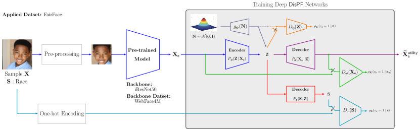
Figure 7: Training the deep variational $\mathsf{DisPF}$ model for face recognition experiments, employing the learning scenario ‘Embedding-Based Data Learning’.

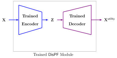
(a)

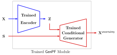
(b)

Figure 8: The $\mathsf{DisPF}$ and $\mathsf{GenPF}$ modules have been trained and are designed for integration in a plug-and-play manner. These modules are characterized by a set of specific parameters: ‘dataset name’ (for example, FairFace), which denotes the dataset utilized; ‘sensitive attribute name’ (e.g., Race); ‘alpha’ (e.g., 0.1); ‘latent $\mathbf{Z}$ dimension’ (e.g., 128); ‘backbone’ (e.g., iResNet 50); ‘loss function’ (e.g., arcface); and ‘backbone trained dataset’ (e.g., WebFace12M).

Table 1: Evaluation of facial recognition models using various backbones and loss functions. Metrics include entropy, mutual information between embeddings and labels (gender and race), and recognition accuracy on the ‘Morph’ and ‘FairFace’ datasets.

				$\mathbf{S}$: Gender						$\mathbf{S}$: Race
				$\mathrm{H}(\mathbf{S})$		$\mathrm{I}(\mathbf{X};\mathbf{S})$		Acc		$\mathrm{H}(\mathbf{S})$		$\mathrm{I}(\mathbf{X};\mathbf{S})$		Acc
Backbone Dataset	Backbone	Loss Function	Applied Dataset	Train	Test	Train	Test	Train	Test	Train	Test	Train	Test	Train	Test
WebFace4M	iResNet18	AdaFace	Morph	0.619	0.621	0.610	0.620	0.999	0.996	0.924	0.933	0.878	0.924	0.998	0.993
WebFace4M	iResNet50	AdaFace	Morph			0.610	0.620	0.999	0.996			0.873	0.930	0.998	0.992
WebFace12M	iResNet101	AdaFace	Morph			0.605	0.622	0.999	0.996			0.873	0.911	0.998	0.992
MS1M-RetinaFace	iResNet50	ArcFace	Morph			0.600	0.620	0.999	0.996			0.865	0.910	0.997	0.993
MS1M-RetinaFace	iResNet100	ArcFace	Morph			0.597	0.618	0.999	0.997			0.868	0.905	0.997	0.993
WebFace4M	iResNet18	AdaFace	FairFace	0.999	0.999	0.930	0.968	0.953	0.923	2.517	2.515	2.099	2.405	0.882	0.763
WebFace4M	iResNet50	AdaFace	FairFace			0.932	0.968	0.954	0.931			2.113	2.409	0.883	0.769
WebFace12M	iResNet101	AdaFace	FairFace			0.934	0.969	0.957	0.930			2.151	2.417	0.892	0.765
MS1M-RetinaFace	iResNet50	ArcFace	FairFace			0.892	0.962	0.950	0.927			1.952	2.355	0.872	0.753
MS1M-RetinaFace	iResNet100	ArcFace	FairFace			0.889	0.954	0.951	0.927			1.949	2.348	0.875	0.765

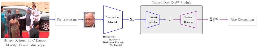
Figure 9: Evaluating the performance of the deep variational $\mathsf{DisPF}$ model, which was trained on the FairFace dataset, when applied to the IJBC test dataset (cross-dataset evaluation). This evaluation highlights the use of $\mathsf{DisPF}$ as a plug-and-play module within the information flow of state-of-the-art face recognition models.

6.6 Experiments Results

6.6.1 Evaluation of Morph and FairFace Datasets Before Applying DVPF

Table 1 depicts the Shannon entropy, estimated mutual information between the extracted embeddings $\mathbf{X}\in\mathbb{R}^{512}$ and sensitive attributes $\mathbf{S}$, and accuracy of classification of $\mathbf{S}$, for test and train sets, before applying our DVPF model. A close proximity between $\mathrm{I}(\mathbf{X};\mathbf{S})$ and entropy $\mathrm{H}(\mathbf{S})$ indicates that the embeddings considerably mitigate label uncertainty. Given $\mathrm{I}(\mathbf{X};\mathbf{S})=\mathrm{H}(\mathbf{X})+\mathrm{H}(\mathbf{S})-\mathrm{H}(\mathbf{X},\mathbf{S})$, mutual information serves as a measure of the reduced joint uncertainty about $\mathbf{X}$ and $\mathbf{S}$. It’s pivotal to note that $\mathrm{I}(\mathbf{X};\mathbf{S})\leq\min\left(\mathrm{H}(\mathbf{X}),\mathrm{H}(\mathbf{S})\right)$. For the Morph/FairFace datasets, the entropy of sensitive attributes (gender or race) remains consistent across both train/test sets and differing FR model embeddings, emphasizing the same dataset usage throughout experiments. Both Morph and FairFace datasets, featuring ‘male’ and ‘female’ gender labels, attain a maximum entropy of $\log_{2}(2)=1$. The Morph dataset, with four distinct race labels, reaches a maximum entropy of $\log_{2}(4)=2$, while the FairFace dataset, with six race labels, tops at $\log_{2}(6)=2.585$. Within Morph, the mutual information for gender mirrors its entropy, suggesting notable preservation of sensitive information in the embeddings. However, for race, values of approximately $0.92\text{-}0.93$ underscore an imbalanced label distribution, as they don’t reach the theoretical $\log_{2}(4)=2$. In contrast, the FairFace dataset displays near-maximal entropies for race ($\sim 2.517$ relative to a potential $2.585$) and gender ($\sim 0.999$ compared to an ideal $1$), illustrating well-balanced racial and gender label distributions.

Table 2: Analysis of the obfuscation-utility trade-off in face recognition models using the iResNet-50 architecture with (P1) and (P2). Performance is evaluated across varying information leakage weights $\alpha$, with significant differences between $\alpha=0.1$ and $\alpha=10$. Sensitive attributes considered are ‘Gender’ and ‘Race’ with a latent dimensionality of $d_{\mathbf{z}}=512$ (top), $d_{\mathbf{z}}=256$ (middle), and $d_{\mathbf{z}}=128$ (down). Notations: “WF4M” represents “WebFace4M”, “MS1M-RF” denotes “MS1M-RetinaFace”, and “TMR” represents “TMR@FMR=10e-1”.

(P1)	$\mathbf{S}$: Gender									$\mathbf{S}$: Race
($d_{\mathbf{z}}=512$)	$\alpha=0.1$			$\alpha=1$			$\alpha=10$			$\alpha=0.1$			$\alpha=1$			$\alpha=10$
Face Recognition Model	TMR	$\mathrm{I}(\mathbf{Z};\mathbf{S})$	Acc on $\mathbf{S}$	TMR	$\mathrm{I}(\mathbf{Z};\mathbf{S})$	Acc on $\mathbf{S}$	TMR	$\mathrm{I}(\mathbf{Z};\mathbf{S})$	Acc on $\mathbf{S}$	TMR	$\mathrm{I}(\mathbf{Z};\mathbf{S})$	Acc on $\mathbf{S}$	TMR	$\mathrm{I}(\mathbf{Z};\mathbf{S})$	Acc on $\mathbf{S}$	TMR	$\mathrm{I}(\mathbf{Z};\mathbf{S})$	Acc on $\mathbf{S}$
WF4M-i50-Ada-Morph	87.31	0.486	0.985	67.55	0.484	0.946	34.42	0.410	0.847	87.13	0.658	0.997	63.51	0.656	0.997	32.58	0.558	0.997
MS1M-RF-i50-Arc-Morph	95.60	0.473	0.991	83.42	0.468	0.970	60.49	0.416	0.846	95.64	0.573	0.997	83.34	0.566	0.997	60.10	0.554	0.997
WF4M-i50-Ada-FairFace	84.00	0.736	0.916	65.66	0.650	0.807	42.97	0.524	0.582	84.30	1.306	0.942	65.51	1.129	0.893	43.18	0.858	0.756
MS1M-RF-i50-Arc-FairFace	93.78	0.680	0.917	83.99	0.677	0.859	61.03	0.586	0.605	93.81	1.090	0.945	84.03	1.005	0.914	61.44	0.830	0.762

(P1)	$\mathbf{S}$: Gender									$\mathbf{S}$: Race
($d_{\mathbf{z}}=256$)	$\alpha=0.1$			$\alpha=1$			$\alpha=10$			$\alpha=0.1$			$\alpha=1$			$\alpha=10$
Face Recognition Model	TMR	$\mathrm{I}(\mathbf{Z};\mathbf{S})$	Acc on $\mathbf{S}$	TMR	$\mathrm{I}(\mathbf{Z};\mathbf{S})$	Acc on $\mathbf{S}$	TMR	$\mathrm{I}(\mathbf{Z};\mathbf{S})$	Acc on $\mathbf{S}$	TMR	$\mathrm{I}(\mathbf{Z};\mathbf{S})$	Acc on $\mathbf{S}$	TMR	$\mathrm{I}(\mathbf{Z};\mathbf{S})$	Acc on $\mathbf{S}$	TMR	$\mathrm{I}(\mathbf{Z};\mathbf{S})$	Acc on $\mathbf{S}$
WF4M-i50-Ada-Morph	91.99	0.464	0.992	46.98	0.444	0.949	29.56	0.388	0.843	91.86	0.628	0.997	47.42	0.705	0.997	30.99	0.550	0.857
MS1M-RF-i50-Arc-Morph	93.30	0.485	0.992	84.08	0.492	0.971	58.62	0.335	0.846	94.01	0.635	0.997	84.10	0.707	0.997	58.24	0.558	0.868
WF4M-i50-Ada-FairFace	92.34	0.638	0.925	63.12	0.653	0.815	39.75	0.367	0.576	92.41	0.866	0.946	58.67	0.950	0.893	38.80	0.595	0.756
MS1M-RF-i50-Arc-FairFace	90.87	0.636	0.915	82.01	0.652	0.860	59.62	0.388	0.598	90.86	0.899	0.947	81.98	0.873	0.919	60.33	0.608	0.766

(P1)	$\mathbf{S}$: Gender									$\mathbf{S}$: Race
($d_{\mathbf{z}}=128$)	$\alpha=0.1$			$\alpha=1$			$\alpha=10$			$\alpha=0.1$			$\alpha=1$			$\alpha=10$
Face Recognition Model	TMR	$\mathrm{I}(\mathbf{Z};\mathbf{S})$	Acc on $\mathbf{S}$	TMR	$\mathrm{I}(\mathbf{Z};\mathbf{S})$	Acc on $\mathbf{S}$	TMR	$\mathrm{I}(\mathbf{Z};\mathbf{S})$	Acc on $\mathbf{S}$	TMR	$\mathrm{I}(\mathbf{Z};\mathbf{S})$	Acc on $\mathbf{S}$	TMR	$\mathrm{I}(\mathbf{Z};\mathbf{S})$	Acc on $\mathbf{S}$	TMR	$\mathrm{I}(\mathbf{Z};\mathbf{S})$	Acc on $\mathbf{S}$
WF4M-i50-Ada-Morph	88.20	0.392	0.988	67.55	0.387	0.952	21.76	0.205	0.845	87.70	0.563	0.998	67.50	0.632	0.997	20.85	0.375	0.997
MS1M-RF-i50-Arc-Morph	97.60	0.358	0.988	85.91	0.320	0.974	62.97	0.278	0.848	97.61	0.574	0.998	86.01	0.603	0.997	62.41	0.421	0.996
WF4M-i50-Ada-FairFace	94.38	0.437	0.892	68.70	0.420	0.809	21.47	0.198	0.546	94.49	0.716	0.937	68.49	0.665	0.892	21.36	0.291	0.733
MS1M-RF-i50-Arc-FairFace	98.03	0.425	0.890	86.07	0.412	0.860	61.11	0.284	0.637	97.77	0.631	0.933	86.07	0.657	0.919	61.25	0.551	0.783

(P2)	$\mathbf{S}$: Gender												$\mathbf{S}$: Race
($d_{\mathbf{z}}=512$)	$\alpha=0.1$			$\alpha=0.5$			$\alpha=1$			$\alpha=10$			$\alpha=0.1$			$\alpha=0.5$			$\alpha=1$			$\alpha=10$
Face Recognition Model	TMR	$\mathrm{I}(\mathbf{Z};\mathbf{S})$	Acc on $\mathbf{S}$	TMR	$\mathrm{I}(\mathbf{Z};\mathbf{S})$	Acc on $\mathbf{S}$	TMR	$\mathrm{I}(\mathbf{Z};\mathbf{S})$	Acc on $\mathbf{S}$	TMR	$\mathrm{I}(\mathbf{Z};\mathbf{S})$	Acc on $\mathbf{S}$	TMR	$\mathrm{I}(\mathbf{Z};\mathbf{S})$	Acc on $\mathbf{S}$	TMR	$\mathrm{I}(\mathbf{Z};\mathbf{S})$	Acc on $\mathbf{S}$	TMR	$\mathrm{I}(\mathbf{Z};\mathbf{S})$	Acc on $\mathbf{S}$	TMR	$\mathrm{I}(\mathbf{Z};\mathbf{S})$	Acc on $\mathbf{S}$
WF4M-i50-Ada-Morph	81.68	0.559	0.986	60.90	0.570	0.966	51.86	0.564	0.945	38.20	0.529	0.853	82.22	0.788	0.998	61.07	0.803	0.997	52.18	0.791	0.997	36.26	0.737	0.996
MS1M-RF-i50-Arc-Morph	91.18	0.552	0.991	77.86	0.572	0.978	73.82	0.562	0.962	67.40	0.524	0.876	91.37	0.765	0.998	77.76	0.796	0.977	73.56	0.794	0.997	67.82	0.751	0.996
WF4M-i50-Ada-FairFace	85.56	0.850	0.918	63.75	0.868	0.885	54.94	0.859	0.853	40.42	0.809	0.759	85.43	1.719	0.944	63.89	1.810	0.926	54.38	1.794	0.908	39.47	1.699	0.839
MS1M-RF-i50-Arc-FairFace	92.20	0.819	0.914	78.34	0.869	0.891	74.08	0.863	0.868	68.00	0.827	0.795	92.15	1.547	0.944	78.26	1.796	0.932	73.36	1.745	0.920	67.65	1.708	0.872

(P2)	$\mathbf{S}$: Gender												$\mathbf{S}$: Race
($d_{\mathbf{z}}=256$)	$\alpha=0.1$			$\alpha=0.5$			$\alpha=1$			$\alpha=10$			$\alpha=0.1$			$\alpha=0.5$			$\alpha=1$			$\alpha=10$
Face Recognition Model	TMR	$\mathrm{I}(\mathbf{Z};\mathbf{S})$	Acc on $\mathbf{S}$	TMR	$\mathrm{I}(\mathbf{Z};\mathbf{S})$	Acc on $\mathbf{S}$	TMR	$\mathrm{I}(\mathbf{Z};\mathbf{S})$	Acc on $\mathbf{S}$	TMR	$\mathrm{I}(\mathbf{Z};\mathbf{S})$	Acc on $\mathbf{S}$	TMR	$\mathrm{I}(\mathbf{Z};\mathbf{S})$	Acc on $\mathbf{S}$	TMR	$\mathrm{I}(\mathbf{Z};\mathbf{S})$	Acc on $\mathbf{S}$	TMR	$\mathrm{I}(\mathbf{Z};\mathbf{S})$	Acc on $\mathbf{S}$	TMR	$\mathrm{I}(\mathbf{Z};\mathbf{S})$	Acc on $\mathbf{S}$
WF4M-i50-Ada-Morph	81.88	0.585	0.987	60.65	0.586	0.971	50.92	0.569	0.953	37.57	0.539	0.873	81.90	0.773	0.998	60.66	0.812	0.997	51.51	0.816	0.997	38.08	0.765	0.996
MS1M-RF-i50-Arc-Morph	91.58	0.539	0.991	77.60	0.575	0.981	72.96	0.580	0.968	67.06	0.549	0.899	91.74	0.792	0.998	77.59	0.812	0.997	73.03	0.812	0.997	67.31	0.776	0.996
WF4M-i50-Ada-FairFace	86.67	0.844	0.916	63.64	0.865	0.892	54.41	0.830	0.865	40.61	0.771	0.762	86.61	1.611	0.944	63.62	1.699	0.930	54.43	1.653	0.916	39.75	1.503	0.855
MS1M-RF-i50-Arc-FairFace	92.34	0.845	0.915	77.51	0.863	0.901	73.00	0.853	0.882	67.51	0.779	0.803	92.35	1.528	0.943	77.48	1.701	0.936	72.76	1.678	0.926	66.90	1.571	0.882

(P2)	$\mathbf{S}$: Gender												$\mathbf{S}$: Race
($d_{\mathbf{z}}=128$)	$\alpha=0.1$			$\alpha=0.5$			$\alpha=1$			$\alpha=10$			$\alpha=0.1$			$\alpha=0.5$			$\alpha=1$			$\alpha=10$
Face Recognition Model	TMR	$\mathrm{I}(\mathbf{Z};\mathbf{S})$	Acc on $\mathbf{S}$	TMR	$\mathrm{I}(\mathbf{Z};\mathbf{S})$	Acc on $\mathbf{S}$	TMR	$\mathrm{I}(\mathbf{Z};\mathbf{S})$	Acc on $\mathbf{S}$	TMR	$\mathrm{I}(\mathbf{Z};\mathbf{S})$	Acc on $\mathbf{S}$	TMR	$\mathrm{I}(\mathbf{Z};\mathbf{S})$	Acc on $\mathbf{S}$	TMR	$\mathrm{I}(\mathbf{Z};\mathbf{S})$	Acc on $\mathbf{S}$	TMR	$\mathrm{I}(\mathbf{Z};\mathbf{S})$	Acc on $\mathbf{S}$	TMR	$\mathrm{I}(\mathbf{Z};\mathbf{S})$	Acc on $\mathbf{S}$
WF4M-i50-Ada-Morph	84.06	0.556	0.984	62.62	0.575	0.973	52.05	0.572	0.963	36.76	0.531	0.906	84.14	0.810	0.998	62.94	0.827	0.997	52.34	0.820	0.997	36.26	0.789	0.996
MS1M-RF-i50-Arc-Morph	93.00	0.541	0.987	79.40	0.573	0.981	73.50	0.572	0.974	66.28	0.535	0.927	93.10	0.800	0.998	79.99	0.828	0.997	74.04	0.825	0.997	65.94	0.793	0.996
WF4M-i50-Ada-FairFace	88.51	0.724	0.893	67.43	0.738	0.870	57.44	0.729	0.854	39.27	0.676	0.800	88.55	1.375	0.938	67.34	1.503	0.926	57.28	1.479	0.916	39.60	1.359	0.877
MS1M-RF-i50-Arc-FairFace	94.14	0.700	0.890	81.81	0.749	0.878	75.95	0.743	0.869	67.16	0.719	0.836	94.23	1.136	0.934	81.67	1.381	0.927	75.96	1.404	0.922	67.16	1.368	0.903

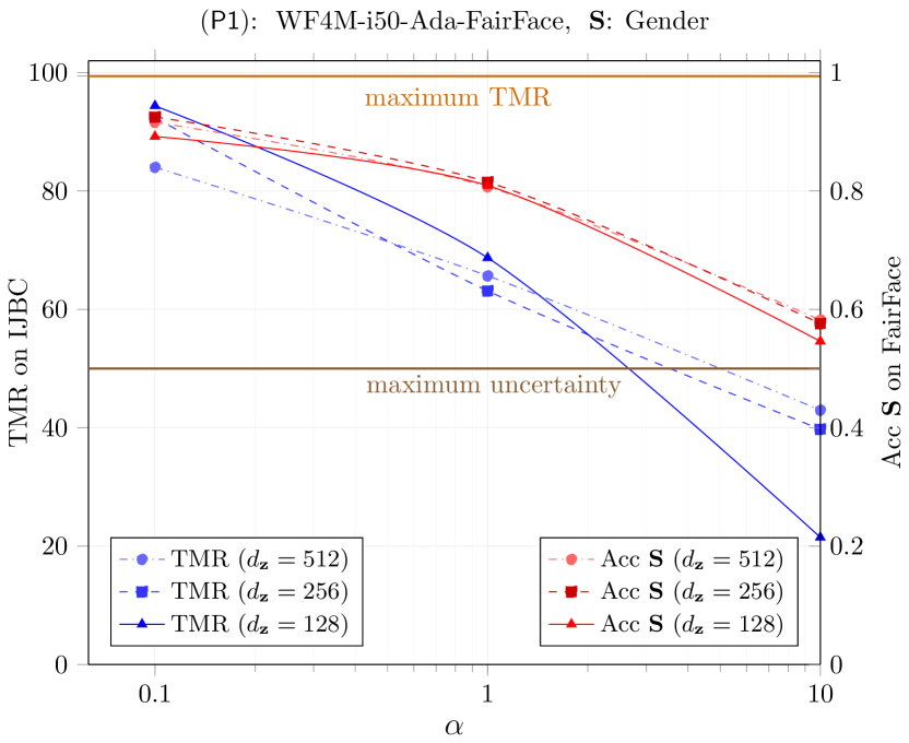
(a)

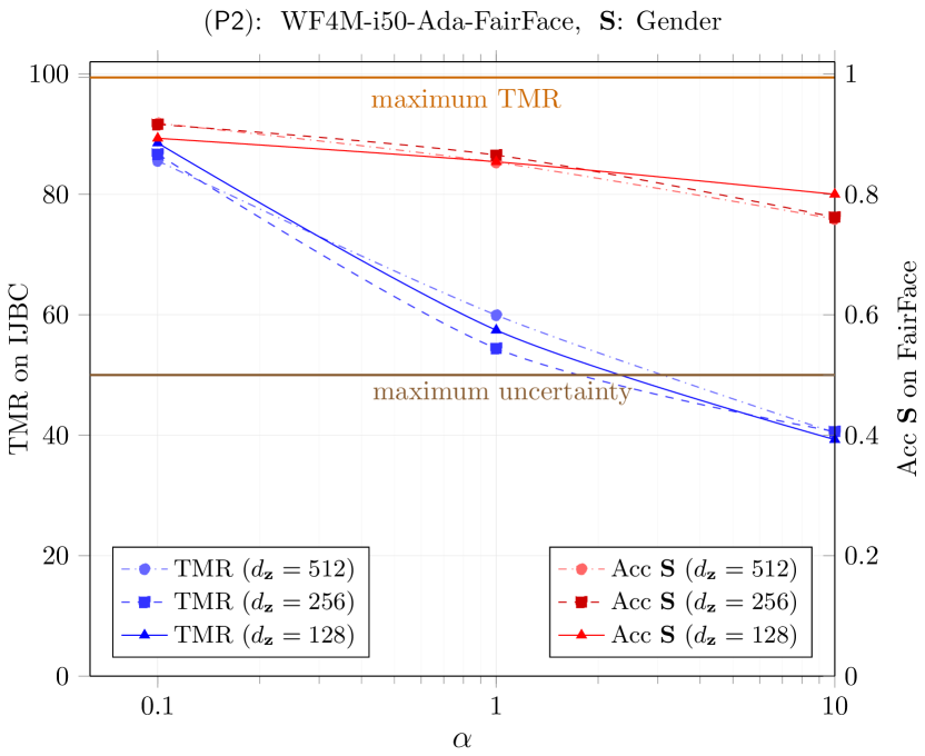
(b)

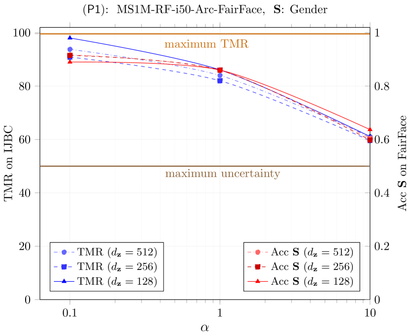
(c)

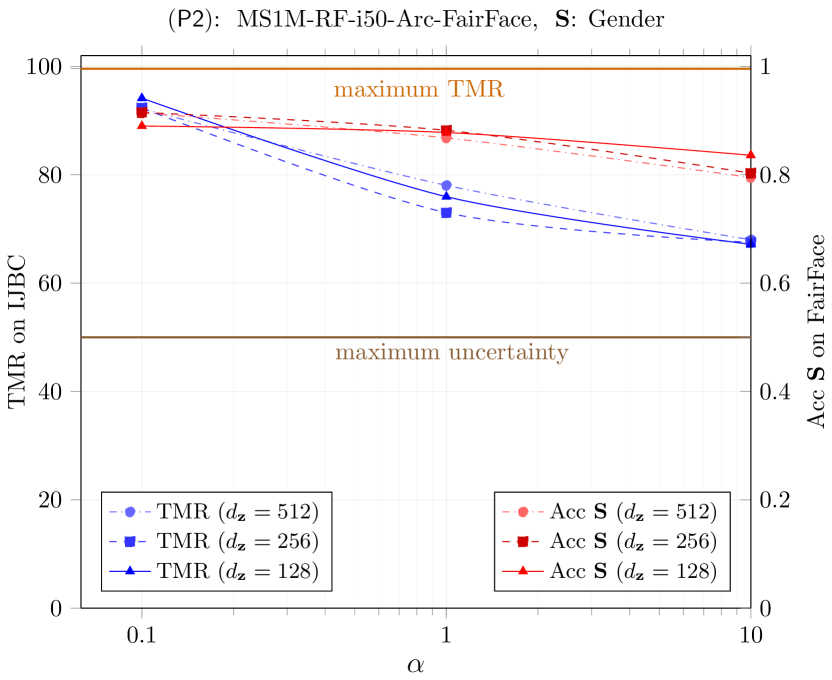
(d)

Figure 10: Trade-off between information utility and privacy leakage using DVPF models for gender attribute: comparing classification accuracy on FairFace and TMR on IJB-C.

6.6.2 Evaluation of Morph and FairFace Datasets After Applying DVPF

We applied our deep variational $\mathsf{DisPF}$ (21) and $\mathsf{GenPF}$ (22) models to the embeddings obtained from the FR models referenced in Table 1. The assessment was initiated with the pre-trained backbones, followed by our $\mathsf{DisPF}$ or $\mathsf{GenPF}$ model, which was developed using embeddings from these pre-trained structures. Figure 7 represents our training framework for the deep $\mathsf{DisPF}$ problem, using iResNet50 as the backbone, WebFace4M as the backbone dataset, and ArcFace for the FR loss. The applied dataset is FairFace, with race as the sensitive attribute. We considered a similar embedding-based learning framework for the deep $\mathsf{GenPF}$ problem. Given the consistent accuracy for sensitive attribute $\mathbf{S}$ and similar information leakage $\mathrm{I}\left(\mathbf{X};\mathbf{S}\right)$ observed across various iResNet architectures, we present results specific to iResNet50. Figure 8 depicts the trained modules that we will use during the inference phase for both same-dataset evaluations (where the models are tested on unseen portions of the dataset they were trained on) and cross-dataset evaluations (where the models are tested on entirely different datasets to assess their ability to generalize to new data)

In Table 2, we precisely quantify the disclosed information leakage, represented as $\mathrm{I}(\mathbf{S};\mathbf{Z})$. Additionally, we provide a detailed account of the accuracy achieved in recognizing sensitive attributes from the disclosed representation $\mathbf{Z}\in\mathbb{R}^{256}$, utilizing a support vector classifier optimization. These evaluations are based on test sets derived from either the Morph or FairFace datasets. Consistent with our expectations, as $\alpha$ increases towards infinity ($\alpha\rightarrow\infty$), the information leakage $\mathrm{I}(\mathbf{S};\mathbf{Z})$ decreases to zero. At the same time, the recognition accuracy for the sensitive attribute $\mathbf{S}$ approaches $0.5$, indicative of random guessing.

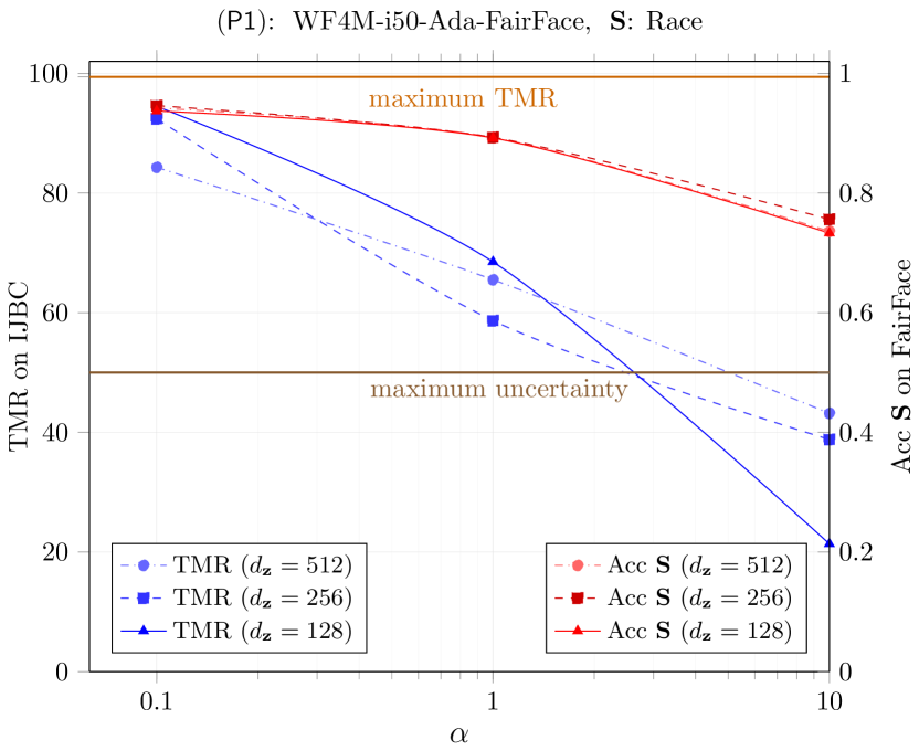
(a)

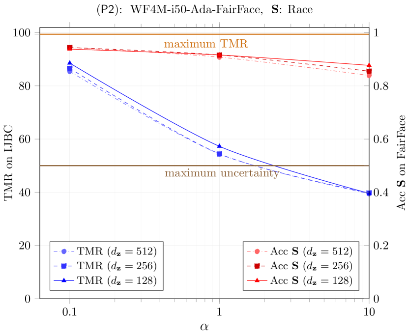
(b)

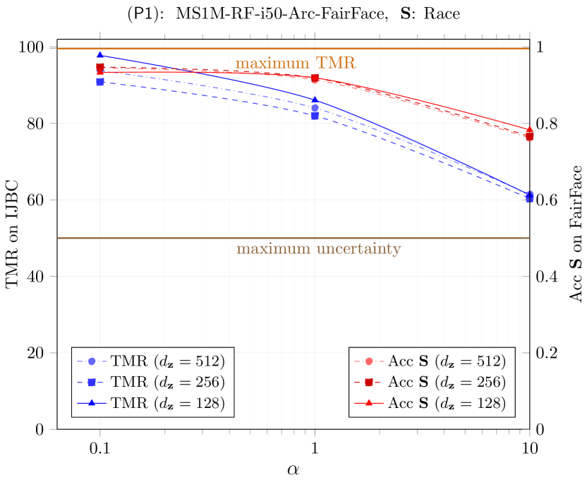
(c)

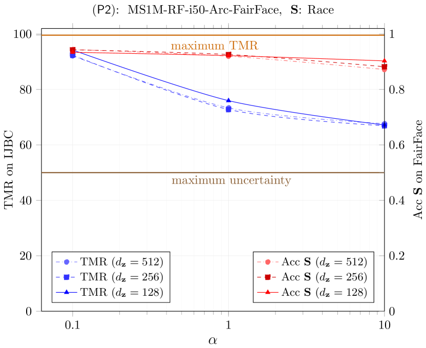
(d)

Figure 11: Trade-off between information utility and privacy leakage using DVPF models for race attribute: comparing classification accuracy on FairFace and TMR on IJB-C.

6.6.3 TMR Benchmark on IJB-C in FairFace Experiments

To evaluate the generalization of our mechanisms in terms of FR accuracy, we utilized the challenging IJB-C test dataset (Maze et al., 2018) as a challenging benchmark. Figure 9 depicts our inference framework, which incorporates the $\mathsf{DisPF}$ trained module. We employ a similar inference framework for the $\mathsf{GenPF}$ trained module. We detail the $\mathsf{TMR}$ of our models in Table 2. It’s imperative to note that all these evaluations are systematically benchmarked against a predetermined False Match Rate ($\mathsf{FMR}$) of $10^{-1}$.When subjecting the ‘WF4M-i50-Ada’ model to evaluation against the IJB-C dataset—prior to the DVPF model’s integration—a $\mathsf{TMR}$ of $\mathsf{99.40\%}$ at $\mathsf{FMR=10e-1}$ was observed. Similarly, for the ‘MS1M-RF-i50-Arc’ configuration, a $\mathsf{TMR}$ of $\mathsf{99.58\%}$ was observed on the IJB-C dataset before the integration of the DVPF model, with measurements anchored to the same $\mathsf{FMR}$. In Figure 10 and Figure 11, we demonstrate the interplay between information utility and privacy leakage across varying information leakage weights $\alpha$. The right y-axis quantifies the classification accuracy of the sensitive attribute $\mathbf{S}$, as evaluated on the FairFace dataset. In contrast, the left y-axis depicts the $\mathsf{TMR}$ on the IJB-C test dataset. This measurement is derived from the performance of trained Deep Variational Privacy Filtering (DVPF) models $(\textsf{P1})$ and $(\textsf{P2})$, initially trained on the FairFace dataset and subsequently tested on the IJB-C dataset.

Figure 10 focuses on the results obtained using the WF4M-i50-Ada-FairFace configuration (where ‘Backbone Dataset’ is WebFace4M, ‘Backbone Architecture’ is iResNet50, ‘Loss Function’ is AdaFace, and ‘Applied Dataset’ for training is FairFace, ‘Dataset for Testing Utility’ ($\mathsf{TMR}$) being IJB-C) and MS1M-RF-i50-Arc-FairFace configuration (with ‘Backbone Dataset’ as MS1M-RetinaFace, ‘Backbone Architecture’ as iResNet50, ‘Loss Function’ as ArcFace, and ‘Applied Dataset’ for training as FairFace; ‘Dataset for Testing Utility’ ($\mathsf{TMR}$) being IJB-C) when the sensitive attribute under consideration for training is gender. Figure 11 presents analogous results, but for cases where the sensitive attribute for training is race.

6.6.4 Visualizing DVPF Effects on FairFace and IJB-C Data with t-SNE

Figure 12 and Figure 13 provide qualitative visualization of the leakage in sensitive attribute classification on the FairFace database, both before and after applying the DVPF model with $\mathbf{S}$ set as race or gender, respectively. For this, we use t-distributed stochastic neighbor embedding (t-SNE) (Maaten and Hinton, 2008) to project the underlying space into 2D. As illustrated, distinct regions associated with six racial classes (Asian, Black, Hispanic, Indian, Middle-Eastern, White) are evident in the clean embedding. However, after applying the DVPF (P1) mechanism with $\alpha=10$, the sensitive labels become almost uniformly distributed across the space. This distribution aligns with our interpretation of random guessing performance on the adversary’s side. This behavior is consistent for both ArcFace and AdaFace protected embeddings, and for both gender and race as sensitive attributes. However, for brevity, we present only one example. Figure 14 depicts the normalized confusion matrices for the FairFace dataset, obtained after applying the DVPF (P1) mechanism. In these matrices, $\mathbf{S}$ is considered as race, and the configuration is MS1M-RF-i50-Arc-FairFace, with $\alpha$ values set at $0.1$ and $10$. Notably, as $\alpha$ increases, the diagonal dominance in the matrices becomes less pronounced, indicating a higher probability of misclassification of the sensitive attribute.

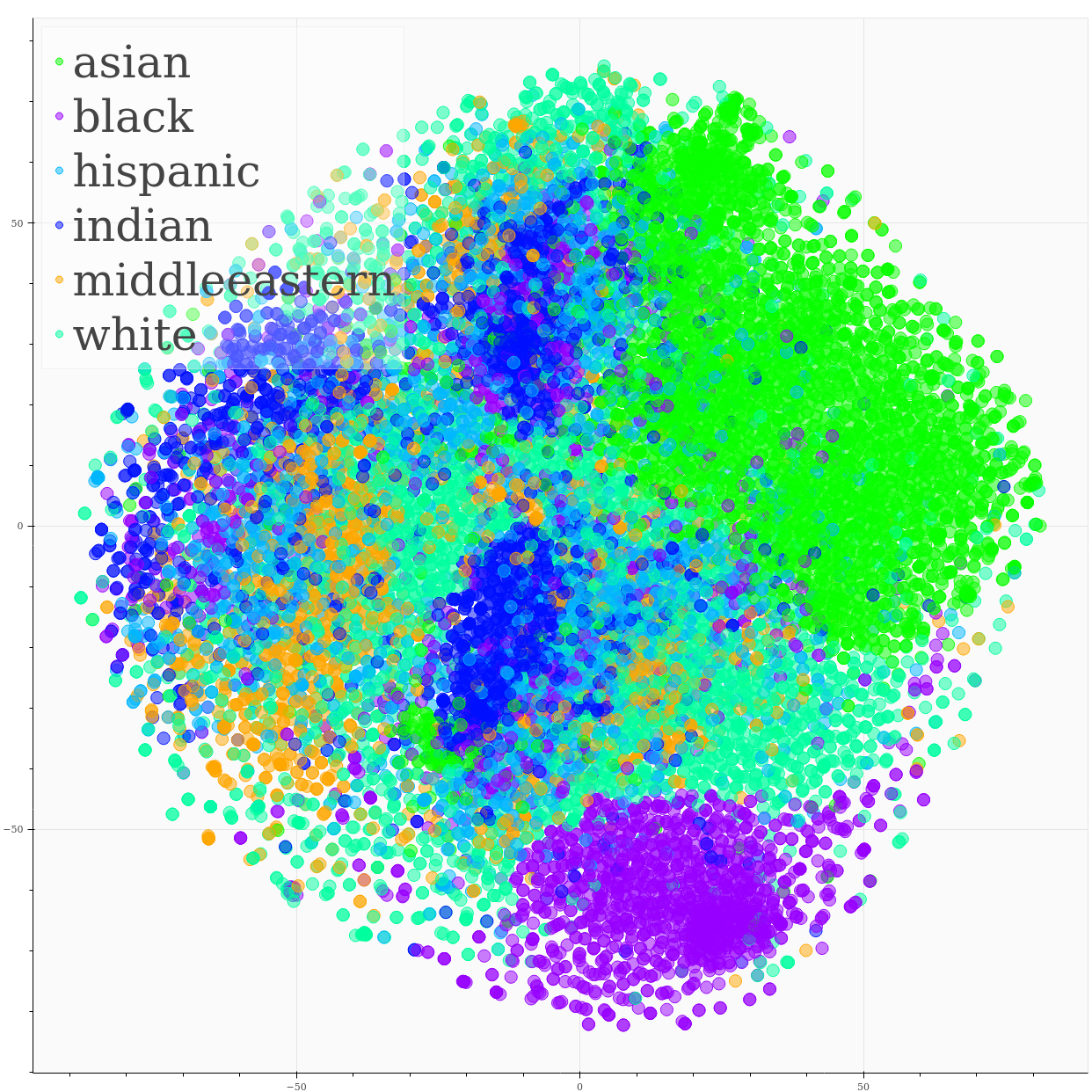
(a)

(b)

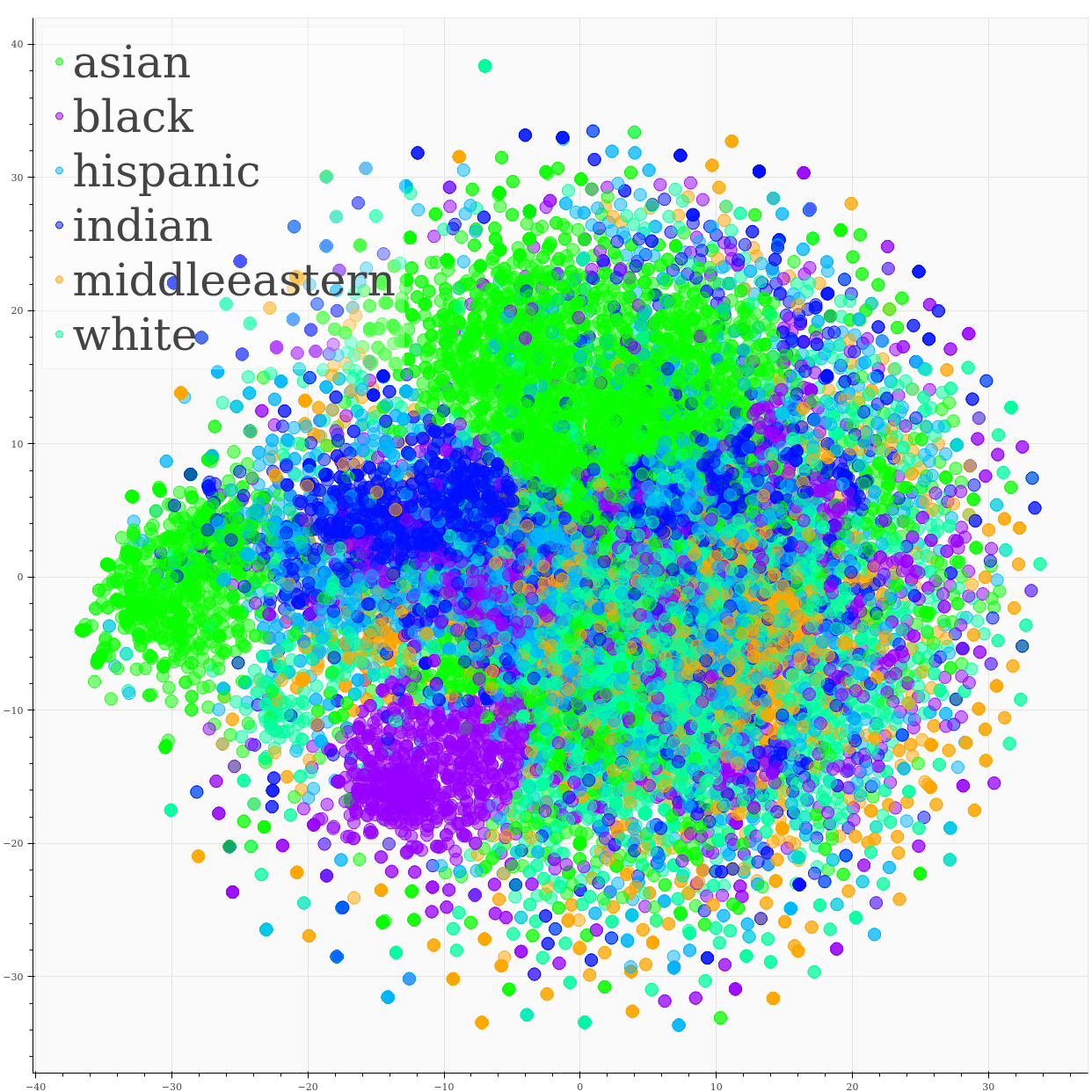
(c)

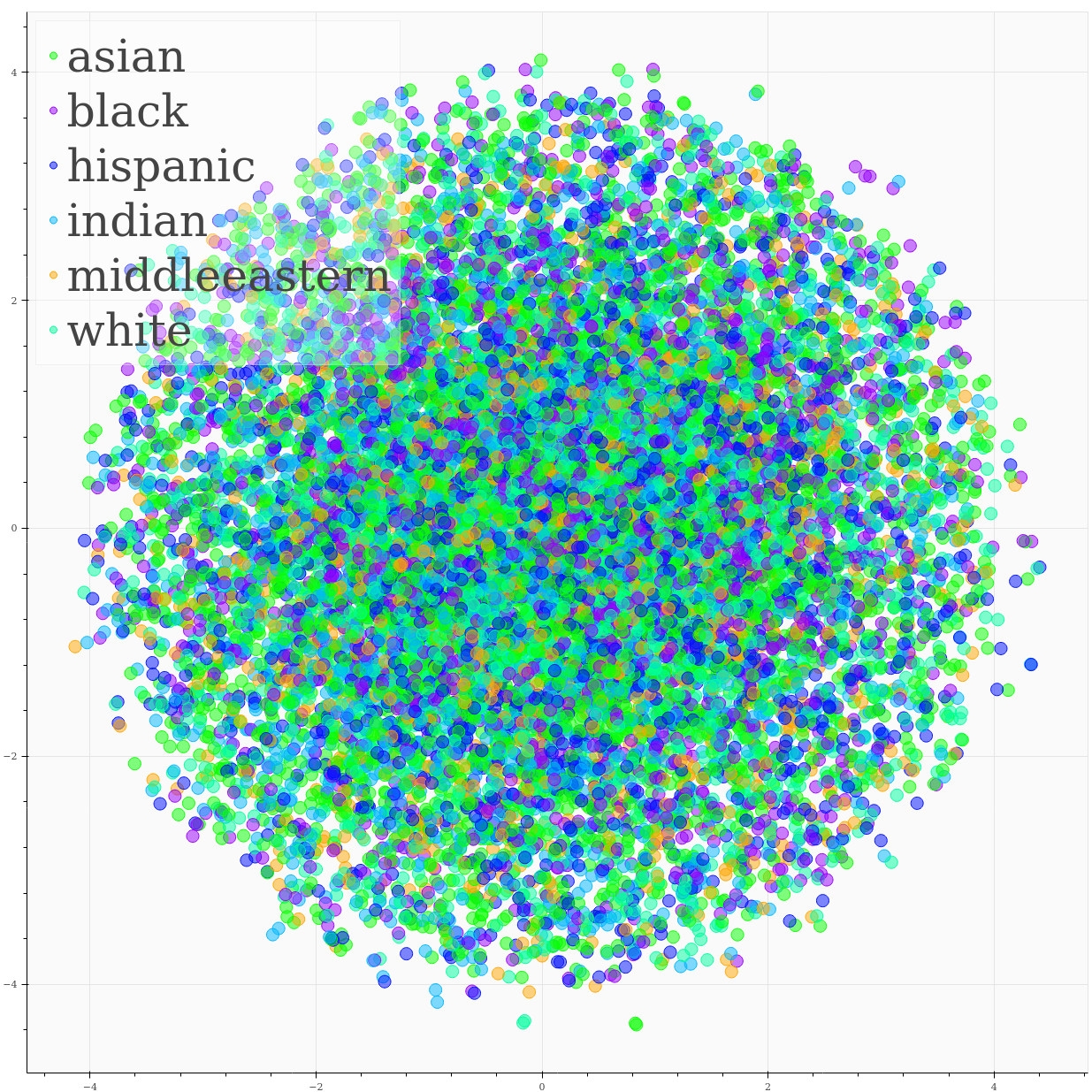
(d)

Figure 12: t-SNE visualizations of the FairFace dataset with $\mathbf{S}$ representing ‘race’, using the (P2) model, setting $\alpha=10$ and $d_{\mathbf{z}}=128$. The visualizations include: (a) AdaFace original (clean) embeddings, (b) Post-DVPF AdaFace embeddings, (c) ArcFace original (clean) embeddings, and (d) Post-DVPF ArcFace embeddings.

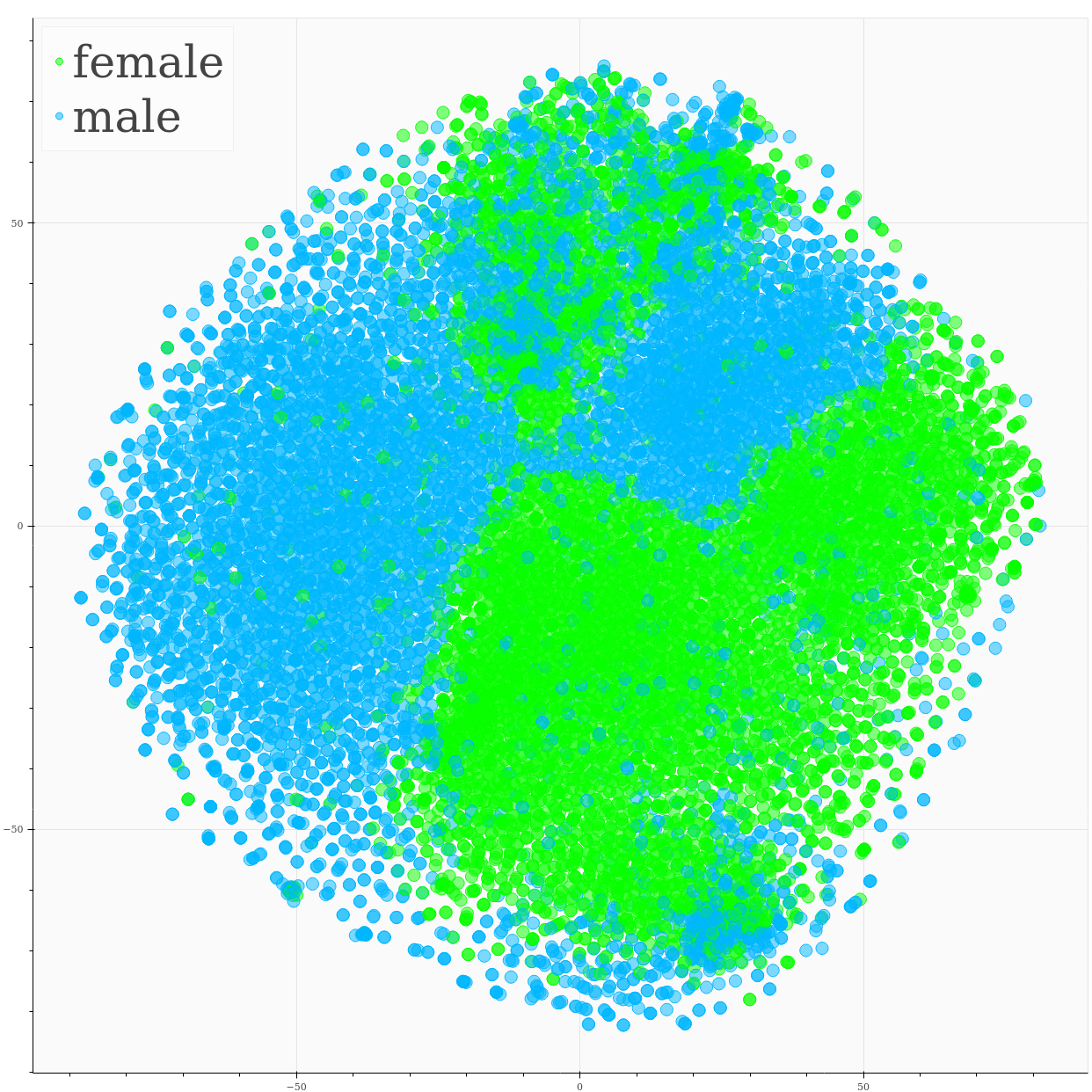
(a)

(b)

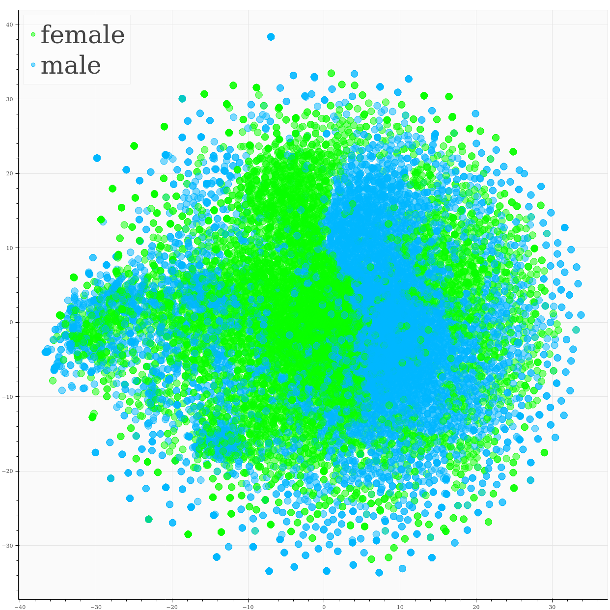
(c)

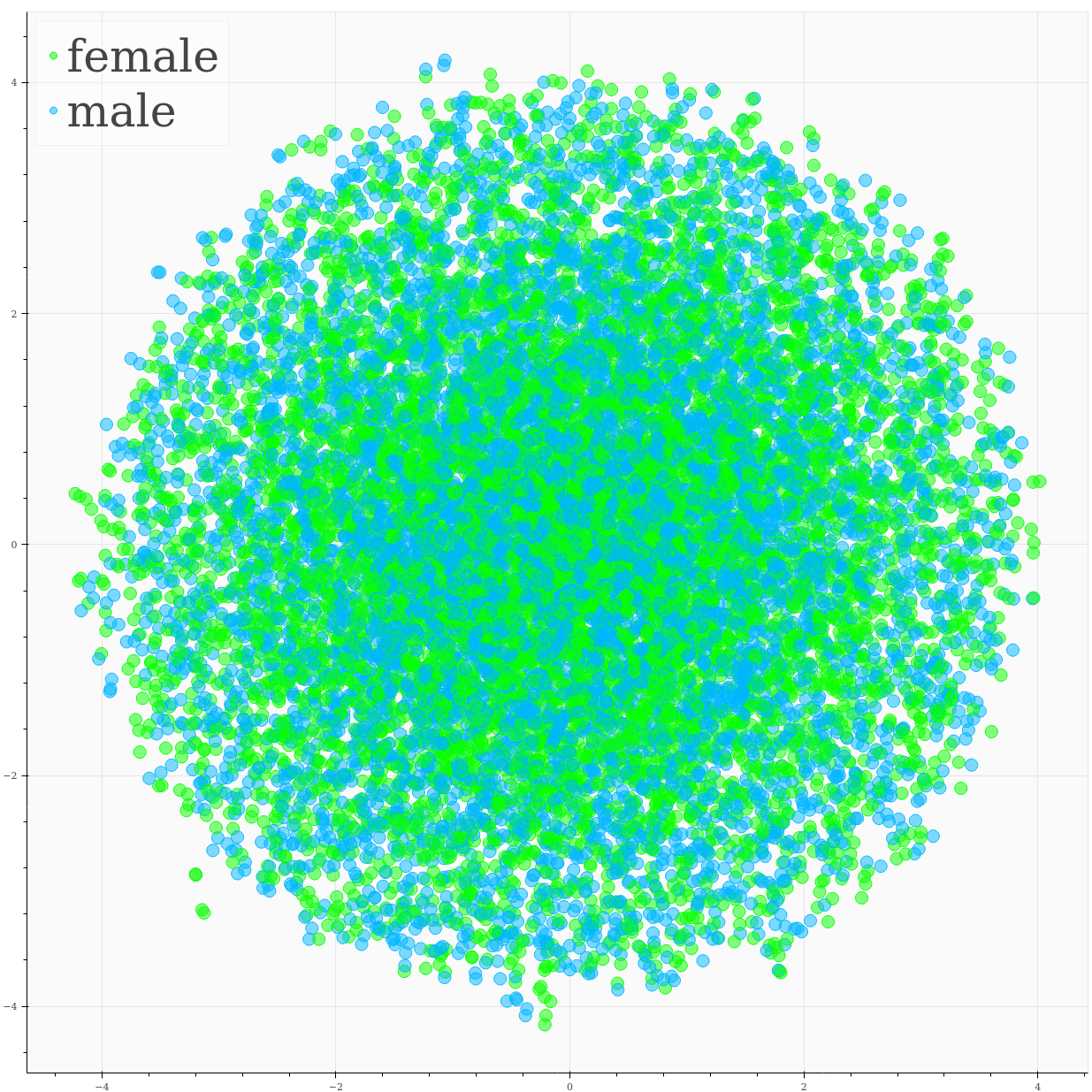
(d)

Figure 13: t-SNE visualizations of the FairFace dataset with $\mathbf{S}$ representing ‘gender’, using the (P2) model, setting $\alpha=10$ and $d_{\mathbf{z}}=128$. The visualizations include: (a) AdaFace original (clean) embeddings, (b) Post-DVPF AdaFace embeddings, (c) ArcFace original (clean) embeddings, and (d) Post-DVPF ArcFace embeddings.

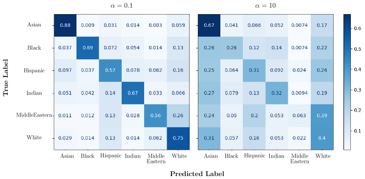
Figure 14: Normalized confusion matrices for the FairFace dataset, considering $\mathbf{S}$ as race, with $\alpha$ values of $0.1$ and $10$.

Figure 15 presents t-SNE visualizations of 10 randomly selected identities from the IJB-C dataset: (a) and (c) show the original (clean) embeddings from ArcFace and AdaFace, respectively, while (b) and (d) depict the obfuscated embeddings of the corresponding FR models using the DVPF (P1) mechanism with $\alpha=0.1$. Notably, increasing the information leakage weight $\alpha$ results in more overlapping regions among identities in this illustrative 2D visualization method.

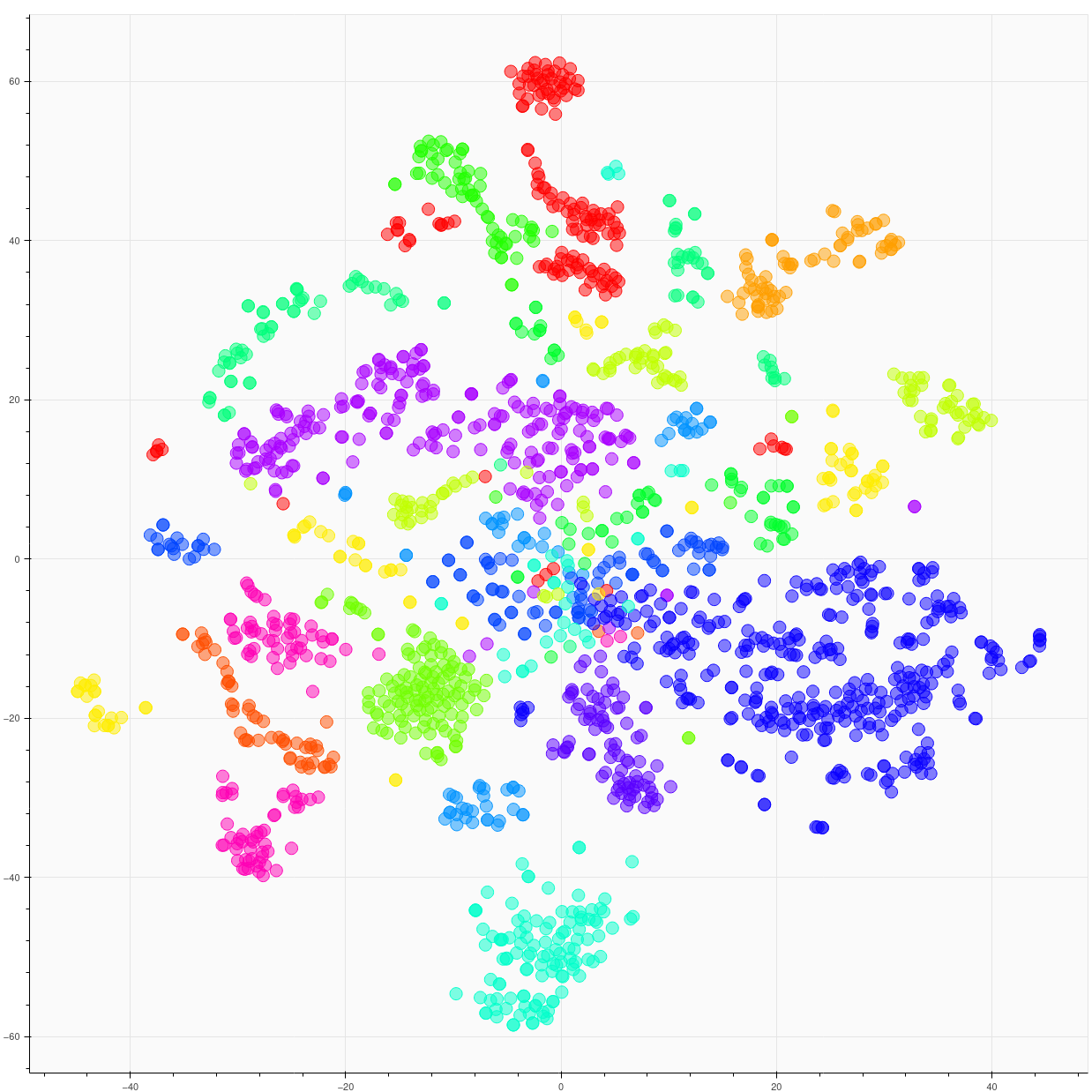
(a)

(b)

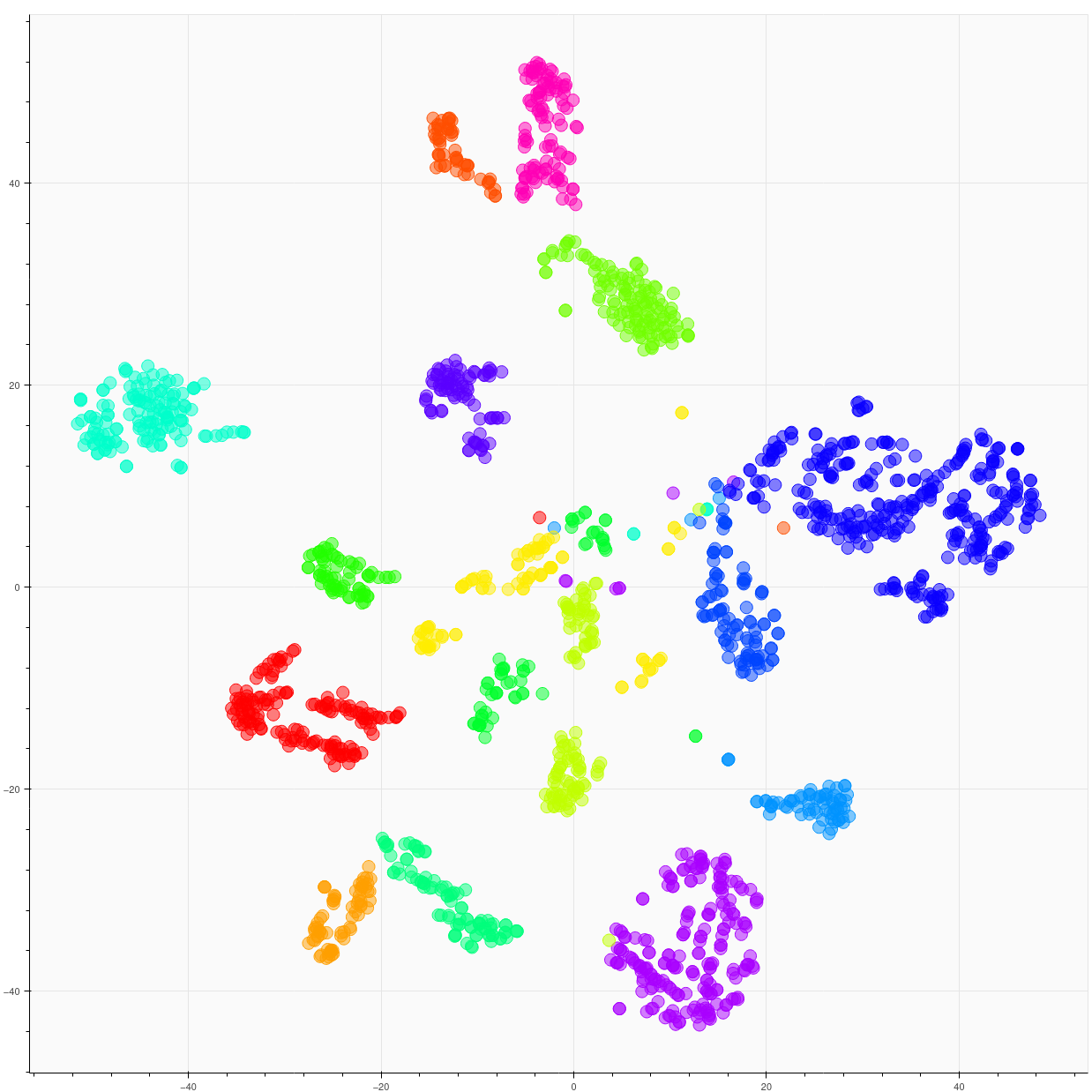
(c)

(d)

Figure 15: t-SNE visualizations of 16 randomly selected identities on the IJB-C dataset: (a) ArcFace, (b) ArcFace with DVPF, (c) AdaFace, (d) AdaFace with DVPF.

6.7 Discussions and Future Directions

6.7.1 Contribution of $\mathsf{GenPF}$ for Bias Mitigation

The proposed $\mathsf{GenPF}$ model can also contribute to mitigating bias through two distinct mechanisms:

Generation of Unbiased Synthetic Datasets for Utility Services Training and Evaluation:

Assuming the conditional generator $g_{\bm{\varphi}}$ possesses the capability to generate high-fidelity synthetic data conditioned on a random variable $\mathbf{S}$ supported on set $\mathcal{S}$, the system designer is thus enabled to produce a synthetic dataset encompassing all potential states of $\mathbf{S}$. The primary objective in this context is to calibrate the entropy $\mathrm{H}\left(P_{\mathbf{\widetilde{S}}}\right)$ to be equal to $\log_{2}|\mathcal{S}|$. Here, $|\mathcal{S}|$ denotes the cardinality, i.e., the total number of unique elements contained within $\mathcal{S}$.

Learning Invariant Representations with Respect to Variable $\mathbf{S}$:

Noting that the $\mathsf{GenPF}$ objective (22) forces the latent representation $\mathbf{S}$ to be independent of the sensitive attribute $\mathbf{S}$ by minimizing $\mathrm{H}_{\bm{\phi},\bm{\varphi}}^{\mathrm{U}}\left(\mathbf{X}\mid\mathbf{S},\mathbf{Z}\right)$, it promotes the representation $\mathbf{Z}$ that is invariant to the variable $\mathbf{S}$. This is one of the primary goals of the in-processing bias mitigation techniques in machine learning which is to reduce undesired bias during the model’s training phase. This approach parallels classical tasks in computer vision, such as identifying features invariant to covariate factors like image translation, scaling, and rotation (Lowe, 1999). An analogous concept is seen in the ‘Fader Network’ (Lample et al., 2017), where the encoder is adversarially trained to ascertain deterministic feature representations, invariant to facial attributes.

6.7.2 Limitations

Optimal Network Architecture:

The pursuit of an optimal network architecture, particularly for the encoder, utility decoder, and uncertainty decoder, remains a central challenge. This complexity arises from the need to balance the encoder’s capability to capture nuanced features with the utility decoder’s and the (conditional) uncertainty decoder’s abilities to reconstruct utility data and generate conditioned data. Determining the most effective architecture necessitates a nuanced understanding of the interplay between these components, which is highly dependent on the specific dataset and application domain under consideration.

Fine-tuning Limitations:

The model’s complexity, compounded by the extensive array of hyper-parameters, introduces significant fine-tuning limitations. These constraints not only hinder the optimization process but also limit the model’s adaptability to new datasets. The relationship between hyper-parameter configurations and model performance emphasizes the necessity for advanced methods in hyper-parameter optimization to navigate this complex landscape effectively.

Alternative Learning Algorithms:

The exploration of alternative learning algorithms represents a promising direction to address the current model’s architectural and fine-tuning challenges. Such algorithms could provide more sophisticated mechanisms for managing the model’s complexity, enhancing its adaptability, and improving scalability across various datasets.

Challenges with Fixed Pretrained Backbones:

Employing fixed pretrained backbones, such as those from face recognition models, without the ability to fine-tune, poses specific challenges. This limitation can significantly impact the model’s flexibility and performance, underscoring the need for strategies that can adapt to or compensate for the constraints of using fixed pre-trained models.

6.7.3 Future Directions

Integration with Prior-Independent Privacy Mechanisms:

Regarding future directions, integrating prior-independent privacy mechanisms, such as differential privacy, with our deep privacy funnel model—whether discriminative or generative—offers a promising research avenue. This integration, effectively combining prior-dependent and prior-independent mechanisms, could significantly enhance our model’s privacy protections. We can ensure comprehensive privacy assurances across various scenarios by addressing both ‘context-free’ and ‘context-aware’ privacy definitions.

Expanding Model Capabilities:

Future research should also explore extending various sections of our general model formulation by employing alternative methods in both the generative and discriminative components. In terms of generative modeling, recent diffusion models have demonstrated significant generative capabilities compared to other generative modeling approaches, such as GANs and VAEs, especially regarding the stability of training and the fidelity of generated data. Similarly, for the discriminative component, the exploration of other architectures, like Vision Transformers (ViTs), should be considered. These architectures offer superior representation of the relationships between different parts of images due to their inherent inductive bias. Such adaptability would enable a broader range of applications, catering to diverse data types and addressing privacy concerns more effectively.

7 Conclusion

This study marks the first integration of privacy funnel analysis into face recognition systems, bridging the gap between information-theoretic privacy and practical deep learning applications. We introduced the generative privacy funnel ($\mathsf{GenPF}$) alongside the discriminative privacy funnel ($\mathsf{DisPF}$), offering new insights into synthetic data generation with privacy guarantees. Our deep variational privacy funnel (DVPF) model, applied to state-of-the-art face recognition systems, demonstrates a quantifiable balance between information obfuscation and utility. Experimental results using advanced FR architectures and datasets highlight the effectiveness of our approach, especially in reducing information leakage about sensitive attributes. Crucially, we evaluated the trained DVPF networks on the challenging IJB-C test dataset. This work provides a robust framework and versatile tools for future privacy-preserving research in facial recognition technologies, with an accompanying reproducible software package facilitating further research exploration and adoption.

A Connecting the Privacy Funnel Method with Other Models

A.1 Connection with Information Bottleneck Model

In contrast to the Privacy Funnel (PF) model, which aims to obtain a representation $\mathbf{Z}$ that minimizes information leakage about $\mathbf{S}$ while maximizing information utility about $\mathbf{X}$, the Information Bottleneck (IB) model (Tishby et al., 2000) focuses on extracting relevant information from the random variable $\mathbf{X}$ about an associated random variable $\mathbf{U}$ of interest. Given two correlated random variables $\mathbf{U}$ and $\mathbf{X}$ with a joint distribution $P_{\mathbf{U,X}}$, the objective of the original IB model is to find a representation $\mathbf{Z}$ of $\mathbf{X}$ through a stochastic mapping $P_{\mathbf{Z}\mid\mathbf{X}}$ that satisfies: (i) $\mathbf{U}\hbox{$\--$}\kern-1.5pt\hbox{$\circ$}\kern-1.5pt\hbox{$\--$}\mathbf{X}\hbox{$\--$}\kern-1.5pt\hbox{$\circ$}\kern-1.5pt\hbox{$\--$}\mathbf{Z}$, and (ii) representation $\mathbf{Z}$ is maximally informative about $\mathbf{U}$ (maximizing $\mathrm{I}\left(\mathbf{U};\mathbf{Z}\right)$) while being minimally informative about $\mathbf{X}$ (minimizing $\mathrm{I}\left(\mathbf{X};\mathbf{Z}\right)$). This trade-off can be expressed by the bottleneck functional:

$$\mathsf{IB}\left(R^{\mathrm{u}},P_{\mathbf{U},\mathbf{X}}\right)\coloneqq\mathop{\inf}_{\begin{subarray}{c}P_{\mathbf{Z}\mid\mathbf{X}}:\\ \mathbf{U}\hbox{$\--$}\kern-1.5pt\hbox{$\circ$}\kern-1.5pt\hbox{$\--$}\mathbf{X}\hbox{$\--$}\kern-1.5pt\hbox{$\circ$}\kern-1.5pt\hbox{$\--$}\mathbf{Z}\end{subarray}}\mathrm{I}\left(\mathbf{X};\mathbf{Z}\right)\;\;\mathrm{s.t.}\;\;\mathrm{I}\left(\mathbf{U};\mathbf{Z}\right)\geq R^{\mathrm{u}}.$$ (39)

In the IB model, $\mathrm{I}\left(\mathbf{U};\mathbf{Z}\right)$ is referred to as the relevance of $\mathbf{Z}$, and $\mathrm{I}\left(\mathbf{X};\mathbf{Z}\right)$ is called the complexity of $\mathbf{Z}$. Since mutual information is defined as Shannon information, the complexity here is quantified by the minimum description length of compressed representation $\mathbf{Z}$. The IB curve is defined by the values $\mathsf{IB}\left(R,P_{\mathbf{U},\mathbf{X}}\right)$ for different $R$. Similarly, by introducing a Lagrange multiplier $\beta\geq 0$, the IB problem can be represented by the associated Lagrangian functional:

$$\mathcal{L}_{\mathrm{IB}}\left(P_{\mathbf{Z}\mid\mathbf{X}},\beta\right)\coloneqq\mathrm{I}\left(\mathbf{X};\mathbf{Z}\right)-\beta\,\mathrm{I}\left(\mathbf{U};\mathbf{Z}\right).$$ (40)

The formulation of the IB method in (Tishby et al., 2000) has inspired numerous characterizations, generalizations, and applications (Makhdoumi et al., 2014; Tishby and Zaslavsky, 2015; Alemi et al., 2016; Strouse and Schwab, 2017; Vera et al., 2018; Kolchinsky et al., 2019; Bang et al., 2019; Amjad and Geiger, 2019; Hu et al., 2019; Wu et al., 2019; Fischer, 2020; Federici et al., 2020; Ding and Sadeghi, 2019; Hafez-Kolahi and Kasaei, 2019; Hafez-Kolahi et al., 2020; Kirsch et al., 2020). For a review of recent research on IB models, we refer the reader to (Voloshynovskiy et al., 2019; Goldfeld and Polyanskiy, 2020; Zaidi et al., 2020; Asoodeh and Calmon, 2020; Razeghi et al., 2023).

A.2 Connection with Complexity-Leakage-Utility Bottleneck Model

Given three dependent (correlated) random variables $\mathbf{U}$, $\mathbf{S}$ and $\mathbf{X}$ with joint distribution $P_{\mathbf{U,S,X}}\,$, the goal of the CLUB model (Razeghi et al., 2023) is to find a representation $\mathbf{Z}$ of $\mathbf{X}$ using a stochastic mapping $P_{\mathbf{Z}\mid\mathbf{X}}$ such that: (i) $\left(\mathbf{U},\mathbf{S}\right)\hbox{$\--$}\kern-1.5pt\hbox{$\circ$}\kern-1.5pt\hbox{$\--$}\mathbf{X}\hbox{$\--$}\kern-1.5pt\hbox{$\circ$}\kern-1.5pt\hbox{$\--$}\mathbf{Z}$, and (ii) representation $\mathbf{Z}$ is maximally informative about $\mathbf{U}$ (maximizing $\mathrm{I}\left(\mathbf{U};\mathbf{Z}\right)$) (iii) while being minimally informative about $\mathbf{X}$ (minimizing $\mathrm{I}\left(\mathbf{X};\mathbf{Z}\right)$) and (iv) minimally informative about $\mathbf{S}$ (minimizing $\mathrm{I}\left(\mathbf{S};\mathbf{Z}\right)$). We can formulate this three-dimensional trade-off by imposing constraints on the two of them. That is, for a given information complexity and information leakage constraints, $R^{\mathrm{z}}\geq 0$ and $R^{\mathrm{s}}\geq 0$, respectively, this trade-off can be formulated by a CLUB functional:

$$\mathsf{CLUB}\left(R^{\mathrm{z}},R^{\mathrm{s}},P_{\mathbf{U},\mathbf{S},\mathbf{X}}\right)\coloneqq\mathop{\sup}_{\begin{subarray}{c}P_{\mathbf{Z}\mid\mathbf{X}}:\\ \left(\mathbf{U},\mathbf{S}\right)\hbox{$\--$}\kern-1.5pt\hbox{$\circ$}\kern-1.5pt\hbox{$\--$}\mathbf{X}\hbox{$\--$}\kern-1.5pt\hbox{$\circ$}\kern-1.5pt\hbox{$\--$}\mathbf{Z}\end{subarray}}\mathrm{I}\left(\mathbf{U};\mathbf{Z}\right)\;\quad\;\mathrm{s.t.}\quad\mathrm{I}\left(\mathbf{X};\mathbf{Z}\right)\leq R^{\mathrm{z}},\;\;\mathrm{I}\left(\mathbf{S};\mathbf{Z}\right)\leq R^{\mathrm{s}}.$$ (41)

Setting $\mathbf{U}\equiv\mathbf{X}$ and $R^{\mathrm{z}}\geq\mathrm{H}\left(P_{\mathbf{X}}\right)$ in the CLUB objective (41), the CLUB model reduces to the discriminative (classical) PF model (7).

A.3 Connection with Image-to-Image Transition Models

Consider two measurable spaces $\mathcal{X}$ and $\mathcal{Y}$. Let $\mathbf{X}\sim P_{\mathbf{X}}$ and $\mathbf{Y}\sim P_{\mathbf{Y}}$ be random objects representing random realizations from these spaces, with distributions $P_{\mathbf{X}}$ and $P_{\mathbf{Y}}$ respectively, where $\mathbf{X}\in\mathcal{X}$ and $\mathbf{Y}\in\mathcal{Y}$. Let $f:\mathcal{X}\rightarrow\mathcal{Y}$ and $g:\mathcal{Y}\rightarrow\mathcal{X}$ denote appropriate mappings (or functions) that map elements between these spaces.

The objective of the image-to-image translation problem is to find (learn) a mapping $f:\mathcal{X}\rightarrow\mathcal{Y}$ (or vice versa $g:\mathcal{Y}\rightarrow\mathcal{X}$) such that (i) the distribution of the mapped object approximates the distribution of the target object, i.e., $P_{f\left(\mathbf{X}\right)}\approx P_{\mathbf{Y}}$ and/or $P_{\mathbf{X}}\approx P_{g\left(\mathbf{Y}\right)}$; and (ii) the mapping preserves or captures specific characteristics or features of the input images. This can be formally expressed as a constraint optimization problem, where the mapped images maintain certain predefined properties or metrics of similarity with the input images. This is a fundamental aspect of tasks like style transfer, domain adaptation, or generative modeling.

Let $\mathcal{C}_{\mathsf{U}}\big{(}P_{f\left(\mathbf{X}\right),\mathbf{Y}}\big{)}=\mathsf{dist}\left(P_{f\left(\mathbf{X}\right)},P_{\mathbf{Y}}\right)$, where $\mathsf{dist}\left(P_{f\left(\mathbf{X}\right)},P_{\mathbf{Y}}\right)$ is a discrepancy measure between $P_{f\left(\mathbf{X}\right)}$ and $P_{\mathbf{Y}}$. For instance, one can consider $\mathsf{dist}(P_{f\left(\mathbf{X}\right)},P_{\mathbf{Y}})=\mathrm{D}_{\mathsf{f}}(P_{f\left(\mathbf{X}\right)}\|P_{\mathbf{Y}})$, or alternatively, one can use the Maximum Mean Discrepancy (MMD) for a characteristic positive-definite reproducing kernel (Tolstikhin et al., 2018). Now, we can consider an optimization problem where the objective is to minimize a loss function that quantifies both the distributional similarity and the preservation of image characteristics:

$$\mathop{\min}_{f,g}\;\;\;\mathsf{dist}\left(P_{f\left(\mathbf{X}\right)},P_{\mathbf{Y}}\right)+\mathsf{dist}(P_{g\left(\mathbf{Y}\right)},P_{\mathbf{X}})+\lambda_{x}\Phi_{x}(\mathbf{X},f\left(\mathbf{X}\right))+\lambda_{y}\Phi_{y}(\mathbf{Y},g\left(\mathbf{Y}\right)).$$ (42)

We can leverage image-to-image transition models from this perspective within a domain-preserving privacy funnel method. This method diverges from traditional obfuscation techniques for the sensitive attribute $\mathbf{S}$. Instead, it involves deliberate manipulation of image attributes in a random manner. The defender generates and releases a manipulated image achieved by uniformly selecting a random attribute from the set of events pertinent to $\mathbf{S}$.

B Estimation of Mutual Information via MINE

The Mutual Information Neural Estimation (MINE) (Belghazi et al., 2018) method employs the Donsker-Varadhan representation of the Kullback-Leibler divergence for estimating mutual information between variables. This approach is particularly effective in high-dimensional spaces where traditional methods fall short. The Donsker-Varadhan representation of KL divergence $\mathrm{D}_{\mathrm{KL}}(P\|Q)$ between two probability distributions $P$ and $Q$ is defined as follows.

Theorem 4 (Donsker-Varadhan Representation)

The KL divergence admits the dual representation (Donsker and Varadhan, 1983):

$$\mathrm{D}_{\mathrm{KL}}(P\|Q)=\sup_{T\in\mathcal{T}}\mathbb{E}_{P}[T]-\log(\mathbb{E}_{Q}[e^{T}]),$$ (43)

where $\mathcal{T}$ is a class of measurable functions for which the expectations are finite.

Mutual information $\mathrm{I}(\mathbf{X};\mathbf{Y})$ between random objects $\mathbf{X}$ and $\mathbf{Y}$ is defined using the KL divergence $\mathrm{I}(\mathbf{X};\mathbf{Y})=\mathrm{D}_{\mathrm{KL}}(P_{\mathbf{XY}}\|P_{\mathbf{X}}P_{\mathbf{Y}})$. In the MINE framework, we utilize a neural network parameterized by $\bm{\theta}_{\mathsf{MINE}}$, denoted as $T_{\bm{\theta}_{\mathsf{MINE}}}$, to approximate functions in $\mathcal{T}$. The estimated mutual information $\widehat{\mathrm{I}}_{\bm{\theta}_{\mathsf{MINE}}}(\mathbf{X};\mathbf{Y})$ is given by:

$$\widehat{I}_{\bm{\theta}_{\mathsf{MINE}}}(\mathbf{X};\mathbf{Y})=\sup_{\bm{\theta}_{\mathsf{MINE}}\,\in\,\bm{\Theta}}\mathbb{E}_{P_{\mathbf{XY}}}[T_{\bm{\theta}_{\mathsf{MINE}}}]-\log(\mathbb{E}_{P_{\mathbf{X}}P_{\mathbf{Y}}}[e^{T_{\bm{\theta}_{\mathsf{MINE}}}}]),$$ (44)

where $P_{\mathbf{XY}}$ is the joint distribution of $\mathbf{X}$ and $\mathbf{Y}$, and $P_{\mathbf{X}}P_{\mathbf{Y}}$ is the product of their marginal distributions.

The neural network is trained by maximizing $\widehat{\mathrm{I}}_{\bm{\theta}_{\mathsf{MINE}}}(\mathbf{X};\mathbf{Y})$ using stochastic gradient descent. This process involves sampling from $P_{\mathbf{XY}}$ and $P_{\mathbf{X}}P_{\mathbf{Y}}$, and iteratively updating $\bm{\theta}_{\mathsf{MINE}}$ to enhance the estimated MI. While MINE is a robust estimator for MI, its performance depends on several factors including the architecture of the neural network, the optimization strategy, and the choice of hyperparameters. The complexity of the network and the convergence of the optimization process are critical to achieving accurate estimations of MI.

In our study, we implemented an enhanced version of the MINE method using PyTorch, focusing on significant improvements for practical use. Key optimizations include a more organized and readable code structure, a modular design for easy modification, advanced techniques for neural network initialization, and an improved sampling mechanism. Additionally, the implementation features an adaptive learning rate scheduler and a customizable optimizer, catering to diverse research needs and improving overall performance and convergence of the method. The PyTorch Pseudo-Code of algorithm is given in Algorithms 3.

Algorithm 3 PyTorch Pseudo-Code Algorithm for Mutual Information Neural Estimation

1:dim_x, dim_y, moving_average_rate, hidden_size, network_type, batch_size, n_iterations, n_verbose, n_window, save_progress

2:Estimated Mutual Information (MI) between two datasets

3:Initialize the neural network (MLP or CNN) based on network_type and hidden_size

4:Apply Xavier initialization to the network’s weights and biases

5:Class MINE:

6:      Define the MINE model with the initialized network

7:      Initialize moving_average_exp_t as 1.0

8:function ForwardPass(x, y)

9:     Concatenate input tensors x and y

10:     Pass the concatenated input through the network

11:     return the output of the network

12:end function

13:function TrainMINE(dataset)

14:     Set the MINE model to training mode

15:     Initialize the optimizer (Adam or RMSprop) with learning_rate

16:     Initialize the learning rate scheduler

17:     Create an array to store MI estimates for n_window iterations

18:     Optionally, initialize a tensor to save MI progress

19:     for iteration = 1 to n_iterations do

20:         Sample joint and marginal batches (x, y, y_tilde) from dataset

21:         Forward pass with joint and marginal samples to compute t and exp_t

22:         Calculate the loss as the negative lower bound of MI

23:         Perform backpropagation and update the model parameters using the optimizer

24:         Update the learning rate scheduler

25:         Store the current MI estimate

26:         if iteration % n_verbose == 0 then

27:              Print the average MI over the last n_window iterations

28:         end if

29:         if save_progress > 0 and iteration % save_progress == 0 then

30:              Save the current MI estimate to mi_progress

31:         end if

32:     end for

33:     return the average MI over the last n_window iterations or the mean of mi_progress

34:end function

35:function EvaluateMI(x, y)

36:     Split x and y into batches

37:     Initialize a variable to accumulate MI estimates

38:     for each batch in x and y do

39:         Compute the MI estimate for the batch using ForwardPass

40:         Accumulate the batch MI estimate

41:     end for

42:     return the average MI over all batches

43:end function

C Training Details

C.1 The Role of Randomness in DVPF Training

In the DVPF model, we strategically incorporate two key sources of randomness during the training phase, distinct from the stochasticity introduced by the reparameterization trick. These sources are vital for maintaining non-determinism in privacy-related aspects of the model: (i) the addition of noise to the latent representation, and (ii) the implementation of dropout layers within the intermediate layers.

C.1.1 Integration of Noise in Latent Representation:

The latent representation vector $\mathbf{Z}\in\mathbb{R}^{n}$ is systematically perturbed by the addition of Gaussian noise. This noise is encapsulated within the vector $\mathbf{N}$, each component of which adheres to an independent and identically distributed (i.i.d.) Gaussian distribution. The variance of this noise distribution is uniformly set to $\sigma^{2}=\frac{1}{2\pi e}$, thereby ensuring that each element of the latent vector $\mathbf{Z}$ is subject to noise of identical statistical characteristics. Formally, the noise vector $\mathbf{N}$ follows the distribution $\mathcal{N}(0,\sigma^{2}\mathbf{I}_{n})$, with $\mathbf{I}_{n}$ representing the identity matrix of dimensions $n\times n$. The differential entropy of the noise vector $\mathbf{N}$, denoted as $\mathrm{h}(\mathbf{N})$, is derived from the general expression for the differential entropy of a multivariate Gaussian distribution. Given the i.i.d. nature of the components of $\mathbf{N}$ and the specified variance, the entropy calculation simplifies to:

$$\mathrm{h}\left(\mathbf{N}\right)=\frac{n}{2}\ln\left(2\pi e\cdot\frac{1}{2\pi e}\right)=\frac{n}{2}\ln(1)=0.$$ (45)

The differential entropy of a Gaussian noise vector $\mathbf{N}$ with a variance of $\sigma^{2}=\frac{1}{2\pi e}$ is mathematically calculated to be zero. This zero entropy value, in the context of a Gaussian distribution, is a definitive outcome arising from the specific characteristics of the noise introduced into the model. It is important to clarify that a zero differential entropy for a Gaussian distribution does not imply the absence of noise or variability. Instead, it reflects a precise level of variance ($\sigma^{2}$) in the noise. In this case, the variance is relatively small, indicating that the noise introduced into the system is subtle. The addition of this Gaussian noise to the latent representation $\mathbf{Z}$ in a machine learning model is a controlled method of introducing stochasticity. This stochasticity, despite its low variance and zero entropy, plays a role in the model’s training process. It can help the model become less sensitive to small fluctuations in the input data, potentially improving the model’s ability to generalize from the training data to new, unseen data. This generalization is a key goal in machine learning, particularly in preventing overfitting, where a model performs well on training data but poorly on new data.

C.1.2 Application of Dropout in Intermediate Layers:

In conjunction with the integration of Gaussian noise into the latent representation, the DVPF model judiciously employs dropout within its intermediate layers. This method strategically deactivates a subset of neurons at random during each training iteration. This implementation of dropout serves a twofold purpose: it introduces an additional layer of randomness essential for maintaining privacy and reduces the model’s propensity for overfitting, thereby enhancing its generalization capabilities. Crucially, the introduction of dropout in the intermediate layers fosters a more robust network architecture. It mitigates the risk of the model developing a dependence on specific neuron patterns, a phenomenon that could lead to deterministic mappings and compromise privacy. Concurrently, this approach promotes the learning of diverse and redundant pathways within the network, contributing significantly to the model’s ability to generalize effectively to new, unseen data. The intermittent removal of neurons aids in diversifying the internal representations, ensuring that the network does not settle into predictable pathways, thereby bolstering both the privacy and adaptability of the model.

C.2 Alpha Scheduler

The AlphaScheduler class is implemented to dynamically control a parameter, $\alpha$, during the training of neural networks. This class is initialized with several key parameters: the total number of training epochs (num_epochs), the initial (alpha_start) and final (alpha_end) values of $\alpha$, and the rate of linear increment during the initial phase of training (linear_increment). The scheduler’s operation is divided into two distinct phases. In the initial phase, covering approximately the first third of the total epochs, $\alpha$ increases linearly. The subsequent phase employs a logistic growth model, allowing $\alpha$ to approach its final value in a controlled and gradual manner, thus avoiding abrupt changes that could negatively impact the training process. AlphaScheduler allows for adjustments in both the linear growth rate and the steepness of the logistic curve, facilitating its adaptation to a variety of training scenarios. Moreover, the scheduler provides functionalities for visualizing the evolution of $\alpha$ across the training epochs and for logging these values, aiding in the monitoring and fine-tuning of the training regimen.

Furthermore, the gradual increase in the complexity coefficient $\alpha$, which is related to the encoding-rate or compression bit-rate, facilitates continuous learning at varying levels of complexity. For a specific coefficient $\alpha$, it is possible to assess both the utility performance and the privacy leakage for all $\alpha$ values up to and including this threshold. Conversely, when training and evaluating our model for a complexity coefficient exceeding a particular $\alpha$ value, we can efficiently build upon the previously trained models. This approach not only ensures a seamless progression in learning complexity but also contributes to the efficiency and effectiveness of the model training process by leveraging the foundational work established at lower complexity levels.

C.3 Uncertainty Decoder (Conditional Generator):

The decoder employs Feature-wise Linear Modulation (FiLM) to dynamically modulate the internal representations of each layer based on the attribute $\mathbf{S}$. This modulation is facilitated by dedicated gamma and beta generators, implemented as small MLPs within the _film_generator method, which produce scaling and shifting parameters for each neuron in a layer, directly from the uncertainty attribute $\mathbf{S}$. These parameters are then applied to the activations in each layer, enabling the network to adjust its processing in a manner that is finely attuned to the inherent uncertainty of each specific input.

D Deep Private Feature Extraction/Generation Experiment

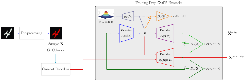
Figure D.1: Training the deep variational $\mathsf{GenPF}$ model on Colored-MNIST dataset, employing the learning scenario ‘End-to-End Raw Data Scratch Learning’.

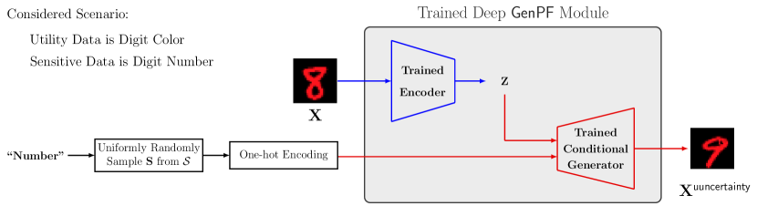
Figure D.2: Evaluating the performance of the deep variational GenPF model, trained on the Colored-MNIST dataset, with the digit number as the sensitive attribute and the digit color as the useful data.

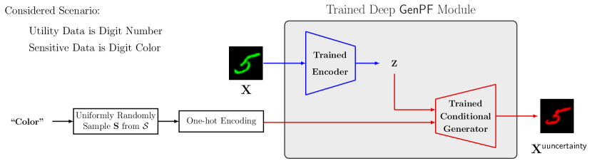
Figure D.3: Evaluating the performance of the deep variational GenPF model, trained on the Colored-MNIST dataset, with the digit color as the sensitive attribute and the digit number as the useful data.

Figure D.4: Qualitative evaluation of privacy-preserving synthetic samples $\mathbf{X}^{\texttt{uncertainty}}$ generated by the conditional generator $g_{\bm{\varphi}}$, using a custom Colored-MNIST dataset, where the sensitive attribute under consideration is the digit color. The setting is defined with $d_{\mathbf{z}}=8$. For scenario (a), the color probabilities are set as $P_{S}(\mathsf{Red})=\frac{1}{2}$, $P_{S}(\mathsf{Green})=\frac{1}{6}$, and $P_{S}(\mathsf{Blue})=\frac{1}{3}$. In scenario (b), all probabilities are equal with $P_{S}(\mathsf{Red})=P_{S}(\mathsf{Green})=P_{S}(\mathsf{Blue})=\frac{1}{3}$.

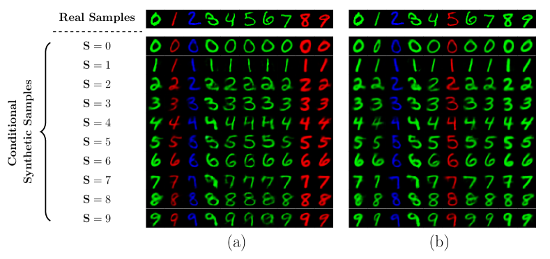
Figure D.5: Qualitative evaluation of privacy-preserving synthetic samples $\mathbf{X}^{\texttt{uncertainty}}$ generated by the conditional generator $g_{\bm{\varphi}}$, using a custom Colored-MNIST dataset, where the sensitive attribute under consideration is the digit number. The setting is defined with $d_{\mathbf{z}}=8$. For scenario (a), the color probabilities are set as $P_{S}(\mathsf{Red})=\frac{1}{2}$, $P_{S}(\mathsf{Green})=\frac{1}{6}$, and $P_{S}(\mathsf{Blue})=\frac{1}{3}$. In scenario (b), all probabilities are equal with $P_{S}(\mathsf{Red})=P_{S}(\mathsf{Green})=P_{S}(\mathsf{Blue})=\frac{1}{3}$.

References

- Abadi et al. (2016) Martin Abadi, Andy Chu, Ian Goodfellow, H Brendan McMahan, Ilya Mironov, Kunal Talwar, and Li Zhang. Deep learning with differential privacy. In Proceedings of the 2016 ACM SIGSAC conference on computer and communications security, pages 308–318, 2016.
- Abdullahi et al. (2024) Sani M Abdullahi, Shuifa Sun, Beng Wang, Ning Wei, and Hongxia Wang. Biometric template attacks and recent protection mechanisms: A survey. Information Fusion, 103:102144, 2024.
- Abdullakutty et al. (2021) Faseela Abdullakutty, Eyad Elyan, and Pamela Johnston. A review of state-of-the-art in face presentation attack detection: From early development to advanced deep learning and multi-modal fusion methods. Information fusion, 75:55–69, 2021.
- Agrawal and Srikant (2000) Rakesh Agrawal and Ramakrishnan Srikant. Privacy-preserving data mining. In Proceedings of the 2000 ACM SIGMOD international conference on Management of data, pages 439–450, 2000.
- Alemi et al. (2016) Alexander A Alemi, Ian Fischer, Joshua V Dillon, and Kevin Murphy. Deep variational information bottleneck. arXiv preprint arXiv:1612.00410, 2016.
- Ali and Silvey (1966) Syed Mumtaz Ali and Samuel D Silvey. A general class of coefficients of divergence of one distribution from another. Journal of the Royal Statistical Society: Series B (Methodological), 28(1):131–142, 1966.
- Alzantot et al. (2019) Moustafa Alzantot, Yash Sharma, Supriyo Chakraborty, Huan Zhang, Cho-Jui Hsieh, and Mani B Srivastava. Genattack: Practical black-box attacks with gradient-free optimization. In Proceedings of the genetic and evolutionary computation conference, pages 1111–1119, 2019.
- Amjad and Geiger (2019) Rana Ali Amjad and Bernhard Claus Geiger. Learning representations for neural network-based classification using the information bottleneck principle. IEEE Transactions on Pattern Analysis and Machine Intelligence, 2019.
- Amos et al. (2016) Brandon Amos, Bartosz Ludwiczuk, and Mahadev Satyanarayanan. Openface: A general-purpose face recognition library with mobile applications. Technical report, CMU-CS-16-118, CMU School of Computer Science, 2016.
- Arimoto (1977) Suguru Arimoto. Information measures and capacity of order for discrete memoryless channels. Topics in Information Theory, 16:41–52, 1977.
- Asoodeh and Calmon (2020) Shahab Asoodeh and Flavio P Calmon. Bottleneck problems: An information and estimation-theoretic view. Entropy, 22(11):1325, 2020.
- Asoodeh et al. (2014) Shahab Asoodeh, Fady Alajaji, and Tamás Linder. Notes on information-theoretic privacy. In 52nd Annual Allerton Conference on Communication, Control, and Computing, pages 1272–1278. IEEE, 2014.
- Asoodeh et al. (2016) Shahab Asoodeh, Mario Diaz, Fady Alajaji, and Tamás Linder. Information extraction under privacy constraints. Information, 7(1):15, 2016.
- Asoodeh et al. (2018) Shahab Asoodeh, Mario Diaz, Fady Alajaji, and Tamás Linder. Estimation efficiency under privacy constraints. IEEE Transactions on Information Theory, 65(3):1512–1534, 2018.
- Asoodeh et al. (2021) Shahab Asoodeh, Maryam Aliakbarpour, and Flavio P Calmon. Local differential privacy is equivalent to contraction of an -divergence. In 2021 IEEE International Symposium on Information Theory (ISIT), pages 545–550. IEEE, 2021.
- Atashin et al. (2021) Amir Ahooye Atashin, Behrooz Razeghi, Deniz Gündüz, and Slava Voloshynovskiy. Variational leakage: The role of information complexity in privacy leakage. In 3rd ACM Workshop on Wireless Security and Machine Learning, pages 91–96, 2021.
- Backes et al. (2016) Michael Backes, Pascal Berrang, Anna Hecksteden, Mathias Humbert, Andreas Keller, and Tim Meyer. Privacy in epigenetics: Temporal linkability of MicroRNA expression profiles. In 25th USENIX security symposium (USENIX Security 16), pages 1223–1240, 2016.
- Bang et al. (2019) Seojin Bang, Pengtao Xie, Heewook Lee, Wei Wu, and Eric Xing. Explaining a black-box using deep variational information bottleneck approach. arXiv preprint arXiv:1902.06918, 2019.
- Basciftci et al. (2016) Yuksel Ozan Basciftci, Ye Wang, and Prakash Ishwar. On privacy-utility tradeoffs for constrained data release mechanisms. In Information Theory and Applications Workshop (ITA), pages 1–6. IEEE, 2016.
- Bassit et al. (2021) Amina Bassit, Florian Hahn, Joep Peeters, Tom Kevenaar, Raymond Veldhuis, and Andreas Peter. Fast and accurate likelihood ratio-based biometric verification secure against malicious adversaries. IEEE transactions on information forensics and security, 16:5045–5060, 2021.
- Batina et al. (2019) Lejla Batina, Shivam Bhasin, Dirmanto Jap, and Stjepan Picek. CSINN: Reverse engineering of neural network architectures through electromagnetic side channel. In 28th USENIX Security Symposium (USENIX Security 19), pages 515–532, 2019.
- Beigi and Liu (2020) Ghazaleh Beigi and Huan Liu. A survey on privacy in social media: Identification, mitigation, and applications. ACM Transactions on Data Science, 1(1):1–38, 2020.
- Belghazi et al. (2018) Mohamed Ishmael Belghazi, Aristide Baratin, Sai Rajeshwar, Sherjil Ozair, Yoshua Bengio, Aaron Courville, and Devon Hjelm. Mutual information neural estimation. In International conference on machine learning, pages 531–540. PMLR, 2018.
- Bhagoji et al. (2018) Arjun Nitin Bhagoji, Warren He, Bo Li, and Dawn Song. Practical black-box attacks on deep neural networks using efficient query mechanisms. In Proceedings of the European conference on computer vision (ECCV), pages 154–169, 2018.
- Bhowmick et al. (2018) Abhishek Bhowmick, John Duchi, Julien Freudiger, Gaurav Kapoor, and Ryan Rogers. Protection against reconstruction and its applications in private federated learning. arXiv preprint arXiv:1812.00984, 2018.
- Biggio et al. (2012) Battista Biggio, Blaine Nelson, and Pavel Laskov. Poisoning attacks against support vector machines. arXiv preprint arXiv:1206.6389, 2012.
- Biggio et al. (2015) Battista Biggio, Paolo Russu, Luca Didaci, Fabio Roli, et al. Adversarial biometric recognition: A review on biometric system security from the adversarial machine-learning perspective. IEEE Signal Processing Magazine, 32(5):31–41, 2015.
- Bishop and Nasrabadi (2006) Christopher M Bishop and Nasser M Nasrabadi. Pattern recognition and machine learning, volume 4. Springer, 2006.
- Bloch et al. (2021) Matthieu Bloch, Onur Günlü, Aylin Yener, Frédérique Oggier, H Vincent Poor, Lalitha Sankar, and Rafael F Schaefer. An overview of information-theoretic security and privacy: Metrics, limits and applications. IEEE Journal on Selected Areas in Information Theory, 2(1):5–22, 2021.
- Bober-Irizar et al. (2023) Mikel Bober-Irizar, Ilia Shumailov, Yiren Zhao, Robert Mullins, and Nicolas Papernot. Architectural backdoors in neural networks. In Proceedings of the IEEE/CVF Conference on Computer Vision and Pattern Recognition, pages 24595–24604, 2023.
- Boddeti (2018) Vishnu Naresh Boddeti. Secure face matching using fully homomorphic encryption. In 2018 IEEE 9th International Conference on Biometrics Theory, Applications and Systems (BTAS), pages 1–10. IEEE, 2018.
- Campbell et al. (2003) Katherine Campbell, Lawrence A Gordon, Martin P Loeb, and Lei Zhou. The economic cost of publicly announced information security breaches: empirical evidence from the stock market. Journal of Computer security, 11(3):431–448, 2003.
- Carlini et al. (2023) Nicholas Carlini, Matthew Jagielski, Christopher A Choquette-Choo, Daniel Paleka, Will Pearce, Hyrum Anderson, Andreas Terzis, Kurt Thomas, and Florian Tramèr. Poisoning web-scale training datasets is practical. arXiv preprint arXiv:2302.10149, 2023.
- Chandrasekaran et al. (2020) Varun Chandrasekaran, Kamalika Chaudhuri, Irene Giacomelli, Somesh Jha, and Songbai Yan. Exploring connections between active learning and model extraction. In 29th USENIX Security Symposium (USENIX Security 20), pages 1309–1326, 2020.
- Chaum (1985) David Chaum. Security without identification: Transaction systems to make big brother obsolete. Communications of the ACM, 28(10):1030–1044, 1985.
- Chaum (1981) David L Chaum. Untraceable electronic mail, return addresses, and digital pseudonyms. Communications of the ACM, 24(2):84–90, 1981.
- Chen et al. (2023) Xinquan Chen, Xitong Gao, Juanjuan Zhao, Kejiang Ye, and Cheng-Zhong Xu. Advdiffuser: Natural adversarial example synthesis with diffusion models. In Proceedings of the IEEE/CVF International Conference on Computer Vision, pages 4562–4572, 2023.
- Cramer et al. (2015) Ronald Cramer, Ivan Bjerre Damgård, et al. Secure multiparty computation. Cambridge University Press, 2015.
- Csiszár (1967) Imre Csiszár. Information-type measures of difference of probability distributions and indirect observation. studia scientiarum Mathematicarum Hungarica, 2:229–318, 1967.
- Csiszár et al. (2004) Imre Csiszár, Paul C Shields, et al. Information theory and statistics: A tutorial. Foundations and Trends® in Communications and Information Theory, 1(4):417–528, 2004.
- de Freitas and Geiger (2022) João Machado de Freitas and Bernhard C Geiger. Funck: Information funnels and bottlenecks for invariant representation learning. arXiv preprint arXiv:2211.01446, 2022.
- Deng et al. (2019a) Jiankang Deng, Jia Guo, Niannan Xue, and Stefanos Zafeiriou. Arcface: Additive angular margin loss for deep face recognition. In IEEE/CVF CVPR, 2019a. doi:10.1109/CVPR.2019.00482.
- Deng et al. (2019b) Jiankang Deng, Jia Guo, Debing Zhang, Yafeng Deng, Xiangju Lu, and Song Shi. Lightweight face recognition challenge. In IEEE/CVF ICCV Workshops, 2019b.
- Diaz et al. (2019) Mario Diaz, Hao Wang, Flavio P. Calmon, and Lalitha Sankar. On the robustness of information-theoretic privacy measures and mechanisms. IEEE Transactions on Information Theory, 66(4):1949–1978, 2019.
- Diffie and Hellman (1976) Whitfield Diffie and Martin E Hellman. New directions in cryptography. IEEE Transactions on Information Theory, 1976.
- Ding and Sadeghi (2019) Ni Ding and Parastoo Sadeghi. A submodularity-based clustering algorithm for the information bottleneck and privacy funnel. In IEEE Information Theory Workshop (ITW), pages 1–5. IEEE, 2019.
- Donsker and Varadhan (1983) Monroe D Donsker and SR Srinivasa Varadhan. Asymptotic evaluation of certain markov process expectations for large time. iv. Communications on pure and applied mathematics, 36(2):183–212, 1983.
- Du and Atallah (2001) Wenliang Du and Mikhail J Atallah. Secure multi-party computation problems and their applications: a review and open problems. In Proceedings of the 2001 workshop on New security paradigms, pages 13–22, 2001.
- Duchi (2016) John Duchi. Lecture notes for statistics 311/electrical engineering 377. URL: https://stanford. edu/class/stats311/Lectures/full notes., 2, 2016.
- Duchi et al. (2013a) John C Duchi, Michael I Jordan, and Martin J Wainwright. Local privacy, data processing inequalities, and statistical minimax rates. arXiv preprint arXiv:1302.3203, 2013a.
- Duchi et al. (2013b) John C Duchi, Michael I Jordan, and Martin J Wainwright. Local privacy and statistical minimax rates. In 2013 IEEE 54th Annual Symposium on Foundations of Computer Science, pages 429–438. IEEE, 2013b.
- Duchi et al. (2014) John C Duchi, Michael I Jordan, and Martin J Wainwright. Privacy aware learning. Journal of the ACM (JACM), 61(6):1–57, 2014.
- Duchi et al. (2018) John C Duchi, Michael I Jordan, and Martin J Wainwright. Minimax optimal procedures for locally private estimation. Journal of the American Statistical Association, 113(521):182–201, 2018.
- Dunne (1994) Robert L Dunne. Deterring unauthorized access to computers: Controlling behavior in cyberspace through a contract law paradigm. Jurimetrics J., 35:1, 1994.
- Duta et al. (2021) Ionut Cosmin Duta, Li Liu, Fan Zhu, and Ling Shao. Improved residual networks for image and video recognition. In 25th International Conference on Pattern Recognition (ICPR), pages 9415–9422. IEEE, 2021.
- Dwivedi et al. (2019) Ashutosh Dhar Dwivedi, Gautam Srivastava, Shalini Dhar, and Rajani Singh. A decentralized privacy-preserving healthcare blockchain for iot. Sensors, 19(2):326, 2019.
- Dwork et al. (2006a) Cynthia Dwork, Krishnaram Kenthapadi, Frank McSherry, Ilya Mironov, and Moni Naor. Our data, ourselves: Privacy via distributed noise generation. In Advances in Cryptology-EUROCRYPT 2006: 24th Annual International Conference on the Theory and Applications of Cryptographic Techniques, St. Petersburg, Russia, May 28-June 1, 2006. Proceedings 25, pages 486–503. Springer, 2006a.
- Dwork et al. (2006b) Cynthia Dwork, Frank McSherry, Kobbi Nissim, and Adam Smith. Calibrating noise to sensitivity in private data analysis. In Theory of Cryptography Conference, pages 265–284. Springer, 2006b.
- Dwork et al. (2014) Cynthia Dwork, Aaron Roth, et al. The algorithmic foundations of differential privacy. Foundations and Trends® in Theoretical Computer Science, 9(3–4):211–407, 2014.
- Dwork et al. (2017) Cynthia Dwork, Adam Smith, Thomas Steinke, and Jonathan Ullman. Exposed! a survey of attacks on private data. Annual Review of Statistics and Its Application, 4:61–84, 2017.
- Edwards and Storkey (2016) Harrison Edwards and Amos Storkey. Censoring representations with an adversary. In International Conference on Learning Representation (ICLR), 2016.
- Effing et al. (2011) Robin Effing, Jos Van Hillegersberg, and Theo Huibers. Social media and political participation: are facebook, twitter and youtube democratizing our political systems? In Electronic Participation: Third IFIP WG 8.5 International Conference, ePart 2011, Delft, The Netherlands, August 29–September 1, 2011. Proceedings 3, pages 25–35. Springer, 2011.
- El Emam et al. (2011) Khaled El Emam, Elizabeth Jonker, Luk Arbuckle, and Bradley Malin. A systematic review of re-identification attacks on health data. PloS one, 6(12):e28071, 2011.
- Evfimievski et al. (2003) Alexandre Evfimievski, Johannes Gehrke, and Ramakrishnan Srikant. Limiting privacy breaches in privacy preserving data mining. In 22th ACM SIGMOD-SIGACT-SIGART symposium on Principles of database systems, pages 211–222. ACM, 2003.
- Federici et al. (2020) Marco Federici, Anjan Dutta, Patrick Forré, Nate Kushman, and Zeynep Akata. Learning robust representations via multi-view information bottleneck. International Conference on Learning Representations (ICLR), 2020.
- Ferdowsi et al. (2020) Sohrab Ferdowsi, Behrooz Razeghi, Taras Holotyak, Flavio P Calmon, and Slava Voloshynovskiy. Privacy-preserving image sharing via sparsifying layers on convolutional groups. In IEEE International Conference on Acoustics, Speech and Signal Processing (ICASSP), pages 2797–2801. IEEE, 2020.
- Fiege et al. (1987) Uriel Fiege, Amos Fiat, and Adi Shamir. Zero knowledge proofs of identity. In Proceedings of the nineteenth annual ACM symposium on Theory of computing, pages 210–217, 1987.
- Fischer (2020) Ian Fischer. The conditional entropy bottleneck. arXiv preprint arXiv:2002.05379, 2020.
- Galbally et al. (2010) Javier Galbally, Chris McCool, Julian Fierrez, Sebastien Marcel, and Javier Ortega-Garcia. On the vulnerability of face verification systems to hill-climbing attacks. Pattern Recognition, 43(3):1027–1038, 2010.
- Goldfeld and Polyanskiy (2020) Ziv Goldfeld and Yury Polyanskiy. The information bottleneck problem and its applications in machine learning. IEEE Journal on Selected Areas in Information Theory, 2020.
- Goldreich (1998) Oded Goldreich. Secure multi-party computation. Manuscript. Preliminary version, 78(110), 1998.
- Goldreich and Oren (1994) Oded Goldreich and Yair Oren. Definitions and properties of zero-knowledge proof systems. Journal of Cryptology, 7(1):1–32, 1994.
- Gong et al. (2020) Sixue Gong, Xiaoming Liu, and Anil K Jain. Jointly de-biasing face recognition and demographic attribute estimation. In Computer Vision–ECCV 2020: 16th European Conference, Glasgow, UK, August 23–28, 2020, Proceedings, Part XXIX 16, pages 330–347. Springer, 2020.
- Grover and Mark (2017) Ted Grover and Gloria Mark. Digital footprints: Predicting personality from temporal patterns of technology use. In Proceedings of the 2017 acm international joint conference on pervasive and ubiquitous computing and proceedings of the 2017 acm international symposium on wearable computers, pages 41–44, 2017.
- Guizzo (2003) Erico Marui Guizzo. The essential message: Claude Shannon and the making of information theory. PhD thesis, Massachusetts Institute of Technology, 2003.
- Guo et al. (2019) Chuan Guo, Jacob Gardner, Yurong You, Andrew Gordon Wilson, and Kilian Weinberger. Simple black-box adversarial attacks. In International Conference on Machine Learning, pages 2484–2493. PMLR, 2019.
- Guo and Liu (2020) Junfeng Guo and Cong Liu. Practical poisoning attacks on neural networks. In Computer Vision–ECCV 2020: 16th European Conference, Glasgow, UK, August 23–28, 2020, Proceedings, Part XXVII 16, pages 142–158. Springer, 2020.
- Hafez-Kolahi and Kasaei (2019) Hassan Hafez-Kolahi and Shohreh Kasaei. Information bottleneck and its applications in deep learning. Algorithms, 3(4):5, 2019.
- Hafez-Kolahi et al. (2020) Hassan Hafez-Kolahi, Shohreh Kasaei, and Mahdiyeh Soleymani-Baghshah. Sample complexity of classification with compressed input. Neurocomputing, 2020.
- Hahn and Marcel (2022) Vedrana Krivokuća Hahn and Sébastien Marcel. Biometric template protection for neural-network-based face recognition systems: A survey of methods and evaluation techniques. IEEE Transactions on Information Forensics and Security, 18:639–666, 2022.
- Hamm (2017) Jihun Hamm. Enhancing utility and privacy with noisy minimax filters. In IEEE International Conference on Acoustics, Speech and Signal Processing (ICASSP), pages 6389–6393. IEEE, 2017.
- He et al. (2016) Kaiming He, Xiangyu Zhang, Shaoqing Ren, and Jian Sun. Deep residual learning for image recognition. In IEEE CVPR, 2016. doi:10.1109/CVPR.2016.90.
- Hellman (1976) Martin Hellman. New directions in cryptography. IEEE transactions on Information Theory, 22(6):644–654, 1976.
- Hellman (1977) Martin Hellman. An extension of the shannon theory approach to cryptography. IEEE Transactions on Information Theory, 23(3):289–294, 1977.
- Henriksen-Bulmer and Jeary (2016) Jane Henriksen-Bulmer and Sheridan Jeary. Re-identification attacks—a systematic literature review. International Journal of Information Management, 36(6):1184–1192, 2016.
- Howard et al. (2017) Andrew G Howard, Menglong Zhu, Bo Chen, Dmitry Kalenichenko, Weijun Wang, Tobias Weyand, Marco Andreetto, and Hartwig Adam. Mobilenets: Efficient convolutional neural networks for mobile vision applications. arXiv preprint arXiv:1704.04861, 2017.
- Hsu et al. (2019) Hsiang Hsu, Shahab Asoodeh, Flávio P. Calmon, and Nadia Fawaz. Information-theoretic privacy watchdogs. In IEEE International Symposium on Information Theory (ISIT). IEEE, 2019.
- Hsu et al. (2020) Hsiang Hsu, Shahab Asoodeh, and Flavio Calmon. Obfuscation via information density estimation. In International Conference on Artificial Intelligence and Statistics (AISTATS), pages 906–917. PMLR, 2020.
- Hsu et al. (2021) Hsiang Hsu, Natalia Martinez, Martin Bertran, Guillermo Sapiro, and Flavio P Calmon. A survey on statistical, information, and estimation—theoretic views on privacy. IEEE BITS the Information Theory Magazine, 1(1):45–56, 2021.
- Hu et al. (2019) Jie Hu, Rongrong Ji, ShengChuan Zhang, Xiaoshuai Sun, Qixiang Ye, Chia-Wen Lin, and Qi Tian. Information competing process for learning diversified representations. In Advances in Neural Information Processing Systems, pages 2175–2186, 2019.
- Hu et al. (2022) Pingyi Hu, Zihan Wang, Ruoxi Sun, Hu Wang, and Minhui Xue. M 4 i: Multi-modal models membership inference. Advances in Neural Information Processing Systems, 35:1867–1882, 2022.
- Huang et al. (2017) Chong Huang, Peter Kairouz, Xiao Chen, Lalitha Sankar, and Ram Rajagopal. Context-aware generative adversarial privacy. Entropy, 19(12):656, 2017.
- Huang et al. (2018) Chong Huang, Peter Kairouz, Xiao Chen, Lalitha Sankar, and Ram Rajagopal. Generative adversarial privacy. arXiv preprint arXiv:1807.05306, 2018.
- Huang et al. (2008) Gary B Huang, Marwan Mattar, Tamara Berg, and Eric Learned-Miller. Labeled faces in the wild: A database forstudying face recognition in unconstrained environments. In Workshop on faces in’Real-Life’Images: detection, alignment, and recognition, 2008.
- Huang and Gamal (2024) Teng-Hui Huang and Hesham El Gamal. An efficient difference-of-convex solver for privacy funnel. arXiv preprint arXiv:2403.04778, 2024.
- Ilyas et al. (2018) Andrew Ilyas, Logan Engstrom, Anish Athalye, and Jessy Lin. Black-box adversarial attacks with limited queries and information. In International conference on machine learning, pages 2137–2146. PMLR, 2018.
- ISO/IEC 24745:2022 (E) ISO/IEC 24745:2022(E). ISO/IEC 24745: 2022(E) Information technologyy, cybersecurity and privacy protection – Biometric Information Protection, Feb 2022. URL https://www.iso.org/standard/75302.html.
- Issa et al. (2019) Ibrahim Issa, Aaron B Wagner, and Sudeep Kamath. An operational approach to information leakage. IEEE Transactions on Information Theory, 66(3):1625–1657, 2019.
- James et al. (2013) Gareth James, Daniela Witten, Trevor Hastie, Robert Tibshirani, et al. An introduction to statistical learning, volume 112. Springer, 2013.
- Jin et al. (2004) Andrew Teoh Beng Jin, David Ngo Chek Ling, and Alwyn Goh. Biohashing: two factor authentication featuring fingerprint data and tokenised random number. Pattern Recognition, 37(11):2245–2255, 2004.
- Jin et al. (2017) Zhe Jin, Jung Yeon Hwang, Yen-Lung Lai, Soohyung Kim, and Andrew Beng Jin Teoh. Ranking-based locality sensitive hashing-enabled cancelable biometrics: Index-of-max hashing. IEEE Transactions on Information Forensics and Security, 13(2):393–407, 2017.
- Juels and Sudan (2006) Ari Juels and Madhu Sudan. A fuzzy vault scheme. Designs, Codes and Cryptography, 38(2):237–257, 2006.
- Juels and Wattenberg (1999) Ari Juels and Martin Wattenberg. A fuzzy commitment scheme. In Proceedings of the 6th ACM Conference on Computer and Communications Security, pages 28–36, 1999.
- Juvekar et al. (2018) Chiraag Juvekar, Vinod Vaikuntanathan, and Anantha Chandrakasan. GAZELLE: A low latency framework for secure neural network inference. In 27th USENIX Security Symposium (USENIX Security 18), pages 1651–1669, 2018.
- Kairouz et al. (2021) Peter Kairouz, H Brendan McMahan, Brendan Avent, Aurélien Bellet, Mehdi Bennis, Arjun Nitin Bhagoji, Kallista Bonawitz, Zachary Charles, Graham Cormode, Rachel Cummings, et al. Advances and open problems in federated learning. Foundations and Trends® in Machine Learning, 14(1–2):1–210, 2021.
- Kaissis et al. (2020) Georgios A Kaissis, Marcus R Makowski, Daniel Rückert, and Rickmer F Braren. Secure, privacy-preserving and federated machine learning in medical imaging. Nature Machine Intelligence, 2(6):305–311, 2020.
- Kalantari et al. (2017) Kousha Kalantari, Lalitha Sankar, and Oliver Kosut. On information-theoretic privacy with general distortion cost functions. In IEEE International Symposium on Information Theory (ISIT), pages 2865–2869. IEEE, 2017.
- Kamat et al. (2009) Pandurang Kamat, Wenyuan Xu, Wade Trappe, and Yanyong Zhang. Temporal privacy in wireless sensor networks: Theory and practice. ACM Transactions on Sensor Networks (TOSN), 5(4):1–24, 2009.
- Kantorovich (1942) Leonid Kantorovich. On the transfer of masses (in russian). In Doklady Akademii Nauk, volume 37, pages 227––229, 1942.
- Karkkainen and Joo (2021) Kimmo Karkkainen and Jungseock Joo. Fairface: Face attribute dataset for balanced race, gender, and age for bias measurement and mitigation. In IEEE/CVF Winter Conference on Applications of Computer Vision, 2021.
- Keller (2020) Marcel Keller. Mp-spdz: A versatile framework for multi-party computation. In Proceedings of the 2020 ACM SIGSAC conference on computer and communications security, pages 1575–1590, 2020.
- Kifer and Machanavajjhala (2012) Daniel Kifer and Ashwin Machanavajjhala. A rigorous and customizable framework for privacy. In 31st ACM SIGMOD-SIGACT-SIGAI symposium on Principles of Database Systems, pages 77–88. ACM, 2012.
- Kilian (1992) Joe Kilian. A note on efficient zero-knowledge proofs and arguments. In Proceedings of the twenty-fourth annual ACM symposium on Theory of computing, pages 723–732, 1992.
- Kim et al. (2022) Minchul Kim, Anil K Jain, and Xiaoming Liu. Adaface: Quality adaptive margin for face recognition. In IEEE/CVF CVPR, 2022.
- Kingma and Welling (2014) Diederik P Kingma and Max Welling. Auto-encoding variational bayes. In International Conference on Learning Representations (ICLR), 2014.
- Kirsch et al. (2020) Andreas Kirsch, Clare Lyle, and Yarin Gal. Unpacking information bottlenecks: Unifying information-theoretic objectives in deep learning. arXiv preprint arXiv:2003.12537, 2020.
- Kloukiniotis et al. (2022) A Kloukiniotis, A Papandreou, A Lalos, P Kapsalas, D-V Nguyen, and K Moustakas. Countering adversarial attacks on autonomous vehicles using denoising techniques: A review. IEEE Open Journal of Intelligent Transportation Systems, 3:61–80, 2022.
- Knott et al. (2021) Brian Knott, Shobha Venkataraman, Awni Hannun, Shubho Sengupta, Mark Ibrahim, and Laurens van der Maaten. Crypten: Secure multi-party computation meets machine learning. Advances in Neural Information Processing Systems, 34:4961–4973, 2021.
- Kolchinsky et al. (2019) Artemy Kolchinsky, Brendan D Tracey, and Steven Van Kuyk. Caveats for information bottleneck in deterministic scenarios. In International Conference on Learning Representations (ICLR), 2019.
- Kurri et al. (2023) Gowtham R Kurri, Lalitha Sankar, and Oliver Kosut. An operational approach to information leakage via generalized gain functions. IEEE Transactions on Information Theory, 2023.
- Lample et al. (2017) Guillaume Lample, Neil Zeghidour, Nicolas Usunier, Antoine Bordes, Ludovic DENOYER, et al. Fader networks: Manipulating images by sliding attributes. In Advances in Neural Information Processing Systems, pages 5963–5972, 2017.
- Layne et al. (2012) Ryan Layne, Timothy M Hospedales, Shaogang Gong, and Q Mary. Person re-identification by attributes. In Bmvc, volume 2, page 8, 2012.
- Leong et al. (2020) Shu-Min Leong, Raphaël C-W Phan, Vishnu Monn Baskaran, and Chee-Pun Ooi. Privacy-preserving facial recognition based on temporal features. Applied Soft Computing, 96:106662, 2020.
- Li et al. (2007) Ninghui Li, Tiancheng Li, and Suresh Venkatasubramanian. t-closeness: Privacy beyond k-anonymity and l-diversity. In IEEE 23rd International Conference on Data Engineering (ICDE), pages 106–115. IEEE, 2007.
- Li et al. (2023) Wenhao Li, Xiao-Yu Zhang, Huaifeng Bao, Binbin Yang, Zhaoxuan Li, Haichao Shi, and Qiang Wang. Prism: Real-time privacy protection against temporal network traffic analyzers. IEEE Transactions on Information Forensics and Security, 2023.
- Li et al. (2022) Zhiheng Li, Anthony Hoogs, and Chenliang Xu. Discover and mitigate unknown biases with debiasing alternate networks. In European Conference on Computer Vision, pages 270–288. Springer, 2022.
- Liao et al. (2018) Jiachun Liao, Oliver Kosut, Lalitha Sankar, and Flavio P. Calmon. Privacy under hard distortion constraints. In IEEE Information Theory Workshop (ITW), pages 1–5. IEEE, 2018.
- Liao et al. (2019) Jiachun Liao, Oliver Kosut, Lalitha Sankar, and Flavio P. Calmon. Tunable measures for information leakage and applications to privacy-utility tradeoffs. IEEE Transactions on Information Theory, 65(12):8043–8066, 2019.
- Liu et al. (2021) Ajian Liu, Zichang Tan, Jun Wan, Yanyan Liang, Zhen Lei, Guodong Guo, and Stan Z Li. Face anti-spoofing via adversarial cross-modality translation. IEEE Transactions on Information Forensics and Security, 16:2759–2772, 2021.
- Liu et al. (2017) Weiyang Liu, Yandong Wen, Zhiding Yu, Ming Li, Bhiksha Raj, and Le Song. Sphereface: Deep hypersphere embedding for face recognition. In Proceedings of the IEEE conference on computer vision and pattern recognition, pages 212–220, 2017.
- Liu et al. (2016) Yanpei Liu, Xinyun Chen, Chang Liu, and Dawn Song. Delving into transferable adversarial examples and black-box attacks. arXiv preprint arXiv:1611.02770, 2016.
- Lowe (1999) David G Lowe. Object recognition from local scale-invariant features. In 7th IEEE international conference on computer vision, volume 2, pages 1150–1157. IEEE, 1999.
- Lu et al. (2002) Chun Shien Lu, Hong-Yuan Liao, and Martin Kutter. Denoising and copy attacks resilient watermarking by exploiting prior knowledge at detector. IEEE Transactions on Image Processing, 11(3):280–292, 2002.
- Maaten and Hinton (2008) Laurens van der Maaten and Geoffrey Hinton. Visualizing data using t-sne. Journal of machine learning research, 9(Nov):2579–2605, 2008.
- Machanavajjhala et al. (2006) Ashwin Machanavajjhala, Johannes Gehrke, Daniel Kifer, and Muthuramakrishnan Venkitasubramaniam. l-diversity: Privacy beyond k-anonymity. In Data Engineering, 2006. ICDE’06. Proceedings of the 22nd International Conference on, pages 24–24. IEEE, 2006.
- Machanavajjhala et al. (2008) Ashwin Machanavajjhala, Daniel Kifer, John Abowd, Johannes Gehrke, and Lars Vilhuber. Privacy: Theory meets practice on the map. In 2008 IEEE 24th international conference on data engineering, pages 277–286. IEEE, 2008.
- Mai et al. (2020) Guangcan Mai, Kai Cao, Xiangyuan Lan, and Pong C Yuen. Secureface: Face template protection. IEEE Transactions on Information Forensics and security, 16:262–277, 2020.
- Maithili et al. (2018) K Maithili, V Vinothkumar, and P Latha. Analyzing the security mechanisms to prevent unauthorized access in cloud and network security. Journal of Computational and Theoretical Nanoscience, 15(6-7):2059–2063, 2018.
- Makhdoumi and Fawaz (2013) Ali Makhdoumi and Nadia Fawaz. Privacy-utility tradeoff under statistical uncertainty. In 51st Annual Allerton Conference on Communication, Control, and Computing, pages 1627–1634. IEEE, 2013.
- Makhdoumi et al. (2014) Ali Makhdoumi, Salman Salamatian, Nadia Fawaz, and Muriel Médard. From the information bottleneck to the privacy funnel. In IEEE Information Theory Workshop (ITW), pages 501–505. IEEE, 2014.
- Marcel et al. (2023) Sébastien Marcel, Julian Fierrez, and Nicholas Evans. Handbook of Biometric Anti-Spoofing: Presentation Attack Detection and Vulnerability Assessment. Springer, 2023.
- Maze et al. (2018) Brianna Maze, Jocelyn Adams, James A. Duncan, Nathan Kalka, Tim Miller, Charles Otto, Anil K. Jain, W. Tyler Niggel, Janet Anderson, Jordan Cheney, and Patrick Grother. Iarpa janus benchmark - c: Face dataset and protocol. In International Conference on Biometrics (ICB), pages 158–165, 2018. doi:10.1109/ICB2018.2018.00033.
- McMahan et al. (2017) Brendan McMahan, Eider Moore, Daniel Ramage, Seth Hampson, and Blaise Aguera y Arcas. Communication-efficient learning of deep networks from decentralized data. In Artificial intelligence and statistics, pages 1273–1282. PMLR, 2017.
- Melzi et al. (2023) Pietro Melzi, Hatef Otroshi Shahreza, Christian Rathgeb, Ruben Tolosana, Ruben Vera-Rodriguez, Julian Fierrez, Sébastien Marcel, and Christoph Busch. Multi-ive: Privacy enhancement of multiple soft-biometrics in face embeddings. In Proceedings of the IEEE/CVF Winter Conference on Applications of Computer Vision, pages 323–331, 2023.
- Mendes and Vilela (2017) Ricardo Mendes and João P Vilela. Privacy-preserving data mining: methods, metrics, and applications. IEEE Access, 5:10562–10582, 2017.
- Micali and Rogaway (1992) Silvio Micali and Phillip Rogaway. Secure computation. Springer, 1992.
- Milne et al. (2017) George R Milne, George Pettinico, Fatima M Hajjat, and Ereni Markos. Information sensitivity typology: Mapping the degree and type of risk consumers perceive in personal data sharing. Journal of Consumer Affairs, 51(1):133–161, 2017.
- Mironov (2017) Ilya Mironov. Rényi differential privacy. In 2017 IEEE 30th computer security foundations symposium (CSF), pages 263–275. IEEE, 2017.
- Mo et al. (2022) Fan Mo, Zahra Tarkhani, and Hamed Haddadi. Sok: machine learning with confidential computing. arXiv preprint arXiv:2208.10134, 2022.
- Mohammed (2012) Ishaq Azhar Mohammed. Analysis of identity and access management alternatives for a multinational information-sharing environment. INTERNATIONAL JOURNAL OF ADVANCED AND INNOVATIVE RESEARCH, 1(8):1–7, 2012.
- Mohassel and Rindal (2018) Payman Mohassel and Peter Rindal. Aby3: A mixed protocol framework for machine learning. In Proceedings of the 2018 ACM SIGSAC conference on computer and communications security, pages 35–52, 2018.
- Monge (1781) Gaspar Monge. Mémoire sur la théorie des déblais et des remblais. Histoire de l’Académie Royale des Sciences de Paris, avec les Mémoires de Mathématique et de Physique pour la même année, pages 666–704, 1781.
- Morales et al. (2020) Aythami Morales, Julian Fierrez, Ruben Vera-Rodriguez, and Ruben Tolosana. Sensitivenets: Learning agnostic representations with application to face images. IEEE Transactions on Pattern Analysis and Machine Intelligence, 43(6):2158–2164, 2020.
- Muslukhov et al. (2013) Ildar Muslukhov, Yazan Boshmaf, Cynthia Kuo, Jonathan Lester, and Konstantin Beznosov. Know your enemy: the risk of unauthorized access in smartphones by insiders. In Proceedings of the 15th international conference on Human-computer interaction with mobile devices and services, pages 271–280, 2013.
- Nandakumar and Jain (2015) Karthik Nandakumar and Anil K Jain. Biometric template protection: Bridging the performance gap between theory and practice. IEEE Signal Processing Magazine, 32(5):88–100, 2015.
- Narayanan and Shmatikov (2008) Arvind Narayanan and Vitaly Shmatikov. Robust de-anonymization of large sparse datasets. In 2008 IEEE Symposium on Security and Privacy (sp 2008), pages 111–125. IEEE, 2008.
- Neel et al. (2021) Seth Neel, Aaron Roth, and Saeed Sharifi-Malvajerdi. Descent-to-delete: Gradient-based methods for machine unlearning. In Algorithmic Learning Theory, pages 931–962. PMLR, 2021.
- Nguyen et al. (2010) XuanLong Nguyen, Martin J Wainwright, and Michael I Jordan. Estimating divergence functionals and the likelihood ratio by convex risk minimization. IEEE Transactions on Information Theory, 56(11):5847–5861, 2010.
- Orekondy et al. (2017) Tribhuvanesh Orekondy, Bernt Schiele, and Mario Fritz. Towards a visual privacy advisor: Understanding and predicting privacy risks in images. In Proceedings of the IEEE international conference on computer vision, pages 3686–3695, 2017.
- Oseni et al. (2021) Ayodeji Oseni, Nour Moustafa, Helge Janicke, Peng Liu, Zahir Tari, and Athanasios Vasilakos. Security and privacy for artificial intelligence: Opportunities and challenges. arXiv preprint arXiv:2102.04661, 2021.
- Osia et al. (2018) Seyed Ali Osia, Ali Taheri, Ali Shahin Shamsabadi, Kleomenis Katevas, Hamed Haddadi, and Hamid R Rabiee. Deep private-feature extraction. IEEE Transactions on Knowledge and Data Engineering, 32(1):54–66, 2018.
- O’reilly et al. (2018) Michelle O’reilly, Nisha Dogra, Natasha Whiteman, Jason Hughes, Seyda Eruyar, and Paul Reilly. Is social media bad for mental health and wellbeing? exploring the perspectives of adolescents. Clinical child psychology and psychiatry, 23(4):601–613, 2018.
- P. Calmon (2015) Flavio P. Calmon. Information-theoretic metrics for security and privacy. PhD thesis, Massachusetts Institute of Technology, Department of Electrical Engineering …, 2015.
- P. Calmon and Fawaz (2012) Flavio P. Calmon and Nadia Fawaz. Privacy against statistical inference. In 50th Annual Allerton Conference on Communication, Control, and Computing, pages 1401–1408. IEEE, 2012.
- P. Calmon et al. (2013) Flavio P. Calmon, Mayank Varia, Muriel Médard, Mark M Christiansen, Ken R Duffy, and Stefano Tessaro. Bounds on inference. In 51st Annual Allerton Conference on Communication, Control, and Computing, pages 567–574. IEEE, 2013.
- P. Calmon et al. (2015) Flavio P. Calmon, Ali Makhdoumi, and Muriel Médard. Fundamental limits of perfect privacy. In IEEE International Symposium on Information Theory (ISIT), pages 1796–1800. IEEE, 2015.
- Papernot et al. (2017) Nicolas Papernot, Patrick McDaniel, Ian Goodfellow, Somesh Jha, Z Berkay Celik, and Ananthram Swami. Practical black-box attacks against machine learning. In Proceedings of the 2017 ACM on Asia conference on computer and communications security, pages 506–519, 2017.
- Park et al. (2021) Sungho Park, Sunhee Hwang, Dohyung Kim, and Hyeran Byun. Learning disentangled representation for fair facial attribute classification via fairness-aware information alignment. In Proceedings of the AAAI Conference on Artificial Intelligence, volume 35, pages 2403–2411, 2021.
- Peyré et al. (2019) Gabriel Peyré, Marco Cuturi, et al. Computational optimal transport: With applications to data science. Foundations and Trends® in Machine Learning, 11(5-6):355–607, 2019.
- Polyanskiy and Wu (2014) Yury Polyanskiy and Yihong Wu. Lecture notes on information theory. Lecture Notes for ECE563 (UIUC) and, 6, 2014.
- Polyanskiy et al. (2010) Yury Polyanskiy, H Vincent Poor, and Sergio Verdú. Channel coding rate in the finite blocklength regime. IEEE Transactions on Information Theory, 56(5):2307–2359, 2010.
- Porkodi et al. (2018) V Porkodi, M Sivaram, Amin Salih Mohammed, and V Manikandan. Survey on white-box attacks and solutions. Asian Journal of Computer Science and Technology, 7(3):28–32, 2018.
- Price (1982) Robert Price. E.“claude e. shannon: An interview conducted by robert price”. IEEE History Center, Interview, 423:28, 1982. URL https://ethw.org/Oral-History:Claude_E._Shannon.
- Prokofiev et al. (2018) Anton O Prokofiev, Yulia S Smirnova, and Vasiliy A Surov. A method to detect internet of things botnets. In 2018 IEEE Conference of Russian Young Researchers in Electrical and Electronic Engineering (EIConRus), pages 105–108. IEEE, 2018.
- Qi et al. (2020) Lianyong Qi, Chunhua Hu, Xuyun Zhang, Mohammad R Khosravi, Suraj Sharma, Shaoning Pang, and Tian Wang. Privacy-aware data fusion and prediction with spatial-temporal context for smart city industrial environment. IEEE Transactions on Industrial Informatics, 17(6):4159–4167, 2020.
- Rahmati et al. (2020) Ali Rahmati, Seyed-Mohsen Moosavi-Dezfooli, Pascal Frossard, and Huaiyu Dai. Geoda: a geometric framework for black-box adversarial attacks. In Proceedings of the IEEE/CVF conference on computer vision and pattern recognition, pages 8446–8455, 2020.
- Ramirez et al. (2022) Miguel A Ramirez, Song-Kyoo Kim, Hussam Al Hamadi, Ernesto Damiani, Young-Ji Byon, Tae-Yeon Kim, Chung-Suk Cho, and Chan Yeob Yeun. Poisoning attacks and defenses on artificial intelligence: A survey. arXiv preprint arXiv:2202.10276, 2022.
- Rassouli and Gündüz (2018) Borzoo Rassouli and Deniz Gündüz. On perfect privacy. In IEEE International Symposium on Information Theory (ISIT), pages 2551–2555. IEEE, 2018.
- Rassouli and Gündüz (2019) Borzoo Rassouli and Deniz Gündüz. Optimal utility-privacy trade-off with total variation distance as a privacy measure. IEEE Transactions on Information Forensics and Security, 15:594–603, 2019.
- Rassouli et al. (2018) Borzoo Rassouli, Fernando Rosas, and Deniz Gündüz. Latent feature disclosure under perfect sample privacy. In IEEE International Workshop on Information Forensics and Security (WIFS), pages 1–7. IEEE, 2018.
- Rassouli et al. (2019) Borzoo Rassouli, Fernando E Rosas, and Deniz Gündüz. Data disclosure under perfect sample privacy. IEEE Transactions on Information Forensics and Security, 2019.
- Rathgeb et al. (2022) Christian Rathgeb, Johannes Merkle, Johanna Scholz, Benjamin Tams, and Vanessa Nesterowicz. Deep face fuzzy vault: Implementation and performance. Computers & Security, 113:102539, 2022.
- Razeghi (2023) Behrooz Razeghi. Bottlenecks CLUB: Unifying information-theoretic trade-offs among complexity, leakage, and utility. PhD thesis, University of Geneva, Department of Computer Science, 2023. DOI: 10.13097/archive-ouverte/unige:174561.
- Razeghi et al. (2017) Behrooz Razeghi, Slava Voloshynovskiy, Dimche Kostadinov, and Olga Taran. Privacy preserving identification using sparse approximation with ambiguization. In IEEE International Workshop on Information Forensics and Security (WIFS), pages 1–6, Rennes, France, December 2017.
- Razeghi et al. (2018) Behrooz Razeghi, Slava Voloshynovskiy, Sohrab Ferdowsi, and Dimche Kostadinov. Privacy-preserving identification via layered sparse code design: Distributed servers and multiple access authorization. In 26th European Signal Processing Conference (EUSIPCO), pages 2578–2582. IEEE, 2018.
- Razeghi et al. (2020) Behrooz Razeghi, Flavio P. Calmon, Deniz Gündüz, and Slava Voloshynovskiy. On perfect obfuscation: Local information geometry analysis. In IEEE International Workshop on Information Forensics and Security (WIFS), pages 1–6, 2020.
- Razeghi et al. (2023) Behrooz Razeghi, Flavio P Calmon, Deniz Gunduz, and Slava Voloshynovskiy. Bottlenecks club: Unifying information-theoretic trade-offs among complexity, leakage, and utility. IEEE Transactions on Information Forensics and Security, 18:2060–2075, 2023.
- Razeghi et al. (2024) Behrooz Razeghi, Parsa Rahimi, and Sébastien Marcel. Deep variational privacy funnel: General modeling with applications in face recognition. In IEEE International Conference on Acoustics, Speech and Signal Processing (ICASSP), 2024. URL https://arxiv.org/pdf/2401.14792.
- Rebollo-Monedero et al. (2009) David Rebollo-Monedero, Jordi Forne, and Josep Domingo-Ferrer. From t-closeness-like privacy to postrandomization via information theory. IEEE Transactions on Knowledge and Data Engineering, 22(11):1623–1636, 2009.
- Reed (1973) Irving S Reed. Information theory and privacy in data banks. In National Computer Conference and Exposition, pages 581–587. ACM, 1973.
- Rényi (1959) Alfréd Rényi. On measures of dependence. Acta mathematica hungarica, 10(3-4):441–451, 1959.
- Rényi (1961) Alfréd Rényi. On measures of entropy and information. In Proceedings of the Fourth Berkeley Symposium on Mathematical Statistics and Probability, Volume 1: Contributions to the Theory of Statistics, volume 4, pages 547–562. University of California Press, 1961.
- Rezaeifar et al. (2019) Shideh Rezaeifar, Behrooz Razeghi, Olga Taran, Taras Holotyak, and Slava Voloshynovskiy. Reconstruction of privacy-sensitive data from protected templates. In IEEE International Conference on Image Processing (ICIP), Taipei, Taiwan, September 2019.
- Ricanek and Tesafaye (2006) K. Ricanek and T. Tesafaye. Morph: a longitudinal image database of normal adult age-progression. In International Conference on Automatic Face and Gesture Recognition, 2006. doi:10.1109/FGR.2006.78.
- Sablayrolles et al. (2019) Alexandre Sablayrolles, Matthijs Douze, Cordelia Schmid, Yann Ollivier, and Hervé Jégou. White-box vs black-box: Bayes optimal strategies for membership inference. In International Conference on Machine Learning, pages 5558–5567. PMLR, 2019.
- Sabt et al. (2015) Mohamed Sabt, Mohammed Achemlal, and Abdelmadjid Bouabdallah. Trusted execution environment: what it is, and what it is not. In 2015 IEEE Trustcom/BigDataSE/Ispa, volume 1, pages 57–64. IEEE, 2015.
- Saeidian et al. (2021) Sara Saeidian, Giulia Cervia, Tobias J Oechtering, and Mikael Skoglund. Quantifying membership privacy via information leakage. IEEE Transactions on Information Forensics and Security, 16:3096–3108, 2021.
- Saeidian et al. (2023) Sara Saeidian, Giulia Cervia, Tobias J Oechtering, and Mikael Skoglund. Pointwise maximal leakage. IEEE Transactions on Information Theory, 2023.
- Salamatian et al. (2015) Salman Salamatian, Amy Zhang, Flavio P. Calmon, Sandilya Bhamidipati, Nadia Fawaz, Branislav Kveton, Pedro Oliveira, and Nina Taft. Managing your private and public data: Bringing down inference attacks against your privacy. IEEE Journal of Selected Topics in Signal Processing, 9(7):1240–1255, 2015.
- Sandhya and Prasad (2017) Mulagala Sandhya and Munaga VNK Prasad. Biometric template protection: A systematic literature review of approaches and modalities. In Biometric Security and Privacy, pages 323–370. Springer, 2017.
- Sankar et al. (2013) Lalitha Sankar, S Raj Rajagopalan, and H Vincent Poor. Utility-privacy tradeoffs in databases: An information-theoretic approach. IEEE Transactions on Information Forensics and Security (TIFS), 8(6):838–852, 2013.
- Schroff et al. (2015) Florian Schroff, Dmitry Kalenichenko, and James Philbin. Facenet: A unified embedding for face recognition and clustering. In Proceedings of the IEEE conference on computer vision and pattern recognition, pages 815–823, 2015.
- Séjourné et al. (2023) Thibault Séjourné, Gabriel Peyré, and François-Xavier Vialard. Unbalanced optimal transport, from theory to numerics. Handbook of Numerical Analysis, 24:407–471, 2023.
- Shahreza and Marcel (2023a) Hatef Otroshi Shahreza and Sébastien Marcel. Face reconstruction from facial templates by learning latent space of a generator network. In Thirty-seventh Conference on Neural Information Processing Systems, 2023a.
- Shahreza and Marcel (2023b) Hatef Otroshi Shahreza and Sébastien Marcel. Comprehensive vulnerability evaluation of face recognition systems to template inversion attacks via 3d face reconstruction. IEEE Transactions on Pattern Analysis and Machine Intelligence, 2023b.
- Shahreza et al. (2022) Hatef Otroshi Shahreza, Christian Rathgeb, Dailé Osorio-Roig, Vedrana Krivokuća Hahn, Sébastien Marcel, and Christoph Busch. Hybrid protection of biometric templates by combining homomorphic encryption and cancelable biometrics. In 2022 IEEE International Joint Conference on Biometrics (IJCB), pages 1–10. IEEE, 2022.
- Shahreza et al. (2023a) Hatef Otroshi Shahreza, Vedrana Krivokuća Hahn, and Sébastien Marcel. Mlp-hash: Protecting face templates via hashing of randomized multi-layer perceptron. In 2023 31st European Signal Processing Conference (EUSIPCO), pages 605–609. IEEE, 2023a.
- Shahreza et al. (2023b) Hatef Otroshi Shahreza, Yanina Y Shkel, and Sébastien Marcel. Measuring linkability of protected biometric templates using maximal leakage. IEEE Transactions on Information Forensics and Security, 2023b.
- Shannon (1949) Claude E Shannon. Communication theory of secrecy systems. The Bell system technical journal, 28(4):656–715, 1949.
- Sharma and Warsi (2013) Naresh Sharma and Naqueeb Ahmad Warsi. Fundamental bound on the reliability of quantum information transmission. Physical review letters, 110(8):080501, 2013.
- Shiri et al. (2023) Isaac Shiri, Behrooz Razeghi, Alireza Vafaei Sadr, Mehdi Amini, Yazdan Salimi, Sohrab Ferdowsi, Peter Boor, Deniz Gündüz, Slava Voloshynovskiy, and Habib Zaidi. Multi-institutional pet/ct image segmentation using federated deep transformer learning. Computer Methods and Programs in Biomedicine, 240:107706, 2023.
- Shiri et al. (2024) Isaac Shiri, Behrooz Razeghi, Sohrab Ferdowsi, Yazdan Salimi, Deniz Gündüz, Douglas Teodoro, Slava Voloshynovskiy, and Habib Zaidi. Primis: Privacy-preserving medical image sharing via deep sparsifying transform learning with obfuscation. Journal of biomedical informatics, 150:104583, 2024.
- Shokri and Shmatikov (2015) Reza Shokri and Vitaly Shmatikov. Privacy-preserving deep learning. In 22nd ACM SIGSAC Conference on Computer and Communications Security, pages 1310–1321, 2015.
- Shokri et al. (2017) Reza Shokri, Marco Stronati, Congzheng Song, and Vitaly Shmatikov. Membership inference attacks against machine learning models. In 2017 IEEE symposium on security and privacy (SP), pages 3–18. IEEE, 2017.
- Simonyan and Zisserman (2014) Karen Simonyan and Andrew Zisserman. Very deep convolutional networks for large-scale image recognition. arXiv preprint arXiv:1409.1556, 2014.
- Sloan and Warner (2017) Robert Sloan and Richard Warner. Unauthorized access: The crisis in online privacy and security. Taylor & Francis, 2017.
- Smith et al. (2011) H Jeff Smith, Tamara Dinev, and Heng Xu. Information privacy research: an interdisciplinary review. MIS quarterly, pages 989–1015, 2011.
- Solove (2002) Daniel J Solove. Conceptualizing privacy. California law review, pages 1087–1155, 2002.
- Solove (2005) Daniel J Solove. A taxonomy of privacy. U. Pa. l. Rev., 154:477, 2005.
- Solove (2010) Daniel J Solove. Understanding privacy. Harvard university press, 2010.
- Solove (2024) Daniel J Solove. Artificial intelligence and privacy. Available at SSRN, 2024.
- Song et al. (2019) Liwei Song, Reza Shokri, and Prateek Mittal. Privacy risks of securing machine learning models against adversarial examples. In Proceedings of the 2019 ACM SIGSAC Conference on Computer and Communications Security, pages 241–257, 2019.
- Sreekumar and Gündüz (2019) Sreejith Sreekumar and Deniz Gündüz. Optimal privacy-utility trade-off under a rate constraint. In IEEE International Symposium on Information Theory (ISIT), pages 2159–2163. IEEE, 2019.
- Stock et al. (2022) Pierre Stock, Igor Shilov, Ilya Mironov, and Alexandre Sablayrolles. Defending against reconstruction attacks with r’enyi differential privacy. arXiv preprint arXiv:2202.07623, 2022.
- Strouse and Schwab (2017) DJ Strouse and David J Schwab. The deterministic information bottleneck. Neural computation, 29(6):1611–1630, 2017.
- Su et al. (2017) Jessica Su, Ansh Shukla, Sharad Goel, and Arvind Narayanan. De-anonymizing web browsing data with social networks. In Proceedings of the 26th international conference on world wide web, pages 1261–1269, 2017.
- Sugiyama et al. (2012) Masashi Sugiyama, Taiji Suzuki, and Takafumi Kanamori. Density-ratio matching under the Bregman divergence: A unified framework of density-ratio estimation. Annals of the Institute of Statistical Mathematics, 64(5):1009–1044, 2012.
- Suwała et al. (2024) Adrian Suwała, Bartosz Wójcik, Magdalena Proszewska, Jacek Tabor, Przemysław Spurek, and Marek Śmieja. Face identity-aware disentanglement in stylegan. In Proceedings of the IEEE/CVF Winter Conference on Applications of Computer Vision, pages 5222–5231, 2024.
- Sweeney (2000) Latanya Sweeney. Simple demographics often identify people uniquely. Health (San Francisco), 671:1–34, 2000.
- Sweeney (2002) Latanya Sweeney. k-anonymity: A model for protecting privacy. International Journal of Uncertainty, Fuzziness and Knowledge-Based Systems, 10(05):557–570, 2002.
- Taigman et al. (2014) Yaniv Taigman, Ming Yang, Marc’Aurelio Ranzato, and Lior Wolf. Deepface: Closing the gap to human-level performance in face verification. 2014 IEEE Conference on Computer Vision and Pattern Recognition, pages 1701–1708, 2014. URL https://api.semanticscholar.org/CorpusID:2814088.
- Tashiro et al. (2020) Yusuke Tashiro, Yang Song, and Stefano Ermon. Diversity can be transferred: Output diversification for white-and black-box attacks. Advances in neural information processing systems, 33:4536–4548, 2020.
- Tian et al. (2022) Zhiyi Tian, Lei Cui, Jie Liang, and Shui Yu. A comprehensive survey on poisoning attacks and countermeasures in machine learning. ACM Computing Surveys, 55(8):1–35, 2022.
- Tishby and Zaslavsky (2015) Naftali Tishby and Noga Zaslavsky. Deep learning and the information bottleneck principle. In IEEE Information Theory Workshop (ITW), pages 1–5. IEEE, 2015.
- Tishby et al. (2000) Naftali Tishby, Fernando C Pereira, and William Bialek. The information bottleneck method. In IEEE Allerton, 2000.
- Tolstikhin et al. (2018) I Tolstikhin, O Bousquet, S Gelly, and B Schölkopf. Wasserstein auto-encoders. In International Conference on Learning Representations (ICLR), 2018.
- Tramèr et al. (2016) Florian Tramèr, Fan Zhang, Ari Juels, Michael K Reiter, and Thomas Ristenpart. Stealing machine learning models via prediction APIs. In 25th USENIX security symposium (USENIX Security 16), pages 601–618, 2016.
- Tran et al. (2017) Luan Tran, Xi Yin, and Xiaoming Liu. Disentangled representation learning gan for pose-invariant face recognition. In Proceedings of the IEEE conference on computer vision and pattern recognition, pages 1415–1424, 2017.
- Tripathy et al. (2019) Ardhendu Tripathy, Ye Wang, and Prakash Ishwar. Privacy-preserving adversarial networks. In 57th Annual Allerton Conference on Communication, Control, and Computing, pages 495–505. IEEE, 2019.
- Uludag et al. (2004) Umut Uludag, Sharath Pankanti, Salil Prabhakar, and Anil K Jain. Biometric cryptosystems: issues and challenges. Proceedings of the IEEE, 92(6):948–960, 2004.
- Vaswani et al. (2023) Kapil Vaswani, Stavros Volos, Cédric Fournet, Antonio Nino Diaz, Ken Gordon, Balaji Vembu, Sam Webster, David Chisnall, Saurabh Kulkarni, Graham Cunningham, et al. Confidential computing within an AI accelerator. In 2023 USENIX Annual Technical Conference (USENIX ATC 23), pages 501–518, 2023.
- Vera et al. (2018) Matias Vera, Leonardo Rey Vega, and Pablo Piantanida. Collaborative information bottleneck. IEEE Transactions on Information Theory, 65(2):787–815, 2018.
- Villani (2008) Cédric Villani. Optimal transport: old and new, volume 338. Springer Science & Business Media, 2008.
- Voloshynovskiy et al. (2019) Slava Voloshynovskiy, Mouad Kondah, Shideh Rezaeifar, Olga Taran, Taras Holotyak, and Danilo Jimenez Rezende. Information bottleneck through variational glasses. In 4th Workshop on Bayesian Deep Learning (NeurIPS 2019), 2019.
- Voloshynovskiy et al. (2001) Sviatoslav Voloshynovskiy, Shelby Pereira, Victor Iquise, and Thierry Pun. Attack modelling: towards a second generation watermarking benchmark. Signal processing, 81(6):1177–1214, 2001.
- Voloshynovskiy et al. (2000) Sviatoslav V Voloshynovskiy, Shelby Pereira, Alexander Herrigel, Nazanin Baumgartner, and Thierry Pun. Generalized watermarking attack based on watermark estimation and perceptual remodulation. In Security and Watermarking of Multimedia Contents II, volume 3971, pages 358–370. SPIE, 2000.
- Wagner and Eckhoff (2018) Isabel Wagner and David Eckhoff. Technical privacy metrics: a systematic survey. ACM Computing Surveys (CSUR), 51(3):1–38, 2018.
- Wang and Gong (2018) Binghui Wang and Neil Zhenqiang Gong. Stealing hyperparameters in machine learning. In 2018 IEEE symposium on security and privacy (SP), pages 36–52. IEEE, 2018.
- Wang et al. (2018) Hao Wang, Yitong Wang, Zheng Zhou, Xing Ji, Dihong Gong, Jingchao Zhou, Zhifeng Li, and Wei Liu. Cosface: Large margin cosine loss for deep face recognition. In Proceedings of the IEEE conference on computer vision and pattern recognition, pages 5265–5274, 2018.
- Wang et al. (2019) Jingguo Wang, Zhe Shan, Manish Gupta, and H Raghav Rao. A longitudinal study of unauthorized access attempts on information systems: The role of opportunity contexts. MIS Quarterly, 43(2):601–622, 2019.
- Wang et al. (2022) Zhibo Wang, Jingjing Ma, Xue Wang, Jiahui Hu, Zhan Qin, and Kui Ren. Threats to training: A survey of poisoning attacks and defenses on machine learning systems. ACM Computing Surveys, 55(7):1–36, 2022.
- Wei et al. (2020) Kang Wei, Jun Li, Ming Ding, Chuan Ma, Howard H Yang, Farhad Farokhi, Shi Jin, Tony QS Quek, and H Vincent Poor. Federated learning with differential privacy: Algorithms and performance analysis. IEEE Transactions on Information Forensics and Security, 15:3454–3469, 2020.
- Winn (2007) Peter A Winn. The guilty eye: Unauthorized access, trespass and privacy. The Business Lawyer, pages 1395–1437, 2007.
- Wu et al. (2019) Tailin Wu, Ian Fischer, Isaac L Chuang, and Max Tegmark. Learnability for the information bottleneck. International Conference on Learning Representations (ICLR), 2019.
- Wyner (1975) Aaron D Wyner. The wire-tap channel. Bell system technical journal, 54(8):1355–1387, 1975.
- Xiao and Khisti (2019) Tianrui Xiao and Ashish Khisti. Maximal information leakage based privacy preserving data disclosure mechanisms. In 16th Canadian Workshop on Information Theory (CWIT), pages 1–6. IEEE, 2019.
- Xiao and Xiong (2015) Yonghui Xiao and Li Xiong. Protecting locations with differential privacy under temporal correlations. In Proceedings of the 22nd ACM SIGSAC Conference on Computer and Communications Security, pages 1298–1309, 2015.
- Yamamoto (1983) Hirosuke Yamamoto. A source coding problem for sources with additional outputs to keep secret from the receiver or wiretappers (corresp.). IEEE Transactions on Information Theory, 29(6):918–923, 1983.
- Yang et al. (2023) Haomiao Yang, Kunlan Xiang, Hongwei Li, and Rongxing Lu. A comprehensive overview of backdoor attacks in large language models within communication networks. arXiv preprint arXiv:2308.14367, 2023.
- Yao (1982) Andrew C Yao. Protocols for secure computations. In 23rd annual symposium on foundations of computer science (sfcs 1982), pages 160–164. IEEE, 1982.
- Ye et al. (2021) Mang Ye, Jianbing Shen, Gaojie Lin, Tao Xiang, Ling Shao, and Steven CH Hoi. Deep learning for person re-identification: A survey and outlook. IEEE transactions on pattern analysis and machine intelligence, 44(6):2872–2893, 2021.
- Yeung (1991) Raymond W Yeung. A new outlook on shannon’s information measures. IEEE Transactions on Information Theory, 37(3):466–474, 1991.
- Zaidi et al. (2020) Abdellatif Zaidi, Iñaki Estella-Aguerri, et al. On the information bottleneck problems: Models, connections, applications and information theoretic views. Entropy, 22(2):151, 2020.
- Zamani et al. (2023) Amirreza Zamani, Tobias J Oechtering, and Mikael Skoglund. On the privacy-utility trade-off with and without direct access to the private data. IEEE Transactions on Information Theory, 2023.
- Zarrabian et al. (2023) Mohammad Amin Zarrabian, Ni Ding, and Parastoo Sadeghi. On the lift, related privacy measures, and applications to privacy–utility trade-offs. Entropy, 25(4):679, 2023.
- Zhang et al. (2021) Ziqi Zhang, Chao Yan, Thomas A Lasko, Jimeng Sun, and Bradley A Malin. Synteg: a framework for temporal structured electronic health data simulation. Journal of the American Medical Informatics Association, 28(3):596–604, 2021.
- Zheng et al. (2015) Liang Zheng, Liyue Shen, Lu Tian, Shengjin Wang, Jingdong Wang, and Qi Tian. Scalable person re-identification: A benchmark. In Proceedings of the IEEE international conference on computer vision, pages 1116–1124, 2015.
- Zheng et al. (2016) Liang Zheng, Yi Yang, and Alexander G Hauptmann. Person re-identification: Past, present and future. arXiv preprint arXiv:1610.02984, 2016.
- Zhu et al. (2021) Zheng Zhu, Guan Huang, Jiankang Deng, Yun Ye, Junjie Huang, Xinze Chen, Jiagang Zhu, Tian Yang, Jiwen Lu, Dalong Du, et al. Webface260m: A benchmark unveiling the power of million-scale deep face recognition. In IEEE/CVF CVPR, 2021.