Attention is Naturally Sparse with Gaussian Distributed Input

The computational intensity of Large Language Models (LLMs) is a critical bottleneck, primarily due to the $O(n^{2})$ complexity of the attention mechanism in transformer architectures. Addressing this, sparse attention emerges as a key innovation, aiming to reduce computational load while maintaining model performance. This study presents a rigorous theoretical analysis of the sparsity in attention scores within LLMs, particularly under the framework of Gaussian inputs. By establishing a set of foundational assumptions and employing a methodical theoretical approach, we unravel the intrinsic characteristics of attention score sparsity and its implications on computational efficiency. Our main contribution lies in providing a detailed theoretical examination of how sparsity manifests in attention mechanisms, offering insights into the potential trade-offs between computational savings and model effectiveness. This work not only advances our understanding of sparse attention but also provides a scaffold for future research in optimizing the computational frameworks of LLMs, paving the way for more scalable and efficient AI systems.

1 Introduction

Large Language Models (LLMs) [77, 62, 21, 64, 7, 16, 88, 12] have emerged as a cornerstone of contemporary artificial intelligence, exhibiting remarkable capabilities across a plethora of AI domains. Their prowess is grounded in their ability to comprehend and generate human language with a level of sophistication that is unprecedented. This has catalyzed transformative applications in natural language processing, including machine translation [41], content creation [12, 54], and beyond, underscoring the profound impact of LLMs on the field of AI.

However, the architectural backbone of these models, particularly those built on the transformer framework [77], presents a significant challenge: computational efficiency [76]. The essence of the transformer architecture, the Attention mechanism, necessitates a computational and memory complexity of $O(n^{2})$, where $n$ represents the sequence length. This quadratic dependency limits the scalability of LLMs, especially as we venture into processing longer sequences or expanding model capacities.

In an effort to mitigate this bottleneck, the AI research community has pivoted towards innovative solutions, one of which is sparse transformers [11, 17]. Sparse attention mechanisms aim to approximate the results of the full attention computation by selectively focusing on a subset of the input data points. This is typically achieved by omitting certain interactions in the Query and Key multiplications within the attention mechanism, thereby inducing sparsity in the attention matrix. The overarching goal is to preserve the model’s performance while alleviating the computational and memory demands.

A noteworthy advancement in this domain is the introduction of the Reformer model [43], which adeptly reduces the complexity from $O(n^{2})$ to $O(n\log n)$ through the adoption of the Locality Sensitive Hashing (LSH) technique. LSH enables the Reformer to efficiently approximate the attention mechanism, significantly curtailing the computational overhead without substantially compromising the model’s efficacy.

Despite these advancements, the theoretical underpinnings of sparse attention mechanisms and their implications on model performance and behavior remain an area of active inquiry. The nuanced dynamics of how sparsity affects the learning and generalization capabilities of LLMs are still being unraveled. Here comes the following question

How in the theory is attention sparse?

In this work, we delve into the theory of sparse attention computation problem. Starting from some basic assumptions, by a theoretical analysis, we are able to unravel the nature of the sparsity of attention computation. We state our main theorem here.

Theorem 1.1 (Informal version of Theorem D.1).

Suppose given an integer $k\in(0,n/2]$. Given Query, Key and Value states matrices $Q,K,V\in\mathbb{R}^{n\times d}$. Denote $A:=\exp(QK^{\top})$ and $D:=\operatorname{diag}(A{\bf 1}_{n})$. Let the probability of vector $D_{i,i}A_{i}$ for $i\in[n]$ is $(\epsilon,k)$-sparse denoted as $P_{\it sparse}(\epsilon,k)$. Then we have

$$P_{\it sparse}(\epsilon,k)\geq 0.9999,$$

with error $\epsilon\in[\epsilon_{b},1)$ where

$$\epsilon_{b}=\exp\left(\sqrt{2R}\big{(}{\rm erf}^{-1}(\frac{k-2}{k})-{\rm erf}^{-1}(2(\frac{3.9996}{\binom{n}{k}})^{\frac{1}{n-k}}-1)\big{)}\right)^{-1}.$$

Here, $R>0$ is a constant that relates to the norm of attention’s weights.

To the implementation end, we re-evaluate the theoretical error of blocked fast attention computation algorithms, the time complexity of these algorithms usually depends on the setting of the block sizes in algorithms. The analysis of these sorts of algorithms could benefit from assuming the attention matrix is sparse, whereas they also are facing the challenges of finding the balance between fast computation and approximate error.

Therefore, we provide an efficient attention computation algorithm that is a refined and simplified version of HyperAttention [38]. Due to the sparse guarantee of attention, HyperAttention that introduces Hamming sorted LSH function to group big entries of attention matrix can be explained as a sort of sparse attention that has dropped those near-zero entries to approximate attention output and reduce computational resources. Regarding some possible issues with HyperAttention for more efficient and precise attention, our improvement measures can be described as follows:

• According to our result in Theorem 1.1, the error of sparse attention is strongly related to the norm of weights of the model (Definition 4.2). We encourage prioritizing the application of fast algorithms in the layer with larger weight norms.

• The method to estimating $D$ in HyperAttention takes $O(nm)$ time where $m$ is a given hyper-parameter, we refine this method by estimating a lower bound on $\widetilde{A}{\bf 1}_{n}$ (sum of big entries) through error of approximated attention ($\epsilon_{b}$ in Theorem 1.1) and compute a scale parameter $\alpha:=\frac{1}{1-(n-k)\epsilon}$ that is multiplied on the attention matrix to reduce theoretical error.

• Similarly, due to the sparse guarantee of attention, the sketching method in HyperAttention is redundant for sparse computation, we abandon it.

Theorem 1.2 (Informal version of Theorem E.1).

Given Query, Key and Value states matrices $Q,K,V\in R^{n\times d}$. For a positive integer $k\in(0,n/2]$ and $\epsilon$ satisfying each row of attention matrix is $(\epsilon,k)$-sparse with probability $0.9999$. Choose an integer $r>0$. Assuming Algorithm 1 returns an approximation $T\in\mathbb{R}^{n\times d}$ on attention output ${\sf Attn}(Q,K,V):=D^{-1}AV$ within time complexity $O(nkd+2ndr)$, we have

$$\|T-{\sf Attn}(Q,K,V)\|_{\infty}\leq(n-k)\epsilon\cdot\|V\|_{\infty}$$

Here, we demonstrate a much clearer error in comparison with prior theoretical works like KDEformer [86], the polynomial method [2, 4, 3], HyperAttention [38], etc [50, 89, 44, 1, 46, 84].

2 Related Work

Sparse Transformer.

In the landscape of attention mechanisms, Vaswani et al. introduced the transformative transformer model, revolutionizing NLP with its comprehensive self-attention mechanism [77]. Innovations [11, 47] in sparse attention presented methods to reduce complexity, maintaining essential contextual information while improving computational efficiency. The Reformer [43] utilized Locality Sensitive Hashing to significantly cut down computational demands, enabling the processing of lengthy sequences. Mongoose [15] adapted sparsity patterns dynamically, optimizing computation without losing robustness. [74] introduced a learning-to-hash strategy to generate sparse attention patterns, enhancing data-driven efficiency. HyperAttention [38] refined attention approximation, balancing computational savings with accuracy. Longformer [9] extended transformer capabilities to longer texts through a mix of global and local attention mechanisms. The Performe [13] offered a novel approximation of softmax attention, reducing memory usage for long sequences. Big Bird [85] combined global, local, and random attention strategies to surmount traditional transformer limitations regarding sequence length.

Theoretical Approaches to Understanding LLMs.

There have been notable advancements in the field of regression models, particularly with the exploration of diverse activation functions, aiding in the comprehension and optimization of these models. The study of over-parameterized neural networks, focusing on exponential and hyperbolic activation functions, has shed light on their convergence traits and computational benefits [10, 72, 35, 26, 34, 75, 86, 2, 4, 3, 33, 29, 48, 20]. Enhancements in this area include the addition of regularization components and the innovation of algorithms like the convergent approximation Newton method to improve performance [49]. Additionally, employing tensor methods to simplify regression models has facilitated in-depth analyses concerning Lipschitz constants and time complexity [34, 24]. Concurrently, there’s a burgeoning interest in optimization algorithms specifically crafted for LLMs, with block gradient estimators being utilized for vast optimization challenges, significantly reducing computational load [14]. Novel methods such as Direct Preference Optimization are revolutionizing the tuning of LLMs by using human preference data, circumventing the need for traditional reward models [63]. Progress in second-order optimizers is also notable, offering more leniency in convergence proofs by relaxing the usual Lipschitz Hessian assumptions [45]. Moreover, a series of studies focus on the intricacies of fine-tuning [51, 53, 55]. These theoretical developments collectively push the boundaries of our understanding and optimization of LLMs, introducing new solutions to tackle challenges like the non-strict Hessian Lipschitz conditions.

3 Preliminary

In this section, we formalize the problem we strive to address, along with the notations, definitions, and assumptions that underpin our work.

A critical assumption we make is that a Layer Normalization (LayerNorm) [5] network is always present before the attention network—a common implementation across most transformer architectures. This assumption is vital as we further hypothesize that all inputs to the attention mechanism follow a Gaussian distribution. However, this assumption does not hold strongly in the context of long sequences and large language models (LLMs) trained on extensive datasets.

Importantly, our theory benefits from the assumption that the expectations of some hidden states in the attention computation are zero.

In Section 3.1, we show the notations of theory. In Section 3.2, we provide the definitions of attention computation and Layer Normalization network. In Section 3.3, we posit that all inputs to the attention mechanism are Gaussian-distributed. Then in Section 3.4, we define the problem of proving attention matrix is $(\epsilon,k)$-sparse as the main goal of our work.

3.1 Notations

In this work, we use the following notations and definitions: For integer $n$, we use $[n]$ to denote the set $\{1,\dots,n\}$. We use $\mathbf{1}_{n}$ to denote all-$1$ vector in $\mathbb{R}^{n}$. The $\ell_{p}$ norm of a vector $x$ is denoted as $\|x\|_{p}$, for examples, $\|x\|_{1}:=\sum^{n}_{i=1}|x_{i}|$, $\|x\|_{2}:=(\sum^{n}_{i=1}x_{i}^{2})^{1/2}$ and $\|x\|_{\infty}:=\max_{i\in[n]}|x_{i}|$. For a vector $x\in\mathbb{R}^{n}$, $\exp(x)\in\mathbb{R}^{n}$ denotes a vector where whose i-th entry is $\exp(x_{i})$ for all $i\in[n]$. For two vectors $x,y\in\mathbb{R}^{n}$, we denote $\langle x,y\rangle=\sum^{n}_{i=1}$ for $i\in[n]$. Given two vectors $x,y\in\mathbb{R}^{n}$, we denote $x\circ y$ as a vector whose i-th entry is $x_{i}y_{i}$ for all $i\in[n]$. Let $x\in\mathbb{R}^{n}$ be a vector. For a vector $x\in\mathbb{R}^{n}$, $\operatorname{diag}(x)\in\mathbb{R}^{n\times n}$ is defined as a diagonal matrix with its diagonal entries given by $\operatorname{diag}(x)_{i,i}=x_{i}$ for $i=1,...,n$, and all off-diagonal entries are $0$. We use $\operatorname*{{\mathbb{E}}}[x]$ to denote the expectation value of random variable $x\in\mathbb{R}^{n}$. We use $\operatorname*{\mathrm{Var}}[x]$ to denote the variance value of random variable $x\in\mathbb{R}^{n}$. We use $\mathrm{erf}(x)$ to denote the error function $\mathrm{erf}(x)=\frac{2}{\sqrt{\pi}}\int_{0}^{x}\exp(-t^{2})\mathrm{d}t$, and $\mathrm{erf}^{-1}$ is denoted as the inverse function of $\mathrm{erf}(x)$. For any matrix $A\in\mathbb{R}^{m\times n}$, we use $A^{\top}$ to denote its transpose, we use $\|A\|_{F}$ to denote the Frobenius norm and $\|A\|_{\infty}$ to denote its infinity norm, i.e., $\|A\|_{F}:=(\sum_{i\in[m]}\sum_{j\in[n]}A_{i,j}^{2})^{1/2}$ and $\|A\|_{\infty}=\max_{i\in[m],j\in[n]}|A_{i,j}|$. For $\mu,\sigma\in\mathbb{R}$, we use $\mathcal{N}(\mu,\sigma^{2})$ to denote Gaussian distribution with expectation of $\mu$ and variance of $\sigma^{2}$. For a mean vector $\mu\in\mathbb{R}^{d}$ and a covariance matrix $\Sigma\in\mathbb{R}^{d\times d}$, we use $\mathcal{N}(\mu,\Sigma^{2})$ to denote the vector Gaussian distribution. We use $\operatorname*{{\mathbb{E}}}[\cdot]$ to denote the expectation and $\operatorname*{\mathrm{Var}}[\cdot]$ to denote the variance.

3.2 Attention Computation with Layer Normalization

Definition 3.1 (Layer normalization [5]).

Given an input matrix $X\in\mathbb{R}^{n\times d}$, and given weight and bias parameters $\gamma,\beta\in\mathbb{R}^{d}$. We define the layer normalization $Ln(X)$ and the $i$-th row of $Ln(X)$ for $i\in[n]$ satisfies

$$Ln(X)_{i}=\frac{X_{i}-\operatorname*{{\mathbb{E}}}[X_{i}]\cdot{\bf 1}_{d}}{\sqrt{\operatorname*{\mathrm{Var}}[X_{i}]}}\circ\gamma+\beta$$

where $\operatorname*{{\mathbb{E}}}[X_{i}]=\frac{1}{d}\sum_{j=1}^{d}X_{i,j}$ denotes the mean value of entries of $X_{i}$ and $\operatorname*{\mathrm{Var}}[X_{i}]=\frac{1}{d}\sum_{j=1}^{d}(X_{i,j}-\operatorname*{{\mathbb{E}}}[X_{i}])$ denotes the variance of entries of $X_{i}$.

Definition 3.2 (Attention computation).

Given Query, Key and Value projection matrices of attention $W_{Q},W_{K},W_{V}\in\mathbb{R}^{d\times d}$, given an input matrix $X\in\mathbb{R}^{n\times d}$ as the output of layer normalization in Definition 3.1. We denote the Query, Key and Value states matrices as $Q\in\mathbb{R}^{n\times d}:=XW_{Q}$, $K\in\mathbb{R}^{n\times d}:=XW_{K}$, $V\in\mathbb{R}^{n\times d}:=XW_{V}$, then we have attention computation as follows:

$${\sf Attn}(Q,K,V):=D^{-1}AV$$

where $A\in\mathbb{R}^{n\times n}:=\exp(QK^{\top})$ and $D=\operatorname{diag}(A{\bf 1}_{n})$.

3.3 Gaussian Distributed Inputs

Definition 3.3.

We denote the original input matrix as $I\in\mathbb{R}^{n\times d}$, then we define $X\in\mathbb{R}^{n\times d}$ is normalized $I$ such that for $i\in[n]$, $X_{i}:=\frac{I_{i}-\operatorname*{{\mathbb{E}}}[I_{i}]\cdot{\bf 1}_{d}}{\sqrt{\operatorname*{\mathrm{Var}}[I_{i}]}}$, thus we say $X$ is Gaussian distributed, which is for $i\in[n]$ and $j\in[d]$,

$$X_{i,j}\sim\mathcal{N}(0,1).$$

Meanwhile, for $i\in[n]$, we have

$$Ln(I)_{i}=X_{i}\circ\gamma+\beta$$

3.4 Problem Definition: $\epsilon$-Approximated $k$-Sparse Softmax

Definition 3.4 ($(\epsilon,k)$-sparsity ).

For a vector $u\in\mathbb{R}^{n}$, if for a constant $\epsilon\in(0,1)$, it holds that

$$|\{i\in[n]~{}|~{}|u_{i}|\leq\epsilon\}|\geq n-k,$$

then we say vector $u$ is $(\epsilon,k)$-sparse.

Definition 3.5.

Suppose given error parameters $\epsilon\in(0,1)$ and a sparsity integer $k\in[0,n]$. Let $D\in\mathbb{R}^{n\times n}$ and $A\in\mathbb{R}^{n\times n}$ be defined as Definition 3.2. For any $i\in[n]$, we denote the probability of vector $D_{i,i}^{-1}A_{i}$ is $(\epsilon,k)$-sparse as $P_{\it sparse}(\epsilon,k)$.

4 Sparse Attention with Upper Bound on Error

In this section, we expound on our principal theorem that delineates the sparsity of attention, accompanied by an upper limit on error. Specifically, the sparsity of attention could be influenced by numerous factors intrinsic to attention computation, such as the length of the context, the weightage assigned to projections of attention, as well as the vector similarity between Query and Key states. Our objective is to identify any inherent principles that shed light on the sparsity of attention, consequently aiding the development of efficient attention algorithms.

Let’s consider the Query and Key states matrices $Q,K\in\mathbb{R}^{n\times d}$. We define the attention matrix as $A\in\mathbb{R}^{n\times n}=\exp(QK^{\top})$. To align with the definition of our primary problem as outlined in Section 3.4, we concentrate on a specific row, let’s say the $i$-th row of $A$, represented as $A_{i}^{\top}=\exp(KQ_{i}^{\top})$.

Initially, we posit that under our assumptions, each element in the vector $KQ_{i}^{\top}$ follows a Gaussian distribution, as detailed in Section 4.1. Subsequently, we reinterpret our problem as a probabilistic problem and establish a lower bound for $P_{\it sparse}(\epsilon,k)$ in Section 4.2. In Section 4.3, we demonstrate our theory that confirms the sparsity of attention.

4.1 $KQ_{i}^{\top}$ is Gaussian Distributed

Definition 4.1.

Let Query and Key projection matrices $W_{Q},W_{K}\in\mathbb{R}^{d\times d}$ be defined as Definition 3.2. We define

$$W:=W_{Q}W_{K}^{\top}/\sqrt{d}$$

Definition 4.2.

Let $\gamma,\beta\in\mathbb{R}^{d}$ be defined as Definition 3.1. Let $W\in\mathbb{R}^{d\times}$ be defined as Definition 4.1. We define $R=\|\operatorname{diag}(\gamma)W\operatorname{diag}(\gamma)^{\top}\|_{F}^{2}+\|\operatorname{diag}(\gamma)W\beta\|_{2}^{2}+\|\beta^{\top}W\operatorname{diag}(\gamma)^{\top}\|_{2}^{2}$.

Lemma 4.3 (Informal version of Lemma C.1).

Let Query and Key state matrices $Q,K\in\mathbb{R}^{n\times d}$ be defined as Definition 3.2. Let $W\in\mathbb{R}^{d}$ be defined as Definition 4.1. Let $\beta\in\mathbb{R}^{d}$ be defined as Definition 3.1. Let $R>0$ be defined as Definition 4.2. Denote $b:=\beta^{\top}W\beta$. Then for any $i\in[n]$, we have

$$KQ_{i}\sim\mathcal{N}(b,R)$$

4.2 Property for Lower Bound on $P_{\it sparse}(\epsilon,k)$

Definition 4.4.

Let Query and Key state matrices $Q,K\in\mathbb{R}^{n\times d}$ be defined as Definition 3.2. Let $W\in\mathbb{R}^{d}$ be defined as Definition 4.1. Let $\beta\in\mathbb{R}^{d}$ be defined as Definition 3.1. Denote $b:=\beta^{\top}W\beta$. For the specific $i$-th col of $KQ^{\top}$, we define:

$$U=KQ_{i}^{\top}-b\cdot{\bf 1}_{n}$$

For convenience, we utilize $p(x)$ to denote the probability of $\exp(U_{i})<x$ for $x>0$ and for $i\in[n]$ as follows:

Definition 4.5.

Let $U\in\mathbb{R}^{n}$ be defined as Definition 4.4, for $i\in[n]$, since $U$ is following Gaussian distribution $\mathcal{N}(0,R)$ where constant $R$ is defined as Definition 4.2, for $x>0$, we define

$$p(x)=\Pr[\exp(U_{i})\leq x]=\frac{1}{2}({\rm erf}(\frac{\ln(x)}{\sqrt{2R}})+1)$$

Analyzing all possible scenarios within the sparse probability domain ($P_{\it sparse}$) presents a considerable challenge due to its complexity. For the purpose of simplifying our theoretical framework, we’ve opted to focus primarily on the most probable scenario within the context of sparse attention. Under this scenario, only a single entry in the attention surpasses a specific threshold value, while among the remaining $n-1$ entries, $n-k$ entries fall below a different threshold value. This approach to measuring sparsity is consistent with the primary methodologies currently employed in evaluating matrix sparsity, as indicated by the existing literature [40].

Lemma 4.6 (Informal version of Lemma D.8).

Suppose given error parameters $\epsilon\in(0,1)$ and a sparsity integer $k\in(0,n/2]$. Let $D\in\mathbb{R}^{n\times n}$ and $A\in\mathbb{R}^{n\times n}$ be defined as Definition 3.2. Let $p(x)$ be defined as Definition 4.5. For any $i\in[n]$, denote the probability of vector $D_{i,i}^{-1}A_{i}=\langle\exp(KQ_{i}^{\top}),{\bf 1}_{n}\rangle^{-1}\exp(KQ_{i}^{\top})$ is $(\epsilon,k)$-sparse $P_{\it sparse}(\epsilon,k)$ as Definition 3.5, then we have

$$P_{\it sparse}(\epsilon,k)\geq\min\{1,\max_{x>0}\binom{n}{k}k(1-p(\epsilon^{-1}x))\cdot p^{k-1}(\epsilon^{-1}x)\cdot p^{n-k}(x)\}$$

4.3 Main Result: A Loose Upper Bound on the Error of $k$-Sparsity

Theorem 4.7 (Informal version of Theorem D.1).

Suppose given an integer $k\in(0,n/2]$, let the probability of vector $D_{i,i}A_{i}$ for $i\in[n]$ is $(\epsilon,k)$-sparse be defined as Definition 3.5. Let constant $R>0$ be defined as Definition 4.2. Then we have

$$P_{\it sparse}(\epsilon,k)\geq 0.9999,$$

with error $\epsilon\in[\epsilon_{b},1)$ where

$$\epsilon_{b}=\exp\left(\sqrt{2R}\big{(}{\rm erf}^{-1}(\frac{k-2}{k})-{\rm erf}^{-1}(2(\frac{3.9996}{\binom{n}{k}})^{\frac{1}{n-k}}-1)\big{)}\right)^{-1}$$

5 Application and Analysis

This section demonstrates how our theoretical framework can be instrumental in improving the fast attention algorithm and providing other potential insights. One of the primary issues with HyperAttention [38] relates to hyper-parameter settings. This includes the configuration of block size and the selection of layers for implementing its algorithm within the pre-trained model. Since our theory has proved the sparsity of attention, it also offers a solution to these problems.

Similar to HyperAttention, our algorithm employs the Locality-Sensitive Hashing (LSH) function to organize the Query and Key vectors in the attention computation, as outlined in Section 1. However, our approach differs significantly in handling the sparsity of the matrix. Given that our methodology ensures attention sparsity, the need to reconstruct the full $n\times n$ attention matrix from sampled attention results becomes redundant. Instead, we directly sample the Value vector from the sorted block results for matrix multiplication. This approach effectively eliminates the need for the sketching method employed in HyperAttention.

Moreover, our theory allows for an estimation of the error linked to sparse computation. We introduced a scaling coefficient to the attention matrix, which results in a theoretically improved upper bound on the error of approximated attention output.

In Section 5.1, we formally propose our algorithm in detail. In Section 5.2, we showcase our main theorem that proves a clearer error of our sparse approximated attention.

5.1 Algorithm

We introduce our algorithm in Algorithm 1, which is a refined an simplified version of Algorithm 1, 2, 3 in [38].

Algorithm 1 A refined and simplified version of LSH sparse attention of Algorithm 1, 2, 3 in [38]

1:Input: Query, Key and Value states matrices $Q,K,V\in\mathbb{R}^{n\times d}$, sparsity integer $k\in(0,n/2]$

2:Output: Approximated attention output $T\in\mathbb{R}^{n\times d}$

3:procedure Locality-SensitiveHashingSparseAttention($Q,K,V,k$)

4:     Let $\alpha$ be defined as Definition 5.3

5:     Let $\mathcal{H}(\cdot)$ be a Hamming sorted LSH as Definition 5.1

6:     Let $\mathcal{P}_{Q},\mathcal{P}_{K},\mathcal{P}_{V}\in{\rm Sym}(n)$ be permutations satisfying $\mathcal{P}_{Q}(i)<\mathcal{P}_{Q}(j)$ if $\mathcal{H}(Q_{i})\leq\mathcal{H}(Q_{j})$ and $\mathcal{P}_{K}(i)<\mathcal{P}_{K}(j)$ if $\mathcal{H}(K_{i})\leq\mathcal{H}(K_{j})$

7:     Divide $Q_{\mathcal{P}_{Q}},K_{\mathcal{P}_{K}},V_{\mathcal{P}_{K}}$ with block size $k$ into $\lceil n/k\rceil$ pieces respectively, denote as $Q_{B_{i}},K_{B_{i}},V_{B_{i}}\in\mathbb{R}^{k\times d}$ for $i\in[\lceil n/k\rceil]$

8:     for $i=1\rightarrow\lceil n/k\rceil$ do $\triangleright$ Compute parallel in practical implementation

9:         $A\leftarrow\exp(Q_{B_{i}}K_{B_{i}}^{\top})$

10:         $D\leftarrow\alpha\cdot\operatorname{diag}(A{\bf 1}_{k})$

11:         $T_{B_{i}}\in\mathbb{R}^{k\times d}\leftarrow D^{-1}AV_{B_{i}}$

12:     end for

13:     Resort $T=[T_{B_{1}},T_{B_{2}},...,T_{B_{\lceil n/k\rceil}}]^{\top}$ using inverse permutation $\mathcal{P}_{Q}^{-1}$

14:     return T

15:end procedure

Hamming Sorted LSH.

Our algorithm follows the utilization of LSH (Locality-Sensitive Hashing) of HyperAttention [38, 86]. The LSH function can hash vectors with similarity into the same or adjacent buckets within $O(ndr)$ time, which helps sparse attention search the larger entries of attention matrix. We provide formal definition as follows:

Definition 5.1 (Hamming sorted LSH, Defintion 7.3 of [86]).

For positive integer $r$, there exists an LSH function $\mathcal{H}:\mathbb{R}^{d}\rightarrow[2^{r}]$, such that for any $x,y\in\mathbb{R}^{d}$, its collision probability is $\Pr[\mathcal{H}(x)=\mathcal{H}(y)]=(1-\frac{\theta(x,y)}{\pi})^{r}$ where $\theta(x,y):=\cos^{-1}(\frac{\langle x,y\rangle}{\|x\|_{2}\|y\|_{2}})$. Furthermore, the LSH function hashes similar points to adjacent buckets. Specifically, the probability that two points end up in adjacent buckets is given by $\Pr[\mathcal{H}(x)=\mathcal{H}(y)\pm 1(\text{mod }2)]$.

Estimating $\epsilon$.

Having established the inherent sparsity of attention and provided an upper bound on error, we can now consider an integer $k\in(0,n/2]$ to represent the sparsity of attention. From this point, it becomes apparent that the results of sparse computation stand to gain from precise estimation of $\epsilon$.

We first show our setting of $\epsilon$ in the definition below.

Definition 5.2.

Given integers $n>0$ and $k\in(0,n/2]$. Given $\delta\in(0,1]$. Let $\epsilon_{b}$ be denoted as Theorem 4.7, we define our error-estimation as follows:

$$\epsilon:=\min\{\epsilon_{b},1/(n-k+\delta)\}$$

Then here is the formal definition of scaled coefficient below.

Definition 5.3.

Given integers $n>0$ and $k\in(0,n/2]$, we define:

$$\alpha:=\frac{1}{(n-k)\epsilon}$$

Weight-Aware Prioritized Employment.

The findings presented in Theorem 4.7 delineate a correlation between the sparsity of attention and its corresponding weights. In essence, increased attention sparsity enables fast algorithms to concentrate on fewer entries, leading to enhanced computational speed and reduced computational errors. Moreover, Theorem 4.7 suggests that for the $R$ defined in Definition 4.2, a larger $R$ value corresponds to a higher sparsity in attention computation. This theoretical framework addresses a key question in HyperAttention: how should we discern which layers in language models are best suited for application of fast attention algorithms [38]? We advocate for the use of fast algorithms primarily in attention networks with larger weight norms in subsequent implementations and empirical evaluations.

Nevertheless, higher value of $R$ might bring higher value of entries in $A=\exp(QK)$, which is inconsistent with the conclusion in [2]. But it’s worth noting that a larger $R$ value does not necessarily translate to increased computational speed. The foundational assumption of our algorithm is contingent on the premise that the block size is significantly larger than the attention’s sparsity. This implies that the sorted LSH function is likely to group the largest $k$ entries of the attention matrix into the same buckets. If this assumption is invalidated, blocked algorithms might miss out on some larger entries due to overly high sparsity, leading to significant computational errors.

5.2 Analysis

Now we state our result of analysis as follows:

Theorem 5.4 ( Informal version of Theorem E.1 ).

Given Query, Key and Value states matrices $Q,K,V\in R^{n\times d}$ as Definition 3.2. For a positive integer $k\in(0,n/2]$, let $\epsilon$ be denoted as Definition 5.2. Choose an integer $r>0$ as Definition 5.1. Assuming Algorithm 1 returns an approximation $T\in\mathbb{R}^{n\times d}$ on attention output ${\sf Attn}(Q,K,V)$ in Definition 3.2 within time complexity $O(nkd+2ndr)$, and we have

$$\|T-{\sf Attn}(Q,K,V)\|_{\infty}\leq(n-k)\epsilon\cdot\|V\|_{\infty}$$

6 Experiments on Algorithm

In the preceding sections, we established that the time complexity of our algorithm is $O(nk)=O(n^{1+o(1)})$, given that $k\ll n$. This speed is comparable to that of HyperAttention [38]. In this current section, our focus shifts to evaluating the computational accuracy of Algorithm 1, which we have named Sparse HyperAttention. Initially, we draw a comparison between the approximate results from a single layer of HyperAttention and Sparse HyperAttention, employing both $\ell_{2}$ and $\ell_{\infty}$ norms error in Section 6.1. Subsequently, we conduct an experiment following the experiment outlined in [38]. Specifically, we assess the performance of Sparse HyperAttention on LongBench-E [6] in Section 6.2. Finally, in

6.1 Computational Accuracy

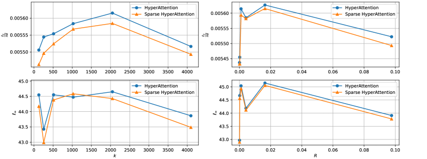
Figure 1: Comparsion between HyperAttention and Sparse HyperAttention on Gaussian distributed data with different $k$ or $R$.

In this experiment, we simple the weight of attention $W_{Q},W_{K}\in\mathbb{R}^{d\times d}$ for ${\sf d=64}$ from Gaussian distribution $\mathcal{N}(0,b)$ where $b$ is chosen from $\{0.0001,0.0002,0.0005,0.001,0.002,0.005\}$ to control the value of $R$ (Definition 4.2). And the Value projection matrix $W_{V}\in\mathbb{R}^{d\times d}$ is generate from $\mathcal{N}(0,1)$. We evaluate the $\ell_{2}$ and $\ell_{\infty}$ error of HyperAttention and Sparse HyperAttention within ${\sf T=10000}$ times, for each time we sample $X\in\mathbb{R}^{n\times d}$ where ${\sf n=2^{15}=32768}$ from Gaussian distribution $\mathcal{N}(0,1)$. Moreover, we choose the sparsity $k$ as the block size of our algorithm from $\{128,256,512,1024,2048,4096\}$. When we compare different $k$, $R$ is set to $0.4$ and when we compare different $R$, $k$ is set to $256$. The results in Figure 1 indicate that our method can demonstrate less error of approximated attention, which leads the improvement of our method in comparison with HyperAttention and they also verify the correctness of our theory.

6.2 Performance on LongBench

In this experiment, we follow the methodology of evaluation in [38]. By applying fast attention algorithms to the pre-trained LLMs chatglm2-6b-32k [87, 28], we appraise the accuracy of our method on the LongBench-E benchmark [6], which is a dataset focusing on measuring the long context ability of LLMs. Due to the more significant performance degradation of LLMs in long contexts, we only demonstrated and compared the performance of the models when the data context length exceeds $8k$. As illustrated in Table 1, our method maintains a high level of performance. When compared to HyperAttention, our method exhibits substantial robustness, especially when applied across multiple layers. This suggests that our method is not only competitive but might also offer improved performance when dealing with longer context lengths.

Algorithm with Number of Replaced Layers	Task						Average
	single-qa	multi-qa	summarization	few-shot	synthetic	code
0 (exact)∗	80.63	68.14	53.12	186.58	84.00	99.57	95.34
HyperAttention-7∗	72.34	65.37	52.54	182.12	82.00	102.06	92.74
HyperAttention-14∗	71.32	62.97	52.13	169.02	80.00	92.12	87.93
HyperAttention-21∗	44.75	48.91	50.90	150.44	31.00	82.58	68.10
HyperAttention-28∗	27.07	22.65	46.28	65.74	8.33	73.68	40.63
Sparse HyperAttention-7	60.80	60.85	52.61	184.63	50.00	98.83	84.62
Sparse HyperAttention-14	60.02	55.84	52.13	180.04	46.00	97.22	81.88
Sparse HyperAttention-21	55.31	47.46	51.79	169.81	40.11	96.09	76.76
Sparse HyperAttention-28	45.06	45.95	50.02	128.45	30.08	85.88	64.24

Table 1: Performance evaluation of chatglm2-6b-32k equipped with HyperAttentions and Sparse HyperAttention on LongBench-E datasets [6]. They contain 6 different tasks and we evaluate each of them with its own metric where higher value indicates better performance. ^∗ denotes the results is from [38].

7 Conclusion

Prior fast algorithms for enhancing the efficiency of language models alleviate the quadratic time complexity of attention computation by assuming attention sparsity, whereas these algorithms lack sufficient understanding of it. This work provides the first theoretical analysis of attention sparsity, furthermore, our theory leads to an obvious but important conclusion, that is Attention is Naturally Sparse with Gaussian Distributed Input. In addition, sparsity theory has brought us unexpected insights, one of which is the positive correlation between sparsity and attention weight norm R, directly solving the problem of prioritizing the application of fast algorithms in language models. Finally, the error analysis of sparse attention computation benefits from our theory, in which we simplified HyperAttention by introducing a scaled coefficient since the $(\epsilon,k)$-sparsity could be estimated, leads a clearer upper bound on error.

Appendix

Roadmap.

We organize the appendix as followed. In Section A, we provide more works that are related to this paper. In Section B we give some more preliminaries. In Section C we show that $KQ_{i}^{\top}$ is Gaussian distributed. In Section D we show sparsity of attention with upper bound. In Section E we provide analysis of our proposed algorithm.

Appendix A More Related Work

To complete the background of the related research, we provide some more related work in this section. The attention mechanism’s computational intensity, particularly within transformer architectures, has been a significant focus, with [29] delving into the theoretical aspects of data recovery via attention weights. Concurrently, the analysis of softmax attention’s superiority by [30] and the innovative attention schemes inspired by softmax regression from [25] contribute vital insights into attention mechanism optimization. The discourse extends to the computational frameworks of LLMs, where the theoretical examination of modern Hopfield models by [39] and the exploration of sparse Hopfield models by [42] align closely with our research’s objectives. Moreover, the innovative STanHop model by [79] and the outlier-efficient Hopfield layers presented by [36] further underscore the burgeoning interest in enhancing computational efficiencies within neural architectures. In parallel, studies on various algorithmic optimizations, such as randomized and deterministic attention sparsification [27], dynamic kernel sparsifiers [22], and zero-th order algorithms for softmax attention optimization [24], provide a comprehensive backdrop to our investigation into attention score sparsity. Further extending the discourse, studies by [80], [37], and Wu et al. [78] delve into novel applications and optimizations of Hopfield networks, showcasing the diverse avenues for computational enhancement in neural network models. [19, 18] offer additional perspectives on optimizing LLMs, addressing copyright data protection and fine-tuning for unbiased in-context learning, which underscore the multifaceted challenges in LLM research. The work by [73] on learning rate schedules further informs our understanding of model optimization and training efficiency. Moreover, the diverse array of research spanning from Fourier circuits in neural networks [31], domain generalization [66], multitask finetuning [82], to semi-supervised learning frameworks [68, 71] and spectral analysis in class discovery [69] offers a rich backdrop against which our work is situated. The Attention Sink phenomenon, discovered by [81, 8] and is helping to enhance LLMs in [83, 52], is a distinct characteristic commonly observed in most attention networks of LLMs. This phenomenon is characterized by the disproportionate attention these models pay to a specific, often unrelated, token—usually the first token. These tokens are assigned high attention scores, indicating their significant influence within the network. These studies, along with [65, 23, 70, 67] and [61, 57, 56, 32, 60, 58, 59] contributions in algorithmic optimizations and neural network analysis, not only broaden the landscape of our research but also underscore the dynamic and multifaceted nature of computational efficiency and theoretical analysis in the field of LLMs and beyond.

Appendix B Preliminary

In Section B.1 we provide some notations. In Section B.2 we provide definitions related to attention computation. In Section B.3 we provide definitions of inputs. In Section B.4 we provide the problem definition. In Section B.5 we provide some useful definitions. In Section B.6 we show some related facts about random variables. In Section B.7 we provide some fact for softmax computation.

B.1 Notations

In this work, we use the following notations and definitions: For integer $n$, we use $[n]$ to denote the set $\{1,\dots,n\}$. We use $\mathbf{1}_{n}$ to denote all-$1$ vector in $\mathbb{R}^{n}$. The $\ell_{p}$ norm of a vector $x$ is denoted as $\|x\|_{p}$, for examples, $\|x\|_{1}:=\sum^{n}_{i=1}|x_{i}|$, $\|x\|_{2}:=(\sum^{n}_{i=1}x_{i}^{2})^{1/2}$ and $\|x\|_{\infty}:=\max_{i\in[n]}|x_{i}|$. For a vector $x\in\mathbb{R}^{n}$, $\exp(x)\in\mathbb{R}^{n}$ denotes a vector where whose i-th entry is $\exp(x_{i})$ for all $i\in[n]$. For two vectors $x,y\in\mathbb{R}^{n}$, we denote $\langle x,y\rangle=\sum^{n}_{i=1}$ for $i\in[n]$. Given two vectors $x,y\in\mathbb{R}^{n}$, we denote $x\circ y$ as a vector whose i-th entry is $x_{i}y_{i}$ for all $i\in[n]$. Let $x\in\mathbb{R}^{n}$ be a vector. For a vector $x\in\mathbb{R}^{n}$, $\operatorname{diag}(x)\in\mathbb{R}^{n\times n}$ is defined as a diagonal matrix with its diagonal entries given by $\operatorname{diag}(x)_{i,i}=x_{i}$ for $i=1,...,n$, and all off-diagonal entries are $0$. We use $\operatorname*{{\mathbb{E}}}[x]$ to denote the expectation value of random variable $x\in\mathbb{R}^{n}$. We use $\operatorname*{\mathrm{Var}}[x]$ to denote the variance value of random variable $x\in\mathbb{R}^{n}$. We use $\mathrm{erf}(x)$ to denote the error function $\mathrm{erf}(x)=\frac{2}{\sqrt{\pi}}\int_{0}^{x}\exp(-t^{2})\mathrm{d}t$, and $\mathrm{erf}^{-1}$ is denoted as the inverse function of $\mathrm{erf}(x)$. For any matrix $A\in\mathbb{R}^{m\times n}$, we use $A^{\top}$ to denote its transpose, we use $\|A\|_{F}$ to denote the Frobenius norm and $\|A\|_{\infty}$ to denote its infinity norm, i.e., $\|A\|_{F}:=(\sum_{i\in[m]}\sum_{j\in[n]}A_{i,j}^{2})^{1/2}$ and $\|A\|_{\infty}=\max_{i\in[m],j\in[n]}|A_{i,j}|$. For $\mu,\sigma\in\mathbb{R}$, we use $\mathcal{N}(\mu,\sigma^{2})$ to denote Gaussian distribution with expectation of $\mu$ and variance of $\sigma^{2}$. For a mean vector $\mu\in\mathbb{R}^{d}$ and a covariance matrix $\Sigma\in\mathbb{R}^{d\times d}$, we use $\mathcal{N}(\mu,\Sigma^{2})$ to denote the vector Gaussian distribution. We use $\operatorname*{{\mathbb{E}}}[\cdot]$ to denote the expectation and $\operatorname*{\mathrm{Var}}[\cdot]$ to denote the variance.

B.2 Attention Computation with Layer Normalization

Here we introduce the following definitions about attention with layer normalization.

Definition B.1 (Layer normalization).

Given an input matrix $X\in\mathbb{R}^{n\times d}$, and given weight and bias parameters $\gamma,\beta\in\mathbb{R}^{d}$. We define the layer normalization $Ln(X)$ and the $i$-th row of $Ln(X)$ for $i\in[n]$ satisfies

$$Ln(X)_{i}=\frac{X_{i}-\operatorname*{{\mathbb{E}}}[X_{i}]\cdot{\bf 1}_{d}}{\sqrt{\operatorname*{\mathrm{Var}}[X_{i}]}}\circ\gamma+\beta$$

where $\operatorname*{{\mathbb{E}}}[X_{i}]=\frac{1}{d}\sum_{j=1}^{d}X_{i,j}$ denotes the mean value of entries of $X_{i}$ and $\operatorname*{\mathrm{Var}}[X_{i}]=\frac{1}{d}\sum_{j=1}^{d}(X_{i,j}-\operatorname*{{\mathbb{E}}}[X_{i}])$ denotes the variance of entries of $X_{i}$.

Definition B.2 (Attention computation).

Given Query, Key and Value projection matrices of attention $W_{Q},W_{K},W_{V}\in\mathbb{R}^{d\times d}$, given an input matrix $X\in\mathbb{R}^{n\times d}$ as the output of layer normalization in Definition B.1. We denote the Query, Key and Value states matrices as $Q\in\mathbb{R}^{n\times d}:=XW_{Q}$, $K\in\mathbb{R}^{n\times d}:=XW_{K}$, $V\in\mathbb{R}^{n\times d}:=XW_{V}$, then we have attention computation as follows:

$${\sf Attn}(Q,K,V):=D^{-1}AV$$

where $A\in\mathbb{R}^{n\times n}:=\exp(QK^{\top})$ and $D=\operatorname{diag}(A{\bf 1}_{n})$.

B.3 Gaussian Distributed Inputs

We define the following Gaussian distributed property of inputs.

Definition B.3.

We denote the original input matrix as $I\in\mathbb{R}^{n\times d}$, then we define $X\in\mathbb{R}^{n\times d}$ is normalized $I$ such that for $i\in[n]$, $X_{i}:=\frac{I_{i}-\operatorname*{{\mathbb{E}}}[I_{i}]\cdot{\bf 1}_{d}}{\sqrt{\operatorname*{\mathrm{Var}}[I_{i}]}}$, thus we say $X$ is Gaussian distributed, which is for $i\in[n]$ and $j\in[d]$,

$$X_{i,j}\sim\mathcal{N}(0,1).$$

Meanwhile, for $i\in[n]$, we have

$$Ln(I)_{i}=X_{i}\circ\gamma+\beta$$

B.4 Problem Definition: $\epsilon$-Approximated $k$-Sparse Softmax

In order to describe the sparsity of the softmax, we define the following notation.

Definition B.4 ($(\epsilon,k)$-sparsity ).

For a vector $u\in\mathbb{R}^{n}$, if for a constant $\epsilon\in(0,1)$, it holds that

$$|\{i\in[n]~{}|~{}|u_{i}|\leq\epsilon\}|\geq n-k,$$

then we say vector $u$ is $(\epsilon,k)$-sparse.

Definition B.5.

Suppose given error parameters $\epsilon\in(0,1)$ and a sparsity integer $k\in[0,n]$. Let $D\in\mathbb{R}^{n\times n}$ and $A\in\mathbb{R}^{n\times n}$ be defined as Definition B.2. For any $i\in[n]$, we denote the probability of vector $D_{i,i}^{-1}A_{i}$ is $(\epsilon,k)$-sparse as $P_{\it sparse}(\epsilon,k)$.

B.5 Helpful Definitions

We introduce the following algebraic lemmas to be used later.

Definition B.6.

Let $\beta\in\mathbb{R}^{d}$ be defined as Definition B.1. We define $B\in\mathbb{R}^{n\times d}$ where for $i\in[n]$, its $i$-th row satisfies

$$B_{i}=\beta^{\top}$$

Definition B.7.

Let Query and Key projection matrices $W_{Q},W_{K}\in\mathbb{R}^{d\times d}$ be defined as Definition B.2. We define

$$W:=W_{Q}W_{K}^{\top}/\sqrt{d}$$

B.6 Basic Facts for Random Variable

We introduce some basic facts for the random variables.

Fact B.8.

We have the following basic facts for random variables:

• Vector $u\in\mathbb{R}^{d}\sim\mathcal{N}(0,1)$, for any vector $v\in\mathbb{R}^{d}$, $\langle u,v\rangle\sim\mathcal{N}(0,\operatorname*{{\mathbb{E}}}[\|v\|_{2}^{2}])$.

• Matrix $U\in\mathbb{R}^{d_{1}\times d_{2}}$, for vector $v\in\mathbb{R}^{d_{2}}\sim\mathcal{N}(0,1)$, $i\in[d_{1}]$, $U_{i}v\sim\mathcal{N}(0,\operatorname*{{\mathbb{E}}}[\|U_{i}\|_{2}^{2}])$.

• Matrix $U\in\mathbb{R}^{d_{1}\times d_{2}}$, for vector $v\in\mathbb{R}^{d_{2}}\sim\mathcal{N}(0,1)$, $i\in[d_{1}]$, $\operatorname*{{\mathbb{E}}}[\|Uv\|_{2}^{2}]=\operatorname*{{\mathbb{E}}}[\|U\|_{F}^{2}]$

• Matrix $U\in\mathbb{R}^{d_{1}\times d_{2}}\sim\mathcal{N}(0,1)$, for any vector $v\in\mathbb{R}^{d_{2}}$, $U_{i}v\sim\mathcal{N}(0,\operatorname*{{\mathbb{E}}}[\|v\|_{2}^{2}])$.

• Vector $u\in\mathbb{R}^{d}\sim\mathcal{N}(0,a)$ and vector $v\in\mathbb{R}^{d}\sim\mathcal{N}(0,b)$ for $a,b>0$, then $u+v\sim\mathcal{N}(0,a+b)$.

Fact B.9.

We have the following basic facts for probability functions of random variables:

• For a random variable $x\sim\mathcal{N}(\mu,\sigma^{2})$ where $\mu,\sigma\in\mathbb{R}$, for any constant $a\in\mathbb{R}$, the probability of $x=y$ is $\Pr[x=a]=\frac{1}{\sigma\sqrt{2\pi}}\exp(-\frac{(a-\mu)^{2}}{2\sigma^{2}})$.

• For a random variable $x\sim\mathcal{N}(\mu,\sigma^{2})$ where $\mu,\sigma\in\mathbb{R}$, for any $a,b\in\mathbb{R}$, the probability of $x=y$ is

  $$\Pr[a<x<b]= ~{}\int_{a}^{b}\frac{1}{\sigma\sqrt{2\pi}}\exp(-\frac{(a-\mu)^{2}}{2\sigma^{2}})\mathrm{d}x$$

  $$= ~{}\frac{1}{2}({\rm erf}(\frac{b-\mu}{\sigma\sqrt{2}})-{\rm erf}(\frac{a-\mu}{\sigma\sqrt{2}}))$$

  .

B.7 Basic Fact for Softmax Computation

We have the following basic observation of softmax.

Fact B.10.

Given an input $x\in\mathbb{R}^{d}$, we define softmax computation as follows:

$${\sf softmax}(x):=\langle\exp(x),{\bf 1}_{n}\rangle^{-1}\exp(x).$$

For any constant $a\in\mathbb{R}$, we have

$${\sf softmax}(x)={\sf softmax}(x+a\cdot{\bf 1}_{d})$$

Appendix C $KQ_{i}^{\top}$ is Gaussian Distributed

In Section C.1 we state our main result. In Section C.2 we show how to split $KQ_{i}^{\top}$ into for terms. And in Sections C.3, C.4, C.5, we show the properties for the terms $U_{1},U_{2},U_{3}$ to be Gaussian distributed respectively.

C.1 Main Result

Here we provide the following lemma, telling that $KQ_{i}^{\top}$ is Gaussian distributed with Gaussian distributed inputs.

Lemma C.1.

If the following conditions are held:

• Let Query and Key state matrices $Q,K\in\mathbb{R}^{n\times d}$ be defined as Definition B.2.

• Let $W\in\mathbb{R}^{d}$ be defined as Definition B.7.

• Let $Ln(X)$ be defined as Definition B.1.

• Let $\gamma\in\mathbb{R}^{d}$ be defined as Definition B.1.

• Let $I,X\in\mathbb{R}^{n\times d}$ be defined as Definition B.3.

• Let $B\in\mathbb{R}^{n\times d}$ be defined as Definition B.6.

• Denote $U_{1}:=X\operatorname{diag}(\gamma)W\operatorname{diag}(\gamma)^{\top}X_{i}^{\top}$.

• Denote $U_{2}:=X\operatorname{diag}(\gamma)WB_{i}^{\top}$.

• Denote $U_{3}:=BW\operatorname{diag}(\gamma)^{\top}X_{i}^{\top}$.

• Denote $R_{1}:=\|\operatorname{diag}(\gamma)W\operatorname{diag}(\gamma)^{\top}\|_{F}^{2}$.

• Denote $R_{2}:=\|\operatorname{diag}(\gamma)W\beta\|_{2}^{2}$.

• Denote $R_{3}:=\|\beta^{\top}W\operatorname{diag}(\gamma)^{\top}\|_{2}^{2}$.

• Denote $R:=R_{1}+R_{2}+R_{3}$.

• Denote $b:=\beta^{\top}W\beta$.

Then for any $i\in[n]$, we have

$$KQ_{i}\sim\mathcal{N}(b,R)$$

Proof.

We have

$$KQ_{i}= ~{}U_{1}+U_{2}+U_{3}+b\cdot{\bf 1}_{d}$$

$$\sim ~{}\mathcal{N}(b,R_{1}+R_{2}+R_{3})$$

$$\sim ~{}\mathcal{N}(b,R)$$

where the first step follows from Lemma C.2, the second step follows from Lemma C.3, Lemma C.4 and Lemma C.5, the last step follows from $R=R_{1}+R_{2}+R_{3}$. ∎

C.2 Split $KQ_{i}^{\top}$

We introduce the following lemma to split the term $KQ_{i}^{\top}$.

Lemma C.2.

If the following conditions are held:

• Let Query and Key state matrices $Q,K\in\mathbb{R}^{n\times d}$ be defined as Definition B.2.

• Let $W\in\mathbb{R}^{d}$ be defined as Definition B.7.

• Let $Ln(X)$ be defined as Definition B.1.

• Let $\gamma\in\mathbb{R}^{d}$ be defined as Definition B.1.

• Let $I,X\in\mathbb{R}^{n\times d}$ be defined as Definition B.3.

• Let $B\in\mathbb{R}^{n\times d}$ be defined as Definition B.6.

• Denote $U_{1}:=X\operatorname{diag}(\gamma)W\operatorname{diag}(\gamma)^{\top}X_{i}^{\top}$.

• Denote $U_{2}:=X\operatorname{diag}(\gamma)WB_{i}^{\top}$.

• Denote $U_{3}:=BW\operatorname{diag}(\gamma)^{\top}X_{i}^{\top}$.

• Denote $b:=\beta^{\top}W\beta$.

We have

$$KQ_{i}^{\top}= ~{}(X\operatorname{diag}(\gamma)+B)W(X_{i}\operatorname{diag}(\gamma)+B_{i})^{\top}$$

$$= ~{}U_{1}+U_{2}+U_{3}+b\cdot{\bf 1}_{d}$$

Proof.

We have

$$KQ_{i}^{\top}= ~{}Ln(I)WLn(I)_{i}$$

$$= ~{}(X\operatorname{diag}(\gamma)+B)W(X_{i}\operatorname{diag}(\gamma)+B_{i})^{\top}$$

$$= ~{}X\operatorname{diag}(\gamma)W\operatorname{diag}(\gamma)^{\top}X_{i}^{\top}+X\operatorname{diag}(\gamma)WB_{i}^{\top}$$

$$~{}+BW\operatorname{diag}(\gamma)^{\top}X_{i}^{\top}+BWB_{i}^{\top}$$

$$= ~{}U_{1}+U_{2}+U_{3}+BWB_{i}^{\top}$$

$$= ~{}U_{1}+U_{2}+U_{3}+b\cdot{\bf 1}_{d}$$

where the first and second steps follow from Definition B.3, Definition B.6 and Definition B.7, the third step follows from simple algebra, the fourth step follows from the definitions of $U_{1}$, $U_{2}$ and $U_{3}$, the last step follows from $B_{j}=B_{k}=\beta^{\top}$ for any $j,k\in[n]$. ∎

C.3 Property for $U_{1}$ is Gaussian Distributed

Here we provide analysis for the first term $U_{1}$.

Lemma C.3.

If the following conditions are held:

• Let Query and Key state matrices $Q,K\in\mathbb{R}^{n\times d}$ be defined as Definition B.2.

• Let $W\in\mathbb{R}^{d}$ be defined as Definition B.7.

• Let $I,X\in\mathbb{R}^{n\times d}$ be defined as Definition B.3.

• Denote $U_{1}:=X\operatorname{diag}(\gamma)W\operatorname{diag}(\gamma)^{\top}X_{i}^{\top}$ as Lemma C.2.

• Denote $R_{1}:=\|\operatorname{diag}(\gamma)W\operatorname{diag}(\gamma)^{\top}\|_{F}^{2}$.

We have

$$U_{1}\sim\mathcal{N}(0,R_{1})$$

Proof.

For $j\in[n]$, we have

$$\operatorname{diag}(\gamma)_{j,j}W_{j}\operatorname{diag}(\gamma)^{\top}X_{i}^{\top}\sim\mathcal{N}(0,\|\operatorname{diag}(\gamma)W\operatorname{diag}(\gamma)^{\top}\|_{F}^{2})$$ (1)

where this step follows from Fact B.8.

Then, we can get

$$~{}U_{1}$$

$$= ~{}X\operatorname{diag}(\gamma)W\operatorname{diag}(\gamma)^{\top}X_{i}^{\top}$$

$$\sim ~{}\mathcal{N}(0,\operatorname*{{\mathbb{E}}}[\|\operatorname{diag}(\gamma)_{j,j}W_{j}\operatorname{diag}(\gamma)^{\top}X_{i}^{\top}\|_{2}^{2}])$$

$$\sim ~{}\mathcal{N}(0,\operatorname*{{\mathbb{E}}}[\|\operatorname{diag}(\gamma)_{j,j}W_{j}\operatorname{diag}(\gamma)^{\top}X_{i}^{\top}\|_{2}^{2}]-\sum_{j=1}^{d}\operatorname*{{\mathbb{E}}}[\operatorname{diag}(\gamma)_{j,j}W_{j}\operatorname{diag}(\gamma)^{\top}X_{i}^{\top}]^{2})$$

$$\sim ~{}\mathcal{N}(0,\sum_{j=1}^{d}\operatorname*{\mathrm{Var}}[\operatorname{diag}(\gamma)_{j,j}W_{j}\operatorname{diag}(\gamma)^{\top}X_{i}^{\top}])$$

$$\sim ~{}\mathcal{N}(0,\|\operatorname{diag}(\gamma)W\operatorname{diag}(\gamma)^{\top}\|_{F}^{2})$$

$$\sim ~{}\mathcal{N}(0,R_{1})$$

where the first step follows from the definition of $U_{1}$, the second step follows from Fact B.8, the third step follows from Eq. (1), the fourth step follows from $\operatorname*{\mathrm{Var}}[x]=\operatorname*{{\mathbb{E}}}[x^{2}]-\operatorname*{{\mathbb{E}}}[x]^{2}$, the fifth step follows from simple algebra and rule of matrix norm, the last step follows from the definition of $R_{1}$. ∎

C.4 Property for $U_{2}$ is Gaussian Distributed

Here we provide analysis for the second term $U_{2}$.

Lemma C.4.

If the following conditions are held:

• Let Query and Key state matrices $Q,K\in\mathbb{R}^{n\times d}$ be defined as Definition B.2.

• Let $W\in\mathbb{R}^{d}$ be defined as Definition B.7.

• Let $I,X\in\mathbb{R}^{n\times d}$ be defined as Definition B.3.

• Denote $U_{2}:=X\operatorname{diag}(\gamma)WB_{i}^{\top}$ as Lemma C.2.

• Denote $R_{2}:=\|\operatorname{diag}(\gamma)W\beta\|_{2}^{2}$.

We have

$$U_{2}\sim\mathcal{N}(0,R_{2})$$

Proof.

For $j\in[n]$, we have

$${U_{2}}_{j}= ~{}X_{j}\operatorname{diag}(\gamma)WB_{i}^{\top}$$

$$\sim ~{}\mathcal{N}(0,\|\operatorname{diag}(\gamma)WB_{i}^{\top}\|_{2}^{2})$$

$$\sim ~{}\mathcal{N}(0,\|\operatorname{diag}(\gamma)W\beta\|_{2}^{2})$$

$$\sim ~{}\mathcal{N}(0,R_{2})$$

where the first step follows from the definition of $U_{2}$, the second step follows from Fact B.8, the third step follows from $B_{i}^{\top}=\beta$ for $i\in[n]$, the last step follows from the definition of $R_{2}$. ∎

C.5 Property for $U_{3}$ is Gaussian Distributed

Here we provide analysis for the third term $U_{3}$.

Lemma C.5.

If the following conditions are held:

• Let Query and Key state matrices $Q,K\in\mathbb{R}^{n\times d}$ be defined as Definition B.2.

• Let $W\in\mathbb{R}^{d}$ be defined as Definition B.7.

• Let $I,X\in\mathbb{R}^{n\times d}$ be defined as Definition B.3.

• Denote $U_{3}:=BW\operatorname{diag}(\gamma)^{\top}X_{i}^{\top}$ as Lemma C.2.

• Denote $R_{3}:=\|\beta^{\top}W\operatorname{diag}(\gamma)^{\top}\|_{2}^{2}$.

We have

$$U_{3}\sim\mathcal{N}(0,R_{3})$$

Proof.

For $j\in[n]$, we have

$${U_{3}}_{j}= ~{}B_{j}W\operatorname{diag}(\gamma)^{\top}X_{i}^{\top}$$

$$\sim ~{}\mathcal{N}(0,\|B_{j}W\operatorname{diag}(\gamma)^{\top}\|_{2}^{2})$$

$$\sim ~{}\mathcal{N}(0,\|\beta^{\top}W\operatorname{diag}(\gamma)^{\top}\|_{2}^{2})$$

$$\sim ~{}\mathcal{N}(0,R_{3})$$

where the first step follows from the definition of $U_{3}$, the second step follows from Fact B.8, the third step follows from $B_{j}=\beta$, the last step follows from the definition of $R_{2}$. ∎

Appendix D Sparse Attention with Upper Bound of Error

In Section D.1 we show the main result. In Section D.2 we show $\operatorname*{{\mathbb{E}}}[KQ_{i}^{\top}]$ is unrelated to the softmax computation. In Section D.3 we show the upper and lower bound of $\exp(U)$. In Section D.4 we lower bound $P_{sparse}(\epsilon,k)$. In Section D.5 we provide a helpful lemma.

D.1 Main Result

We state our main theorem here, telling that the probability of vector $D_{i,i}A$ being sparse is high.

Theorem D.1 ( ).

Suppose given an integer $k\in(0,n/2]$, let the probability of vector $D_{i,i}A_{i}$ for $i\in[n]$ is $(\epsilon,k)$-sparse be defined as Definition B.5. Let constant $R>0$ be defined as Definition D.2. Then we have

$$P_{\it sparse}(\epsilon,k)\geq 0.9999,$$

with error $\epsilon\in[\epsilon_{b},1)$ where

$$\epsilon_{b}=\exp\left(\sqrt{2R}\big{(}{\rm erf}^{-1}(\frac{k-2}{k})-{\rm erf}^{-1}(2(\frac{3.9996}{\binom{n}{k}})^{\frac{1}{n-k}}-1)\big{)}\right)^{-1}$$

Proof.

Let $p(\epsilon^{-1}x)=\frac{k-1}{k}$ and $p(x)\geq(3.9996/\binom{n}{k})^{\frac{1}{n-k}}$, then we have

$$P_{\it sparse}(\epsilon,k)\geq ~{}\binom{n}{k}k(1-p(\epsilon^{-1}x))\cdot p^{k-1}(\epsilon^{-1}x)\cdot p^{n-k}(x)$$

$$= ~{}\binom{n}{k}k(\frac{1}{k})\cdot(\frac{k-1}{k})^{k-1}\cdot p^{n-k}(x)$$

$$= ~{}\binom{n}{k}(\frac{k-1}{k})^{k-1}\cdot p^{n-k}(x)$$

$$\geq ~{}0.25\binom{n}{k}\cdot p^{n-k}(x)$$

$$\geq ~{}0.25\binom{n}{k}\cdot((3.9996/\binom{n}{k})^{\frac{1}{n-k}})^{n-k}$$

$$= ~{}0.9999$$

where the first step follows from Lemma D.8, the second step follows from $p(\epsilon^{-1}x)=\frac{k-1}{k}$, the third step follows from simple algebra, the fourth step follows from Lemma D.9, the fifth step follows from $p(x)=(3.9996/\binom{n}{k})^{\frac{1}{n-k}}$, the last step follows from simple algebra.

In Eq. (D.1) we will show

$$\frac{1}{2}(\mathrm{erf}(\frac{\ln(\epsilon^{-1}x)}{R\sqrt{2}})+1) ~{}=\frac{k-1}{k}$$

is equivalent to

$$\ln(\epsilon^{-1})+\ln(x) ~{}=\sqrt{2R}\mathrm{erf}^{-1}(\frac{k-2}{k})$$

For simplicity, we use $\iff$ to denote equivalent.

When $p(\epsilon^{-1}x)=\frac{k-1}{k}$, we show

$$~{}\frac{1}{2}(\mathrm{erf}(\frac{\ln(\epsilon^{-1}x)}{\sqrt{2R}})+1)=\frac{k-1}{k}$$

$$\iff ~{}\mathrm{erf}(\frac{\ln(\epsilon^{-1}x)}{\sqrt{2R}})+1=\frac{2k-2}{k}$$

$$\iff ~{}\mathrm{erf}(\frac{\ln(\epsilon^{-1}x)}{\sqrt{2R}})=\frac{k-2}{k}$$

$$\iff ~{}\frac{\ln(\epsilon^{-1}x)}{\sqrt{2R}}=\mathrm{erf}^{-1}(\frac{k-2}{k})$$

$$\iff ~{}\ln(\epsilon^{-1}x)=\sqrt{2R}\mathrm{erf}^{-1}(\frac{k-2}{k})$$

$$\iff ~{}\ln(\epsilon^{-1})+\ln(x)=\sqrt{2R}\mathrm{erf}^{-1}(\frac{k-2}{k})$$ (2)

where the first step follows from Definition D.6, the second and third steps follow from simple algebras, the fourth step follows from applying inverse error function, the last two steps follow from simple algebras.

On the other hand, when $p(x)\geq(3.9996/\binom{n}{k})^{\frac{1}{n-k}}$, we have

$$~{}\frac{1}{2}(\mathrm{erf}(\frac{\ln(x)}{\sqrt{2R}})+1)\geq(3.9996/\binom{n}{k})^{\frac{1}{n-k}}$$

$$\iff ~{}\mathrm{erf}(\frac{\ln(x)}{\sqrt{2R}})\geq 2(3.9996/\binom{n}{k})^{\frac{1}{n-k}}-1$$

$$\iff ~{}\frac{\ln(x)}{\sqrt{2R}}\geq\mathrm{erf}^{-1}(2(3.9996/\binom{n}{k})^{\frac{1}{n-k}}-1)$$

$$\iff ~{}\ln(x)\geq\sqrt{2R}\mathrm{erf}^{-1}(2(3.9996/\binom{n}{k})^{\frac{1}{n-k}}-1)$$ (3)

where the first step follows from Definition D.6, the second step follows from simple algebras, the third step follows from applying inverse error function, the last step follows from simple algebras.

Combining Eq. D.1 and Eq. (D.1), we have

$$~{}\ln(\epsilon^{-1})\geq\sqrt{2}R\mathrm{erf}^{-1}(\frac{k-2}{k})-\sqrt{2R}\mathrm{erf}^{-1}(2(3.9996/\binom{n}{k})^{\frac{1}{n-k}}-1)$$

$$\iff ~{}\epsilon^{-1}\geq\exp(\sqrt{2R}\mathrm{erf}^{-1}(\frac{k-2}{k})-\sqrt{2R}\mathrm{erf}^{-1}(2(3.9996/\binom{n}{k})^{\frac{1}{n-k}}-1))$$

$$\iff ~{}\epsilon\geq\exp(\sqrt{2R}\mathrm{erf}^{-1}(\frac{k-2}{k})-\sqrt{2R}\mathrm{erf}^{-1}(2(3.9996/\binom{n}{k})^{\frac{1}{n-k}}-1))^{-1}$$

$$\iff ~{}\epsilon\geq\exp\left(\sqrt{2R}\big{(}{\rm erf}^{-1}(\frac{k-2}{k})-{\rm erf}^{-1}(2(\frac{3.9996}{\binom{n}{k}})^{\frac{1}{n-k}}-1)\big{)}\right)^{-1}$$

where the first step follows from Eq. (D.1) and Eq. (D.1), the second, third and fourth steps follow from simple algebras. ∎

D.2 $\operatorname*{{\mathbb{E}}}[KQ_{i}^{\top}]$ is Unrelated to the Softmax Computation

We first state the following two definitions.

Definition D.2.

If the following conditions are held:

• Let Query and Key state matrices $Q,K\in\mathbb{R}^{n\times d}$ be defined as Definition B.2.

• Let $W\in\mathbb{R}^{d}$ be defined as Definition B.7.

• Let $\gamma,\beta\in\mathbb{R}^{d}$ be defined as Definition B.1.

• Let $X\in\mathbb{R}^{n\times d}$ be defined as Definition B.3.

We define

$$R=\|\operatorname{diag}(\gamma)W\operatorname{diag}(\gamma)^{\top}\|_{F}^{2}+\|\operatorname{diag}(\gamma)W\beta\|_{2}^{2}+\|\beta^{\top}W\operatorname{diag}(\gamma)^{\top}\|_{2}^{2}$$

Definition D.3.

If the following conditions are held:

• Let Query and Key state matrices $Q,K\in\mathbb{R}^{n\times d}$ be defined as Definition B.2.

• Let $W\in\mathbb{R}^{d}$ be defined as Definition B.7.

• Let $\gamma\in\mathbb{R}^{d}$ be defined as Definition B.1.

• Let $X\in\mathbb{R}^{n\times d}$ be defined as Definition B.3.

• Let $B\in\mathbb{R}^{n\times d}$ be defined as Definition B.6.

• Denote $U_{1}:=X\operatorname{diag}(\gamma)W\operatorname{diag}(\gamma)^{\top}X_{i}^{\top}$ as Lemma C.2.

• Denote $U_{2}:=X\operatorname{diag}(\gamma)WB_{i}^{\top}$ as Lemma C.2.

• Denote $U_{3}:=BW\operatorname{diag}(\gamma)^{\top}X_{i}^{\top}$ as Lemma C.2.

• Let $R>0$ be defined as Definition D.2.

• Denote $b:=\beta^{\top}W\beta$.

We following Lemma C.2 and Lemma C.1, define

$$U= ~{}KQ_{i}^{\top}-b\cdot{\bf 1}_{n}$$

$$= ~{}U_{1}+U_{2}+U_{3}$$

$$\sim ~{}\mathcal{N}(0,R)$$

Now we are able to give the following lemma telling that $\operatorname*{{\mathbb{E}}}[KQ_{i}^{\top}]$ is independent with softmax computation.

Lemma D.4.

If the following conditions are held:

• Let Query and Key state matrices $Q,K\in\mathbb{R}^{n\times d}$ be defined as Definition B.2.

• Let $W\in\mathbb{R}^{d}$ be defined as Definition B.7.

• Let $Ln(X)$ be defined as Definition B.1.

• Let $\gamma,\beta\in\mathbb{R}^{d}$ be defined as Definition B.1.

• Let $I,X\in\mathbb{R}^{n\times d}$ be defined as Definition B.3.

• Let $B\in\mathbb{R}^{n\times d}$ be defined as Definition B.6.

• Denote $U\in\mathbb{R}^{n}$ be defined as Definition D.3

• Denote $b:=\beta^{\top}W\beta$.

We have

$$\langle\exp(KQ_{i}^{\top}),{\bf 1}_{n}\rangle^{-1}\exp(KQ_{i}^{\top})=\langle\exp(U),{\bf 1}_{n}\rangle^{-1}\exp(U)$$

Proof.

This proof is following $U=KQ_{i}^{\top}+b\cdot{\bf 1}_{n}$ and Fact B.10. ∎

D.3 Upper Bound and Lower Bound on $\exp(U)$

Here we prove the following lemmas, telling the upper and lower bound on $\exp(U)$.

Lemma D.5.

Let $U\in\mathbb{R}^{n}$ be defined as Definition D.3, for $i\in[n]$, since $U$ is following Gaussian distribution $\mathcal{N}(0,R)$ where constant $R$ is defined as Definition D.2, then denote $a,b>0$, we have

$$\Pr[a\leq\exp(U_{i})\leq b]=\frac{1}{2}(\mathrm{erf}(\frac{\ln(b)}{\sqrt{2R}})-\mathrm{erf}(\frac{\ln(a)}{\sqrt{2R}}))$$

Proof.

This proof is following Fact B.9. ∎

For convenience, we utilize $p(x)$ to denote the probability of $\exp(U_{i})<x$ for $x>0$ and for $i\in[n]$ as follows:

Definition D.6.

Let $U\in\mathbb{R}^{n}$ be defined as Definition D.3, for $i\in[n]$, since $U$ is following Gaussian distribution $\mathcal{N}(0,R)$ where constant $R$ is defined as Definition D.2, for $x>0$, we define

$$p(x)= ~{}\Pr[\exp(U_{i})\leq x]$$

$$= ~{}\frac{1}{2}({\rm erf}(\frac{\ln(x)}{\sqrt{2R}})+1)$$

Lemma D.7.

Let $U\in\mathbb{R}^{n}$ be defined as Definition D.3, for $i\in[n]$, since $U$ is following Gaussian distribution $\mathcal{N}(0,R)$ where constant $R$ is defined as Definition D.2. Let $p(x)$ be denoted as Definition D.6, we have

$$\Pr[\langle\exp(U),{\bf 1}_{n}\rangle\geq x]\geq n(1-p(x))\cdot p^{n-1}(x)$$

Proof.

We consider one case only for $\langle\exp(U),{\bf 1}_{n}\rangle\geq x$: there is only one entry $i$ in $\exp(U)$ that $\exp(U_{i})>x$ and other $\exp(U_{j})\leq x$ for $j\in[n],j\neq i$. We have

$$\Pr[\langle\exp(U),{\bf 1}_{n}\rangle\geq x]\geq ~{}\binom{n}{1}\Pr[\exp(U_{i})\leq x]^{n-1}\cdot\Pr[\exp(U_{i})>x]$$

$$= ~{}n\Pr[\exp(U_{i})\leq x]^{n-1}\cdot\Pr[\exp(U_{i})>x]$$

$$= ~{}n\Pr[\exp(U_{i})\leq x]^{n-1}\cdot(1-\Pr[\exp(U_{i})\leq x])$$

$$= ~{}n(1-p(x))\cdot p^{n-1}(x)$$

where the first step follows from simple probability rule, the second step follows from $\binom{n}{1}=n$, the third step follows from $\Pr[\exp(U_{i})\leq x]+\Pr[\exp(U_{i})>x]=1$, the last step follows from Definition D.6. ∎

D.4 Lower Bound on $P_{\it sparse}(\epsilon,k)$

Now we give the lower bound of $P_{\it sparse}(\epsilon,k)$.

Lemma D.8.

Suppose given error parameters $\epsilon\in(0,1)$ and a sparsity integer $k\in(0,n/2]$. Let $D\in\mathbb{R}^{n\times n}$ and $A\in\mathbb{R}^{n\times n}$ be defined as Definition B.2. For any $i\in[n]$, denote the probability of vector $D_{i,i}^{-1}A_{i}=\langle\exp(KQ_{i}^{\top}),{\bf 1}_{n}\rangle^{-1}\exp(KQ_{i}^{\top})$ is $(\epsilon,k)$-sparse $P_{\it sparse}(\epsilon,k)$ as Definition B.5, then we have

$$P_{\it sparse}(\epsilon,k)\geq\min\{1,\max_{x>0}\binom{n}{k}k(1-p(\epsilon^{-1}x))\cdot p^{k-1}(\epsilon^{-1}x)\cdot p^{n-k}(x)\}$$

Proof.

Firstly, following Lemma D.4, we have

$$\langle\exp(KQ_{i}^{\top}),{\bf 1}_{n}\rangle^{-1}\exp(KQ_{i}^{\top})=\langle\exp(U_{i}),{\bf 1}_{n}\rangle^{-1}\exp(U_{i})$$

Next, we can show that

$$P_{\it sparse}(\epsilon k)\geq ~{}\binom{n}{k}\Pr[\exp(U_{i})\leq x]^{n-k}\cdot\Pr[\langle\exp(U),{\bf 1}_{k}\rangle\geq\epsilon^{-1}x]$$

$$= ~{}\binom{n}{k}p^{n-k}(x)\cdot\Pr[\langle\exp(U),{\bf 1}_{k}\rangle\geq\epsilon^{-1}x]$$

$$\geq ~{}\binom{n}{k}k(1-p(\epsilon^{-1}x))\cdot p^{k-1}(\epsilon^{-1}x)\cdot p^{n-k}(x)$$

where the first step follows from simple probability rule, the second step follows from Definition D.6, the last step follows from Lemma D.7. ∎

D.5 Helpful Lemmas

We state the following fact.

Fact D.9.

For an integer $n\geq 2$, we have

$$(1-\frac{1}{n})^{n}\geq 1/4$$

Proof.

We have

$$\frac{\mathrm{d}}{\mathrm{d}x}(\frac{n-1}{n})^{n}=\frac{(\frac{n-1}{n})^{n}((x-1)\log(\frac{x-1}{x})+1)}{n-1}$$ (4)

where this step follows from simple differential rule.

When $n\geq 1$, Eq.(4) is positive, so it’s easy to have when $n$ increases, $(\frac{n-1}{n})^{n}$ increases, too.

Hence, we have

$$(\frac{n-1}{n})^{n}\geq 1/4$$

where this step follows from $n\geq 2$ and Eq.(4). ∎

Appendix E Analysis

In Section E.1 we show the main result. In Section E.2 we provide some helpful definitions. In Section E.3 we provide upper bound on difference of $DAV$ and $\widetilde{D}\widetilde{A}V$. In Section E.4 we provide upper bound on difference of $DA$ and $\widetilde{D}\widetilde{A}$. In Section E.5 we provide upper bound on difference of $D$ and $\widetilde{D}$. In Section E.6 we show the bound on $A$ over $D$. In Section E.7 we show the bound on $\widetilde{D}$ and $D$.

E.1 Main Result

We provide the following theorem, telling the approximation guarantee of Algorithm 1.

Theorem E.1 ( ).

Given Query, Key and Value states matrices $Q,K,V\in R^{n\times d}$ as Definition B.2. For a positive integer $k\in(0,n/2]$, let $\epsilon_{b}$ be denoted as Theorem D.1. Choose a integer $r>0$ as Definition 5.1. Assuming Algorithm 1 returns an approximation $T\in\mathbb{R}^{n\times d}=\widetilde{D}^{-1}\widetilde{A}V$ on attention output ${\sf Attn}(Q,K,V)$ in Definition B.2 within time complexity $O(nkd+2ndr)$, where $\widetilde{D}$ and $\widetilde{A}$ are defined in Definition E.3 and Definition E.2, and we have

$$\|T-{\sf Attn}(Q,K,V)\|_{\infty}\leq(n-k)\epsilon\cdot\|V\|_{\infty}$$

Proof.

This proof is following from Lemma E.4. ∎

E.2 Helpful Definitions

We state the following useful definitions here.

Definition E.2.

Let Query and Key state matrices $Q,K\in\mathbb{R}^{n\times d}$ be defined as Definition B.2. Also we define $A_{i}\in\mathbb{R}^{1\times n}:=\exp(Q_{i}K^{\top})$ and $D_{i,i}\in\mathbb{R}$ as Definition B.2. For $i\in[n]$, we define $\widetilde{A}_{i}\in\mathbb{R}^{1\times n}$ where for $j\in[n]$, we have

$$\widetilde{A}_{i,j}=\left\{\begin{array}[]{lr}A_{i,j},&A_{i,j}>D_{i,i}\epsilon\\ 0,&A_{i,j}\leq D_{i,i}\epsilon\end{array}\right.$$

Definition E.3.

Given sparsity integer $k\in(0,n/2]$. Let $\epsilon_{b}$ be defined as Theorem D.1. There is at most $k$ entries in vector $D^{-1}_{i,i}A_{i}\in\mathbb{R}^{1\times n}$ is bigger than $\epsilon$ where positive integer $k\in(0,n/2]$ where $D_{i,i},A_{i,j}\in\mathbb{R}$ be defined as Definition B.2 for $i,j\in[n]$. And let $\widetilde{D}_{i,i}$ be defined as Definition E.3. For $i\in[n]$, $\widetilde{A}_{i}\in\mathbb{R}^{1\times n}$ are defined as Definition E.2, we define

$$\widetilde{D}_{i,i}=\alpha\widetilde{A}_{i}{\bf 1}_{n}$$

where $\alpha:=(1-(n-k)\epsilon)^{-1}$

E.3 Upper bound on difference of $DAV$ and $\widetilde{D}\widetilde{A}V$

We prove the following lemma, giving the bound of difference between $DAV$ and $\widetilde{D}\widetilde{A}V$.

Lemma E.4.

Let Value state matrix $V\in\mathbb{R}^{n\times d}$ as Definition B.2. Given error $\epsilon\in(0,1)$. We assume that there is at most $k$ entries in vector $D^{-1}_{i,i}A_{i}\in\mathbb{R}^{1\times n}$ is bigger than $\epsilon$ where positive integer $k\in(0,n/2]$ where $D_{i,i},A_{i,j}\in\mathbb{R}$ be defined as Definition B.2 for $i,j\in[n]$. And let $\widetilde{D}_{i,i}$ be defined as Definition E.3. Let $\widetilde{A}_{i,j}\in\mathbb{R}$ be defined as Definition E.2. We have

$$\|D^{-1}AV-\widetilde{D}^{-1}\widetilde{A}V\|_{\infty}\leq(n-k)\epsilon\cdot\|V\|_{\infty}$$

Proof.

We have

$$\|D^{-1}AV-\widetilde{D}^{-1}\widetilde{A}V\|_{\infty}\leq ~{}\|D^{-1}A-\widetilde{D}^{-1}\widetilde{A}\|_{\infty}\cdot\|V\|_{\infty}$$

$$\leq ~{}\max_{i,j\in[n]}|D_{i,i}^{-1}A_{i,j}-\widetilde{D}_{i,i}^{-1}\widetilde{A}_{i,j}|\cdot\|V\|_{\infty}$$

$$\leq ~{}(n-k)\epsilon\cdot\|V\|_{\infty}$$

where the first step follows from triangle inequality, the second step follows from the definition of $\ell_{\infty}$ norm, the last step follows from Lemma E.5. ∎

E.4 Upper bound on difference of $DA$ and $\widetilde{D}\widetilde{A}$

We prove the following lemma, giving the bound of difference between $DA$ and $\widetilde{D}\widetilde{A}$.

Lemma E.5.

Given error $\epsilon\in(0,1)$.We assume that there is at most $k$ entries in vector $D^{-1}_{i,i}A_{i}\in\mathbb{R}^{1\times n}$ is bigger than $\epsilon$ where positive integer $k\in(0,n/2]$ where $D_{i,i},A_{i,j}\in\mathbb{R}$ be defined as Definition B.2 for $i,j\in[n]$. And let $\widetilde{D}_{i,i}$ be defined as Definition E.3. Let $\widetilde{A}_{i,j}\in\mathbb{R}$ be defined as Definition E.2. We have ‘

$$|D_{i,i}^{-1}A_{i,j}-\widetilde{D}_{i,i}^{-1}\widetilde{A}_{i,j}|\leq(n-k)\epsilon$$

Proof.

When $\widetilde{A}_{i,j}>0$, we have

$$|D_{i,i}^{-1}A_{i,j}-\widetilde{D}_{i,i}^{-1}\widetilde{A}_{i,j}|= ~{}|D_{i,i}^{-1}-\widetilde{D}_{i,i}^{-1}||A_{i,j}|$$

$$\leq ~{}(n-k)\epsilon(\widetilde{A}_{i}{\bf 1}_{n})^{-1}|A_{i,j}|$$

$$= ~{}(n-k)\epsilon^{1+o(1)}$$

where the first step follows from Definition E.2, the second step follows from Lemma E.6, the last step follows from Lemma E.7.

When $\widetilde{A}_{i,j}=0$, we have

$$|D_{i,i}^{-1}A_{i,j}-\widetilde{D}_{i,i}^{-1}\widetilde{A}_{i,j}|= ~{}|D_{i,i}^{-1}A_{i,j}|$$

$$\leq ~{}\epsilon$$

where these two steps follow from Definition E.2 and $\widetilde{A}_{i,j}=0$.

Combine two results, we say that

$$|D_{i,i}^{-1}A_{i,j}-\widetilde{D}_{i,i}^{-1}\widetilde{A}_{i,j}|\leq(n-k)\epsilon$$

∎

E.5 Upper bound on difference of $D$ and $\widetilde{D}$

We prove the following lemma, giving the bound of difference between $D$ and $\widetilde{D}$.

Lemma E.6.

Given error $\epsilon\in(0,1)$. We assume that there is at most $k$ entries in vector $D^{-1}_{i,i}A_{i}\in\mathbb{R}^{1\times n}$ is bigger than $\epsilon$ where positive integer $k\in(0,n/2]$ where $D_{i,i},A_{i,j}\in\mathbb{R}$ be defined as Definition B.2 for $i,j\in[n]$. And let $\widetilde{D}_{i,i}$ be defined as Definition E.3. Let $\widetilde{A}_{i,j}\in\mathbb{R}$ be defined as Definition E.2. We have

$$|D_{i,i}^{-1}-\widetilde{D}_{i,i}^{-1}|\leq(n-k)\epsilon(\widetilde{A}_{i}{\bf 1}_{n})^{-1}$$

Proof.

We have

$$|D_{i,i}^{-1}-\widetilde{D}_{i,i}^{-1}|= ~{}|\frac{1}{D_{i,i}}-\frac{1}{\widetilde{D}_{i,i}}|$$

$$= ~{}|\frac{1}{D_{i,i}}-\frac{1}{D_{i,i}-(D_{i,i}-\widetilde{D}_{i,i})}|$$

$$= ~{}|\frac{D_{i,i}-\widetilde{D}_{i,i}}{D_{i,i}^{2}-D_{i,i}(D_{i,i}-\widetilde{D}_{i,i})}|$$

$$\leq ~{}|\frac{|1-\alpha|D_{i,i}}{D_{i,i}^{2}-D_{i,i}(D_{i,i}-\widetilde{D}_{i,i})}|$$

$$= ~{}|\frac{1-\alpha}{\widetilde{D}_{i,i}}|$$

$$= ~{}|\frac{\frac{1}{\alpha}-1}{\widetilde{A}_{i}{\bf 1}_{n}}|$$

$$= ~{}(n-k)\epsilon(\widetilde{A}_{i}{\bf 1}_{n})^{-1}$$

where the first, second and third steps follow from simple algebras. The fourth step follows from Lemma E.8, the fifth step follows from simple algebra, the sixth step follows from Definition E.3, the last step follows from simple algebra and $\alpha=(1-(n-k)\epsilon)^{-1}$. ∎

E.6 Bound on $A$ over $D$

We prove the following lemma, giving the bound of $A$ over $D$.

Lemma E.7.

Given error $\epsilon\in(0,1)$. We assume that there is at most $k$ entries in vector $D^{-1}_{i,i}A_{i}\in\mathbb{R}^{1\times n}$ is bigger than $\epsilon$ where positive integer $k\in(0,n/2]$ where $D_{i,i},A_{i,j}\in\mathbb{R}$ be defined as Definition B.2 for $i,j\in[n]$. And let $\widetilde{D}_{i,i}$ be defined as Definition E.3. Let $\widetilde{A}_{i,j}\in\mathbb{R}$ be defined as Definition E.2. We have

$$\frac{\widetilde{A}_{i,j}}{\widetilde{A}_{i}{\bf 1}_{n}}\in[\epsilon,1]$$

Proof.

Since $\widetilde{A}_{i}{\bf 1}_{n}=\sum_{j=1}^{n}\widetilde{A}_{i,j}$ and $A_{i,j}>0$, we have $\frac{\widetilde{A}_{i,j}}{\widetilde{A}_{i}{\bf 1}_{n}}\leq 1$.

On the other hand, following $\widetilde{A}_{i}{\bf 1}_{n}\leq D_{i,i}$ and $A_{i,j}/D_{i,i}\geq\epsilon$, then we have $\frac{\widetilde{A}_{i,j}}{\widetilde{A}_{i}{\bf 1}_{n}}\geq\epsilon$. ∎

E.7 Bound on $\widetilde{D}$ and $D$

We prove the following lemma, giving the bound of $\widetilde{D}$ and $D$.

Lemma E.8.

Given error $\epsilon\in(0,1)$. We assume that there is at most $k$ entries in vector $D^{-1}_{i,i}A_{i}\in\mathbb{R}^{1\times n}$ is bigger than $\epsilon$ where positive integer $k\in(0,n/2]$ where $D_{i,i},A_{i,j}\in\mathbb{R}$ be defined as Definition B.2 for $i,j\in[n]$. And let $\widetilde{D}_{i,i}$ and $\alpha$ be defined as Definition E.3. Let $\widetilde{A}_{i,j}\in\mathbb{R}$ be defined as Definition E.2. We have

• Part 1.

  $$1-(n-k)\epsilon\leq\frac{\widetilde{A}_{i}{\bf 1}_{n}}{D_{i,i}}\leq 1$$

• Part 2.

  $$1\leq\frac{\widetilde{D}_{i,i}}{D_{i,i}}\leq\alpha$$

• Part 3.

  $$|D_{i,i}-\widetilde{D}_{i,j}|\leq|1-\alpha|D_{i,i}$$

Proof.

Proof of Part 1. We have

$$\frac{\widetilde{A}_{i}{\bf 1}_{n}}{D_{i,i}}\leq 1$$

where this step follows from Definition B.2 and Definition E.2.

On the other hand, we have

$$\frac{\widetilde{A}_{i}{\bf 1}_{n}}{D_{i,i}}\geq ~{}\frac{D_{i,i}-(n-k)\epsilon D_{i,i}}{D_{i,i}}$$

$$\geq ~{}1-(n-k)\epsilon$$

where the first step follows from Definition E.2 and Definition B.2, the last step follow from simple algebra.

Proof of Part 2. We have

$$\frac{\widetilde{D}_{i,i}}{D_{i,i}}= ~{}\alpha\frac{\widetilde{A}_{i}{\bf 1}_{n}}{D_{i,i}}$$ (5)

Then, we combine the result in Part 1 and Eq.(5), we have

$$1\leq\frac{\widetilde{D}_{i,i}}{D_{i,i}}\leq\alpha$$

Proof of Part 3.

$$|D_{i,i}-\widetilde{D}_{i,j}|= ~{}|1-\frac{\widetilde{D}_{i,i}}{D_{i,i}}|D_{i,i}$$

$$\leq ~{}|1-\alpha|D_{i,i}$$

where the first step follows from $D_{i,i}>0$, the second step follows from Part 2 and simple algebra. ∎

References

• ALSY [23] Raghav Addanki, Chenyang Li, Zhao Song, and Chiwun Yang. One pass streaming algorithm for super long token attention approximation in sublinear space. arXiv preprint arXiv:2311.14652, 2023.
• AS [23] Josh Alman and Zhao Song. Fast attention requires bounded entries. Advances in Neural Information Processing Systems (NeurIPS), 36, 2023.
• [3] Josh Alman and Zhao Song. The fine-grained complexity of gradient computation for training large language models. arXiv preprint arXiv:2402.04497, 2024.
• [4] Josh Alman and Zhao Song. How to capture higher-order correlations? generalizing matrix softmax attention to kronecker computation. In The Twelfth International Conference on Learning Representations (ICLR), 2024.
• BKH [16] Jimmy Lei Ba, Jamie Ryan Kiros, and Geoffrey E Hinton. Layer normalization. arXiv preprint arXiv:1607.06450, 2016.
• BLZ+ [23] Yushi Bai, Xin Lv, Jiajie Zhang, Hongchang Lyu, Jiankai Tang, Zhidian Huang, Zhengxiao Du, Xiao Liu, Aohan Zeng, Lei Hou, et al. Longbench: A bilingual, multitask benchmark for long context understanding. arXiv preprint arXiv:2308.14508, 2023.
• BMR+ [20] Tom Brown, Benjamin Mann, Nick Ryder, Melanie Subbiah, Jared D Kaplan, Prafulla Dhariwal, Arvind Neelakantan, Pranav Shyam, Girish Sastry, Amanda Askell, et al. Language models are few-shot learners. Advances in neural information processing systems, 33:1877–1901, 2020.
• BNB [24] Yelysei Bondarenko, Markus Nagel, and Tijmen Blankevoort. Quantizable transformers: Removing outliers by helping attention heads do nothing. Advances in Neural Information Processing Systems, 36, 2024.
• BPC [20] Iz Beltagy, Matthew E Peters, and Arman Cohan. Longformer: The long-document transformer. arXiv preprint arXiv:2004.05150, 2020.
• BSZ [23] Jan van den Brand, Zhao Song, and Tianyi Zhou. Algorithm and hardness for dynamic attention maintenance in large language models. arXiv preprint arXiv:2304.02207, 2023.
• CGRS [19] Rewon Child, Scott Gray, Alec Radford, and Ilya Sutskever. Generating long sequences with sparse transformers. arXiv preprint arXiv:1904.10509, 2019.
• Cha [22] ChatGPT. Optimizing language models for dialogue. OpenAI Blog, November 2022.
• CLD+ [20] Krzysztof Choromanski, Valerii Likhosherstov, David Dohan, Xingyou Song, Andreea Gane, Tamas Sarlos, Peter Hawkins, Jared Davis, Afroz Mohiuddin, Lukasz Kaiser, et al. Rethinking attention with performers. arXiv preprint arXiv:2009.14794, 2020.
• CLMY [21] HanQin Cai, Yuchen Lou, Daniel Mckenzie, and Wotao Yin. A zeroth-order block coordinate descent algorithm for huge-scale black-box optimization. arXiv preprint arXiv:2102.10707, 2021.
• CLP+ [20] Beidi Chen, Zichang Liu, Binghui Peng, Zhaozhuo Xu, Jonathan Lingjie Li, Tri Dao, Zhao Song, Anshumali Shrivastava, and Christopher Re. Mongoose: A learnable lsh framework for efficient neural network training. In International Conference on Learning Representations, 2020.
• CND+ [22] Aakanksha Chowdhery, Sharan Narang, Jacob Devlin, Maarten Bosma, Gaurav Mishra, Adam Roberts, Paul Barham, Hyung Won Chung, Charles Sutton, Sebastian Gehrmann, et al. Palm: Scaling language modeling with pathways. arXiv preprint arXiv:2204.02311, 2022.
• CNM [19] Gonçalo M Correia, Vlad Niculae, and André FT Martins. Adaptively sparse transformers. arXiv preprint arXiv:1909.00015, 2019.
• [18] Timothy Chu, Zhao Song, and Chiwun Yang. Fine-tune language models to approximate unbiased in-context learning. arXiv preprint arXiv:2310.03331, 2023.
• [19] Timothy Chu, Zhao Song, and Chiwun Yang. How to protect copyright data in optimization of large language models? arXiv preprint arXiv:2308.12247, 2023.
• CSY [24] Timothy Chu, Zhao Song, and Chiwun Yang. How to protect copyright data in optimization of large language models? In Proceedings of the AAAI Conference on Artificial Intelligence, volume 38, pages 17871–17879, 2024.
• DCLT [18] Jacob Devlin, Ming-Wei Chang, Kenton Lee, and Kristina Toutanova. Bert: Pre-training of deep bidirectional transformers for language understanding. arXiv preprint arXiv:1810.04805, 2018.
• DJS+ [22] Yichuan Deng, Wenyu Jin, Zhao Song, Xiaorui Sun, and Omri Weinstein. Dynamic kernel sparsifiers. arXiv preprint arXiv:2211.14825, 2022.
• DLG+ [22] Mehmet F Demirel, Shengchao Liu, Siddhant Garg, Zhenmei Shi, and Yingyu Liang. Attentive walk-aggregating graph neural networks. Transactions on Machine Learning Research, 2022.
• DLMS [23] Yichuan Deng, Zhihang Li, Sridhar Mahadevan, and Zhao Song. Zero-th order algorithm for softmax attention optimization. arXiv preprint arXiv:2307.08352, 2023.
• DLS [23] Yichuan Deng, Zhihang Li, and Zhao Song. Attention scheme inspired softmax regression. arXiv preprint arXiv:2304.10411, 2023.
• [26] Yichuan Deng, Sridhar Mahadevan, and Zhao Song. Randomized and deterministic attention sparsification algorithms for over-parameterized feature dimension. arXiv preprint arXiv:2304.04397, 2023.
• [27] Yichuan Deng, Sridhar Mahadevan, and Zhao Song. Randomized and deterministic attention sparsification algorithms for over-parameterized feature dimension. arXiv preprint arXiv:2304.04397, 2023.
• DQL+ [22] Zhengxiao Du, Yujie Qian, Xiao Liu, Ming Ding, Jiezhong Qiu, Zhilin Yang, and Jie Tang. Glm: General language model pretraining with autoregressive blank infilling. In Proceedings of the 60th Annual Meeting of the Association for Computational Linguistics (Volume 1: Long Papers), pages 320–335, 2022.
• DSXY [23] Yichuan Deng, Zhao Song, Shenghao Xie, and Chiwun Yang. Unmasking transformers: A theoretical approach to data recovery via attention weights. arXiv preprint arXiv:2310.12462, 2023.
• DSZ [23] Yichuan Deng, Zhao Song, and Tianyi Zhou. Superiority of softmax: Unveiling the performance edge over linear attention. arXiv preprint arXiv:2310.11685, 2023.
• GLL+ [24] Jiuxiang Gu, Chenyang Li, Yingyu Liang, Zhenmei Shi, Zhao Song, and Tianyi Zhou. Fourier circuits in neural networks: Unlocking the potential of large language models in mathematical reasoning and modular arithmetic. arXiv preprint arXiv:2402.09469, 2024.
• GQSW [22] Yeqi Gao, Lianke Qin, Zhao Song, and Yitan Wang. A sublinear adversarial training algorithm. arXiv preprint arXiv:2208.05395, 2022.
• GSWY [23] Yeqi Gao, Zhao Song, Weixin Wang, and Junze Yin. A fast optimization view: Reformulating single layer attention in llm based on tensor and svm trick, and solving it in matrix multiplication time. arXiv preprint arXiv:2309.07418, 2023.
• GSX [23] Yeqi Gao, Zhao Song, and Shenghao Xie. In-context learning for attention scheme: from single softmax regression to multiple softmax regression via a tensor trick. arXiv preprint arXiv:2307.02419, 2023.
• GSY [23] Yeqi Gao, Zhao Song, and Junze Yin. Gradientcoin: A peer-to-peer decentralized large language models. arXiv preprint arXiv:2308.10502, 2023.
• HCL+ [24] Jerry Yao-Chieh Hu, Pei-Hsuan Chang, Robin Luo, Hong-Yu Chen, Weijian Li, Wei-Po Wang, and Han Liu. Outlier-efficient hopfield layers for large transformer-based models. 2024.
• HCW+ [24] Jerry Yao-Chieh Hu, Bo-Yu Chen, Dennis Wu, Feng Ruan, and Han Liu. Nonparametric modern hopfield models. 2024.
• HJK+ [23] Insu Han, Rajesh Jayaram, Amin Karbasi, Vahab Mirrokni, David P Woodruff, and Amir Zandieh. Hyperattention: Long-context attention in near-linear time. arXiv preprint arXiv:2310.05869, 2023.
• HLSL [24] Jerry Yao-Chieh Hu, Thomas Lin, Zhao Song, and Han Liu. On computational limits of modern hopfield models: A fine-grained complexity analysis. arXiv preprint arXiv:2402.04520, 2024.
• HR [09] Niall Hurley and Scott Rickard. Comparing measures of sparsity. IEEE Transactions on Information Theory, 55(10):4723–4741, 2009.
• HWL [21] Weihua He, Yongyun Wu, and Xiaohua Li. Attention mechanism for neural machine translation: A survey. In 2021 IEEE 5th Information Technology, Networking, Electronic and Automation Control Conference (ITNEC), volume 5, pages 1485–1489. IEEE, 2021.
• HYW+ [23] Jerry Yao-Chieh Hu, Donglin Yang, Dennis Wu, Chenwei Xu, Bo-Yu Chen, and Han Liu. On sparse modern hopfield model, 2023.
• KKL [20] Nikita Kitaev, Łukasz Kaiser, and Anselm Levskaya. Reformer: The efficient transformer. arXiv preprint arXiv:2001.04451, 2020.
• KMZ [23] Praneeth Kacham, Vahab Mirrokni, and Peilin Zhong. Polysketchformer: Fast transformers via sketches for polynomial kernels. arXiv preprint arXiv:2310.01655, 2023.
• LLH+ [23] Hong Liu, Zhiyuan Li, David Hall, Percy Liang, and Tengyu Ma. Sophia: A scalable stochastic second-order optimizer for language model pre-training. arXiv preprint arXiv:2305.14342, 2023.
• LLS [24] Sangho Lee, Hayun Lee, and Dongkun Shin. Proxyformer: Nyström-based linear transformer with trainable proxy tokens. In Proceedings of the AAAI Conference on Artificial Intelligence, volume 38, pages 13418–13426, 2024.
• LSR+ [19] Guillaume Lample, Alexandre Sablayrolles, Marc’Aurelio Ranzato, Ludovic Denoyer, and Hervé Jégou. Large memory layers with product keys. Advances in Neural Information Processing Systems, 32, 2019.
• LSWY [23] Chenyang Li, Zhao Song, Weixin Wang, and Chiwun Yang. A theoretical insight into attack and defense of gradient leakage in transformer. arXiv preprint arXiv:2311.13624, 2023.
• LSZ [23] Zhihang Li, Zhao Song, and Tianyi Zhou. Solving regularized exp, cosh and sinh regression problems. arXiv preprint, 2303.15725, 2023.
• LWD+ [23] Zichang Liu, Jue Wang, Tri Dao, Tianyi Zhou, Binhang Yuan, Zhao Song, Anshumali Shrivastava, Ce Zhang, Yuandong Tian, Christopher Re, et al. Deja vu: Contextual sparsity for efficient llms at inference time. In International Conference on Machine Learning, pages 22137–22176. PMLR, 2023.
• MGN+ [23] Sadhika Malladi, Tianyu Gao, Eshaan Nichani, Alex Damian, Jason D Lee, Danqi Chen, and Sanjeev Arora. Fine-tuning language models with just forward passes. arXiv preprint arXiv:2305.17333, 2023.
• Mil [23] Evan Miller. Attention is off by one. 2023.
• MWY+ [23] Sadhika Malladi, Alexander Wettig, Dingli Yu, Danqi Chen, and Sanjeev Arora. A kernel-based view of language model fine-tuning. In International Conference on Machine Learning, pages 23610–23641. PMLR, 2023.
• Ope [23] OpenAI. Gpt-4 technical report. arXiv preprint arXiv:2303.08774, 2023.
• PSZA [23] Abhishek Panigrahi, Nikunj Saunshi, Haoyu Zhao, and Sanjeev Arora. Task-specific skill localization in fine-tuned language models. arXiv preprint arXiv:2302.06600, 2023.
• QJS+ [22] Lianke Qin, Rajesh Jayaram, Elaine Shi, Zhao Song, Danyang Zhuo, and Shumo Chu. Adore: Differentially oblivious relational database operators. In VLDB, 2022.
• QRS+ [22] Lianke Qin, Aravind Reddy, Zhao Song, Zhaozhuo Xu, and Danyang Zhuo. Adaptive and dynamic multi-resolution hashing for pairwise summations. In BigData, 2022.
• QSW [23] Lianke Qin, Zhao Song, and Yitan Wang. Fast submodular function maximization. arXiv preprint arXiv:2305.08367, 2023.
• QSY [23] Lianke Qin, Zhao Song, and Yuanyuan Yang. Efficient sgd neural network training via sublinear activated neuron identification. arXiv preprint arXiv:2307.06565, 2023.
• QSZ [23] Lianke Qin, Zhao Song, and Ruizhe Zhang. A general algorithm for solving rank-one matrix sensing. arXiv preprint arXiv:2303.12298, 2023.
• QSZZ [23] Lianke Qin, Zhao Song, Lichen Zhang, and Danyang Zhuo. An online and unified algorithm for projection matrix vector multiplication with application to empirical risk minimization. In International Conference on Artificial Intelligence and Statistics (AISTATS), pages 101–156. PMLR, 2023.
• RNS+ [18] Alec Radford, Karthik Narasimhan, Tim Salimans, Ilya Sutskever, et al. Improving language understanding by generative pre-training. ., 2018.
• RSM+ [23] Rafael Rafailov, Archit Sharma, Eric Mitchell, Stefano Ermon, Christopher D.Manning, and Chelsea Finn. Direct preference optimization: Your language model is secretly a reward model. arXiv preprint arXiv:2305.18290, 2023.
• RWC+ [19] Alec Radford, Jeffrey Wu, Rewon Child, David Luan, Dario Amodei, Ilya Sutskever, et al. Language models are unsupervised multitask learners. OpenAI blog, 1(8):9, 2019.
• SCL+ [23] Zhenmei Shi, Jiefeng Chen, Kunyang Li, Jayaram Raghuram, Xi Wu, Yingyu Liang, and Somesh Jha. The trade-off between universality and label efficiency of representations from contrastive learning. In The Eleventh International Conference on Learning Representations, 2023.
• SMF+ [24] Zhenmei Shi, Yifei Ming, Ying Fan, Frederic Sala, and Yingyu Liang. Domain generalization via nuclear norm regularization. In Conference on Parsimony and Learning, pages 179–201. PMLR, 2024.
• SSL+ [22] Zhenmei Shi, Fuhao Shi, Wei-Sheng Lai, Chia-Kai Liang, and Yingyu Liang. Deep online fused video stabilization. In Proceedings of the IEEE/CVF winter conference on applications of computer vision, pages 1250–1258, 2022.
• SSL [24] Yiyou Sun, Zhenmei Shi, and Yixuan Li. A graph-theoretic framework for understanding open-world semi-supervised learning. Advances in Neural Information Processing Systems, 36, 2024.
• SSLL [23] Yiyou Sun, Zhenmei Shi, Yingyu Liang, and Yixuan Li. When and how does known class help discover unknown ones? provable understanding through spectral analysis. In International Conference on Machine Learning, pages 33014–33043. PMLR, 2023.
• SWL [22] Zhenmei Shi, Junyi Wei, and Yingyu Liang. A theoretical analysis on feature learning in neural networks: Emergence from inputs and advantage over fixed features. In International Conference on Learning Representations, 2022.
• SWL [24] Zhenmei Shi, Junyi Wei, and Yingyu Liang. Provable guarantees for neural networks via gradient feature learning. Advances in Neural Information Processing Systems, 36, 2024.
• SWY [23] Zhao Song, Weixin Wang, and Junze Yin. A unified scheme of resnet and softmax. arXiv preprint arXiv:2309.13482, 2023.
• SY [23] Zhao Song and Chiwun Yang. An automatic learning rate schedule algorithm for achieving faster convergence and steeper descent. arXiv preprint arXiv:2310.11291, 2023.
• SYY [21] Zhiqing Sun, Yiming Yang, and Shinjae Yoo. Sparse attention with learning to hash. In International Conference on Learning Representations, 2021.
• SYZ [23] Zhao Song, Junze Yin, and Lichen Zhang. Solving attention kernel regression problem via pre-conditioner. arXiv preprint arXiv:2308.14304, 2023.
• TDBM [22] Yi Tay, Mostafa Dehghani, Dara Bahri, and Donald Metzler. Efficient transformers: A survey. ACM Computing Surveys, 55(6):1–28, 2022.
• VSP+ [17] Ashish Vaswani, Noam Shazeer, Niki Parmar, Jakob Uszkoreit, Llion Jones, Aidan N Gomez, Łukasz Kaiser, and Illia Polosukhin. Attention is all you need. Advances in neural information processing systems, 30, 2017.
• WHHL [24] Dennis Wu, Jerry Yao-Chieh Hu, Teng-Yun Hsiao, and Han Liu. Uniform memory retrieval with larger capacity for modern hopfield models. 2024.
• WHL+ [24] Dennis Wu, Jerry Yao-Chieh Hu, Weijian Li, Bo-Yu Chen, and Han Liu. STanhop: Sparse tandem hopfield model for memory-enhanced time series prediction. In The Twelfth International Conference on Learning Representations, 2024.
• XHH+ [24] Chenwei Xu, Yu-Chao Huang, Jerry Yao-Chieh Hu, Weijian Li, Ammar Gilani, Hsi-Sheng Goan, and Han Liu. Bishop: Bi-directional cellular learning for tabular data with generalized sparse modern hopfield model. 2024.
• XLS+ [23] Guangxuan Xiao, Ji Lin, Mickael Seznec, Hao Wu, Julien Demouth, and Song Han. Smoothquant: Accurate and efficient post-training quantization for large language models. In International Conference on Machine Learning, pages 38087–38099. PMLR, 2023.
• XSW+ [24] Zhuoyan Xu, Zhenmei Shi, Junyi Wei, Fangzhou Mu, Yin Li, and Yingyu Liang. Towards few-shot adaptation of foundation models via multitask finetuning. In The Twelfth International Conference on Learning Representations, 2024.
• XTC+ [23] Guangxuan Xiao, Yuandong Tian, Beidi Chen, Song Han, and Mike Lewis. Efficient streaming language models with attention sinks. arXiv preprint arXiv:2309.17453, 2023.
• XZC+ [21] Yunyang Xiong, Zhanpeng Zeng, Rudrasis Chakraborty, Mingxing Tan, Glenn Fung, Yin Li, and Vikas Singh. Nyströmformer: A nyström-based algorithm for approximating self-attention. In Proceedings of the AAAI Conference on Artificial Intelligence, volume 35, pages 14138–14148, 2021.
• ZGD+ [20] Manzil Zaheer, Guru Guruganesh, Kumar Avinava Dubey, Joshua Ainslie, Chris Alberti, Santiago Ontanon, Philip Pham, Anirudh Ravula, Qifan Wang, Li Yang, et al. Big bird: Transformers for longer sequences. Advances in neural information processing systems, 33:17283–17297, 2020.
• ZHDK [23] Amir Zandieh, Insu Han, Majid Daliri, and Amin Karbasi. Kdeformer: Accelerating transformers via kernel density estimation. In International Conference on Machine Learning, pages 40605–40623. PMLR, 2023.
• ZLD+ [22] Aohan Zeng, Xiao Liu, Zhengxiao Du, Zihan Wang, Hanyu Lai, Ming Ding, Zhuoyi Yang, Yifan Xu, Wendi Zheng, Xiao Xia, et al. Glm-130b: An open bilingual pre-trained model. arXiv preprint arXiv:2210.02414, 2022.
• ZRG+ [22] Susan Zhang, Stephen Roller, Naman Goyal, Mikel Artetxe, Moya Chen, Shuohui Chen, Christopher Dewan, Mona Diab, Xian Li, Xi Victoria Lin, et al. Opt: Open pre-trained transformer language models. arXiv preprint arXiv:2205.01068, 2022.
• ZSZ+ [24] Zhenyu Zhang, Ying Sheng, Tianyi Zhou, Tianlong Chen, Lianmin Zheng, Ruisi Cai, Zhao Song, Yuandong Tian, Christopher Ré, Clark Barrett, et al. H2o: Heavy-hitter oracle for efficient generative inference of large language models. Advances in Neural Information Processing Systems, 36, 2024.