Bayesian Bi-level Sparse Group Regressions for Macroeconomic Forecasting
Matteo Mogliani
Banque de France - Conjunctural Analysis and Forecasting Division, 46-1383 DGSEI-DCPM-DIACONJ, 31 Rue Croix des Petits Champs, 75049 Paris CEDEX 01 (France). Phone: +33(0)142925939. e-mail: matteo.mogliani@banque-france.frAnna Simoni
CREST, CNRS, École Polytechnique, ENSAE, 5 Avenue Henry Le Chatelier, 91120 Palaiseau (France). Phone: +33(0)170266837. e-mail: anna.simoni@polytechnique.edu
We propose a Machine Learning approach for optimal macroeconomic forecasting in a high-dimensional setting with covariates presenting a known group structure. Our model encompasses forecasting settings with many series, mixed frequencies, and unknown nonlinearities. We introduce in time-series econometrics the concept of bi-level sparsity, i.e. sparsity holds at both the group level and within groups, and we assume the true model satisfies this assumption. We propose a prior that induces bi-level sparsity, and the corresponding posterior distribution is demonstrated to contract at the minimax-optimal rate, recover the model parameters, and have a support that includes the support of the model asymptotically. Our theory allows for correlation between groups, while predictors in the same group can be characterized by strong covariation as well as common characteristics and patterns. Finite sample performance is illustrated through comprehensive Monte Carlo experiments and a real-data nowcasting exercise of the US GDP growth rate.
††footnotetext: The authors thank participants at the 2023 Conference on Real-Time Data Analysis, Methods, and Applications in Madrid, Econometrics and Big Data Cluster seminar, the 2023 Manchester workshop, the 10th ICEEE in Cagliari, and the econometric seminars at AMSE, Bologna University, Bonn University, the Chinese University of Hong Kong, Exeter University, Toulouse School of Economics, Louvain La Neuve, Crest, and University Paris-Dauphine. Anna Simoni gratefully acknowledges financial support from Hi!Paris, and ANR-21-CE26-0003. The usual disclaimer applies. The views expressed in this paper are those of the authors and do not necessarily reflect those of the Banque de France or the Eurosystem.
Forecast of macroeconomic aggregates has been increasingly resorting to machine-learning-based methods and large datasets released by official or alternative sources. The latter often provide datasets that may be structured, such as groups of indicators, but that are nevertheless challenging to handle because of their dimension, which might be large compared to the number of available observations in the time dimension. Under this framework, this paper addresses three questions: (i) how can we construct optimal forecasts in presence of a large number of series that are cast into groups? (ii) how can we detect the relevant driving factors? and (iii) how can we allow for nonlinearities and mixed frequencies?From the point of view of the policymaker, a desirable forecasting model should provide accurate predictions as well as interpretable results. Interpretability can be achieved, for instance, by first grouping the predictors that present strong covariation, common characteristics and patterns – which is particularly valuable in a data-rich environment – and then by detecting the relevant driving factors within these groups. Some datasets may be organised in groups by the researcher according to economic criteria. For example, real economic activity can be analysed by using a large number of official series arranged in homogeneous blocks of indicators, such as production, employment, consumption, and housing (see e.g.Moench et al., 2013 and McCracken and Ng, 2016). Other datasets may be organised in a group structure directly by the data provider. This is the case, for instance, of the Google Search data used in Ferrara and Simoni (2022).In this paper, we assume that the data are given in a group structure and we propose to take advantage of this feature to reduce the dimensionality. In particular, we extend the concept of sparsity to the group structure and we hence assume that the model is bi-level sparse, i.e. sparse at the group level and within groups. This means that some groups and some predictors within each group are irrelevant for modelling and forecasting the target variable, conditional on the remaining predictors. To the best of our knowledge, this paper is the first to introduce exact bi-level sparsity in time-series econometrics. An important feature of the proposed method is that we do not require the groups of covariates to be orthogonal, such that cross-correlation between variables located in different groups is allowed by our theory. For estimation and selection purposes, we adopt a Bayesian method based on a hierarchical prior that induces bi-level sparsity. Bayesian procedures have shown to be attractive for forecasting and nowcasting when the number of parameters to estimate is large compared to the sample size (see e.g.Banbura et al., 2010) and provide a built-in prediction with optimal properties.The forecasting model we consider is flexible enough to include, in addition to linear regression models with many predictors organised in groups, Mixed Data Sampling (MIDAS) regression models and nonlinear models as special cases. These nonparametric models are suitable for capturing complex relationships between the target variable and the predictors. The group structure arises from an additive structure where each group is represented by an unknown nonparametric function of either the high-frequency lag (for MIDAS) or each predictor and interactions among predictors. Each nonparametric function is then approximated by using a set of approximating functions, like splines and orthogonal polynomials.While the true model is allowed to have an infinite number of elements in each group, we work with an approximated model that restricts each group to no more than components. This introduces a bias that vanishes asymptotically as increases with the sample size . The approximated model exhibits a bi-level sparsity: at the group level, only groups among the groups are active, and within each active group, only a few elements have a non-zero impact on the target variable. Importantly, we allow for both and to be large compared to .Bayesian analysis of these group regression models requires to elicit a prior that charges only the approximated model and that is able to generate a group structure with bi-level sparsity. We propose a prior that models the coefficients of each block of predictors independently conditional on common hyperparameters. After marginalization of these common parameters with respect to their prior, the coefficients in each group become correlated in the prior. Our hierarchical prior consists of two mixture distributions – one for the parameters at the group level and one for the parameters within each group – that are defined as a two-components mixtures between a continuous distribution (respectively, Normal and half-Normal) and a Dirac distribution with mass one at zero. The latter induces exact zeros for the coefficients with non-negligible probability. The hyperparameters of the Normal and half-Normal distributions, as well as the weights of the mixtures and the model variance, are endowed with prior distributions. Our prior is inspired by the prior proposed in Xu and Ghosh (2015, Section 3.2), with minor modifications. However, an important difference consists in the specification of the standard deviation of the half-Normal prior. We show that this modification yields a posterior distribution with good frequentist asymptotic properties.Our prior inducing bi-level sparsity is computationally convenient as it relies on a relatively simple Gibbs sampler with one Metropolis-Hasting step to simulate from the posterior distribution. The computational advantage of our prior is particularly strong with respect to the one proposed by Chen et al. (2016), which is also designed to induce bi-level sparsity.To validate our Bayesian procedure theoretically, we establish optimal frequentist asymptotic properties, i.e. we assume a true data generation process (DGP) that satisfies a bi-level sparse group structure. Asymptotic properties are then established for the sample size increasing to infinity and for the number of groups , the number of active groups , the number of components per groups , and the number of active predictors in the model increasing to infinity with . We recover the contraction rate of the posterior distribution of the parameters of interest and of the in-sample prediction. Remarkably, our posterior contraction rate attains the minimax rate established in Cai et al. (2022) and in Li et al. (2022) under mild conditions on the prior and the DGP. In particular, the rate of contraction is faster than the rate obtained without exploiting the group structure. We also analyse the convergence of the posterior mean estimator. Finally, the optimal forecast is constructed by using the posterior predictive distribution, which is well-known to dominate plug-in predictive distributions when there is prior information. The posterior predictive is shown to be consistent.Finite sample properties of our procedure are investigated through extensive Monte Carlo experiments. We investigate two different frameworks, where the design of the DGP features either grouped predictors or mixed-frequency data. In both cases, simulation results point to fairly good estimation, selection, and prediction accuracy. For the DGP accommodating grouped predictors, the proposed procedure performs particularly well in a high sparsity setting, where the number of active groups is low compared to the total number of groups. Further, results appear robust to a number of alternative features in the DGP, such as sophisticated within- and between-groups correlation structures and asymmetric shocks.For the DGP accommodating mixed-frequency data, we find again good performance in sparse settings with a parsimonious number of active high-frequency variables. The Mixed Data Sampling (MIDAS) regression model (Ghysels et al., 2006, 2007; Andreou et al., 2013) can be conveniently cast into our general framework, as each high-frequency predictor forms a group by approximating the weighting functions of the lagged high-frequency predictors with finite linear combinations of orthonormal basis (see e.g.Mogliani and Simoni, 2021, and Babii et al., 2022, who consider sparsity assumptions and estimators different from ours). Our simulations show that the restricted Almon (Mogliani and Simoni, 2021) and the Bernstein polynomials (a novelty in the MIDAS literature introduced in the present paper) provide the best results, compared with the unrestricted (Foroni et al., 2015) and the Legendre (Babii et al., 2022) polynomials, among others. Finally, unlike other shrinkage priors, our approach allows for a flexible treatment of the error term. We show that only a slight modification of the proposed prior is required to account for stochastic volatility and ARMA errors (Chan and Hsiao, 2014; Zhang et al., 2020). These features may be relevant in some macroeconomic applications (Carriero et al., in press) and can be straightforwardly accommodated in our framework.Finally, we illustrate our approach in an empirical application on nowcasting the US quarter-on-quarter GDP growth rate with 122 indicators sampled at monthly frequencies and extracted from FRED-MD (McCracken and Ng, 2016). We show that our prior provides good nowcasting performance (in terms of point and density forecast) when compared to the benchmark AR(1) and the Bayesian Sparse Group Lasso (Xu and Ghosh, 2015).The paper is structured as follows. In Sections 2 and 3 we present respectively the model and the prior. The asymptotic properties of our procedure are analysed in Section 4. The Gibbs sampler and the computational aspects are presented in Section 5, while the results of the Monte Carlo experiments are discussed in Section 6. Section 7 provides an empirical application on nowcasting U.S. GDP growth. Finally, Section 8 concludes. The proofs for the main theoretical results are provided in Appendix A, while the remaining proofs are provided in an Online Appendix.
2 The model
2.1 The sampling model
Let be the series of interest to be predicted -steps ahead. At each time , a large number of predictors, organized into groups and denoted by for every , are available to the forecaster. As we explain in the examples below, a group might be formed, for instance, by indicators belonging to a given sector or category, by lagged values of one predictors or the dependent variable, or by functional transformations of one predictor. Prediction of is hence based on the model:(1)for every and . Examples of model (1) will be presented in Section 2.3. For every , denotes a -specific unknown function of , belonging to a separable Hilbert space and taking values in . This notation allows each function to depend on a potentially infinite number of arguments. We further assume that are independent and identically distributed according to a distribution. Therefore, by introducing the vector of potentially infinite dimension, the matrix with rows, and the -vectors and , we write the sampling model as:(2)and the joint sampling distribution of conditional on X is .
For , let be transformations of the elements of such that the function writes as . In the remainder of this paper, we shall use this expression for the the function . To reduce the dimension of the model, each function is then approximated by , where is a truncation parameter.
We introduce the following notation associated with this approximation: for every , define , , , a vector, and a matrix. By using this notation, the approximation bias in the mean is: ,
and is a -vector. Therefore, . In this paper we adopt a Bayesian approach and specify a convenient prior that degenerates at zero for the quantity . This prior will be described in Section 3.
2.2 The sparsity structure
Denote the -vector of functional parameters, and let be the true value of that generates the data. Under the gaussianity assumption of the error term, the true conditional distribution of given is , with Lebesgue density denoted by . The true value of the parameter in the approximation of the true function is denoted by , and the approximation bias of the true sampling mean by .
Bi-level sparsity is the feature of the model that guarantees the existence of an approximation to in (1), with a small number of active groups and non-zero coefficients for each active group such that the approximation bias is small relative to the estimation error.
To make this concept more precise, let be the true set of indices of the groups (subvectors) in with at least one nonzero component (active groups), and denote the number of groups in with at least one nonzero component. If , for every let be the set of the indices of the nonzero elements in , such that and . Remark that since there is at least one active group under the assumption . If , then . Moreover, is a non-decreasing function of . Hence, we say that is -sparse.
More generally, every vector can be associated with a group structure by using the inverse of the operator. This leads to a matrix , whose -th column is equal to . The columns of this matrix are the groups in . In what follows, we denote by the set of indices of the active groups in , i.e. the set of indices of the non-zero columns of , hence . Moreover, we denote by the set of nonzero elements in and by the set of nonzero elements of the -th group . Therefore, for given positive integers satisfying and , all vectors such that and are said to be -sparse.
The next assumption supposes bi-level sparsity of and guarantees that the approximation bias is small relative to the estimation error. It is similar to Belloni et al. (2014, Condition ASM).
Assumption 2.1
Let be positive integers satisfying and . The functions admit the following sparse approximation form: for every and every ,
In Section 4, we will let , , and to increase with . This, together with Assumption 2.1, will allow the size of the approximation model to grow with the sample size . The constant in the denominator of the upper bound of the approximation bias can be replaced by any constant larger or equal than .
2.3 Examples
2.3.1 Linear regression with grouped predictors
Many datasets used for macroeconomic forecasting display a large panel of real and financial indicators. Theses series can be often organized in blocks by following either economic prior information or statistical procedures. For example, a nominal group for different price indicators, an output group for supply and production indicators, a financial group for interest rates and stock prices, etc.
In the literature, this group structure has been usually taken into account through multilevel factor models, where group-specific factors capture within-group variations and common factors capture between-group variations in the data (see e.g.Moench et al., 2013). Factors extraction is indeed an effective and popular way to reduce dimensionality. In this paper, we propose an alternative procedure to take into account the group structure as well as the dimension arising from a large number of groups and indicators within each group.
We suppose that each group of covariates contains at most elements. Let be the target variable to be predicted -steps ahead, the group index, and the -vector of variables in group . Then, by assuming a linear model: and ,
(3)
This model can be cast in model (1) with and . Here, the approximation bias is zero.
2.3.2 Mixed-frequency regression (MIDAS)
Consider a low-frequency variable , where indexes the low frequency time unit, and consider high-frequency variables for . By denoting with the number of times the higher sampling frequency appears in the low-frequency time unit , then denotes the -th past high frequency period for . To simplify the notation, we set the same for all the groups, but our framework can accommodate the case where we have different specific to each group.
Let us define the high-frequency lag operator , such that . Further, let be an (arbitrary) forecast horizon. For given orders , the general Mixed Data Sampling (MIDAS) regression model can be written as follows: and ,
(4)
where is the high-frequency lag polynomial
(5)
This model can be cast in model (1) with groups, where the -th group is given by the lagged values of the dependent variable: with , and the and for each of the remaining groups are given by for every with .111Note that model (4) can be generalized to accommodate groups of indicators sampled at the same frequency as the target variable .Previous literature has considered different parameterizations of the weighting function in (5). For instance, in the unrestricted MIDAS model (Foroni et al., 2015), parameters per group are estimated: . Ghysels et al. (2007) specify as either a two-parameters exponential Almon lag or the Lebesgue density of a Beta distribution. Using (non-orthogonalized) algebraic power polynomials, then , which corresponds to the Almon lag polynomials. More generally, one can assume that belongs to a separable Hilbert space with a countable orthonormal basis . Therefore, for any we can write
(6)
where is the -th Fourier coefficient. Hence,
where . Remark that by cutting the sum in at some , we get
(7)
Hence, the truncation of the sum in (6) at yields a MIDAS model with approximate high-frequency polynomial , , where denotes the corresponding inner product in , , and an approximation bias at time given by .
2.3.3 Nonlinear predictive regression with interaction effects
In many settings, it may be desirable to account for possible nonlinearities in the conditional mean function of the target variable . Model (1) can accommodate different types of nonlinearities. The simplest case is when, given covariates, the effect of each covariate on can be separated in nonlinear functions and interaction effects are not considered: and ,
Here, we have groups (that is, ), and is a function of only one covariate taking values in a separable Hilbert space with a countable orthonormal basis : . Then, for every , , where is the -th Fourier coefficient and denotes the inner product in . For some we can approximate as
which yields an approximation bias at time given by . Interaction effects among covariates can be accommodated by letting each nonlinear function to depend on several covariates. That is, can be replaced by and approximated by using functions from tensor product sieve spaces. As this could be cumbersome, we suggest an alternative approach that benefits from the group structure and consists in using an additive partially linear model. It can be cast in model (1) as follows: and ,
(8)
where is a -vector that includes the interactions among covariates. In this case we have groups, with the last group having a very high number of components (of the order ). Alternatively, we can replace with in (8), where is a -vector. The total number of groups is now and the last groups have dimension each, which is much lower than . It follows that the choice of the group structure may imply a trade-off between the number of groups and the number of components of each group.
3 The prior
With the approximation model in Section 2.1 and the Assumption 2.1 in mind, we elicit a prior that puts all its mass on the approximation , conditional on , and that induces sparsity at the group level and within groups. Let us first define, for every group , the following quantities: , , and for .
We treat the truncation parameter as deterministic and, under Assumption 2.1, it may depend on . Our proposed Bayesian Sparse Group Selection with Spike-and-Slab prior (BSGS-SS henceforth) is specified as: ,
(9)
(10)
(11)
(12)
(13)
where denotes a distribution truncated below at zero, denotes a Dirac distribution at zero, (resp. ) denotes the Gamma (resp. Inverse-Gamma) distribution, in the prior for is the scale parameter, and denotes a Beta distribution.
The conditional priors for and for are specified as hard spike-and-slab priors. A similar prior has been considered in Xu and Ghosh (2015, Section 3.2). However, a subtle difference here is the non-conjugate Gamma prior for the standard deviation hyperparameter . We prove in Section 4 that this specification ensures good asymptotic properties for the corresponding posterior.
As for the parameter , it can be shown that, once is integrated out, the induced prior on , conditional on , is and :
(14)
where the Lebesgue density is upper bounded by the Lebesgue density of a distribution. Its explicit expression is given in Appendix B.3.2, together with a proof of this result.
The prior (9)-(10) induces a conditional prior on the random function , given and , which can be viewed as a mixture of a degenerate Gaussian process and a Dirac distribution at zero. To see this, denote and let be a covariance operator defined as: , , where is the inner product in . If is an infinite dimensional space, or has dimension larger than , then is not injective and has a nontrivial null space that contains . Hence, (9)-(10) induce the following conditional mixture prior on the random function : for every ,
(15)
As , the is a well-defined Gaussian Process in if and only if is a trace-class operator, that is, if by assuming forms an orthonormal system. Once we integrate out with respect to its prior, we find that . So, is a trace-class operator if , which is guaranteed by Assumption 4.3(iv) below.
4 Theoretical properties
This section provides the theoretical validation of our procedure by studying the asymptotic behaviour of the posterior distribution of the model’s parameters , denoted by . We adopt a frequentist point of view, in the sense that we admit the existence of a true value that generates the data. We denote by the expectation taken with respect to the true data distribution of conditional on and , , , with Lebesgue density denoted by . In the following, we denote by the operator norm and , where is the -submatrix of Z made of all the rows and the columns corresponding to the indices in the -th group. Moreover, denotes the Euclidean norm. Denote
the rate of contraction of the posterior distribution of . The first term of the rate corresponds to the complexity of identifying non-zero groups; the third term corresponds to the complexity of estimating non-zero elements of a parameter distributed in known groups. In the absence of group structure, the maximum between these two rates corresponds to the rate for recovery of sparse vectors over -balls (see e.g.Raskutti et al., 2011). The case without group structure and parameters can be obtained by setting either only one group or a number of groups equal to the number of parameters. In the first case, and ; in the second case: and .
For two sequences and and two constants we write if . By using this notation, if , and , then corresponds to the minimax rate for recovering given in Cai et al. (2022) and in Li et al. (2022). The conditions and guarantee that we are in a sparse setting, while the condition guarantees that we are in a high-dimensional setting. If , which corresponds to the case with no sparsity within the groups, then the last condition corresponds to Assumption 4.1(ii) in Mogliani and Simoni (2021).
The following assumption restricts some of the parameters of the model.
Assumption 4.1
For positive and bounded constants , , suppose that: (i) ; (ii) ; (iii) .
Assumption 4.1(i) excludes degenerate cases by restricting the model variance. Assumption 4.1(ii) restricts the rate at which the number of groups can increase compared to , and . It is violated for instance if and if . Assumption 4.1(iii) restricts the growth rate of the largest component of the true .The next two assumptions concern the hyperparameters of the prior. Assumption 4.2 allows (the hyperparameter of the prior for ) to increase or decrease with , , and . It rules out a decreasing too fast to zero or increasing too fast to infinity. In practice, any positive constant can be taken as a value for and its choice depends on the desired tightness of the prior for .
Assumption 4.2
and assume that with probability for some positive constant . The scale parameters are allowed to change with and belong to the range: for every ,
for two positive constants .
For the following assumption we introduce the function .
Assumption 4.3
There exist positive constants and such that the hyper-parameters of the Beta priors for and satisfy: (i) for every , for every and
, (ii) for every , for every and , (iii) for a positive constant ,
(iv) .
Assumptions 4.3(i) and (ii) require that and increase together with , and and control their rate. To satisfy the assumption, if and are chosen equal to one and if and are chosen such that and , then and have to be at least of the order of and , respectively, for , in the range of values given in the assumption and up to a constant. On the other hand, if and are chosen to increase with , then and have to increase faster than and . In practice, one can set the constants and at very small values, as long as they are fixed and do not increase with . Assumptions 4.3(i) correspond to those in Castillo et al. (2015, Assumption 1) for the special case of a Beta prior. We provide in Appendix B.1 a deeper analysis of this assumption.
In the remaining part of this section, we establish results that hold uniformly over the infinite dimensional set introduced below. For satisfying and , we define the set
The next theorem establishes the in-sample consistency of our procedure based on the BSGS-SS prior (9)-(13). It shows that the posterior contracts in a neighborhood of the true value defined by the in-sample prediction error. We use the notation for and .
Theorem 4.1
Suppose Assumptions 2.1 and 4.1 - 4.3 hold and let as . Then, for a sufficiently large constant : as ,
The required sample size to achieve convergence to zero of the in-sample prediction error is for some positive constant . In the grouped predictors example of Section 2.3.1, the norm in Theorem 4.1 is the inner product weighted by the Gram matrix : that is, .
Similarly, in the MIDAS example of Section 2.3.2, we have that:
In addition to the entire function , it is interesting to look at the coefficients of the approximation. For these coefficients, we provide a result on the parameter recovery of our procedure, i.e. the consistency of the marginal posterior of . As discussed in Bickel et al. (2009), the parameter is not estimable without a condition on because of its large dimension. In particular, it is well known from the literature (see e.g.Castillo et al., 2015, and Ning et al., 2020) that if is sparse, then local invertibility of the Gram matrix is sufficient for estimability of . We then introduce the smallest scaled bi-level sparse singular value.
Definition 1
For every , the smallest scaled bi-level sparse singular value of dimension is defined as
(16)
The bi-level sparse eigenvalue condition requires that for every , there exists a constant such that . Under this assumption, for every with a number of active groups not larger than and a number of non-zero elements not larger than , we have that
This is the same assumption as in Li et al. (2022). However, they assume that the columns of Z are normalized , while we do not need to make this assumption. In the following, we use the notation , where , , and and are two positive constants.
Theorem 4.2
Suppose Assumptions 2.1 and 4.1 - 4.3 hold and let as . Then, for every constant where is as in Theorem 4.1, we have: as ,
(17)
If there exist positive constants and such that , and with probability approaching one, then as ,
(18)
The rate given in (18) coincides with the rate obtained in Li et al. (2022, Corollary 1) for a linear regression model.
We now look at the posterior mean of as a possible point estimator for . Convergence of a Bayesian point estimator towards the true is in general not implied by the result of Theorem 4.1 if the loss function is not bounded. The next theorem analyzes the asymptotic behaviour of the posterior mean in terms of the Euclidean loss function , which is not uniformly bounded if the parameter space is not compact.
Theorem 4.3
Let us consider the posterior mean estimator and assume that as , for every and for some and some constant . Then under the assumptions of Theorem 4.1,
The result of the theorem holds under the assumption that the posterior of the complement of a ball centered on with radius proportional to the contraction rate becomes sufficiently small for large . Results of this type have been established for instance in Hoffmann et al. (2015). To conclude this section, we provide in the next theorem a validation of our procedure for out-of-sample forecasts. It states that the posterior predictive density of , denoted by conditional on a new value of the covariates , converges to the Lebesgue density of the true distribution with respect to the Hellinger distance denoted by .
Theorem 4.4
Let denote the Lebesgue density function of the true conditional distribution of given evaluated at . Suppose Assumptions 2.1 and 4.1 - 4.3 hold and let as . Suppose that there exist positive constants and such that , and with probability approaching one, that , and that for all and some ,
(19)
for some constant . Then,
for all and all such that , such that and such that .
By the proof of Theorem 4.1 and by Theorem 4.2, we know that the probabilities in (19) go to zero. The assumption of the theorem is then just an assumption about the rate at which these posterior probabilities go to zero. We refer to Hoffmann et al. (2015) for primitive conditions for this assumption.
5 MCMC algorithm
Let us define the following quantities:
where and (Xu and Ghosh, 2015). The MCMC sampling scheme is outlined in Algorithm 1.
Algorithm 1
Given suitable starting values for , , , , , and denoting with “rest” the conditioning parameters and data in each conditional distributions, repeat the following steps:
(a)
Sample from the Inverse-Gamma distribution:
(b)
For each and , sample :
(b-1)
Update and , and sample the latent variable , where
and denotes the cdf of the Normal distribution.
(b-2)
Sample from the mixture distribution
(c)
For each , sample :
(c-1)
Update , , and sample the latent variable , where
(c-2)
Sample from the mixture distribution
(c-3)
Use the current draws of and to update .
(d)
For each , sample from using a Metropolis-Hastings step. We set the proposal density as an exponential distribution and draw a new proposal (denoted ) from it: , where (i.e. the proposal is centered on the previous value ). The acceptance probability is given through , with
where .
(e)
Sample and from the Beta distributions:
In the Monte Carlo analysis reported in Section 6 and in the empirical application reported in Section 7, the hyperparameters and of the prior for are set to and . Both satisfy the conditions in our theoretical analysis, but other values are also compatible with our theory.
As for the hyperparameters of the priors on and , their values must be chosen very carefully, as they control the overall amount of between-group and within-group prior sparsity. Assumption 4.3 and Appendix B.1 provide conditions and guidelines for the choice of these hyperparameters. By fixing , then Assumption 4.3(i) - (ii) implies that and have to satisfy the following lower-bounds: for every ,
(20)
where and are constants, and and have to belong to intervals whose bounds depend on DGP parameters . The non-asymptotic lower-bounds in (20) are useful in practice if optimal values for and are selected through a grid search. In this paper, we propose to select and by using a data-driven approach based on the Deviance Information Criterion (DIC; Spiegelhalter et al., 2002), defined as:
(21)
where denotes the model parameters for a given set of hyperparameters , and is a point estimate of .222The first part of (21) is the posterior mean deviance, which is here estimated by averaging the log-likelihood function, , over the posterior draws of . is computed using the posterior median for and the posterior mean for .
This metrics of fit presents the advantage of being easily available from the Gibbs output, with no additional costs in terms of computational burden. We hence select the hyperparameters and that minimize the DIC by performing a random search on a fine 2-dimensional grid, with lower-bounds set as described in (20). In the Monte Carlo simulations, we set the lower-bounds at the largest possible value over all the alternative DGPs considered. In this way we ensure that the selected and satisfy (20) for all the DGPs under comparison. In empirical applications, and are unknown, but we recommend to tune them at some arbitrary values such that the inequalities in (20) are satisfied for low values of and . Therefore, the price to pay for not knowing and is simply to have to search on a larger grid. As an alternative to the DIC, one could select and by using marginal likelihood approaches (Chib, 1995; Chib and Jeliazkov, 2001), which are often considered in the literature for model comparison (e.g., Bayes factor). Our experience in our particular setting has pointed out in favour of the DIC.
5.1 Modified priors
It is worth noting that some priors defined in Section 3 can be slightly, but conveniently, modified without affecting the theoretical properties discussed in Section 4. For instance, we can allow , which controls for the overall prior inclusion probability for the groups of coefficients, to be group-specific. In this case, we can replace in step (b-1) of Algorithm 1 with , and change the conditional posterior of in step (e) with:
Further, we can employ a hierarchical prior for the variance of the error distribution, as in Bitto and Fruhwirth-Schnatter (2019): , ,
with hyperparameters , , and , set to conventional values , , . In this case, we extend step (a) with the conditional posterior distribution of :
Preliminary analysis pointed to an improvement, although marginal, of estimation results when these changes are accounted for in the MCMC sampling scheme. The modified priors are hence implemented in Algorithm 1 for the remainder of the paper.
5.2 Extending the model to a general error process
One of the main advantage of the proposed prior is its flexibility on the treatment of the error process. Unlike other shrinkage priors (Group Lasso, Sparse Group Lasso), it is quite straightforward to extend the model outlined in Section 2 to account, for instance, for stochastic volatility and ARMA errors. The relevance of these features in macroeconomic applications has been extensively stressed by the literature (e.g., Clark, 2011; Chan and Hsiao, 2014; Carriero et al., 2015, 2019; Zhang et al., 2020). Further, recent works (Carriero et al., in press; Lenza and Primiceri, 2022) have suggested that time-varying volatility could attenuate inferential issues (e.g., explosive patterns and widening uncertainty for forecasts and Impulse Response Functions) when the estimation sample includes extreme observations such as those recorded during the COVID-19 pandemic. We then modify the homoskedastic model in (1) to account for a general error process as follows:
(22)
(23)
(24)
Equation (23) specifies a stationary and invertible ARMA(,) error structure, with roots of the lag polynomials and assumed to lie outside the unit circle. Equation (24) specifies a stochastic volatility process with heavy-tails and occasional outliers for innovations , which are hence assumed to follow a Student- distribution with time-varying log-volatility and outliers component . The Student- distribution in (24) can be conveniently expressed as a scale mixture of Normal distributions, where the scale term is endowed with an Inverse-Gamma prior distribution whose density depends on the degrees of freedom parameter :
(25)
Therefore, conditional on , the error has distribution:
(26)
It follows that, after integration with respect to the prior of , follows a zero-mean non-standardized Student- distribution with degrees of freedom and variance for . The log-volatility is assumed to evolve according to a stationary AR(1) process:
(27)
with initial conditions and restricted to lie in the stationary region. Note that while the scale term is intended to capture frequent, although limited, jumps in the volatility, the additional scale term is instead intended to capture infrequent, but extreme, jumps. Following Stock and Watson (2016) and Carriero et al. (in press), the prior for has a two-part distribution, depending on whether an observation at period is considered either regular or outlier: for a constant ,
(28)
where denotes the Uniform distribution with support .
Implementation of these features implies only minor modifications to both the prior discussed in Section 3 and the MCMC Algorithm 1. Details are provided in Appendix B.2, and an application is presented in Section 7.
6 Monte Carlo experiments
We evaluate the finite sample performance of the prior described in Section 3 through Monte Carlo experiments. Two set of simulations are presented in this section: first, we consider a DGP featuring grouped predictors, as in the example described in Section 2.3.1; second, we consider a DGP featuring mixed-frequency data, as in the example described in Section 2.3.2. Simulations are based on 200 Monte Carlo iterations, each featuring 60’000 MCMC sweeps (with a burn-in sample of 10’000 sweeps and a chain-thinning parameter set at 5).
6.1 Experiment 1: DGP with grouped predictors
In this experiment, the DGP involves predictors (sampled at the same frequency as the target variable) structured in groups. The group active set has cardinality and we fix for all simulations, such that the total number of active variables is equal to the number of active groups. and are fixed realizations of random draws without replacement from and , respectively. The number of in-sample observations is fixed at , and the out-of-sample at .
Simulated data are obtained from the following process:
(29)
(30)
(37)
where , is a block-diagonal matrix, a diagonal matrix with elements , and a block-diagonal Toeplitz correlation matrix, with blocks each of size and featuring diagonal elements equal to one and off-diagonal elements for all .333Note that the DGP includes an AR(1) term, which represents an additional group with only one indicator. As this group is always active in the simulations, we simplify the notation by denoting the group of exogenous predictors. The group structure is therefore given by the structure of this covariance matrix.
We set and , and we calibrate such that the noise-to-signal ratio of (29) is for all the simulations. The coefficients of the active variables is set to , for each and , and otherwise. The sign of the coefficients is a fixed realization of random draws with replacement from . Finally, we set , , and .
Table 1: Monte Carlo simulations: estimation and selection accuracy
MSEθ
VARθ
BIAS
TPRN
TPRg
MCCN
MCCg
100
5
20
1
0.01
0.01
0.00
99.3
99.3
0.98
0.99
(0.00)
(0.00)
(0.00)
(0.4)
(0.4)
(0.01)
(0.00)
10
10
1
0.01
0.00
0.00
100.0
100.0
0.99
1.00
(0.00)
(0.00)
(0.00)
(0.0)
(0.0)
(0.00)
(0.00)
5
0.05
0.04
0.00
99.7
99.5
0.98
0.99
(0.01)
(0.01)
(0.00)
(0.2)
(0.2)
(0.01)
(0.00)
20
5
5
0.04
0.04
0.00
99.7
99.8
1.00
0.99
(0.01)
(0.01)
(0.00)
(0.2)
(0.1)
(0.00)
(0.00)
10
1.82
0.77
1.05
49.7
47.3
0.56
0.60
(0.07)
(0.04)
(0.09)
(2.2)
(2.2)
(0.02)
(0.02)
300
5
60
1
0.01
0.01
0.00
99.5
99.8
1.00
1.00
(0.00)
(0.00)
(0.00)
(0.4)
(0.3)
(0.00)
(0.00)
10
30
1
0.01
0.01
0.00
98.5
98.8
0.99
0.99
(0.00)
(0.00)
(0.00)
(0.6)
(0.6)
(0.00)
(0.00)
5
0.10
0.10
0.00
97.3
97.1
0.97
0.98
(0.02)
(0.02)
(0.00)
(0.7)
(0.8)
(0.01)
(0.01)
20
15
5
0.14
0.14
0.00
95.3
97.0
0.96
0.97
(0.02)
(0.02)
(0.00)
(0.9)
(0.6)
(0.01)
(0.00)
10
2.44
0.41
2.02
23.1
22.1
0.33
0.41
(0.04)
(0.05)
(0.09)
(1.6)
(1.5)
(0.01)
(0.01)
Notes: , , . MSE, VAR, and BIAS2 denote the Mean Squared Error, the Variance, and the Squared Bias, respectively. TPR and MCC denote the True Positive Rate and the Matthews Correlation Coefficient, respectively, computed at the groups level (subscript ) and at the variables level (subscript ). Average values across Monte Carlo simulations. Bootstrap standard errors in parentheses.
The simulation results are reported in Tables 1 to 3. The values in the tables denote average outcomes across Monte Carlo iterations and their bootstrap standard errors (in parentheses).
In Table 1, we evaluate the estimation and selection performance of our prior. To evaluate the estimation, we compute the mean squared error (MSE), the variance (VAR), and the squared bias (BIAS2) of the posterior median estimator. The selection performance (at either group or variable levels, denoted respectively by the subscripts and ) is evaluated through the True Positive Rate (TPR) and the Matthews correlation coefficient (MCC), where the former measures the probability of detection of the true active set (i.e. the hit rate) and latter the overall quality of the classification. The simulation results point to fairly good estimation and selection accuracy overall. In particular, in a very sparse setting the MSE is extremely low (with almost zero bias) and the true active set (both at group and variables level) is correctly selected with extremely high probability according to both TPR and MCC. It is worth noting that the performance is almost unaltered when the number of groups increases. On the other hand, the selection accuracy tends to deteriorate in a less sparse setting. These results are consistent with the contraction rates derived in Section 4. We hence expect a similar outcome when, ceteris paribus, the number of true active variables increases. The findings broadly hold when , although we observe a more pronounced deterioration of the overall performance when increases with respect to the case .
Table 2: Monte Carlo simulations: modified DGP
TPRN
TPRg
TPRN
TPRg
TPRN
TPRg
TPRN
TPRg
100
5
20
1
100.0
100.0
100.0
100.0
99.8
99.3
98.5
97.3
(0.0)
(0.0)
(0.0)
(0.0)
(0.2)
(0.4)
(0.6)
(0.8)
10
10
1
99.8
99.8
100.0
100.0
99.0
99.0
95.5
95.5
(0.2)
(0.3)
(0.0)
(0.0)
(0.5)
(0.5)
(1.0)
(1.0)
5
99.7
98.8
99.3
97.0
99.3
96.6
83.9
78.4
(0.2)
(0.4)
(0.2)
(0.7)
(0.3)
(0.7)
(1.5)
(1.6)
20
5
5
99.3
98.9
98.5
98.3
98.9
98.3
75.1
74.9
(0.3)
(0.4)
(0.4)
(0.5)
(0.4)
(0.6)
(1.9)
(1.7)
10
56.3
46.6
51.7
42.0
58.5
42.0
18.2
16.3
(2.1)
(2.1)
(1.6)
(1.7)
(1.1)
(1.2)
(0.8)
(0.6)
300
5
60
1
99.3
99.3
99.0
98.8
99.3
98.5
94.5
92.8
(0.5)
(0.4)
(0.5)
(0.5)
(0.4)
(0.6)
(1.1)
(1.3)
10
30
1
98.5
99.3
99.3
99.8
99.3
99.0
92.0
93.3
(0.6)
(0.4)
(0.4)
(0.2)
(0.4)
(0.5)
(1.3)
(1.2)
5
97.3
95.8
96.3
95.2
97.3
95.8
62.3
55.8
(0.7)
(0.8)
(0.9)
(0.9)
(0.7)
(0.9)
(2.1)
(2.0)
20
15
5
95.7
95.3
94.8
94.7
96.5
95.7
48.8
47.6
(1.1)
(0.9)
(0.9)
(1.0)
(0.9)
(0.9)
(1.9)
(1.9)
10
26.2
21.1
30.4
22.6
27.6
19.8
12.8
11.7
(1.5)
(1.3)
(1.7)
(1.4)
(1.5)
(1.1)
(0.5)
(0.4)
Notes: See Table 1. denotes the within-groups correlation parameter. denotes Toeplitz correlation matrix. NSR denotes the noise-to-signal ratio. The distribution has shape parameter , while location and scale parameters are calibrated such that has mean zero and variance . Average values across Monte Carlo simulations. Bootstrap standard errors in parentheses.
In Table 2, we present simulation results obtained after slightly modifying some key calibration parameters and/or accommodating some new features in the DGP described above. In particular, for robustness check: i) we increase the within-groups correlation parameter by setting ; ii) we allow for between-groups correlation by letting the Toeplitz correlation matrix to be a full matrix, i.e. for all , with ; iii) we allow for asymmetric shocks in the DGP by letting to follow a distribution (Azzalini and Capitanio, 2014), with shape parameter , and location and scale parameters calibrated such that has mean zero and variance ; and iv) we increase the noise-to-signal ratio to 0.5.444For iii), we exploit the fact that and , with . Under the location-scale-shape parameterization, the skewness of the Skew- distribution is given by . For and , then , , and .
For this analysis, we focus on the TPR only (additional results are available upon request). The results suggest that our model is robust to different correlation structures and error distributions, as the TPRs reported in Table 2 are very close to those reported in Table 1, irrespective of the number of indicators and groups, as well as of the number of active groups. Selection accuracy appears nevertheless affected by a substantial increase in the noise-to-signal ratio.
Table 3: Monte Carlo simulations: predictive accuracy
BSGS-SS
BSGL
RMSFE
LogS
CRPS
RMSFE
LogS
CRPS
100
5
20
1
0.71
0.35
0.71
0.76
0.28
0.76
(0.01)
(0.01)
(0.01)
(0.01)
(0.01)
(0.01)
10
10
1
0.70
0.37
0.70
0.73
0.32
0.73
(0.01)
(0.01)
(0.01)
(0.01)
(0.01)
(0.01)
5
0.73
0.32
0.73
0.93
0.07
0.94
(0.01)
(0.01)
(0.01)
(0.01)
(0.01)
(0.01)
20
5
5
0.73
0.33
0.73
0.87
0.14
0.88
(0.01)
(0.01)
(0.01)
(0.01)
(0.01)
(0.01)
10
0.94
0.07
0.94
1.00
0.00
1.00
(0.01)
(0.01)
(0.01)
(0.01)
(0.01)
(0.01)
300
5
60
1
0.72
0.34
0.72
0.88
0.13
0.88
(0.01)
(0.01)
(0.01)
(0.01)
(0.01)
(0.01)
10
30
1
0.71
0.36
0.71
0.82
0.21
0.82
(0.01)
(0.01)
(0.01)
(0.01)
(0.01)
(0.01)
5
0.74
0.31
0.74
1.11
-0.10
1.12
(0.01)
(0.01)
(0.01)
(0.01)
(0.01)
(0.02)
20
15
5
0.74
0.30
0.74
1.03
-0.04
1.04
(0.01)
(0.01)
(0.01)
(0.01)
(0.01)
(0.01)
10
1.00
0.00
1.00
1.08
-0.09
1.09
(0.01)
(0.01)
(0.01)
(0.01)
(0.01)
(0.01)
Notes: See Table 1. RMSFE, LogS, and CRPS denote respectively the Root Mean Squared Forecast Error, the Log-Score, and the Continuously Ranked Probability Score, in relative terms with respect to the AR(1) benchmark. Average values across Monte Carlo simulations. Bootstrap standard errors in parentheses.
Finally, we evaluate the forecasting accuracy of our model. One step-ahead forecasts are obtained from the posterior predictive density of :
(38)
where denotes the joint posterior distribution of the parameters conditional on past available information, . Draws from the predictive distribution (38) can be obtained directly from the Gibbs sampler. Point and density forecasts are evaluated through standard metrics, such as the Root Mean Square Forecast Error (RMSFE), the Log-Score (LogS), and the Continuously Ranked Probability Score (CRPS), all averaged over out-of-sample observations. These scores are then compared to those obtained with the Bayesian Sparse Group Lasso prior (Xu and Ghosh, 2015; BSGL henceforth), both expressed in relative terms with respect to an AR(1) benchmark. The results, reported in Table 3, point to a substantial outperformance of our model with respect to both the benchmark and the BSGL, in particular for highly sparse DGPs. Similarly to the in-sample results, the predictive accuracy of our model is almost unaffected by the increase in the total number of predictors , while the BSGL displays a strong deterioration of its forecasting performance. On the other hand, our model fails to significantly outperform the benchmark in a less sparse setting, echoing the deterioration of the selection accuracy displayed in Table 1. Even in this setting, however, our model performs better than the BSGL.
6.2 Experiment 2: DGP with mixed-frequency data
In this example, we consider a DGP with mixed-frequency data, where predictors are sampled at a higher frequency compared to the target variable.
Simulated data are obtained from the following process:
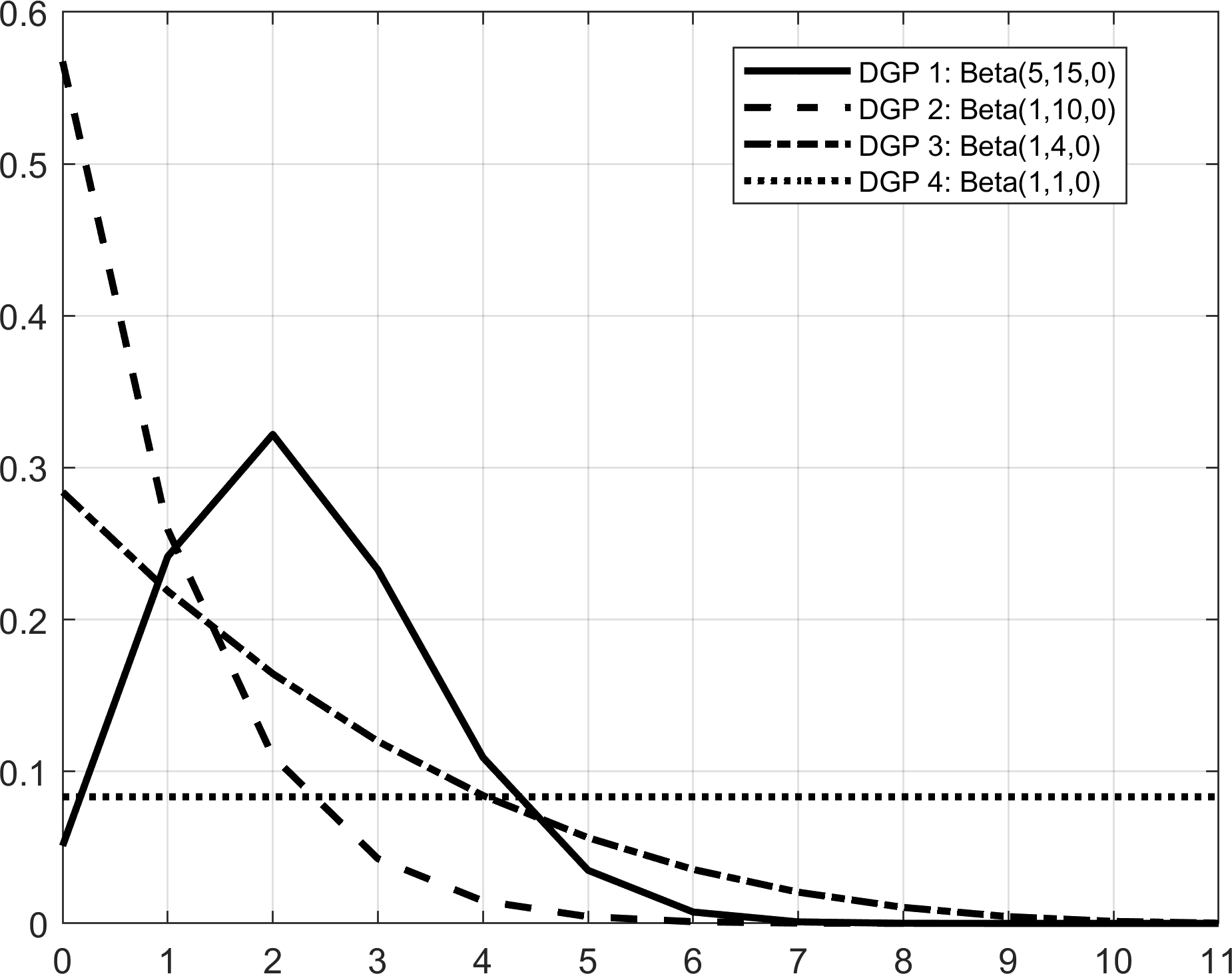
where (which is akin to a quarterly-monthly process) and . We set the true weighting scheme by relying on a three-parameters Beta function:
Figure 1: MIDAS weights in the Monte Carlo simulations
We investigate four alternative weighting schemes that correspond to bell-shaped weights (DGP 1) with , fast-decaying weights (DGP 2) with , slow-decaying weights (DGP 3) with , and flat weights (DGP 4) with . These weighting schemes are represented in Figure 1.555The weights are set to exactly zero for values of the Beta function , and normalized to sum up to 1.
Note that the same weighting scheme applies to all the predictors entering the DGPs. We define and as i.i.d. draws from the following multivariate distribution:
where , with a diagonal matrix with elements and a Toeplitz correlation matrix with diagonal elements equal to one and off-diagonal elements for all . We set , , , . The active set has cardinality and the indices of active variables are fixed realizations of random draws without replacement from . Conditional on these parameters, we calibrate such that the noise-to-signal ratio of the mixed-frequency regression is for all the simulations. We assume (akin to a nowcasting model). The number of in- and out-of-sample observations is again fixed at and , respectively.
Table 4: Monte Carlo simulations: selection and predictive accuracy
DGP 1
DGP 2
DGP 3
DGP 4
bell-shaped
fast-decaying
slow-decaying
flat
Polynomial
TPRN
CRPS
TPRN
CRPS
TPRN
CRPS
TPRN
CRPS
50
5
Unrestricted
99.8
0.71
100.0
0.67
99.2
0.75
70.5
0.88
(0.2)
(0.01)
(0.0)
(0.01)
(0.5)
(0.01)
(3.3)
(0.01)
Almon
84.3
0.75
81.8
0.75
85.0
0.77
94.8
0.77
(0.7)
(0.01)
(1.2)
(0.01)
(0.8)
(0.01)
(0.8)
(0.01)
Restr. Almon
99.5
0.70
87.5
0.71
98.8
0.71
100.0
0.79
(0.3)
(0.01)
(0.7)
(0.01)
(0.4)
(0.01)
(0.0)
(0.01)
Legendre
86.7
0.77
86.2
0.77
84.8
0.78
98.3
0.75
(0.7)
(0.01)
(0.9)
(0.01)
(1.1)
(0.01)
(0.5)
(0.01)
Bernstein
99.3
0.71
97.2
0.67
100.0
0.70
90.8
0.84
(0.3)
(0.01)
(0.6)
(0.01)
(0.0)
(0.01)
(2.2)
(0.01)
Chebychev T
87.5
0.76
81.7
0.76
84.0
0.78
98.7
0.75
(0.7)
(0.01)
(1.2)
(0.01)
(1.3)
(0.01)
(0.5)
(0.01)
100
5
Unrestricted
99.3
0.72
99.2
0.69
98.2
0.74
42.2
0.94
(0.5)
(0.01)
(0.5)
(0.01)
(0.9)
(0.01)
(2.8)
(0.01)
Almon
83.3
0.77
78.8
0.79
81.8
0.79
91.3
0.80
(0.3)
(0.01)
(1.5)
(0.01)
(1.1)
(0.01)
(1.1)
(0.01)
Restr. Almon
97.3
0.71
83.5
0.74
94.8
0.71
93.7
0.83
(0.6)
(0.01)
(0.2)
(0.01)
(0.8)
(0.01)
(1.4)
(0.01)
Legendre
80.2
0.79
82.7
0.81
78.3
0.81
91.0
0.78
(1.2)
(0.01)
(1.5)
(0.01)
(1.7)
(0.01)
(2.1)
(0.01)
Bernstein
98.7
0.72
94.5
0.69
99.3
0.70
66.8
0.89
(0.6)
(0.01)
(0.8)
(0.01)
(0.6)
(0.01)
(3.3)
(0.01)
Chebychev T
80.3
0.79
81.7
0.79
78.7
0.81
91.7
0.78
(1.3)
(0.01)
(1.0)
(0.01)
(1.6)
(0.01)
(1.8)
(0.01)
100
10
Unrestricted
23.3
0.96
27.9
0.93
16.1
0.98
10.1
0.99
(2.1)
(0.01)
(2.7)
(0.01)
(1.3)
(0.01)
(0.3)
(0.00)
Almon
20.8
0.98
10.6
0.99
21.7
0.98
25.5
0.96
(2.6)
(0.01)
(0.7)
(0.00)
(2.6)
(0.01)
(3.1)
(0.01)
Restr. Almon
88.2
0.77
89.3
0.76
87.4
0.78
17.7
0.97
(2.0)
(0.01)
(1.1)
(0.01)
(2.3)
(0.01)
(1.0)
(0.00)
Legendre
16.5
0.98
14.2
0.98
18.6
0.97
16.2
0.98
(1.7)
(0.01)
(0.6)
(0.00)
(2.1)
(0.01)
(2.2)
(0.01)
Bernstein
17.1
0.98
62.0
0.80
20.4
0.95
10.5
0.99
(0.9)
(0.01)
(3.6)
(0.02)
(2.1)
(0.01)
(0.4)
(0.00)
Chebychev T
19.1
0.97
10.8
0.99
19.1
0.98
13.1
0.98
(2.0)
(0.01)
(0.4)
(0.00)
(2.3)
(0.00)
(1.5)
(0.00)
Notes: TPR and CRPS denote respectively the true positive rate and the continuously ranked probability score, the latter in relative terms with respect to the AR(1) benchmark. Average values across Monte Carlo simulations. Bootstrap standard errors in parentheses.
In the simulations, we consider and evaluate a set of alternative approximating functions for the true weighting function , leading to the family of lag polynomials presented in Section 2.3.2: the U-MIDAS (Foroni et al., 2015), Almon lag polynomials (restricted and unrestricted; Mogliani and Simoni, 2021), and orthogonal lag polynomials. As for the latter, we consider Legendre and Chebychev (first kind) polynomials, and we introduce the Bernstein orthogonal polynomials.666For the Almon lag polynomials, we consider both unrestricted and restricted parameterizations, with truncation of the polynomial at and endpoint restrictions tailored to constrain the weighting function to tail off slowly to zero (Mogliani and Simoni, 2021). The Legendre, Chebychev, and Bernstein polynomials are normalized and shifted on , and we fix the truncation parameter at . Results for the Chebychev second kind polynomial, very close to those for the first kind polynomial, are available upon request. See Section 2.3.2 for more details.
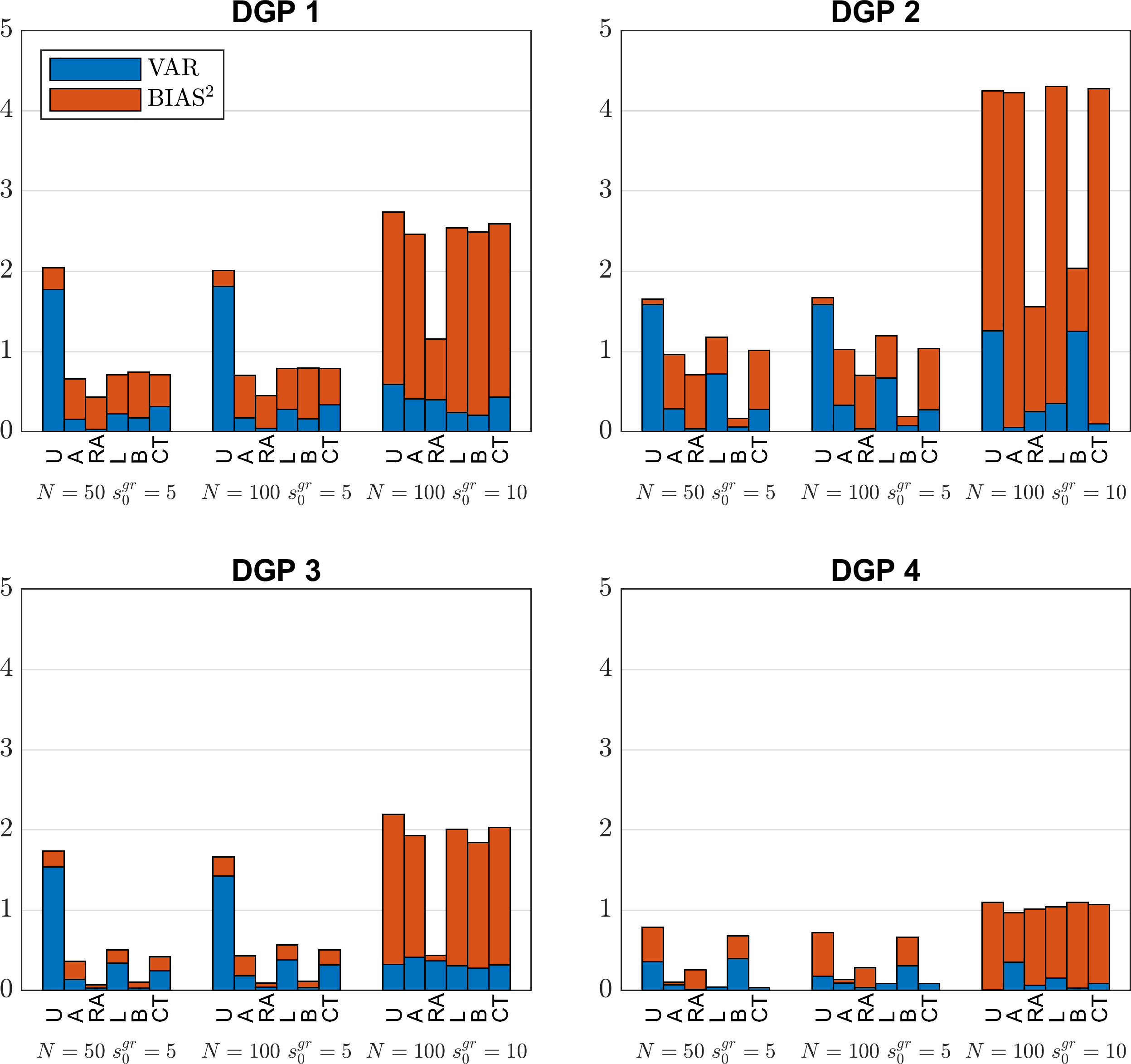
Simulation results are reported in Tables 4. We focus on the selection and predictive accuracy performance of the BGSS-SS prior in the MIDAS framework by computing the True Positive Rate (TPR) and the continuously ranked probability score (CRPS). The results point to a number of interesting features. First, among the lag polynomials considered, the best results are provided by the unrestricted, the restricted Almon and the Bernstein polynomials. Legendre polynomials, recently proposed by Babii et al. (2022) in the MIDAS framework, is often outranked by the other polynomials in our analysis. Second, consistently with the theory, the results for the best-performing polynomials seems overall unaltered by the increase in the total number of high-frequency predictors. However, the performance is substantially affected by the increase in the number of true active variables. In this case, the restricted Almon performs surprisingly better than the other polynomials, which show, for some DGPs, very low selection and predictive accuracy. Third, the ranking of the best-performing polynomials may depend, at least in part, on the shape of the underlying true weighting function. For instance, the restricted Almon seems well suited for bell-shaped and slow-decaying weights, but somewhat less for fast-decaying weights, while unrestricted and Bernstein polynomials can perform fairly well irrespective of the underlying weighting structure. However, as illustrated by the MSE in Figure 15, the U-MIDAS provides systematically less accurate parameter estimates (due mostly to a larger variance component) compared to restricted Almon and Bernstein polynomials. Interestingly enough, the performance of Legendre and Chebychev (first kind) polynomials improves substantially under flat weights. This weighting structure is nevertheless less likely to describe the actual temporal aggregation for most economic data.
Figure 2: MSE in the Monte Carlo simulations
Notes: The labels denote the Unrestricted MIDAS (U), the Almon lag polynomials (A), the Restricted Almon lag polynomials (RA), the Legendre polynomials (L), the Bernstein polynomials (B), and the Chebychev first kind polynomials (CT).
7 Empirical application: nowcasting US GDP in a mixed-frequency framework
We use the proposed prior for a nowcasting exercise of US GDP in the following mixed-frequency framework:
(39)
where is the annualized quarterly growth rate of GDP, and is a vector of macroeconomic series sampled at monthly frequency and extracted from the FRED-MD database (McCracken and Ng, 2016). The data sample starts in 1980Q1, while the pseudo out-of-sample analysis spans 2013Q1 to 2022Q4. Estimates are carried-out recursively using a rolling window of quarterly observations, and -step-ahead posterior predictive densities are generated from (38) through a direct forecast approach. We consider 3 nowcasting horizons () and the two lag polynomials – namely the restricted Almon and the orthonormal Bernstein polynomials – that provide overall better results in the simulation analysis reported in Section 6.2. Further, as the considered data sample spans periods characterised by strong and uneven macroeconomic fluctuations (permanent and transitory), such as the Great Moderation, the Great Recession, and the Covid crisis, we also allow for time-varying volatility with heavy tails and occasional outliers in the regression errors (see Section 5.2). Finally, it is worth noting that the empirical application does not take into account real-time issues (ragged/jagged-edge data and revisions) and the data used for the analysis reflect the latest vintages available at the time of writing.777The GDP series used in the analysis was downloaded from FRED on July 2023. Further, we considered the 2023-06 vintage of the FRED-MD database. For the latter, we excluded from the analysis 5 series presenting sampling issues over the time span considered for the analysis (namely, new orders for consumer goods, non-borrowed reserves of depository institutions, 3-month AA financial commercial paper rate, 3-month commercial paper minus fed funds, consumer sentiment index).
We consider several modelling strategies to exploit our bi-level sparsity prior approach. First, we estimate the forecasting model on the whole set of 122 indicators. Depending on the lag polynomial, the total number of parameters is hence either 244 (restricted Almon) or 732 (Bernstein). However, the simulation results reported in Section 6 point to a substantial deterioration of the selection and prediction performance of our prior in extreme sparse settings where . To attenuate this issue, we consider also an alternative strategy based on estimating the model on separate groups of indicators, where the groups are set according to partition of indicators defined in McCracken and Ng (2016). We hence consider a total number of 8 groups (output and income; labour market; housing; consumption, orders, and inventories; money and credit; interest and exchange rates; prices; stock market), each one including a subset of indicators, whose number ranges between 5 and 31. Summing up, we estimate a large set of alternative specifications, according to the 2 lag polynomials (Almon and Bernstein), the 5 volatility process (homoskedastic, SV, SV with Student- shocks, SV with outliers, SV with Student- shocks and outliers), and the 2 partition strategies (whole dataset vs 8 groups).888From (26), the stochastic volatility process without fat tails and/or occasional outliers implies a degenerate posterior distribution at value 1 for and/or .
To process this large amounts of results, we combine along several dimensions the set of individual density forecasts obtained:
1.
Pooling the groups: for each permutation of lag polynomials and volatility processes, we pool the forecasts obtained for the 8 groups of indicators. We then obtain 10 distinct pools of forecasts.
2.
Pooling the volatility processes (groups): from step 1), for each lag polynomial, we pool the 5 set of combined forecasts arising from the different volatility processes (groups). We then obtain 2 distinct pools of forecasts.
3.
Pooling the lag polynomials and the volatility processes: we pool the 10 set of combined forecasts from step 1).
4.
Pooling the volatility processes (whole dataset): for each lag polynomial, we pool the 5 set of combined forecasts arising from the different volatility processes and obtained from estimates on the whole dataset. We then obtain 2 distinct pools of forecasts.
5.
Pooling the lag polynomials and the volatility processes (whole dataset): we pool the 10 set of combined forecasts obtained from estimates on the whole dataset.
We have then a total number of 16 pools of forecasts. The combination is carried out using the optimal prediction pool proposed by Geweke and Amisano (2011), which relies on log-scores. The combined point and density forecasts are then evaluated by the means of standard criteria (RMSFE and average CRPS0.
Table 5: Empirical results: nowcasting US GDP
BSGS-SS
BSGL
Panel A. RMSFE
Groups - Almon
0.78
0.79
0.73
0.77
0.78
0.74
(0.11)
(0.09)
(0.03)
(0.20)
(0.07)
(0.02)
Groups - Bernstein
0.66
0.70
0.77
0.71
0.75
0.74
(0.04)
(0.01)
(0.06)
(0.08)
(0.01)
(0.04)
Groups - all
0.68
0.70
0.74
0.69
0.75
0.75
(0.04)
(0.01)
(0.04)
(0.08)
(0.01)
(0.03)
Whole dataset - Almon
0.68
0.80
0.71
0.80
0.77
0.79
(0.05)
(0.13)
(0.03)
(0.30)
(0.05)
(0.03)
Whole dataset - Bernstein
0.67
0.72
0.86
0.90
1.04
0.90
(0.05)
(0.06)
(0.08)
(0.53)
(0.83)
(0.19)
Whole dataset - all
0.67
0.78
0.72
0.91
0.91
0.91
(0.06)
(0.11)
(0.03)
(0.56)
(0.36)
(0.20)
Panel B. CRPS
Groups - Almon
0.78
0.81
0.76
0.82
0.81
0.77
(0.02)
(0.02)
(0.00)
(0.16)
(0.02)
(0.00)
Groups - Bernstein
0.70
0.70
0.79
0.77
0.73
0.76
(0.01)
(0.00)
(0.02)
(0.04)
(0.00)
(0.00)
Groups - all
0.71
0.69
0.77
0.77
0.74
0.78
(0.01)
(0.00)
(0.01)
(0.04)
(0.00)
(0.01)
Whole dataset - Almon
0.71
0.81
0.75
0.81
0.77
0.79
(0.01)
(0.06)
(0.00)
(0.23)
(0.01)
(0.00)
Whole dataset - Bernstein
0.71
0.75
0.83
0.85
0.89
0.86
(0.01)
(0.01)
(0.03)
(0.27)
(0.35)
(0.07)
Whole dataset - all
0.70
0.78
0.76
0.85
0.84
0.87
(0.01)
(0.03)
(0.00)
(0.30)
(0.05)
(0.08)
Notes: BSGS-SS denotes the proposed bi-level sparsity prior. BSGL denotes the Bayesian Sparse Group Lasso prior (Xu and Ghosh, 2015). RMSFE and CRPS denote respectively the root mean squared forecast error and the continuously ranked probability score, in relative terms with respect to the AR(1) benchmark. -values of a test of unconditional predictive accuracy (Giacomini and White, 2006) with respect to the AR(1) benchmark in parentheses. The analysis is carried out after excluding the observations for 2020Q1, 2020Q2, and 2021Q1, for which we observe extremely large forecast errors in relation with the COVID-19 shock. Bold numbers denote the best outcomes across horizons and models.
Results are reported in Table 5 and refer to relative scores with respect to the AR(1) benchmark. Three main findings can be outlined. First, Bernstein polynomials provide accurate point and density forecast for and , but the restricted Almon performs best at . This outcome can be due to the shapes the different polynomials may assume and the way they best describe the underlying weighting structure at each horizon. However, while a combination of Bernstein and Almon tends to represent a good compromise in terms of accuracy across all the selected horizons, pooling these lag polynomials does not seem to provide here a systematic optimal strategy. Second, there is no clear-cut evidence in favour of a particular partition strategy. For and , models including the whole set of indicators seem to perform better, or very closely, to those based on groups. Conversely, pooled forecasts from models based on group partitions tend to outperform for . Overall, and consistently with the simulation results reported in Section 6.2, this outcome suggests that the proposed procedure is robust to the presence of a large number of predictors. Finally, when compared to the Bayesian Sparse Group Lasso (BSGL) prior of Xu and Ghosh (2015) (right hand side of Table 5), the results suggest that our prior can perform considerably better in terms of both point and density forecasts. Even though the outperformance is not systematically and significantly clear-cut across the whole set of results, our findings point to substantial predictive gains for some horizons and pooling strategies.
8 Concluding remarks
We propose a Bayesian approach for estimating bi-level sparse mean regression models in a high-dimensional framework, where a group structure arises from the dataset or is imposed for modelling purpose. Our hierarchical prior induces bi-level sparsity, i.e. among and within groups. We add to the existing literature by establishing frequentist asymptotic properties for our procedure in-sample and out-of-sample. Remarkably, under some mild conditions, our procedure is demonstrated to be minimax-optimal. Further, contrarily to alternative approaches, our procedure does not require orthogonality among covariates belonging to different groups. Finally, we show that a more general error structure, such as stochastic volatility and ARMA, can be accommodate by only slightly modifying the proposed prior.
Monte Carlo experiments, designed to investigate the performance of our procedure under either grouped or mixed-frequency data frameworks, point to good estimation, selection, and prediction accuracy in a fairly high sparsity setting. When applied to a nowcasting exercise of the U.S. quarter-on-quarter GDP growth with 122 indicators sampled at monthly frequencies, our procedure provides good predictive performance (in terms of point and density forecast) compared to the AR(1) and the Bayesian Sparse Group Lasso.
—————–
References
Andreou et al. (2013)
Andreou, E., Ghysels, E., Kourtellos, A., 2013. Should macroeconomic
forecasters use daily financial data and how? Journal of Business & Economic
Statistics 31 (2), 240–251.
Azzalini and Capitanio (2014)
Azzalini, A., Capitanio, A., 2014. The Skew-Normal and Related Families.
Institute of Mathematical Statistics Monographs. Cambridge (UK): Cambridge
University Press.
Babii et al. (2022)
Babii, A., Ghysels, E., Striaukas, J., 2022. Machine learning time series
regressions with an application to nowcasting. Journal of Business &
Economic Statistics 40 (3), 1094–1106.
Banbura et al. (2010)
Banbura, M., Giannone, D., Reichlin, L., 2010. Large Bayesian vector auto
regressions. Journal of Applied Econometrics 25 (1), 71–92.
Belloni et al. (2014)
Belloni, A., Chernozhukov, V., Hansen, C., 2014. High-dimensional methods and
inference on structural and treatment effects. Journal of Economic
Perspectives 28 (2), 29–50.
Bickel et al. (2009)
Bickel, P. J., Ritov, Y., Tsybakov, A. B., 2009. Simultaneous analysis of
Lasso and Dantzig selector. Annals of Statistics 37 (4), 1705–1732.
Bitto and Fruhwirth-Schnatter (2019)
Bitto, A., Fruhwirth-Schnatter, S., 2019. Achieving shrinkage in a time-varying
parameter model framework. Journal of Econometrics 210 (1), 75–97.
Cai et al. (2022)
Cai, T. T., Zhang, A. R., Zhou, Y., 2022. Sparse Group Lasso: Optimal sample
complexity, convergence rate, and statistical inference. IEEE Transactions on
Information Theory 68 (9), 5975–6002.
Carriero et al. (2015)
Carriero, A., Clark, T. E., Marcellino, M., 2015. Real-time nowcasting with a
Bayesian mixed frequency model with stochastic volatility. Journal of the
Royal Statistical Society: Series A (Statistics in Society) 178 (4),
837–862.
Carriero et al. (2019)
Carriero, A., Clark, T. E., Marcellino, M., 2019. Large Bayesian vector
autoregressions with stochastic volatility and non-conjugate priors. Journal
of Econometrics 212 (1), 137–154.
Carriero et al. (in press)
Carriero, A., Clark, T. E., Marcellino, M., Mertens, E., in press. Addressing
COVID-19 outliers in BVARs with stochastic volatility. The Review of
Economics and Statistics.
Castillo et al. (2015)
Castillo, I., Schmidt-Hieber, J., Van der Vaart, A., 2015. Bayesian linear
regression with sparse priors. The Annals of Statistics 43 (5), 1986–2018.
Chan and Hsiao (2014)
Chan, J. C. C., Hsiao, C., 2014. Estimation of stochastic volatility models
with heavy tails and serial dependence. In: Jeliazkov, I., Yang, X.-S.
(Eds.), Bayesian Inference in the Social Sciences. John Wiley & Sons,
Hoboken, New Jersey, pp. 159–180.
Chen et al. (2016)
Chen, R.-B., Chu, C.-H., Yuan, S., Wu, Y. N., 2016. Bayesian sparse group
selection. Journal of Computational and Graphical Statistics 25 (3),
665–683.
Chib (1995)
Chib, S., 1995. Marginal likelihood from the Gibbs output. Journal of the
American Statistical Association 90 (432), 1313–1321.
Chib and Jeliazkov (2001)
Chib, S., Jeliazkov, I., 2001. Marginal likelihood from the
Metropolis–Hastings output. Journal of the American Statistical
Association 96 (453), 270–281.
Clark (2011)
Clark, T. E., 2011. Real-time density forecasts from Bayesian vector
autoregressions with stochastic volatility. Journal of Business & Economic
Statistics 29 (3), 327–341.
Ferrara and Simoni (2022)
Ferrara, L., Simoni, A., 2022. When are Google Data useful to nowcast GDP?
an approach via preselection and shrinkage. Journal of Business & Economic
Statistics 41 (4), 1188–1202.
Foroni et al. (2015)
Foroni, C., Marcellino, M., Schumacher, C., 2015. Unrestricted mixed data
sampling (MIDAS): MIDAS regressions with unrestricted lag polynomials.
Journal of the Royal Statistical Society: Series A (Statistics in Society)
178 (1), 57–82.
Geweke and Amisano (2011)
Geweke, J., Amisano, G., 2011. Optimal prediction pools. Journal of
Econometrics 164 (1), 130–141.
Ghysels et al. (2006)
Ghysels, E., Santa-Clara, P., Valkanov, R., 2006. Predicting volatility:
getting the most out of return data sampled at different frequencies. Journal
of Econometrics 131 (1-2), 59–95.
Ghysels et al. (2007)
Ghysels, E., Sinko, A., Valkanov, R., 2007. MIDAS regressions: Further
results and new directions. Econometric Reviews 26 (1), 53–90.
Giacomini and White (2006)
Giacomini, R., White, H., 2006. Tests of conditional predictive ability.
Econometrica 74 (6), 1545–1578.
Hoffmann et al. (2015)
Hoffmann, M., Rousseau, J., Schmidt-Hieber, J., 2015. On adaptive posterior
concentration rates. The Annals of Statistics 43 (5), 2259 – 2295.
Lenza and Primiceri (2022)
Lenza, M., Primiceri, G. E., 2022. How to estimate a vector autoregression
after March 2020. Journal of Applied Econometrics 37 (4), 688–699.
Li et al. (2022)
Li, Z., Zhang, Y., Yin, J., 2022. Minimax rates for high-dimensional double
sparse structure over -balls. arXiv:2207.11888.
McCracken and Ng (2016)
McCracken, M. W., Ng, S., 2016. FRED-MD: A monthly database for macroeconomic
research. Journal of Business & Economic Statistics 34 (4), 574–589.
Moench et al. (2013)
Moench, E., Ng, S., Potter, S., 12 2013. Dynamic Hierarchical Factor Models.
The Review of Economics and Statistics 95 (5), 1811–1817.
Mogliani and Simoni (2021)
Mogliani, M., Simoni, A., 2021. Bayesian MIDAS penalized regressions:
Estimation, selection, and prediction. Journal of Econometrics 222 (1, Part
C), 833–860.
Ning et al. (2020)
Ning, B., Jeong, S., Ghosal, S., 2020. Bayesian linear regression for
multivariate responses under group sparsity. Bernoulli 26 (3), 2353–2382.
Raskutti et al. (2011)
Raskutti, G., Wainwright, M. J., Yu, B., 2011. Minimax rates of estimation for
high-dimensional linear regression over -balls. IEEE Transactions on
Information Theory 57 (10), 6976–6994.
Spiegelhalter et al. (2002)
Spiegelhalter, D. J., Best, N. G., Carlin, B. P., Van Der Linde, A., 2002.
Bayesian measures of model complexity and fit. Journal of the Royal
Statistical Society Series B: Statistical Methodology 64 (4), 583–639.
Stock and Watson (2016)
Stock, J. H., Watson, M. W., 2016. Core inflation and trend inflation. The
Review of Economics and Statistics 98 (4), 770–784.
Xu and Ghosh (2015)
Xu, X., Ghosh, M., 2015. Bayesian variable selection and estimation for Group
Lasso. Bayesian Analysis 10 (4), 909–936.
Zhang et al. (2020)
Zhang, B., Chan, J. C. C., Cross, J. L., 2020. Stochastic volatility models
with ARMA innovations: An application to G7 inflation forecasts.
International Journal of Forecasting 36 (4), 1318–1328.
Appendix
Appendix A Proofs of the main results
Recall the notation , .
For a vector , where for every : let denote the set of indices of the groups in a with at least one nonzero component, denote the number of groups in a with at least one nonzero component. If , for every let be the set of the indices of the nonzero elements in and . If , then while if , then . Corresponding to the true value , there are true , , for every , and .
For every , let us consider the set of associated with a group structure (defined through the inverse of the operator and the corresponding matrix as described in Section 2.2) that have less than active groups (that is, non-zero columns of the associated matrix ) and less than non-zero components:
where and are two positive constants.
Let (resp. ) denote the true (resp. the true truncated) conditional distribution of given X and the true values of the parameters (resp. ) and , and let (resp. ) denote its Lebesgue density. Moreover, and denote the Lebesgue density of the conditional distributions and , respectively, given X and generic values of the parameters , and . Let and . For a constant , the constant in Assumption 4.2, and , define the sieves:
(A.1)
where .
For two probability densities and , the Kullback-Leibler (KL) divergence is denoted by while denotes the KL variation. The average Rényi divergence of order between two -dimensional densities and is denoted by and defined as .
The proof of this theorem is divided into two parts. In the first part we obtain the posterior contraction rate with respect to . In the second part we use this result to show the statement of the theorem.
For and as defined above, let us consider the set with constants and that do not depend on and that are such that with the constant in Lemma B.3.2 in the Online Appendix that satisfies (B.3.11) and that depends only on , and the constants in Assumption 4.3. For every let . Since the prior puts mass zero on , then for every :
(A.2)
The second term on the right hand side goes to zero by Lemma B.3.3 in the Online Appendix. We then focus on the first term. By Lemma B.3.4 in the Online Appendix there exists a test such that for some constant that does not depend on ,
(A.3)
Hence, by using the first upper bound in (A.3) we get the upper bound:
(A.4)
and we just need to upper bound the second term in (A.4). To do this and for the constant introduced above, define the event , where denotes the prior in (10) - (13) marginalized with respect to the prior of and restricted to have support on . By using the results of Lemma B.3.1 with and of Lemma B.3.2 in the Online Appendix we obtain that for large :
(A.5)
Moreover, let where is as defined in (A.1) with and remark that . Then, by letting , where is the constant in the statement of the theorem, we get:
(A.6)
by using the second upper bound in (A.3) and result (B.3.32) of Lemma B.3.4 in the Online Appendix with . By putting together (A.2) and (A.4)-(A.6) and by Lemma B.3.3 we obtain:
(A.7)
which converges to zero for the values of , , and specified above. Finally, since all the constants in the right hand side of (A.7) do not depend on we conclude that
(A.8)
We now develop the second part of the proof where we use the notation . Denote . Under Assumption 4.1(i) this event is feasible. On : . Then, on :
By (A.16), the inequality , and Assumption 2.1 we get
which converges to zero by Theorem 4.1 for every such that and by Lemma B.3.3 in the Online Appendix. This shows result (17) in the theorem.
To show result (17), we lower bound the right hand side in (A.15) by ,
where we use and with probability approaching one as stated in the theorem. The remaining of the proof proceeds similarly as above.
Appendix B Online Appendix
The Online Appendix contains: guidelines for setting some hyperparameters, the MCMC algorithm for the extended model with ARMA errors and stochastic volatility, and the proofs of technical results.