Entropic pulling and diffusion diode

Abstract

Biological environments at micrometer scales and below are often crowded, and experience incessant stochastic thermal fluctuations. The presence of membranes/pores, and multiple biological entities in a constricted space can make the damping/diffusion inhomogeneous. This effect of inhomogeneity is presented by the diffusion becoming coordinate-dependent. In this paper, we analyze the consequence of inhomogeneity-induced coordinate-dependent diffusion on Brownian systems in thermal equilibrium under the Itô’s interpretation. We argue that the presence of coordinate-dependent diffusion under Itô’s formulation gives rise to an effective diffusion potential that can have substantial contribution to system’s transport. Alternatively, we relate this to the existence of an emergent force of entropic origin that dictates the transport near interfaces.

Many biological systems operate at low Reynolds numbers, where viscous forces are of paramount importance. Viscous/damping forces dominate over inertial forces and govern the mechanics of many biological systems in this regime [1, 2, 3]. Coordinate-dependent damping/diffusion is recently identified to have crucial role to play in the functioning of various biological systems [4, 5, 6, 7, 8, 9] and a lot remains to be explored. Earlier experiments by Faucheux et al, and others have proven the existence of coordinate-dependent damping [7, 8, 10] of a Brownian particle near interfaces. Ample theoretical/computational studies have been focusing on understanding systems with coordinate-dependent diffusion/damping as opposed to the uniform one [11, 12, 13, 14, 15, 16] under varied circumstances.

Translocation of proteins across cellular membranes is a central and essential process in biological systems. Molecular chaperones are macromolecules present in cells that assist these proteins to unfold, move across membranes/channels, prevent protein aggregation and help in maintaining proper functioning and health of the cell. Broadly, three mechanisms have been proposed in the literature to explain chaperone-assisted translocation of proteins: power-stroke, Brownian-ratchet and entropic-pulling [17, 18, 19, 20, 21, 22, 23, 24, 25, 26, 27]. In the power-stroke mechanism, the linkage of incoming protein with the chaperone and assistance from ATP hydrolysis induces a conformation change within chaperone that drives the protein in forward direction through the channel/pore. The Brownian-ratchet mechanism is a biased diffusion model effectively based on the idea that while passing through a pore/channel, the large size of the chaperone only allows the Brownian motion of protein-bound chaperone in one direction.

On the contrary, the entropic pulling mechanism is a thermodynamic description based on the idea that the system would try to move in a direction so as to attain a higher entropy configuration [28, 29, 30]. It is generally understood in existing literature that, in chaperone-assisted protein translocation, the tethering of protein to chaperone in the vicinity of the pore/membrane corresponds to a low entropy state. The chaperone-linked protein system via collisions with the membrane/pore generates a net effective pulling force that takes it away from pore/membrane to a region of more freedom in conformations. This constitutes an effective force transitioning to a higher entropy state.

Entropic-pulling of a meso-scale object from open space to a narrower one is beyond any scope under homogeneous diffusion making such a phenomenon counter-intuitive. In the present paper, we are going to illustrate effects of a new source of entropy arising out of coordinate-dependent diffusion [31]. The presence of this entropy eventually could give rise to an entropic-force which could drag a Brownian particle or a mesoscopic object towards a region of higher damping despite the region of higher damping being a relatively constricted space. In general, coordinate-dependent diffusion is a hydrodynamic effect, where a Brownian particle experiences enhanced damping near an interface or wall than that it undergoes in the bulk. This makes the particle spend more time near a wall compared to that in the bulk and this phenomenon can be understood in terms of this new inhomogeneity-entropy arising out of coordinate dependence of diffusion. We demonstrate working of this entropic-force, in the present paper, in two classes of phenomenon. These two phenomena are (1) diffusion-diode and (2) chain-pulling through a pore.

In the absence of coordinate-dependent diffusion, diffusive transport is always driven by concentration gradients. However, in the presence of diffusivity gradient, the gradient can force a diffusive transport even against concentration gradient. If one imagines that the concentration gradient is representing a driving field for current in the presence of coordinate dependent diffusion, then, until this driving force overcomes the barrier of the diffusion gradient it will not be able to cause substantial transport in its direction. This, however, is not the case when the concentration gradient and the diffusion gradient are in the same direction. The operating principle of a diffusion-diode would be based on cooperation/opposition of these two gradients and can be realized in the presence of coordinate dependence of diffusion.

In equilibrium, diffusivity and damping are inversely related by fluctuation-dissipation relation. As a result, diffusivity decreases near a wall due to increase in damping. This decrease in diffusivity creates a higher entropy region near a wall compared to that in the bulk. Therefore, there always be a tendency in the diffusive transport of macro-molecules to make them get attracted towards a wall/pore near which this entropy is higher.

Due to this same effect, a chain-like macro-molecule left to meander under equilibrium thermal fluctuations would eventually move from a wider region of space to a nearby narrower one under the action of coordinate-dependent diffusion. To our knowledge, possibility of occurrence of this phenomenon has not been paid attention to due mostly to not having considered the Itô-process as an equilibrium scenario for coordinate-dependent diffusion. These are novel phenomena possible under coordinate-dependent diffusion which might hold the key for understanding complex biological systems in a substantially new way.

The paper is organized in the following manner: the first section revisits basics of an Itô-process using Fokker-Planck equation and demonstrates how a force of entropic origin emerges therein. Subsequently, we introduce a simple model to demonstrate the working of a diffusion-diode. This is followed by a section on entropic-pulling based translocation of a chain-like molecule through a pore. The paper is concluded by discussing implications of inhomogeneity-entropy arising due to coordinate-dependent damping/diffusion in the context of biological systems.

I Coordinate-dependent diffusion

Stochastic modeling has played an eminent role in helping biologists and physicists understand various natural phenomena [32, 33, 34, 35] like the directed motion of molecular motors, the spread of epidemics, gene regulation etc. The evolution of such stochastic systems are often understood by expressing the dynamics as a partial differential equation in the presence of a thermal noise. In one spatial dimension $x$, an Itô-process is governed by the following Fokker-Planck equation [36, 16]:

$$\frac{\partial}{\partial t}p(x,t) = -\frac{\partial}{\partial x}[\nu(x)p(x,t)]+\frac{\partial^{2}}{\partial x^{2}}[D(x)p(x,t)].$$

where $p(x,t)$ is the probability density of the particle at position $x$ and time $t$, $\nu(x)=\frac{F(x)}{\Gamma(x)}$ is the drift velocity (coefficient) and $D(x)$ is the diffusion coefficient. The deterministic (conservative) force on the particle being $F(x)$, the damping coefficient is denoted by $\Gamma(x)$ which, in general, is related to the diffusivity in the time-independent case as $\Gamma(x)=\frac{k_{B}T}{D(x)}$ by the fluctuation-dissipation relation under local equilibrium conditions at temperature $T$ with $k_{B}$ being the Boltzmann constant. The Fokker-Planck equation is a continuity equation for conserved probability.

$$\frac{\partial}{\partial t}p(x,t) = -\frac{\partial}{\partial x}J(x,t).$$

where $J(x,t)$ is the probability current density, with $J(x,t)=\nu(x)p(x,t)-\frac{\partial}{\partial x}D(x)p(x,t)$. The first term here corresponds to drift current density and second term to diffusion current density [37, 38, 39, 40, 36, 16, 41, 42, 31]. Now, for a stationary distribution in equilibrium $J^{eq}(x)=0$ (condition for detailed balance), the following equilibrium distribution $p^{eq}(x)$ results:

$$p^{eq}(x)=C\frac{D_{0}}{D(x)}\exp\left(\int dx\frac{\nu(x)}{D(x)}\right).$$

Here $C$ is a constant with dimensions of inverse length, and $D_{0}$ is a constant diffusivity away from any interface to which $D(x)$ converge as the Brownian particle makes its excursion to the bulk region of allowed space.

This distribution is referred to as generalized/modified Boltzmann distribution or Itô-distribution in [16, 43, 44, 41]. Now, the drift velocity $\nu(x)$ can be expressed in terms of potential $U(x)$ corresponding to a conservative force and coordinate dependent damping $\Gamma(x)$ as : $\nu(x)=-\frac{1}{\Gamma(x)}\frac{\partial}{\partial x}U(x)$. The equilibrium distribution $p^{eq}(x)$ thus becomes [42, 45, 16, 41]

$$p^{eq}(x)=C\frac{D_{0}}{D(x)}\exp\left(-\frac{U(x)}{k_{B}T}\right).$$ (1)

The presence of the coordinate-dependent diffusivity-dependent amplitude $D_{0}/D(x)$, makes all the difference and is responsible for the possibility of various interesting processes in thermal equilibrium like bath-fluctuation-driven spontaneous collective transport [45], rectified transport of symmetry broken hetero-dimer [46, 42] etc. The legitimacy of the distribution (1) as an equilibrium distribution could be illustrated by rewriting $p^{eq}(x)$ as

$$p^{eq}(x)=C\exp\left(-\frac{1}{k_{B}T}\left[U(x)-k_{B}T\log\frac{D_{0}}{D(x)}\right]\right),$$ (2)

where interpretation of the above expression could be that, the presence of coordinate dependence of diffusion generates a diffusion potential $U_{D(x)}=-k_{B}T\log\frac{D_{0}}{D(x)}$, which corresponds to a force $f_{diff}=-\frac{\partial}{\partial x}U_{D(x)}=-k_{B}T\frac{d}{dx}\log D(x)$. This force supports the motion in the direction of decreasing diffusion. This is the Molecular-kinetic/tree description in the context of the paper by Sousa and Lafer [18]. Another way to interpret this is the thermodynamic description [18, 31], where one interprets the presence of position-dependent diffusion responsible for the emergence of additional entropy. The term $\frac{D_{0}}{D(x)}$ can be interpreted as the dimensionless density of states arising in the presence of coordinate-dependent diffusion [31]. The corresponding force $f_{en}(x)=-\frac{d\mathcal{F}}{dx}=T\frac{dS}{dx}$. Here $\mathcal{F}$ corresponds to free energy. This in our case means $f_{ent}=-k_{B}T\frac{d}{dx}\log D(x)$. This force is responsible for the entropic-pulling mechanism.

II DIFFUSION DIODE

Consider a model consisting of $N$ Brownian particles confined inside a three-dimensional box in the presence of a heat bath in equilibrium at temperature $T$. Brownian particles interact with each other through excluded volume interaction in the vicinity of one another. Overdamped stochastic differential equations

$$\frac{d{\mathbf{r}_{i}}}{dt} = \frac{\mathbf{F}_{i}}{\Gamma_{i}}+\sqrt{\frac{2k_{B}T}{\Gamma_{i}}}{\bm{\eta}}_{i}(t),$$ (3)

govern such a system where $\bm{r}_{i}$ is the position coordinate of $i^{th}$ particle. $\bm{F}_{i}$ is the instantaneous force amounting to the total contribution of excluded volume interaction and the confinement felt by the $i^{th}$ particle, in case it tries to cross the boundary. $k_{B}T$ represents the thermal energy scale of the heat bath at temperature $T$. $\Gamma_{i}$ is coordinate-dependent damping coefficient assigned to the $i^{th}$ particle. Stochastic noise $\bm{\eta}_{i}(t)$ felt by $i^{th}$ particle is a three-component Gaussian white noise vector, which in Cartesian coordinate representation is $\bm{\eta}_{i}(t)={\eta}^{x}_{i}(t)\hat{{x}}+{\eta}^{y}_{i}(t)\hat{{y}}+{\eta}^{z}_{i}(t)\hat{{z}}$. Each component represents Gaussian white noise of zero mean and a unit strength. None of these components are cross-correlated i.e. $\langle\eta^{s}_{i}(t)\rangle$ = 0 and $\langle\eta^{s}_{i}(t_{1})\eta^{s^{\prime}}_{j}{(t_{2})}\rangle=\delta_{ij}\delta_{ss^{\prime}}\delta(t_{1}-t_{2})$, with $i$, $j$ $\in$ $\{1,2,\ldots\,N\}$ and $s/s^{\prime}\in\{x,y,z\}$.

We set up a box in the first octant, with the origin (0, 0, 0) coincident on one of the corners. All distances are measured from the origin. Length of the box in $y$ and $z$ directions are equal by construction. We introduce a global coordinate-dependence of damping in the box in this model. This is achieved by dividing the box into three cuboidal regions: $R_{1}$, $R_{2}$ and $R_{3}$ along $x$-axis, where regions $R_{1}$ and $R_{3}$ are geometrically identical. The damping profile is such that the damping strength is almost constant in $R_{1}$, increasing in region $R_{2}$ till it reaches region $R_{3}$, where it again saturates to another almost constant value. The damping profile chosen is a monotonically increasing, continuous, and differentiable function.

We study two cases under such a scenario:- Case I: $N$ Brownian particles are randomly placed in $R_{1}$ at the start of the simulation, and Case II: $N$ Brownian particles are randomly placed in $R_{3}$ at the start of the simulation. We allow the system of particles to evolve numerically as an Itô-process and compare the dynamics in both cases.

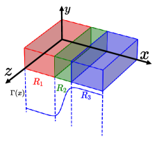
Figure 1: Set up of the model

The excluded volume interaction between different particles $i$ and $j$ is modeled by repulsive harmonic potential $V_{ij}$.

$$V_{ij}=\begin{cases}\frac{1}{2}\kappa(|\mathbf{r}_{i}-\mathbf{r}_{j}|-r_{l})^{2}&\text{if $|\mathbf{r}_{i}-\mathbf{r}_{j}|<r_{l},$}\\ \\ 0&\text{if $|\mathbf{r}_{i}-\mathbf{r}_{j}|\geq r_{l},$}\end{cases}$$

where, $\kappa$ measures the strength of repulsion, $r_{l}$ is the proximity scale below which repulsion is felt by particles. Suppose $\phi_{i}$ represents the net potential on the $i^{th}$ particle due to other particles, then $\phi_{i}=\sum\limits_{\begin{subarray}{c}j\end{subarray}}V_{ij}(1-\delta_{ij})$. $\delta_{ij}$ is the standard kronecker delta function. The corresponding force felt is $-\nabla_{\textbf{r}_{i}}\phi_{i}$. The confinement interaction is modeled by a piecewise harmonic repulsive potential. Suppose $b_{i}=\{x_{i},y_{i},z_{i}\}$ and $l_{b}=\{l_{x},l_{y},l_{z}\}$ constitute ordered pairs, where elements of $b_{i}$ represent cartesian components of $i^{th}$ particle’s position and elements of $l_{b}$ represent edge-length of the box in $x$, $y$ and $z$ direction respectively. The confining potential corresponding to each component of $b_{i}$ and $l_{b}$ is denoted by $V_{b_{i}}$.

$$V_{b_{i}}=\begin{cases}\frac{1}{2}\kappa{b}_{i}^{2}&\text{if ${b}_{i}<0,$}\\ \\ 0&\text{if $0\leq b_{i}\leq l_{b},$}\\ \\ \frac{1}{2}\kappa({b}_{i}-l_{b})^{2}&\text{if ${b}_{i}>{l_{b}}$}\end{cases}$$

The overall confining potential $V_{c}=\sum\limits_{\begin{subarray}{c}b_{i}\end{subarray}}V_{b_{i}}$. Thus, the net force felt by $i^{th}$ particle due to excluded volume and confinement effects is $\mathbf{F}_{i}=(-\nabla_{\textbf{r}_{i}}\phi_{i})+(-\nabla_{\textbf{r}_{i}}V_{c})$.

The coordinate-dependent damping is modeled by a hyperbolic tangent function in the simulations. The following functional form of damping experienced by $i^{th}$ particle, is used in simulations:

$$\Gamma_{i}=A\hskip 2.84526pt\tanh{\beta(x_{i}-x_{0})}+(A+1),$$

where $x_{0}$ is shifted origin and $A$ is amplitude parameter, where $\beta$ is the measure of the steepness of the profile in neighborhood of $x_{0}$ and effectively is a measure of region $R_{2}$ in $x$ direction. The last term in the above expression of damping accounts for vertical shifting of standard hyperbolic tangent function to ensure that damping is always positive. We have chosen $x_{0}$ to be midpoint of length of three-dimensional box in $x$ direction.

The initial configuration in case I corresponds to randomly placing all the particles in $R_{1}$. This initial placement sets up a particle concentration gradient that favors particle motion through $R_{2}$. Normal concepts of diffusion would dictate that the particles would diffuse to reach a uniform distribution. Coordinate dependence of damping sets up a diffusion potential according to the set diffusion gradient. This when evolved an Itô-process induces motion of particles in the direction of decreasing diffusivity (increasing damping) in accordance with the Itô’s framework. The combined result of the two processes is that the majority of particles diffuse to region $R_{3}$, and consequently, a steady state is reached with higher concentration in $R_{3}$.

Now, consider case II, where all the particles are randomly placed in $R_{3}$ at the start of the simulation. This assignment creates a concentration gradient favoring the motion of particles through $R_{2}$ to $R_{1}$ for normal diffusion. However, the diffusion potential as per Itô-process sets up a diffusion barrier to overcome to this concentration-driven current. Consequently, a steady state is reached at long times with most of the particles staying in $R_{3}$. This is a diode in reverse bias if one goes by the conventional idea of considering diffusion being driven by concentration gradient.

${n}_{f}$ represents the ensemble-averaged number of particles reaching $R_{3}$ starting from $R_{1}$. It corresponds to case I. Similarly ${n}_{b}$ denotes the ensemble-averaged number of particles occupying region $R_{3}$ given they start from $R_{3}$ and it corresponds to case II. It is evident from Fig.$2(a)$ (case I) that when particles are initially placed in $R_{1}$, the majority of them reach $R_{3}$ at long times. This is because the inhomogeneity-induced diffusion potential sets up a diffusion gradient which aids the concentration gradient in the motion in this (forward) direction. The situation is similar to forward biasing in a traditional diode by assistance in forward motion. In case II as evident from Fig.$2(b)$, most of the particles can’t crossover to region $R_{2}$ because the inhomogeneity-induced diffusion potential generates a diffusion gradient that opposes the motion of particle from $R_{3}$ to $R_{2}$ (backward) direction. Simulation details used here can be found in Appendix A and Appendix B.

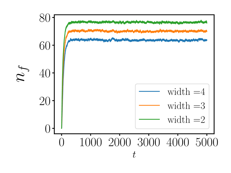
(a) Case I

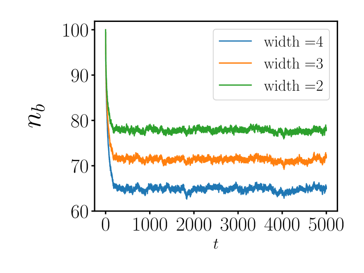
(b) Case II

Figure 2: Occupation of particles in $R_{3}$ shown for various widths of $R_{2}$ as a function of time displayed for (a) case I and (b) case II. Widths of 4, 3, and 2 correspond to the following values of $\beta$: 2.5, 3.3, and 5 respectively.

III Entropic pulling of a chain

In this section, we consider a polymer chain confined inside a three-dimensional funnel-like geometry in contact with a heat reservoir in thermal equilibrium at a temperature $T$. The polymer comprises $N$ interacting Brownian monomers. The shape of the funnel is shown in Fig.$3$. It is useful to think of the funnel as divided into three sections: $R_{1}$, $R_{2}$, and $R_{3}$, all seamlessly linked together. $R_{1}$ is a hollow right circular cylindrical region of radius $\mathcal{R}$. $R_{2}$ is a hollow truncated cone-shaped region (or frustum of a cone) with big radius $\mathcal{R}$ and small radius $r$. $R_{3}$ is a hollow right circular cylindrical region of radius $r$. All regions have equal length by construction. We establish our reference point, the origin, at the center of the rear circular base (radius $\mathcal{R}$) of the funnel, which marks the beginning of region $R_{1}$. The positive direction of $z$ axis is a ray coincident with the axis of symmetry of funnel emerging from origin towards other regions, with $x$ and $y$ axis perpendicular to $z$ axis. It is evident from the nature of geometry of the funnel that curved boundaries of regions $R_{1}$, $R_{3}$ lie at a constant radial distance from $z$ axis whereas for $R_{2}$, this distance keeps on decreasing with increasing $z$ coordinate. Thus, this geometry can be used to model the effect of the wall on diffusivity/damping on the particle.

We introduce a confining potential on boundaries to ensure that polymer stays inside the funnel. In the model, we introduce two intra-polymer interactions: (i) nearest-neighbor monomer interaction and (ii) interaction between all other pairs. The nearest neighbor monomers feel attractive interaction above an equilibrium separation and an excluded volume interaction below it. All other pairs of monomers interact via excluded volume interaction in proximity to one another. We evolve the system as an Itô process. The following equation of motion describes the dynamics of $i$-th monomer under Itô description.

$$\begin{split}\frac{d{\mathbf{r}_{i}}}{dt}&=-\frac{1}{\Gamma_{i}}\nabla_{\mathbf{r}_{i}}\Big{[}\sum\limits_{\begin{subarray}{c}j=i\pm 1\end{subarray}}V_{NN}(|\mathbf{r}_{i}-\mathbf{r}_{j}|)+\sum\limits_{\begin{subarray}{c}j\\ j\neq i,i\pm 1\end{subarray}}V_{O}(|\mathbf{r}_{i}-\mathbf{r}_{j}|)\Big{]}\\ &-\frac{1}{\Gamma_{i}}\nabla_{\mathbf{r}_{i}}V_{B}(\mathbf{r}_{i})+\sqrt{\frac{2k_{B}T}{\Gamma_{i}}}{\bm{\eta}}_{i}(t).\end{split}$$

where $i,j$ $\in$ $\{1,2,\ldots\,N\}$ are monomer indices and $\mathbf{r}_{i}$ denotes the position vector of $i^{th}$ monomer. ${r}_{ij}=|\mathbf{r}_{ij}|=|\mathbf{r}_{i}-\mathbf{r}_{j}|$ is the magnitude of separation between $i^{th}$ and $j^{th}$ monomer. $\Gamma_{i}$ is the damping coefficient associated with the $i^{th}$ monomer. $V_{NN}$ captures the interaction between monomers directly linked to one other, while $V_{O}$ accounts for the interaction between monomer that are not nearest neighbour pairs. $V_{B}$ denotes the potential that restrains the $i$-th monomer in the event it crosses funnel boundary. ${\bm{\eta}}_{i}(t)$ signifies Gaussian vector white noise experienced by $i$-th monomer possessing same statistical properties as those elucidated in the diffusion diode section.

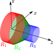
Figure 3: Funnel [not drawn to scale]

The cross-sectional radius $s$ in each region of the funnel can be expressed as:

$$s(z)=\begin{cases}\mathcal{R}&\text{if $0\leq z\leq h,$}\\ \\ {r+(2h-z)(\frac{\mathcal{R}-r}{h})}&\text{if $h\leq z\leq 2h,$}\\ \\ r&\text{if $2h\leq z\leq 3h,$}\end{cases}$$

where $h$ is each region’s length in $z$ direction. The nearest neighbor monomer interaction $V_{NN}$ is modeled by a harmonic potential.

$$V_{NN}({r}_{ij})=\frac{\alpha}{2}({r}_{ij}-r_{min})^{2},$$

where $\alpha$ is the spring constant, $r_{min}$ is the equilibrium separation and $r_{ij}$ is the separation between nearest neighbour’s $i$ and $j$, where ($j=i\pm 1$). The excluded volume interaction between the rest of monomer pairs is modeled using Weeks–Chandler–Andersen (WCA) potential and represented by $V_{O}$.

$$V_{O}({r}_{ij})=\begin{cases}4\epsilon[\frac{\sigma^{12}}{{r}_{ij}^{12}}-\frac{\sigma^{6}}{{r}_{ij}^{6}}]+\epsilon&\text{if ${r}_{ij}<2^{\frac{1}{6}}\sigma,$}\\ \\ 0&\text{if ${r}_{ij}\geq 2^{\frac{1}{6}}\sigma,$}\end{cases}$$

where, $\epsilon$ measures the depth of the standard L-J potential well, $\sigma$ is a length parameter and $r_{ij}$ is the separation between $i^{th}$ and $j^{th}$ monomer with ${j\neq i,i\pm 1}$.

The position of $i^{th}$ monomer in three-dimensional space can always be expressed in a cartesian coordinate system by three independent cartesian coordinates, {$\mathbf{r}_{i}$} $\Longleftrightarrow$ {$x_{i}$, $y_{i}$, $z_{i}$}. The presence of cylindrical symmetry in the funnel allows for a convenient representation of confining potential at the periphery and above it, in cylindrical coordinates, {$\mathbf{r}_{i}$} $\Longleftrightarrow$ {$\rho_{i}$, $\phi_{i}$, $z_{i}$}. $\rho_{i}$ symbolises the radial distance of the $i^{th}$ monomer from $z$ axis and $\phi_{i}$ expresses the azimuth angle made by $i^{th}$ monomer on $x$-$y$ plane, where $\rho_{i}=\sqrt{x_{i}^{2}+y_{i}^{2}}$ and $\phi_{i}=\tan^{-1}(\frac{y_{i}}{x_{i}})$. The funnel boundary consists of two types of surfaces: a curved cylindrical surface, directed in a direction normal to the $z$ axis, and a plane circular surface towards the rear ends of the funnel along the $z$ axis. The confinement interaction is defined separately for both surfaces but in either case, is modeled by harmonic repulsion. Suppose $\Phi_{c}$ and $\Phi_{p}$ signify the confining potentials that the $i^{th}$ monomer experiences on overshooting the curved cylindrical boundary and plane circular periphery of the funnel, respectively.

$$\Phi_{c}(\rho_{i}) =\begin{cases}0&\text{if }\rho_{i}<s_{i},\\ \\ \frac{\kappa}{2}(\rho_{i}-s_{i})^{2}&\text{if }\rho_{i}\geq s_{i}.\end{cases}$$

$$\Phi_{p}(z_{i}) =\begin{cases}\frac{\kappa}{2}(z_{i}-0)^{2}&\text{if }z_{i}\leq 0,\\ \\ 0&\text{if }0<z_{i}<3h,\\ \\ \frac{\kappa}{2}(z_{i}-3h)^{2}&\text{if }z_{i}\geq 3h.\end{cases}$$

where, $\kappa$ is measure of strength of harmonic repulsion, $s_{i}(z_{i})$ is the cross-sectional radius seen by $i^{th}$ particle corresponding to it’s $z$ coordinate, $z_{i}$. Thus, the overall confining potential $V_{B}$ becomes, $V_{B}$ = $\Phi_{c}+\Phi_{p}$.

Having described the system, in the following section, we show the effect of the presence and absence of coordinate-dependent damping on the dynamics of the polymer chain. We consider two cases. Case I corresponds to the introduction of damping dependent on $z$ coordinate, $\Gamma_{i}=A/s_{i}(z_{i})$, where $A$ is a constant. Such a choice provides uniform damping in regions $R_{1}$ and $R_{3}$ and a monotonically increasing damping as the polymer moves in region $R_{2}$ along increasing $z$ direction. In Case II , we consider a constant damping profile experienced by the monomer throughout the funnel, $\Gamma_{i}=A/R$, which equals a constant. We evolve both cases as an Itô process using simulation and compare the dynamics at the end of the simulation.

The initial state of the polymer in cases I and II is an identical unfolded linear chain conformation coincident on the $z$ axis lying in $R_{1}$ in all the ensembles. We generate independent ensembles using a different random seed and thus a different sequence of random numbers for each ensemble in case I. For case II, we generate an equal number of independent ensembles by using the same random seed and the same corresponding sequence of random numbers as for case I. After having fixed the polymer to the same initial configuration, and the same sequence of random numbers corresponding to a given ensemble in both cases, we can distinctly see the effect of the presence of coordinate-dependent damping in case I and compare it with constant damping (absence of coordinate dependence) as in case II. We examine this by comparing the dynamics of ensemble-averaged $z$ center of mass of the polymer denoted by $\bar{z}$. It is evident from Fig.$4(a)$, that due to the presence of coordinate-dependent damping (case I), the polymer moves from a wider region of $R_{2}$ to its narrower region. The presence of coordinate-dependent damping sets up an entropy gradient that pulls the polymer from the wider end to the narrow end of $R_{2}$. However, in the uniform damping case (case II), there exists no such entropy gradient, so the polymer keeps diffusing around in the wider region.

Now, we remove regions $R_{1}$ and $R_{3}$ and place the Brownian polymer chain in a geometry that consists of only region $R_{2}$ in thermal equilibrium with a heat bath at temperature $T$. The confinement potential is kept intact. The damping is coordinate dependent, $\Gamma_{i}=\frac{A}{s_{i}(z_{i})}$, where $s_{i}(z_{i})=r+(h-z_{i})(\frac{\mathcal{R}-r}{h})$. The polymer is initialized in an unfolded linear configuration along the $z$ axis. We study three instances(or samples) in which we systematically increase $A$, run the simulations and then compare the dynamics of the ensemble averaged center of mass of the polymer in $z$ direction. As, the velocity (current) is proportional to the gradient of diffusivity, a smaller $A$, generates a smaller damping gradient which corresponds to more steeper diffusivity gradient. This is also clear from Fig.$4(b)$ on comparison of the polymer motion for different $A^{\prime}s$. We found from the simulation data that the ensemble-averaged center of mass velocity ($v$) of the polymer in $z$ direction changes with variation in $A$. We found on analysis of the data that $v_{A=0.05}:v_{A=0.1}:v_{A=0.2}::3.9:2.1:1$. As we increase the number of ensembles, we expect this to match the theoretical prediction of $4:2:1$. Simulation details used here can be found in Appendix A and Appendix C.

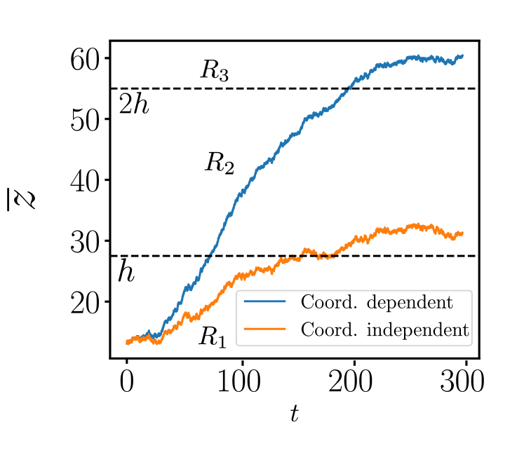
(a)

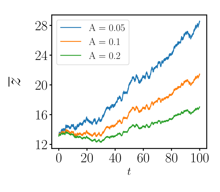
(b)

Figure 4: Time evolution of the center of mass of polymer chain, $\bar{z}$ (a) compared in the presence (case I) and absence (case II) of coordinate dependent damping (b) compared in the presence of coordinate dependent damping for various damping strengths as shown.

IV Discussion

It is counter-intuitive in the context of diffusion to think of diffusion creating concentration gradient. This is counter-intuitive in the sense of normal (uniform) diffusion processes, however, it turns out to be a general phenomenon in the presence of diffusion gradients when treated as an Itô-process. An Itô-process does not introduce correlations in the thermal noise and the thermal noise remains a white noise. Itô’s convention is essential to keep thermal noise correlation free and not coloured when diffusion is coordinate-dependent and the dynamics is an over-damped one. Any coloured noise in the oper-damped dynamics will break the thermal equilibrium of a Brownian particle which is supposed to be always in thermal equilibrium with the heat-bath at all the times. This is because, the limit of the Brownian particle’s relaxation time to equilibrium is taken to zero in the over-damped case.

Thus, the Itô-process in the presence of coordinate-dependent diffusion, which is quite ubiquitous, could potentially explain new physics which might have the clue to understand transport processes through constricted regions and apparent anti-diffusion. In living systems, such diffusion driven counter processes to the idea of normal diffusion might hold the key to generally understanding structural transitions as well. There could exist an effective attractive force driven by hydrodynamics near interfaces of particles, in general, in classical regime is a novel ingredient which has not been paid much attention to in the literature. This is where exists the need to explore such mesoscopic systems under Itô’s convention.

Appendix A : BASICS OF AN ITÔ PROCESS

Consider the following overdamped Langevin equation for the $i^{th}$ particle in presence of a force $\mathbf{F}_{i}$, Gaussian noise $\bm{\eta}_{i}(t)$ and coordinate-dependent damping $\Gamma_{i}$ in equilibrium with heat bath at temperature $T$:

$${}\frac{d{\mathbf{r}_{i}}}{dt} = \frac{\mathbf{F}_{i}}{\Gamma_{i}}+\sqrt{\frac{2k_{B}T}{\Gamma_{i}}}{\bm{\eta}}_{i}(t).$$

This equation is numerically evolved using the Euler-Maruyama scheme. In this paper, we solve this equation by considering it as an Itô process. The Itô process corresponds to utilizing a correlation-free (non-anticipating) noise. This means while numerically evolving the dynamics, at every time step ($\Delta t$) of evolution, the particle’s position at the start of the interval $\Delta t$ determines the damping/diffusivity. Thus when considered as an Itô process, the following Euler-Maruyama updation prescription is used:

$${}\mathbf{r}_{i}(t+\Delta t) =\mathbf{r}_{i}(t) +\frac{\mathbf{F}_{i}\{\mathbf{r}_{i}(t)\}}{\Gamma_{i}\{\mathbf{r}_{i}(t)\}}\Delta t+\sqrt{\frac{2k_{B}T\Delta t}{\Gamma_{i}\{\mathbf{r}_{i}(t)\}}}\bm{\mathcal{N}}(0,1),$$

Here $\Delta t$ is the discretized time step by which particle’s position is updated after each iteration. $\mathbf{F}_{i}\{\mathbf{r}_{i}(t)\}$ and $\Gamma_{i}\{\mathbf{r}_{i}(t)\}$ respectively denote the net force and damping coefficient of $i^{th}$ particle at time $t$. $\bm{\mathcal{N}}(0,1)$ is a three-dimensional Gaussian distributed random variable vector with zero mean, unit standard deviation, and zero cross-correlation.

We implement the following methodology for our simulations:

1. Initialise the system.

2. Evaluate the net force and damping associated with each particle.

3. Generate Gaussian distributed random variables with the above mentioned desirable properties and then update the position of each particle using the Itô process discretization prescription.

4. Go back to step (2) and repeat.

Appendix B : Diffusion diode

Initialization in the Diffusion diode section corresponds to assigning random positions to particles inside their respective regions ($R_{1}$ and $R_{3}$ for cases I and II, respectively) at the start of the simulation. In the simulations, new random seeds and different uncorrelated sequences of random numbers are used to generate Gaussian-distributed random variables. We run the simulation till a steady state is reached. Thermal energy $k_{B}T$ and distance parameter $r_{l}$ are our reference scales for energy and length in simulation.

We fix $k_{B}T=1$, $r_{l}=0.5$ and number of particles $N=100$, with repulsion strength parameter set to $\kappa=1000$. The box dimensions chosen are $l_{x}=14$, $l_{y}=l_{z}=5$. To model the damping profile, we chose $A=4.5$ and $x_{0}=\frac{1}{2}l_{x}=7$. We use discretized time step $\Delta t=5\times 10^{-4}$ to evolve equation $(3)$. We consider three different damping profile parameters, which corresponds to changing $\beta$ keeping other damping parameters $A$ and $x_{0}$ fixed. We simulate this for both cases (I and II). The choice of $\beta$ decides the width of $R_{2}$ in $x$ direction. The following values of $\beta$’s are chosen: 2.5, 3.3, and 5.0, corresponding to $R_{2}$’s widths (in $x$ direction) 4, 3, and 2 respectively. Each simulation is run for $10^{7}$ iterations with successive data recorded every $100$ iterations. We generate $100$ ensembles for each case for a fixed $\beta$ and perform an ensemble average to obtain quantities of interest. ${n}_{f}$ and ${n}_{b}$ are the quantities of interest here, obtained by averaging over 100 ensembles.

APPENDIX C : Entropic pulling of a chain

The polymer is initialized in an identical unfolded linear chain conformation (coincident on $z$ axis lying in $R_{1}$ at the start of the simulation) in all the ensembles for cases I and II. We generate $50$ ensembles for cases I and II. $k_{B}T$ and $r_{min}$ serve as fundamental energy and length benchmarks in our simulations. Both are normalized to unity, $k_{B}T=1$ and $r_{min}=1$. The polymer consists of $N=25$ monomers. The geometric parameters defining the funnel geometry are $\mathcal{R}=3$, $r=2$, $h=27.5$. Interaction parameters are set at $\alpha=100$, $\epsilon=1.5$, $\sigma=1.5$, $\kappa=1000$ and $A=0.05$. Discretised time step $\Delta t=10^{-6}$ is employed and the simulations is run for $3\times 10^{8}$ iterations with monomer positions recorded every $10^{3}$ iterations.
Now when we remove regions $R_{1}$ and $R_{3}$ and place the polymer chain in a geometry that only consists of $R_{2}$, we use following parameters: ${R}=3$, $r=2$, $h=200$, interaction parameters are set at $\alpha=100$, $\epsilon=1.5$, $\sigma=1.5$, $\kappa=1000$, and time step of $\Delta t=10^{-6}$ is employed. The damping is coordinate dependent, $\Gamma_{i}=\frac{A}{s_{i}(z_{i})}$, where $s_{i}(z_{i})=r+(h-z_{i})(\frac{\mathcal{R}-r}{h})$. The simulations is run for $10^{8}$ iterations with monomer positions recorded every $10^{3}$ iterations. We generate 200 ensembles for each value of $A$ and evaluate $\bar{z}$ .

References

- Purcell [1977] E. M. Purcell, Life at low reynolds number, American journal of physics 45, 3 (1977).
- Nachtigall [1981] W. Nachtigall, Hydromechanics and biology, Biophysics of structure and mechanism 8, 1 (1981).
- Cohen and Boyle [2010] N. Cohen and J. H. Boyle, Swimming at low reynolds number: a beginners guide to undulatory locomotion, Contemporary Physics 51, 103 (2010).
- Foster et al. [2018] D. A. Foster, R. Petrosyan, A. G. Pyo, A. Hoffmann, F. Wang, and M. T. Woodside, Probing position-dependent diffusion in folding reactions using single-molecule force spectroscopy, Biophysical journal 114, 1657 (2018).
- Neupane et al. [2017] K. Neupane, F. Wang, and M. Woodside, Direct measurement of sequence-dependent transition path times and conformational diffusion in dna duplex formation, Biophysical Journal 112, 471a (2017).
- Cellmer et al. [2008] T. Cellmer, E. R. Henry, J. Hofrichter, and W. A. Eaton, Measuring internal friction of an ultrafast-folding protein, Proceedings of the National Academy of Sciences 105, 18320 (2008).
- Faucheux and Libchaber [1994] L. P. Faucheux and A. J. Libchaber, Confined brownian motion, Physical Review E 49, 5158 (1994).
- Lin et al. [2000] B. Lin, J. Yu, and S. A. Rice, Direct measurements of constrained brownian motion of an isolated sphere between two walls, Physical review E 62, 3909 (2000).
- Noguchi et al. [2016] J. Noguchi, T. Hayama, S. Watanabe, H. Ucar, S. Yagishita, N. Takahashi, and H. Kasai, State-dependent diffusion of actin-depolymerizing factor/cofilin underlies the enlargement and shrinkage of dendritic spines, Scientific reports 6, 32897 (2016).
- Sharma et al. [2010] P. Sharma, S. Ghosh, and S. Bhattacharya, A high-precision study of hindered diffusion near a wall, Applied Physics Letters 97 (2010).
- Berezhkovskii and Makarov [2017] A. M. Berezhkovskii and D. E. Makarov, Communication: Coordinate-dependent diffusivity from single molecule trajectories, The Journal of chemical physics 147 (2017).
- Best and Hummer [2010] R. B. Best and G. Hummer, Coordinate-dependent diffusion in protein folding, Proceedings of the National Academy of Sciences 107, 1088 (2010).
- Oliveira et al. [2010] R. J. Oliveira, P. C. Whitford, J. Chahine, V. B. Leite, and J. Wang, Coordinate and time-dependent diffusion dynamics in protein folding, Methods 52, 91 (2010).
- Roussel and Roussel [2004] C. J. Roussel and M. R. Roussel, Reaction–diffusion models of development with state-dependent chemical diffusion coefficients, Progress in biophysics and molecular biology 86, 113 (2004).
- Chahine et al. [2007] J. Chahine, R. J. Oliveira, V. B. Leite, and J. Wang, Configuration-dependent diffusion can shift the kinetic transition state and barrier height of protein folding, Proceedings of the National Academy of Sciences 104, 14646 (2007).
- Bhattacharyay [2019] A. Bhattacharyay, Equilibrium of a brownian particle with coordinate dependent diffusivity and damping: Generalized boltzmann distribution, Physica A: Statistical Mechanics and its Applications 515, 665 (2019).
- Goloubinoff and De Los Rios [2007] P. Goloubinoff and P. De Los Rios, The mechanism of hsp70 chaperones:(entropic) pulling the models together, Trends in biochemical sciences 32, 372 (2007).
- Sousa and Lafer [2019] R. Sousa and E. M. Lafer, The physics of entropic pulling: a novel model for the hsp70 motor mechanism, International journal of molecular sciences 20, 2334 (2019).
- De Los Rios et al. [2006] P. De Los Rios, A. Ben-Zvi, O. Slutsky, A. Azem, and P. Goloubinoff, Hsp70 chaperones accelerate protein translocation and the unfolding of stable protein aggregates by entropic pulling, Proceedings of the National Academy of Sciences 103, 6166 (2006).
- Sousa and Lafer [2006] R. Sousa and E. M. Lafer, Keep the traffic moving: mechanism of the hsp70 motor, Traffic 7, 1596 (2006).
- Rohland et al. [2022] L. Rohland, R. Kityk, L. Smalinskaitė, and M. P. Mayer, Conformational dynamics of the hsp70 chaperone throughout key steps of its atpase cycle, Proceedings of the National Academy of Sciences 119, e2123238119 (2022).
- Tomkiewicz et al. [2007] D. Tomkiewicz, N. Nouwen, and A. J. Driessen, Pushing, pulling and trapping–modes of motor protein supported protein translocation, FEBS letters 581, 2820 (2007).
- De Los Rios and Goloubinoff [2016] P. De Los Rios and P. Goloubinoff, Hsp70 chaperones use atp to remodel native protein oligomers and stable aggregates by entropic pulling, Nature structural & molecular biology 23, 766 (2016).
- Ganesan and Theg [2019] I. Ganesan and S. M. Theg, Structural considerations of folded protein import through the chloroplast toc/tic translocons, Febs Letters 593, 565 (2019).
- Yu and Sukenik [2023] F. Yu and S. Sukenik, Structural preferences shape the entropic force of disordered protein ensembles, The Journal of Physical Chemistry B (2023).
- Hwang and Karplus [2019] W. Hwang and M. Karplus, Structural basis for power stroke vs. brownian ratchet mechanisms of motor proteins, Proceedings of the National Academy of Sciences 116, 19777 (2019).
- Craig [2018] E. A. Craig, Hsp70 at the membrane: driving protein translocation, BMC biology 16, 1 (2018).
- Roos [2014] N. Roos, Entropic forces in brownian motion, American Journal of Physics 82, 1161 (2014).
- Neumann [1980] R. M. Neumann, Entropic approach to brownian movement, American Journal of Physics 48, 354 (1980).
- Rukes et al. [2024] V. Rukes, M. E. Rebeaud, L. Perrin, P. De Los Rios, and C. Cao, Single-molecule evidence of entropic pulling by hsp70 chaperones, bioRxiv , 2024 (2024).
- Bhattacharyay [2023] A. Bhattacharyay, Equilibrium with coordinate dependent diffusion: Comparison of different stochastic processes, arXiv preprint arXiv:2309.06567 (2023).
- Bressloff [2014] P. C. Bressloff, Stochastic processes in cell biology, Vol. 41 (Springer, 2014).
- Allen [2010] L. J. Allen, An introduction to stochastic processes with applications to biology (CRC press, 2010).
- Phillips et al. [2012] R. Phillips, J. Kondev, J. Theriot, and H. Garcia, Physical biology of the cell (Garland Science, 2012).
- Alon [2019] U. Alon, An introduction to systems biology: design principles of biological circuits (Chapman and Hall/CRC, 2019).
- Peliti and Pigolotti [2021] L. Peliti and S. Pigolotti, Stochastic Thermodynamics: An Introduction (Princeton University Press, 2021).
- Sattin [2008] F. Sattin, Fick’s law and fokker–planck equation in inhomogeneous environments, Physics Letters A 372, 3941 (2008).
- Bengfort et al. [2016] M. Bengfort, H. Malchow, and F. M. Hilker, The fokker–planck law of diffusion and pattern formation in heterogeneous environments, Journal of mathematical biology 73, 683 (2016).
- Vázquez and Márkus [2010] F. Vázquez and F. Márkus, Non-fickian particle diffusion in confined plasmas and the transition from diffusive transport to density waves propagation, Physics of Plasmas 17 (2010).
- Van Milligen et al. [2005] B. P. Van Milligen, P. Bons, B. A. Carreras, and R. Sanchez, On the applicability of fick’s law to diffusion in inhomogeneous systems, European journal of physics 26, 913 (2005).
- Maniar and Bhattacharyay [2021] R. Maniar and A. Bhattacharyay, Random walk model for coordinate-dependent diffusion in a force field, Physica A: Statistical Mechanics and its Applications 584, 126348 (2021).
- Sharma and Bhattacharyay [2020] M. Sharma and A. Bhattacharyay, Conversion of heat to work: An efficient inchworm, Physica Scripta 95, 105004 (2020).
- Dhawan and Bhattacharyay [2024] A. Dhawan and A. Bhattacharyay, Itô–distribution from gibbs measure and a comparison with experiment, Physica A: Statistical Mechanics and its Applications , 129599 (2024).
- Bhattacharyay [2020] A. Bhattacharyay, Generalization of stokes–einstein relation to coordinate dependent damping and diffusivity: an apparent conflict, Journal of Physics A: Mathematical and Theoretical 53, 075002 (2020).
- Sharma and Bhattacharyay [2023] M. Sharma and A. Bhattacharyay, Spontaneous collective transport in a heat-bath, Physica A: Statistical Mechanics and its Applications 626, 129082 (2023).
- Bhattacharyay [2012] A. Bhattacharyay, Directed transport in equilibrium: A model study, Physica A: Statistical Mechanics and its Applications 391, 1111 (2012).