A Statistical Investigation of the Neupert Effect in Solar Flares Observed with ASO-S/HXI
Abstract
The Neupert effect refers to the strong correlation between the soft X-ray (SXR) light curve and the time-integrated hard X-rays (HXR) or microwave flux, which is frequently observed in solar flares. In this article, we therefore utilized the newly launched Hard X-ray Imager (HXI) on board the Advanced Space-based Solar Observatory to investigate the Neupert effect during solar flares. By checking the HXR light curves at 2050 keV, a sample of 149 events that cover the flare impulsive phase were selected. Then, we performed a cross-correlation analysis between the HXR fluence (i.e., the time integral of the HXR flux) and the SXR 18 Å flux measured by the Geostationary Operational Environmental Satellite. All the selected flares show high correlation coefficients (0.90), which seem to be independent of the flare location and class. The HXR fluences tend to increase linearly with the SXR peak fluxes. Our observations indicate that all the selected flares obey the Neupert effect.
keywords:
flares, Neupert effect, X-ray emission, radio emission1 Introduction
Neupert (1968) first noted that the shape of the soft X-ray (SXR) flux appeared to resemble the time-integrated microwave light curve during the impulsive phase of a solar flare. Such close relationship was also observed between the SXR light curve and the cumulative time integral of the hard X-ray (HXR) flux, this was dubbed as ‘Neupert effect’ (e.g. Hudson, 1991; Yu, Li, and Gan, 2020; Li et al., 2023c). The empirical correlation suggests that a causal relationship between the nonthermal and thermal emissions could exist in a solar flare. That is, the instantaneous radiation in the SXR waveband depends on the accumulated energy that is deposited by the electron beam during the flare impulsive phase (e.g. Neupert, 1968; Hudson, 1991). Based on the thick-target flare model, the HXR emission is produced by the nonthermal bremsstrahlung via Coulomb collisions, whereas the SXR emission is the cumulative energy produced by the thermal bremsstrahlung that is also related to the same electron beam. During this process, the heated plasma via the thermal bremsstrahlung could rapidly expand up into the upper atmosphere, called as ‘chromospheric evaporation’ (e.g. Fisher, Canfield, and McClymont, 1985; Battaglia, Fletcher, and Benz, 2009; Tian et al., 2015; Tian and Chen, 2018; Li, Ning, and Zhang, 2015; Li, Hong, and Ning, 2022). Therefore, the Neupert effect could be regarded as an evidence of the chromospheric evaporation driven by nonthermal electrons (e.g. Lee, Petrosian, and McTiernan, 1995; McTiernan, Fisher, and Li, 1999; Mann, Aurass, and Warmuth, 2006; Ning, 2009; Ning and Cao, 2010a; Li et al., 2023b).
The Neupert effect has been studied by many authors since it was reported by Neupert (1968). Some authors estimated the nonthermal and thermal energies using X-ray spectroscopic imager observations to study the Neupert effect in solar flares (e.g. Datlowe, Elcan, and Hudson, 1974; Starr et al., 1988; Feldman, 1990; Dennis et al., 2003; Ning, 2008b; Ning and Cao, 2010b). This is because the SXR radiation is related to the thermal energy accumulated in the solar corona, while the HXR emission is linked to the nonthermal energy during the solar flare. However, those observations had conflicting results. Dennis (1988) proposed that the causal correlation between SXR and HXR emissions could be attributed to different flare types or phases (see also Dennis and Zarro, 1993). The Neupert-type flare, which followed the Neupert effect, was usually found in the model that the flare energy was released primarily by nonthermal electrons (e.g. Brown, 1971; Ning, 2009). Based on a statistical investigation of the time difference between the SXR maximum and the end of the HXR emission in solar flares, Veronig et al. (2002a) concluded that the chromospheric evaporation driven by electron beams plays a major role in Neupert-type flares (see also Veronig et al., 2002b, 2005). The Neupert effect was also observed in microflare data from the Reuven Ramaty High Energy Solar Spectroscopic Imager (RHESSI) (e.g. Ning, 2008a).
The recently launched Hard X-ray Imager (HXI; Su et al., 2019; Zhang et al., 2019) on board the Advanced Space-based Solar Observatory (ASO-S; Gan et al., 2019, 2023; Huang et al., 2019) provides a good chance to study the relationship between the SXR light curve and the time-integrated HXR flux during the impulsive phase of solar flares. In this study, we statistically investigated the Neupert effect in solar flares, which were simultaneously measured by ASO-S/HXI and the Geostationary Operational Environmental Satellite (GOES; Loto’aniu et al., 2019). The microwave emission of some flares were measured by Chashan Broadband Solar millimeter spectrometer (CBS; Shang et al., 2022; Yan et al., 2023) and the Nobeyama Radio Polarimeters (NoRP), which were used to confirm the Neupert effect. The article is organized as follows: Section 2 introduces the observations and data analysis, Section 3 shows our primary results, Section 4 presents our discussion, and a brief summary is given in Section 5.
2 Observations and Data Analysis
2.1 Observations
HXI is one of three payloads aboard ASO-S. It provides flare observations in the HXR energy range of 15300 keV. The time cadence is 4 s in the regular mode, and it can be as high as 0.125 s in the flare mode. Two types of data products are provided by the HXI team, Level Q1 and Level 1. In our study, the full-disk light curves at the energy channel of 2050 keV are used. The light curve is the sum of three flux monitors (D92, D93, and D94), which are derived from the data production of Level Q1. The time cadence of this data is 4 s in the regular mode and becomes 2 s in the flare mode.
GOES is designed to continuously monitor the atmospheric conditions, space weather, and solar activity. The X-Ray Sensor (XRS) aboard GOES provides SXR light curves at 18 Å and 0.54 Å, which can be used for detecting solar flares (Loto’aniu et al., 2019). They have an uniform time cadence of 1 s. We also used the microwave flux measured by CBS and NoRP to confirm the causal relationship between the thermal and nonthermal emissions. CBS is a newly built solar radio spectrograph at the Chashan Solar Observatory (CSO). It is the first solar-dedicated radio spectrometer in the millimeter regime of 3540 GHz, which has a time cadence of 0.53 s (Shang et al., 2023; Yan et al., 2023). NoRP provides the solar radio flux at six frequencies, and it has a time cadence of 1 s.
2.2 Data Analysis
ASO-S/HXI has captured hundreds of solar flares since its first light in the HXR energy range, which gives us an opportunity to statistically study the HXR emission in solar flares. However, the HXI data can be affected when ASO-S crosses the South Atlantic Anomaly (SAA) and the radiation belt (RB), resulting in incomplete flare data. So, we first selected solar flares that were observed completely by HXI, namely, the flares that showed significant enhancements during their impulsive phases at HXI 2050 keV, as shown in Figures 1 and 2. The main reason for using HXI 2050 keV flux is to maintain a significant number of flare events. Moreover, the selected flares had to be recorded by GOES at 18 Å, because in this way we could study the flare thermal emission in SXR. We finally chose 149 flares from the one-year HXI observations, i.e. from 11 November 2022 to 11 November 2023 during the increasing period of of Cycle 25, as listed in Table LABEL:tab1. Here, there are mainly two data biases in our event selection: (1) the 149 flares were completely recorded by GOES; (2) HXI 2050 keV fluxes showed obviously flare radiation during the impulsive phase.
In order to investigate the Neupert effect, we compared the cause relationship between the HXR fluence () and SXR flux () during the flare impulsive phase, as expressed in previous articles (e.g. Lee, Petrosian, and McTiernan, 1995; Veronig et al., 2002a)
| (1) | |||
| (2) |
where and denote the HXR light curve and its background flux, which were observed by ASO-S/HXI at 2050 keV. and are the start and end time of the HXR light curve. The HXR fluence is defined as the time integral of the HXR light curve after removing its background emission during the impulsive phase of a solar flare. According to the theoretical expectation that the HXR emission ends and the SXR maximum occurs at almost the same time for the Neupert-type flare, the end time of the HXR light curve is regarded as the maximum time of the SXR flux.
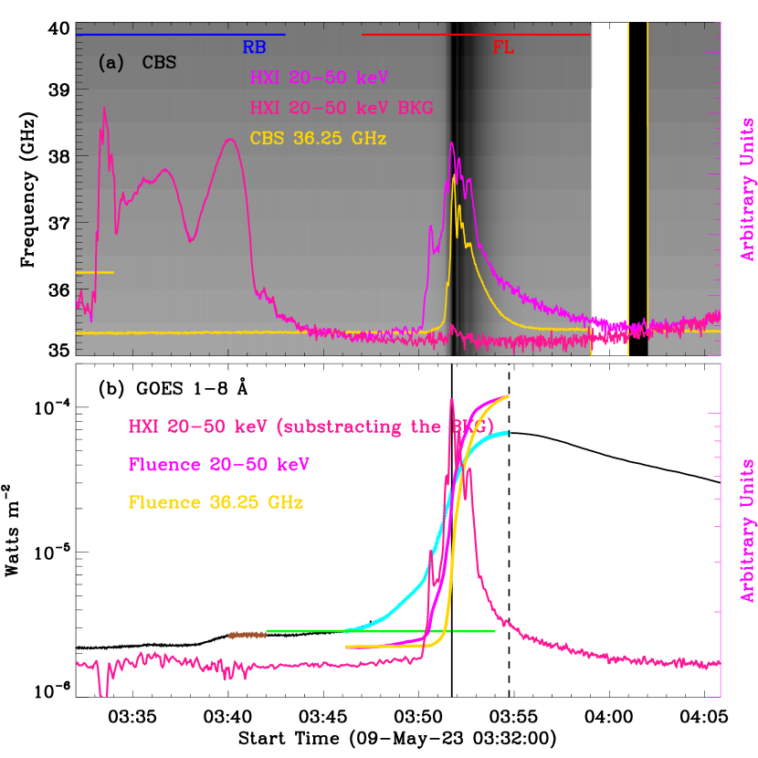
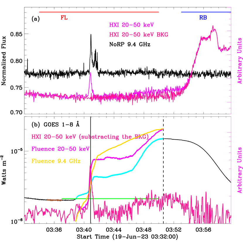
For a solar flare recorded by GOES, the start, peak, and stop time is automatically provided by the GOES team. In this study, we obtained these information from the Solar Flare Finder Widget, which is available via the Solar Software (Freeland and Handy, 1998; Milligan and Ireland, 2018). This widget also provides the flare locations, which are calculated from the Atmospheric Imaging Assembly images. Figure 1b presents the SXR flux recorded by GOES 18 Å, the horizontal green line outlines the duration of the impulsive phase; the start () and peak () time is extracted from the Solar Flare Finder Widget. The vertical lines mark the time when the HXR (solid) and SXR (dashed) emissions reach their maximum, respectively. Obviously, the SXR maximum time such as is different from given by the GOES team; is regarded as the end of the HXR emission. Similarly, is not equal to . In order to obtain , the SXR emission with a duration of two minutes before the solar flare () is first chosen as the background, as marked by the brown pluses. Then, a threshold is determined by the average value () plus a statistically significant (9 ) of the background emission, as shown by the green line. That is, occurs when the SXR flux exceeeds the threshold (). We want to state that and are identified from the SXR flux rather than the HXR light curve, because the HXR light curve measured by HXI has a high noise, especially for the non-flare flux. In such case, the fluctuation of the background is too large, and it is impossible to use a unique standard value. Figure 2b shows another flare recorded by GOES 18 Å; similar temporal properties confirm our selection.
3 Results
To show our statistical results, we first describe two events, as example.
3.1 Examples in the Sample List
Figure 1 shows an example of the solar flare that took place on 09 May 2023, which was an M6.5-class flare. Panel a draws the HXR light curves measured by HXI 2050 keV, the magenta and deep pink curves are the HXI data observed by three flux monitors and the corresponding background monitors, respectively. It can be immediately noticed that the radiation enhancement in the approximate period of 03:3303:44 UT is from the background rather than from the solar flare, since the magenta and deep pink curves overlap. This is mainly because ASO-S goes through the radiation belt (RB) during that time interval, as indicated by the blue line. On the other hand, the radiation enhancement between about 03:45 UT and 03:55 UT is the flare emission in the HXR channel and the background curve does not reveal any significant enhancement. The microwave flux in the frequency of 36.25 GHz (gold) further confirms that the radiation is from a solar flare. The background image is the radio dynamic spectrum in the frequency range of 3540 GHz observed by CBS, which clearly shows a group of microwave bursts accompanying the solar flare.
In Figure 1b, we show the SXR flux recorded by GOES at 18 Å, which starts at about 03:42 UT and peaks at around 03:54 UT111https://www.solarmonitor.org/?date=20230509, as outlined by the green line. We notice that both the SXR and HXR (deep pink curve) fluxes do not exhibit a significant enhancement at about 03:42 UT, which is not suitable for the start time () of the HXR fluence. Here, the time when the SXR flux exceeds the threshold () is regarded as , while the end time () of the HXR fluence is the time when the SXR flux reaches its maximum, based on the assumption that the SXR emission reaches its maximum when the HXR ends (Veronig et al., 2002a). Then, the HXR fluence can be calculated by integrating over the HXI flux after removing the background emission between the time interval and , as shown by the magenta curve. It matches well the SXR flux, as indicated by the cyan curve. Using the same method, the microwave fluence is estimated by integrating over the CBS flux from to , as shown by the gold curve. It seems to be a bit different from the SXR flux, which could be because the microwave flux starts later than the HXR flux, as shown by the magenta and gold line in Figure 1a.
Figure 2 presents another solar flare that occurred on 19 June 2023, which was an M1.4-class flare. The HXR light curves were observed by HXI 2050 keV, and the microwave flux was detected by NoRP 9.4 GHz. They both show a nonthermal pulse during the M1.4 flare, as shown in panel a. The SXR flux recorded by GOES 18 Å suggests that the flare starts at about 03:37 UT and peaks at around 03:50 UT222https://www.solarmonitor.org/?date=20230619. Similarly, these are not the HXR start and end times. Moreover, the SXR flux reveals two primary peaks during the flare impulsive phase, as shown in panel b. Using the same method, the HXR/micorwave fluence is estimated via integrating over the HXI and NoRP fluxes after subtracting their background from to , as indicated by the magenta and gold curves. Those two curves appear to match the SXR flux, particularly for the HXR fluence.
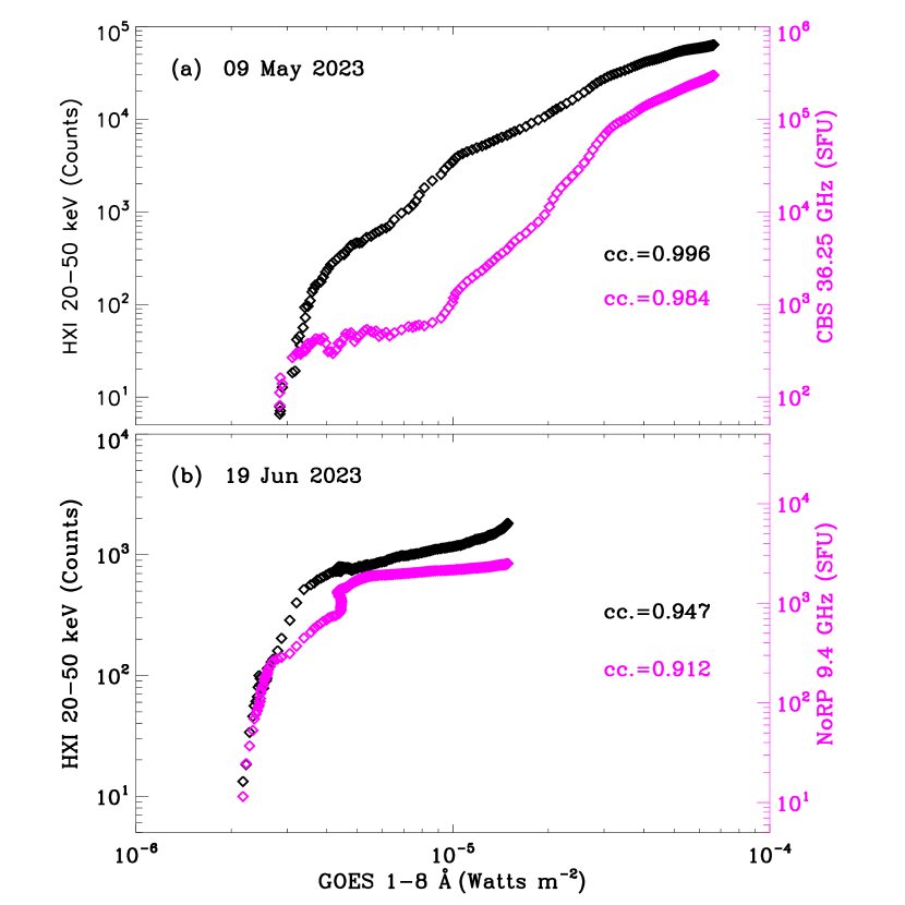
To look closely at their cause relationship, we perform a cross-correlation analysis between the SXR flux and the HXR and microwave fluences in the two flares, as shown in Figure 3. Here, the time cadences of the SXR and microwave light curves are both interpolated to the HXI time resolution, so they have the same points during the same time interval. A very high correlation coefficient (cc.) is obtained for the M6.5 flare on 09 May 2023, implying that it is completely consistent with the Neupert effect. Similarly to the observational result in Figure 1b, the correlation coefficient between the SXR flux and HXR fluence is higher than that between the SXR flux and microwave fluence. Conversely, the correlation coefficient for the M1.4 flare on 19 June 2023 is a little lower, which may suggest that it weakly agrees with the Neupert effect.
3.2 Statistical Results
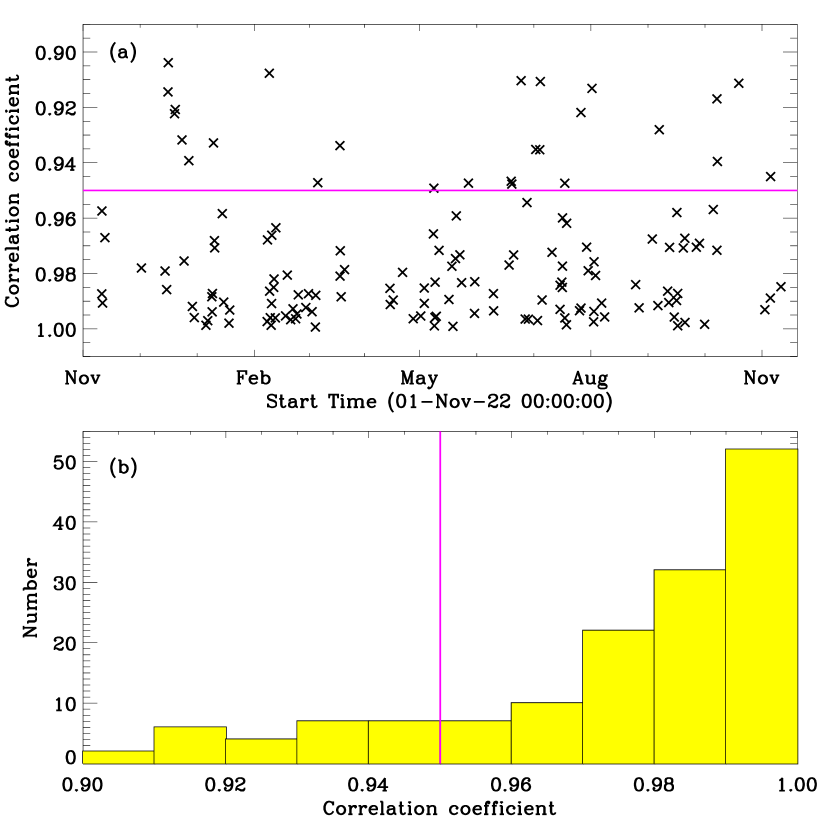
Based on the same method, we investigated the simple correlation between the HXR fluence and the SXR flux for 149 flares measured by ASO-S/HXI and GOES. Figure 4 presents the distribution of correlation coefficients, namely, the correlation coefficients as a function of time (panel a) and the histogram of the correlation coefficients (panel b). We can see that all these solar flares show high correlation coefficients, 0.90. Moreover, there are 123 flares that show correlation coefficients above 0.95, and only 26 flares below 0.95, as shown in the histogram of the correlation coefficients. That is, about 82.5% (123/149) of the studied flares show a strong correlation between the SXR flux and the time integral of the HXR emission. Here, a threshold of 0.95 (magenta line) is chosen, since it is a middle value for the correlation coefficients. We also considered the confidence interval at the level of 95% in wavelet analysis (e.g. Scargle, 1982; Torrence and Compo, 1998).
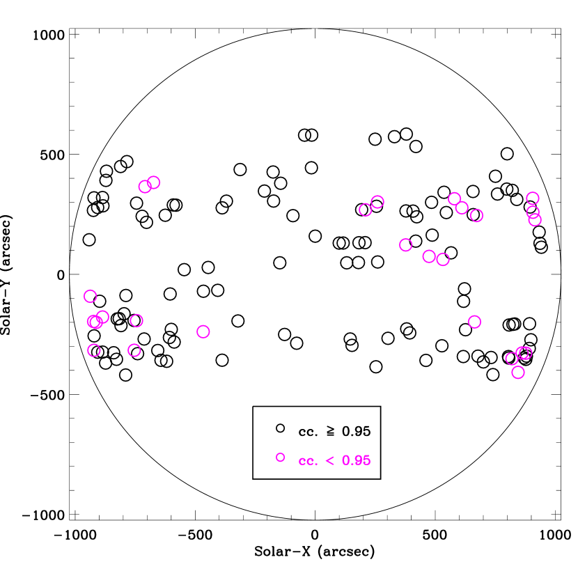
Figure 5 shows the locations of all these studied flares. The colors represent the different ranges of the correlation coefficients. As shown in Figure 5, these studied flares appear to be located at the low and middle latitude, including all the flares no matter if they have higher (0.95) or lower (0.95) correlation coefficients. On the other hand, these flares that show lower correlation coefficients seem to occur at the region that is close to the solar limb, east or west solar limbs. While those flares that have higher correlation coefficients appear in any low- and middle-latitude region, i.e. the solar limb and solar center.
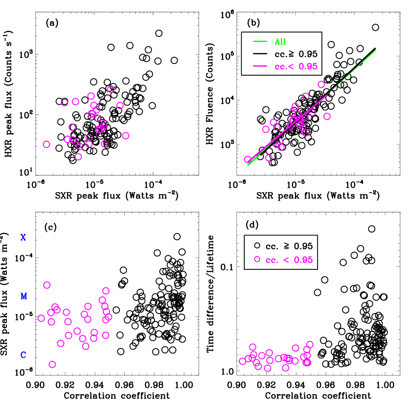
Figures 6 presents four scatter plots between some key parameters. Panels a and b show the HXR peak flux and fluence depending on the SXR peak flux. Comparing with the HXR peak flux, the HXR fluence exhibits a better linear relationship with the SXR peak flux, as indicated by the black line in panel b. Notice that the statistical result is based on all the selected flares, whether they have higher (cyan) or lower (magenta) correlation coefficients. The linear fitting is also performed for those flares that have higher and lower correlation coefficients, as indicated by the cyan and magenta lines, respectively. The two fitting results (black and magenta lines) are consistent with that for all the flares (green line), which may suggest that all these flares are obeying the Neupert effect. Figure 6c displays the SXR peak flux or GOES class depending on the correlation coefficient. It seems that these lower correlation coefficients tend to be related to small flares, while major flares tend to exhibit a higher correlation. However, we should state that this is mainly because the major flares are very rare in our study, i.e. only three X-class flares. Panel d presents the ratio between the time difference and lifetime depending on the correlation coefficient. Here, the time difference refers to the time delay between the HXR peak and the SXR maximum, as marked by the vertical solid and dashed lines in Figures 1b and 2b. The lifetime refers to the duration of the HXR fluence, i.e. . The lower correlation coefficients seem to appear in those flares that have a large ratio between the time difference and the lifetime. For instance, the ratio of those correlation coefficients below 0.95 is close to 1.0.
4 Discussion
In this study, 149 events were selected to investigate the causal relationship between the HXR fluence and the SXR flux, since the impulsive phases of these flares were completely observed by ASO-S/HXI in the energy range of 2050 keV. The SXR fluxes were recorded by GOES at 18 Å, and the HXR fluence was defined as the time integral of HXR light curves measured by HXI at 2050 keV. The microwave fluxes, which were measured by CBS and NoRP, were also used to examine the correlation between the microwave fluence and the SXR flux. For those selected solar flares, their HXR fluences were found to closely match the SXR fluxes, implying that the studied flares could follow the Neupert effect.
In this work, the causal correlation between the time integral of the HXR flux and the SXR emission is primarily identified as the correlation coefficient between the HXR fluence and the SXR flux during the flare impulsive phase. This is mainly because the HXR emission produced by the nonthermal electron is strongly related to the magnetic reconnection during the flare impulsive phase (e.g. Krucker et al., 2008; Shibata and Magara, 2011; Jiang et al., 2021; Li et al., 2023a). The duration of the time integral is determined from the SXR flux observed by GOES, since the HXR flux measured by ASO-S/HXI reveals a high noise level, which could increase the uncertainty in the start and end times. The start time () is regarded as the statistically significant excess of 9 above the background emission, similarly to the triggered mode of Konus-Wind333http://www.ioffe.ru/LEA/kwsun/. The end time () is defined as the maximum of the SXR flux, according to the fact that the maximum of SXR light curves and the end of HXR fluxes occur at nearly the same time (Veronig et al., 2002a). Then, the lifetime of the HXR fluence can be obtained as . We also estimated the time difference between the peak time of HXR pulse and the maximum time of the SXR flux. Noting that the time difference studied here is not the same as that reported by Veronig et al. (2002a), who investigated the time delay between the SXR maximum and the HXR end.
The correlation coefficients of all these 149 flares are greater than 0.90, which may suggest a close relationship between the HXR fluence and the SXR flux. The almost similar fitting results for these flares confirm the strong correlation. Moreover, about 82.5% of the studied flares show much higher correlation coefficients, 0.95. The statistical results agree with the standard flare model (e.g. Masuda et al., 1994; Su et al., 2013; Yan et al., 2018, 2022) or the CSHKP model (e.g. Carmichael, 1964; Sturrock, 1966; Hirayama, 1974; Kopp and Pneuman, 1976), indicating that the characterization we used in this study is reasonable. Twenty six flares show lower correlation coefficients, 0.95, but they are still larger than 0.90. All the lower correlation coefficients tend to show a large ratio between the time difference of the HXR peak and the SXR maximum and its lifetime (). For instance, their ratios could be as high as 1.0, indicating that the acceleration process of nonthermal electrons is much shorter than the heating process of thermal plasmas. Our observations suggest that those solar flares might have an additional heating process to the nonthermal electrons, which is consistent with the previous results (e.g. Veronig et al., 2002a; Li et al., 2021; Yu, Li, and Gan, 2020).
For all these 149 flares, the correlation coefficients seem to be independent on the flare location. They appear to take place in the middle- and low-latitude regions and not in the high-latitude region. While for these 26 flares that have lower correlation coefficients, they appear to be distributed close to the solar limb, i.e. the east and west limbs. The correlation coefficients do not exhibit a significant relation with the flare class or the SXR peak flux. The lower correlation coefficients seem to appear in small flares (C and M), which may because the intense flares (X) are very rare in our study, only three X-class flares. Similarly to pervious observations (cf. Veronig et al., 2002a), the HXR fluence displays a linear relationship with the SXR peak flux, suggesting that the flare energy released during the impulsive phase is primarily from the nonthermal electron beam (Priest and Forbes, 2002; Chen et al., 2017; Warmuth and Mann, 2016, 2020). Finally, we want to state that the HXI and GOES data are selected during the increasing period of Solar Cycle 25, which might motivate the curiosity to perform a similar study for the later time of the solar cycle.
5 Summary
Using the HXR and SXR light curves observed by ASO-S/HXI and GOES, we statistically investigated the Neupert effect during solar flares. Our primary results are summarized as follows:
(1) 149 flares are selected from the HXI database. These flares exhibit apparently radiation enhancements in the energy range of 2050 keV, and their impulsive phases are completely recorded by HXI.
(2) The selected flares show high correlation coefficients (0.90) between the HXR fluence and the SXR flux. 123 (82.5%) of them exhibit much higher correlation coefficients, 0.95.
(3) The HXR fluence displays a linear relationship with the SXR peak flux, and the correlation coefficient between the time integral of the HXR flux and the SXR light curve appears to be independent of the flare location and class. Our observational facts suggest that all the selected flares could follow the Neupert effect
This work is funded by the National Key R&D Program of China 2022YFF0503002 (2022YFF0503000), NSFC under grants 12073081, 12333010. D. Li is supported by Yunnan Key Laboratory of Solar Physics and Space Science under the number YNSPCC202207. This work is also supported by the Strategic Priority Research Program of the Chinese Academy of Sciences, Grant No. XDB0560000. ASO-S mission is supported by the Strategic Priority Research Program on Space Science, the Chinese Academy of Sciences, Grant No. XDA15320000.
ASO-S/HXI data: http://aso-s.pmo.ac.cn/sodc/dataArchive.jsp
GOES data: https://data.ngdc.noaa.gov/platforms/solar-space-observing-satellites/goes/
NoRP data: http://solar.nro.nao.ac.jp/norp/index.html
Z. J. Ning provided the idea, D. Li led this work and wrote the manuscript. H. Y. Dong participated in data analysis, W. Chen, Y. Su and Y. Huang participated the HXI data correction and some discussions. All authors reviewed the manuscript.
The authors declare that they have no conflicts of interest ..
References
- Battaglia, Fletcher, and Benz (2009) Battaglia, M., Fletcher, L., Benz, A.O.: 2009, Observations of conduction driven evaporation in the early rise phase of solar flares. A&A 498, 891. DOI. ADS.
- Brown (1971) Brown, J.C.: 1971, The Deduction of Energy Spectra of Non-Thermal Electrons in Flares from the Observed Dynamic Spectra of Hard X-Ray Bursts. Sol. Phys. 18, 489. DOI. ADS.
- Carmichael (1964) Carmichael, H.: 1964, A Process for Flares. In: NASA Special Publication 50, 451. ADS.
- Chen et al. (2017) Chen, Y., Wu, Z., Liu, W., Schwartz, R.A., Zhao, D., Wang, B., Du, G.: 2017, Double-coronal X-Ray and Microwave Sources Associated with a Magnetic Breakout Solar Eruption. ApJ 843, 8. DOI. ADS.
- Datlowe, Elcan, and Hudson (1974) Datlowe, D.W., Elcan, M.J., Hudson, H.S.: 1974, OSO-7 observations of solar x-rays in the energy range 10 100 keV. Sol. Phys. 39, 155. DOI. ADS.
- Dennis (1988) Dennis, B.R.: 1988, Solar Flare Hard X-Ray Observations. Sol. Phys. 118, 49. DOI. ADS.
- Dennis and Zarro (1993) Dennis, B.R., Zarro, D.M.: 1993, The Neupert Effect: what can it tell up about the Impulsive and Gradual Phases of Solar Flares. Sol. Phys. 146, 177. DOI. ADS.
- Dennis et al. (2003) Dennis, B.R., Veronig, A., Schwartz, R.A., Sui, L., Tolbert, A.K., Zarro, D.M., Rhessi Team: 2003, The neupert effect and new RHESSI measures of the total energy in electrons accelerated in solar flares. Advances in Space Research 32, 2459. DOI. ADS.
- Feldman (1990) Feldman, U.: 1990, The Beam-driven Chromospheric Evaporation Model of Solar Flares: A Model Not Supported by Observations from Nonimpulsive Large Flares. ApJ 364, 322. DOI. ADS.
- Fisher, Canfield, and McClymont (1985) Fisher, G.H., Canfield, R.C., McClymont, A.N.: 1985, Flare loop radiative hydrodynamics. V. Response to thick-target heating Dynamics of the thick-target heated chromosphere. ApJ 289, 414. DOI. ADS.
- Freeland and Handy (1998) Freeland, S.L., Handy, B.N.: 1998, Data Analysis with the SolarSoft System. Sol. Phys. 182, 497. DOI. ADS.
- Gan et al. (2019) Gan, W.-Q., Zhu, C., Deng, Y.-Y., Li, H., Su, Y., Zhang, H.-Y., Chen, B., Zhang, Z., Wu, J., Deng, L., Huang, Y., Yang, J.-F., Cui, J.-J., Chang, J., Wang, C., Wu, J., Yin, Z.-S., Chen, W., Fang, C., Yan, Y.-H., Lin, J., Xiong, W.-M., Chen, B., Bao, H.-C., Cao, C.-X., Bai, Y.-P., Wang, T., Chen, B.-L., Li, X.-Y., Zhang, Y., Feng, L., Su, J.-T., Li, Y., Chen, W., Li, Y.-P., Su, Y.-N., Wu, H.-Y., Gu, M., Huang, L., Tang, X.-J.: 2019, Advanced Space-based Solar Observatory (ASO-S): an overview. Research in Astronomy and Astrophysics 19, 156. DOI. ADS.
- Gan et al. (2023) Gan, W., Zhu, C., Deng, Y., Zhang, Z., Chen, B., Huang, Y., Deng, L., Wu, H., Zhang, H., Li, H., Su, Y., Su, J., Feng, L., Wu, J., Cui, J., Wang, C., Chang, J., Yin, Z., Xiong, W., Chen, B., Yang, J., Li, F., Lin, J., Hou, J., Bai, X., Chen, D., Zhang, Y., Hu, Y., Liang, Y., Wang, J., Song, K., Guo, Q., He, L., Zhang, G., Wang, P., Bao, H., Cao, C., Bai, Y., Chen, B., He, T., Li, X., Zhang, Y., Liao, X., Jiang, H., Li, Y., Su, Y., Lei, S., Chen, W., Li, Y., Zhao, J., Li, J., Ge, Y., Zou, Z., Hu, T., Su, M., Ji, H., Gu, M., Zheng, Y., Xu, D., Wang, X.: 2023, The Advanced Space-Based Solar Observatory (ASO-S). Sol. Phys. 298, 68. DOI. ADS.
- Hirayama (1974) Hirayama, T.: 1974, Theoretical Model of Flares and Prominences. I: Evaporating Flare Model. Sol. Phys. 34, 323. DOI. ADS.
- Huang et al. (2019) Huang, Y., Li, H., Gan, W.-Q., Li, Y.-P., Su, J.-T., Deng, Y.-Y., Feng, L., Su, Y., Chen, W., Lei, S.-J., Li, Y., Ge, Y.-Y., Su, Y.-N., Liu, S.-M., Zang, J.-J., Xu, Z.-L., Bai, X.-Y., Li, J.-W.: 2019, The Science Operations and Data Center (SODC) of the ASO-S mission. Research in Astronomy and Astrophysics 19, 164. DOI. ADS.
- Hudson (1991) Hudson, H.S.: 1991, Differential Emission-Measure Variations and the “Neupert Effect”. In: Bulletin of the American Astronomical Society 23, 1064. ADS.
- Jiang et al. (2021) Jiang, C., Feng, X., Liu, R., Yan, X., Hu, Q., Moore, R.L., Duan, A., Cui, J., Zuo, P., Wang, Y., Wei, F.: 2021, A fundamental mechanism of solar eruption initiation. Nature Astronomy 5, 1126. DOI. ADS.
- Kopp and Pneuman (1976) Kopp, R.A., Pneuman, G.W.: 1976, Magnetic reconnection in the corona and the loop prominence phenomenon. Sol. Phys. 50, 85. DOI. ADS.
- Krucker et al. (2008) Krucker, S., Battaglia, M., Cargill, P.J., Fletcher, L., Hudson, H.S., MacKinnon, A.L., Masuda, S., Sui, L., Tomczak, M., Veronig, A.L., Vlahos, L., White, S.M.: 2008, Hard X-ray emission from the solar corona. A&A Rev. 16, 155. DOI. ADS.
- Lee, Petrosian, and McTiernan (1995) Lee, T.T., Petrosian, V., McTiernan, J.M.: 1995, The Neupert Effect and the Chromospheric Evaporation Model for Solar Flares. ApJ 448, 915. DOI. ADS.
- Li, Hong, and Ning (2022) Li, D., Hong, Z., Ning, Z.: 2022, Simultaneous Observations of Chromospheric Evaporation and Condensation during a C-class Flare. ApJ 926, 23. DOI. ADS.
- Li, Ning, and Zhang (2015) Li, D., Ning, Z.J., Zhang, Q.M.: 2015, Observational Evidence of Electron-driven Evaporation in Two Solar Flares. ApJ 813, 59. DOI. ADS.
- Li et al. (2021) Li, D., Warmuth, A., Lu, L., Ning, Z.: 2021, An investigation of flare emissions at multiple wavelengths. Research in Astronomy and Astrophysics 21, 066. DOI. ADS.
- Li et al. (2023a) Li, D., Warmuth, A., Wang, J., Zhao, H., Lu, L., Zhang, Q., Dresing, N., Vainio, R., Palmroos, C., Paassilta, M., Fedeli, A., Dominique, M.: 2023a, Global Energetics of Solar Powerful Events on 2017 September 6. Research in Astronomy and Astrophysics 23, 095017. DOI. ADS.
- Li et al. (2023b) Li, D., Li, C., Qiu, Y., Rao, S., Warmuth, A., Schuller, F., Zhao, H., Shi, F., Xu, J., Ning, Z.: 2023b, Observational Signatures of Electron-driven Chromospheric Evaporation in a White-light Flare. ApJ 954, 7. DOI. ADS.
- Li et al. (2023c) Li, D., Hou, Z., Bai, X., Li, C., Fang, M., Zhao, H., Wang, J., Ning, Z.: 2023c, Simultaneous detection of flare-associated kink oscillations and extreme-ultraviolet waves. SCIENCE CHINA Technological Sciences. DOI. ADS.
- Loto’aniu et al. (2019) Loto’aniu, T.M., Redmon, R.J., Califf, S., Singer, H.J., Rowland, W., Macintyre, S., Chastain, C., Dence, R., Bailey, R., Shoemaker, E., Rich, F.J., Chu, D., Early, D., Kronenwetter, J., Todirita, M.: 2019, The GOES-16 Spacecraft Science Magnetometer. Space Sci. Rev. 215, 32. DOI. ADS.
- Mann, Aurass, and Warmuth (2006) Mann, G., Aurass, H., Warmuth, A.: 2006, Electron acceleration by the reconnection outflow shock during solar flares. A&A 454, 969. DOI. ADS.
- Masuda et al. (1994) Masuda, S., Kosugi, T., Hara, H., Tsuneta, S., Ogawara, Y.: 1994, A loop-top hard X-ray source in a compact solar flare as evidence for magnetic reconnection. Nature 371, 495. DOI. ADS.
- McTiernan, Fisher, and Li (1999) McTiernan, J.M., Fisher, G.H., Li, P.: 1999, The Solar Flare Soft X-Ray Differential Emission Measure and the Neupert Effect at Different Temperatures. ApJ 514, 472. DOI. ADS.
- Milligan and Ireland (2018) Milligan, R.O., Ireland, J.: 2018, On the Performance of Multi-Instrument Solar Flare Observations During Solar Cycle 24. Sol. Phys. 293, 18. DOI. ADS.
- Neupert (1968) Neupert, W.M.: 1968, Comparison of Solar X-Ray Line Emission with Microwave Emission during Flares. ApJ 153, L59. DOI. ADS.
- Ning (2008a) Ning, Z.: 2008a, RHESSI Microflares with Quiet Microwave Emission. ApJ 686, 674. DOI. ADS.
- Ning (2008b) Ning, Z.: 2008b, RHESSI Observations of the Neupert Effect in Three Solar Flares. Sol. Phys. 248, 99. DOI. ADS.
- Ning (2009) Ning, Z.: 2009, The investigation of the Neupert effect in two solar flares. Science in China: Physics, Mechanics and Astronomy 52, 1686. DOI. ADS.
- Ning and Cao (2010a) Ning, Z., Cao, W.: 2010a, Investigation of Chromospheric Evaporation in a Neupert-type Solar Flare. ApJ 717, 1232. DOI. ADS.
- Ning and Cao (2010b) Ning, Z., Cao, W.: 2010b, Investigation of the Neupert Effect in the Various Intervals of Solar Flares. Sol. Phys. 264, 329. DOI. ADS.
- Priest and Forbes (2002) Priest, E.R., Forbes, T.G.: 2002, The magnetic nature of solar flares. A&A Rev. 10, 313. DOI. ADS.
- Scargle (1982) Scargle, J.D.: 1982, Studies in astronomical time series analysis. II. Statistical aspects of spectral analysis of unevenly spaced data. ApJ 263, 835. DOI. ADS.
- Shang et al. (2022) Shang, Z., Xu, K., Liu, Y., Wu, Z., Lu, G., Zhang, Y., Zhang, L., Su, Y., Chen, Y., Yan, F.: 2022, A Broadband Solar Radio Dynamic Spectrometer Working in the Millimeter-wave Band. ApJS 258, 25. DOI. ADS.
- Shang et al. (2023) Shang, Z., Wu, Z., Liu, Y., Bai, Y., Lu, G., Zhang, Y., Zhang, L., Su, Y., Chen, Y., Yan, F.: 2023, The Calibration of the 35-40 GHz Solar Radio Spectrometer with the New Moon and a Noise Source. ApJS 268, 45. DOI. ADS.
- Shibata and Magara (2011) Shibata, K., Magara, T.: 2011, Solar Flares: Magnetohydrodynamic Processes. Living Reviews in Solar Physics 8, 6. DOI. ADS.
- Starr et al. (1988) Starr, R., Heindl, W.A., Crannell, C.J., Thomas, R.J., Batchelor, D.A., Magun, A.: 1988, Energetics and Dynamics of Simple Impulsive Solar Flares. ApJ 329, 967. DOI. ADS.
- Sturrock (1966) Sturrock, P.A.: 1966, Model of the High-Energy Phase of Solar Flares. Nature 211, 695. DOI. ADS.
- Su et al. (2013) Su, Y., Veronig, A.M., Holman, G.D., Dennis, B.R., Wang, T., Temmer, M., Gan, W.: 2013, Imaging coronal magnetic-field reconnection in a solar flare. Nature Physics 9, 489. DOI. ADS.
- Su et al. (2019) Su, Y., Liu, W., Li, Y.-P., Zhang, Z., Hurford, G.J., Chen, W., Huang, Y., Li, Z.-T., Jiang, X.-K., Wang, H.-X., Xia, F.-X.-Y., Chen, C.-X., Yu, W.-H., Yu, F., Wu, J., Gan, W.-Q.: 2019, Simulations and software development for the Hard X-ray Imager onboard ASO-S. Research in Astronomy and Astrophysics 19, 163. DOI. ADS.
- Tian and Chen (2018) Tian, H., Chen, N.-H.: 2018, Multi-episode Chromospheric Evaporation Observed in a Solar Flare. ApJ 856, 34. DOI. ADS.
- Tian et al. (2015) Tian, H., Young, P.R., Reeves, K.K., Chen, B., Liu, W., McKillop, S.: 2015, Temporal Evolution of Chromospheric Evaporation: Case Studies of the M1.1 Flare on 2014 September 6 and X1.6 Flare on 2014 September 10. ApJ 811, 139. DOI. ADS.
- Torrence and Compo (1998) Torrence, C., Compo, G.P.: 1998, A Practical Guide to Wavelet Analysis. Bulletin of the American Meteorological Society 79, 61. DOI. ADS.
- Veronig et al. (2002a) Veronig, A., Vršnak, B., Dennis, B.R., Temmer, M., Hanslmeier, A., Magdalenić, J.: 2002a, Investigation of the Neupert effect in solar flares. I. Statistical properties and the evaporation model. A&A 392, 699. DOI. ADS.
- Veronig et al. (2002b) Veronig, A., Vršnak, B., Temmer, M., Hanslmeier, A.: 2002b, Relative timing of solar flares observed at different wavelengths. Sol. Phys. 208, 297. DOI. ADS.
- Veronig et al. (2005) Veronig, A.M., Brown, J.C., Dennis, B.R., Schwartz, R.A., Sui, L., Tolbert, A.K.: 2005, Physics of the Neupert Effect: Estimates of the Effects of Source Energy, Mass Transport, and Geometry Using RHESSI and GOES Data. ApJ 621, 482. DOI. ADS.
- Warmuth and Mann (2016) Warmuth, A., Mann, G.: 2016, Constraints on energy release in solar flares from RHESSI and GOES X-ray observations. II. Energetics and energy partition. A&A 588, A116. DOI. ADS.
- Warmuth and Mann (2020) Warmuth, A., Mann, G.: 2020, Thermal-nonthermal energy partition in solar flares derived from X-ray, EUV, and bolometric observations. Discussion of recent studies. A&A 644, A172. DOI. ADS.
- Yan et al. (2023) Yan, F., Wu, Z., Shang, Z., Wang, B., Zhang, L., Chen, Y.: 2023, The First Flare Observation with a New Solar Microwave Spectrometer Working in 35-40 GHz. ApJ 942, L11. DOI. ADS.
- Yan et al. (2018) Yan, X.L., Yang, L.H., Xue, Z.K., Mei, Z.X., Kong, D.F., Wang, J.C., Li, Q.L.: 2018, Simultaneous Observation of a Flux Rope Eruption and Magnetic Reconnection during an X-class Solar Flare. ApJ 853, L18. DOI. ADS.
- Yan et al. (2022) Yan, X., Xue, Z., Jiang, C., Priest, E.R., Kliem, B., Yang, L., Wang, J., Kong, D., Song, Y., Feng, X., Liu, Z.: 2022, Fast plasmoid-mediated reconnection in a solar flare. Nature Communications 13, 640. DOI. ADS.
- Yu, Li, and Gan (2020) Yu, W.H., Li, Y.P., Gan, W.Q.: 2020, Statistical Studies on Modified Neupert Effect. Acta Astronomica Sinica 61, 53. ADS.
- Zhang et al. (2019) Zhang, Z., Chen, D.-Y., Wu, J., Chang, J., Hu, Y.-M., Su, Y., Zhang, Y., Wang, J.-P., Liang, Y.-M., Ma, T., Guo, J.-H., Cai, M.-S., Zhang, Y.-Q., Huang, Y.-Y., Peng, X.-Y., Tang, Z.-B., Zhao, X., Zhou, H.-H., Wang, L.-G., Song, J.-X., Ma, M., Xu, G.-Z., Yang, J.-F., Lu, D., He, Y.-H., Tao, J.-Y., Ma, X.-L., Lv, B.-G., Bai, Y.-P., Cao, C.-X., Huang, Y., Gan, W.-Q.: 2019, Hard X-ray Imager (HXI) onboard the ASO-S mission. Research in Astronomy and Astrophysics 19, 160. DOI. ADS.
| No. | Date | Time | Flux (GOES) | Fluence (HXI) | Position | cc. | |
| (W m-2) | (Counts) | ||||||
| 1 | 11 Nov 2022 | 01:31:14 UT | 01:35:59 UT | 4.8510-6 | 4.15103 | 100′′, 130′′ | 0.987 |
| 2 | 11 Nov 2022 | 03:15:28 UT | 03:17:16 UT | 2.5410-6 | 3.74103 | 116′′, 130′′ | 0.957 |
| 3 | 11 Nov 2022 | 11:33:13 UT | 11:40:41 UT | 1.2810-5 | 1.11104 | 182′′, 132′′ | 0.991 |
| 4 | 12 Nov 2022 | 18:01:55 UT | 18:03:53 UT | 6.9410-6 | 5.31103 | 419′′, 138′′ | 0.967 |
| 5 | 02 Dec 2022 | 09:15:20 UT | 09:20:54 UT | 8.6510-6 | 1.86103 | -924′′, 266′′ | 0.978 |
| 6 | 15 Dec 2022 | 01:29:03 UT | 01:37:33 UT | 1.6710-5 | 1.94103 | 678′′, -341′′ | 0.979 |
| 7 | 15 Dec 2022 | 22:23:52 UT | 22:40:16 UT | 5.8410-5 | 2.24104 | 805′′, -342′′ | 0.986 |
| 8 | 16 Dec 2022 | 15:35:11 UT | 15:41:00 UT | 1.3010-5 | 2.47103 | 862′′, -328′′ | 0.914 |
| 9 | 16 Dec 2022 | 19:04:49 UT | 19:11:14 UT | 9.3510-6 | 3.53103 | 877′′, -329′′ | 0.904 |
| 10 | 20 Dec 2022 | 04:09:19 UT | 04:10:17 UT | 4.7710-6 | 2.50103 | -709′′, 365′′ | 0.922 |
| 11 | 20 Dec 2022 | 13:52:46 UT | 14:06:49 UT | 1.1810-5 | 3.81103 | -674′′, 383′′ | 0.921 |
| 12 | 24 Dec 2022 | 04:09:41 UT | 04:14:16 UT | 4.2110-6 | 3.15103 | 259′′, 302′′ | 0.932 |
| 13 | 25 Dec 2022 | 06:56:45 UT | 07:00:59 UT | 8.3210-6 | 3.70103 | 485′′, 300′′ | 0.975 |
| 14 | 27 Dec 2022 | 20:35:16 UT | 20:37:21 UT | 4.2810-6 | 1.10103 | -922′′, -317′′ | 0.940 |
| 15 | 29 Dec 2022 | 18:15:04 UT | 18:20:37 UT | 2.2310-5 | 1.14104 | -922′′, 319′′ | 0.992 |
| 16 | 30 Dec 2022 | 19:08:04 UT | 19:09:43 UT | 4.5310-6 | 1.51103 | -144′′, 379′′ | 0.996 |
| 17 | 06 Jan 2023 | 00:47:58 UT | 00:57:40 UT | 1.2510-4 | 1.48105 | -906′′, -324′′ | 0.999 |
| 18 | 07 Jan 2023 | 00:44:25 UT | 00:52:07 UT | 1.6610-5 | 6.38103 | -840′′, -327′′ | 0.997 |
| 19 | 09 Jan 2023 | 04:49:50 UT | 04:51:18 UT | 5.0210-6 | 5.56102 | -921′′, -256′′ | 0.988 |
| 20 | 09 Jan 2023 | 08:46:30 UT | 09:01:18 UT | 2.1610-5 | 3.74103 | 381′′, -227′′ | 0.994 |
| 21 | 09 Jan 2023 | 13:17:47 UT | 13:22:14 UT | 1.0410-5 | 3.70103 | 394′′, -244′′ | 0.987 |
| 22 | 10 Jan 2023 | 02:13:06 UT | 02:16:18 UT | 1.0910-5 | 4.86103 | -886′′, -178′′ | 0.932 |
| 23 | 10 Jan 2023 | 14:45:51 UT | 14:47:36 UT | 9.2310-6 | 1.06103 | -825′′, -186′′ | 0.968 |
| 24 | 10 Jan 2023 | 17:47:35 UT | 17:48:31 UT | 1.3410-5 | 2.01103 | -816′′, -185′′ | 0.971 |
| 25 | 14 Jan 2023 | 20:08:31 UT | 20:21:22 UT | 3.6210-5 | 3.11104 | 626′′, -231′′ | 0.958 |
| 26 | 15 Jan 2023 | 14:20:12 UT | 14:31:34 UT | 4.9210-5 | 3.12104 | -809′′, -214′′ | 0.990 |
| 27 | 18 Jan 2023 | 10:28:35 UT | 10:34:58 UT | 1.8310-5 | 8.42103 | -322′′, -194′′ | 0.998 |
| 28 | 18 Jan 2023 | 20:44:36 UT | 20:47:23 UT | 9.7310-6 | 1.94103 | -212′′, 347′′ | 0.993 |
| 29 | 07 Feb 2023 | 23:05:24 UT | 23:07:36 UT | 6.6910-5 | 2.21104 | -44′′, 580′′ | 0.997 |
| 30 | 08 Feb 2023 | 02:48:26 UT | 02:53:40 UT | 2.1310-5 | 3.93103 | -15′′, 580′′ | 0.968 |
| 31 | 09 Feb 2023 | 02:49:43 UT | 03:10:37 UT | 3.4210-5 | 4.31103 | -937′′, -91′′ | 0.908 |
| 32 | 09 Feb 2023 | 07:15:59 UT | 07:17:59 UT | 1.2810-5 | 9.43102 | -898′′, -112′′ | 0.986 |
| 33 | 09 Feb 2023 | 14:50:47 UT | 14:56:46 UT | 1.5310-5 | 2.65103 | 250′′, 563′′ | 0.996 |
| 34 | 10 Feb 2023 | 02:49:51 UT | 03:03:55 UT | 3.7410-5 | 2.91104 | 330′′, 573′′ | 0.998 |
| 35 | 10 Feb 2023 | 08:03:34 UT | 08:05:44 UT | 1.6410-5 | 1.43103 | 379′′, 584′′ | 0.991 |
| 36 | 10 Feb 2023 | 10:47:02 UT | 10:49:21 UT | 9.7210-6 | 1.13103 | -788′′, -88′′ | 0.966 |
| 37 | 11 Feb 2023 | 11:31:47 UT | 11:34:36 UT | 1.5210-5 | 1.99103 | 800′′, 502′′ | 0.985 |
| 38 | 11 Feb 2023 | 15:44:14 UT | 15:48:45 UT | 1.2110-4 | 7.27104 | -604′′, -82′′ | 0.982 |
| 39 | 12 Feb 2023 | 08:39:05 UT | 08:48:04 UT | 3.3710-5 | 1.55104 | -466′′, -70′′ | 0.996 |
| 40 | 12 Feb 2023 | 15:35:20 UT | 15:37:57 UT | 1.1110-5 | 2.21103 | -406′′, -67′′ | 0.963 |
| 41 | 17 Feb 2023 | 19:46:53 UT | 20:16:54 UT | 2.2910-4 | 4.46105 | -811′′, 449′′ | 0.995 |
| 42 | 18 Feb 2023 | 18:33:17 UT | 18:35:52 UT | 7.3110-6 | 2.15103 | 423′′, 239′′ | 0.981 |
| 43 | 20 Feb 2023 | 14:54:29 UT | 14:58:15 UT | 4.5110-5 | 1.93104 | -870′′, 429′′ | 0.997 |
| 44 | 21 Feb 2023 | 20:04:26 UT | 20:16:59 UT | 5.1210-5 | 3.49104 | -785′′, 469′′ | 0.993 |
| 45 | 23 Feb 2023 | 06:12:32 UT | 06:13:55 UT | 1.6810-5 | 4.06103 | -313′′, 437′′ | 0.996 |
| 46 | 23 Feb 2023 | 23:11:18 UT | 23:13:38 UT | 6.8510-6 | 1.13103 | -176′′, 426′′ | 0.995 |
| 47 | 24 Feb 2023 | 17:13:04 UT | 17:15:41 UT | 1.2310-5 | 5.63103 | -16′′, 444′′ | 0.988 |
| 48 | 28 Feb 2023 | 17:38:57 UT | 17:50:28 UT | 8.6610-5 | 7.54104 | 420′′, 532′′ | 0.992 |
| 49 | 02 Mar 2023 | 04:42:49 UT | 04:50:17 UT | 9.3810-6 | 5.87103 | 751′′, 409′′ | 0.987 |
| 50 | 04 Mar 2023 | 02:24:15 UT | 02:25:56 UT | 5.9910-6 | 8.69102 | -703′′, 217′′ | 0.994 |
| 51 | 05 Mar 2023 | 21:30:19 UT | 21:35:47 UT | 5.1910-5 | 3.84104 | 798′′, 355′′ | 0.999 |
| 52 | 06 Mar 2023 | 02:11:46 UT | 02:28:13 UT | 5.8610-5 | 3.96104 | 821′′, 350′′ | 0.988 |
| 53 | 07 Mar 2023 | 04:00:29 UT | 04:05:01 UT | 4.7910-6 | 9.94102 | 906′′, 317′′ | 0.947 |
| 54 | 19 Mar 2023 | 02:14:36 UT | 02:15:42 UT | 3.1210-6 | 2.20103 | -754′′, -316′′ | 0.933 |
| 55 | 19 Mar 2023 | 03:55:16 UT | 03:56:38 UT | 2.5110-6 | 5.32102 | -740′′, -331′′ | 0.981 |
| 56 | 19 Mar 2023 | 06:31:30 UT | 06:35:31 UT | 4.6210-6 | 1.96103 | -740′′, -331′′ | 0.972 |
| 57 | 19 Mar 2023 | 18:05:44 UT | 18:08:48 UT | 5.1210-6 | 4.64103 | -656′′, -317′′ | 0.988 |
| 58 | 21 Mar 2023 | 13:51:33 UT | 13:53:57 UT | 5.5610-6 | 1.63103 | -619′′, -362′′ | 0.979 |
| 59 | 14 Apr 2023 | 23:22:59 UT | 23:27:51 UT | 1.6410-5 | 2.13103 | -721′′, 242′′ | 0.985 |
| 60 | 15 Apr 2023 | 03:02:56 UT | 03:03:26 UT | 4.0110-6 | 3.88102 | 618′′, -112′′ | 0.991 |
| 61 | 16 Apr 2023 | 17:33:40 UT | 17:43:46 UT | 9.1510-6 | 4.84103 | -872′′, 391′′ | 0.990 |
| 62 | 21 Apr 2023 | 17:48:07 UT | 18:11:44 UT | 1.7910-5 | 7.63103 | 153′′, -296′′ | 0.980 |
| 63 | 27 Apr 2023 | 11:11:22 UT | 11:13:53 UT | 2.1810-5 | 3.81103 | -77′′, -287′′ | 0.996 |
| 64 | 01 May 2023 | 13:05:45 UT | 13:09:25 UT | 7.7210-5 | 3.44104 | 617′′, -343′′ | 0.995 |
| 65 | 03 May 2023 | 10:07:31 UT | 10:14:16 UT | 3.1910-5 | 7.05103 | -625′′, 246′′ | 0.985 |
| 66 | 03 May 2023 | 10:39:40 UT | 10:45:20 UT | 7.5410-5 | 1.71104 | -625′′, 246′′ | 0.991 |
| 67 | 08 May 2023 | 08:22:43 UT | 08:25:48 UT | 3.1310-6 | 6.09103 | 193′′, 269′′ | 0.966 |
| 68 | 08 May 2023 | 14:16:48 UT | 14:21:03 UT | 9.8510-6 | 7.24103 | 209′′, 268′′ | 0.949 |
| 69 | 08 May 2023 | 20:16:11 UT | 20:25:19 UT | 2.3310-5 | 1.35104 | 255′′, 283′′ | 0.999 |
| 70 | 09 May 2023 | 03:46:10 UT | 03:54:44 UT | 6.6510-5 | 6.37104 | 407′′, 263′′ | 0.996 |
| 71 | 09 May 2023 | 06:07:42 UT | 06:13:32 UT | 1.2710-5 | 3.33103 | 378′′, 264′′ | 0.983 |
| 72 | 09 May 2023 | 20:34:22 UT | 20:52:38 UT | 5.0310-5 | 2.98104 | 546′′, 257′′ | 0.995 |
| 73 | 11 May 2023 | 08:51:30 UT | 09:01:38 UT | 2.2110-5 | 8.98103 | 622′′, -60′′ | 0.972 |
| 74 | 16 May 2023 | 16:34:19 UT | 16:43:26 UT | 9.6810-5 | 2.87104 | -873′′, -370′′ | 0.989 |
| 75 | 18 May 2023 | 06:15:26 UT | 06:26:14 UT | 1.0310-5 | 2.03103 | -906′′, 278′′ | 0.977 |
| 76 | 18 May 2023 | 20:17:07 UT | 20:23:36 UT | 4.0410-5 | 1.40104 | -884′′, 285′′ | 0.999 |
| 77 | 20 May 2023 | 04:41:04 UT | 04:50:06 UT | 7.0310-6 | 2.66103 | -790′′, -419′′ | 0.975 |
| 78 | 20 May 2023 | 14:56:09 UT | 14:59:48 UT | 6.1610-5 | 1.01104 | -744′′, 297′′ | 0.959 |
| 79 | 22 May 2023 | 13:26:08 UT | 13:27:28 UT | 7.6610-6 | 2.39103 | -370′′, 305′′ | 0.973 |
| 80 | 23 May 2023 | 12:08:52 UT | 12:13:53 UT | 3.9910-5 | 7.37103 | -174′′, 305′′ | 0.983 |
| 81 | 27 May 2023 | 04:33:28 UT | 04:35:42 UT | 8.8010-6 | 5.01103 | 611′′, 277′′ | 0.947 |
| 82 | 30 May 2023 | 10:17:38 UT | 10:21:58 UT | 1.4110-5 | 9.11103 | 877′′, -354′′ | 0.994 |
| 83 | 30 May 2023 | 13:36:55 UT | 13:38:53 UT | 1.6610-5 | 6.25103 | 528′′, -298′′ | 0.983 |
| 84 | 09 Jun 2023 | 14:31:54 UT | 14:40:00 UT | 4.6110-6 | 1.27103 | -128′′, -250′′ | 0.987 |
| 85 | 09 Jun 2023 | 16:52:22 UT | 17:11:26 UT | 2.5110-5 | 1.37104 | -642′′, -358′′ | 0.993 |
| 86 | 18 Jun 2023 | 00:28:06 UT | 00:31:37 UT | 1.3710-5 | 9.98103 | -388′′, -358′′ | 0.977 |
| 87 | 19 Jun 2023 | 03:38:54 UT | 03:50:37 UT | 1.4910-5 | 1.82103 | -923′′, -197′′ | 0.947 |
| 88 | 19 Jun 2023 | 12:08:12 UT | 12:14:18 UT | 1.2110-5 | 2.73103 | -912′′, -200′′ | 0.948 |
| 89 | 20 Jun 2023 | 10:49:23 UT | 11:06:05 UT | 8.7410-6 | 2.65103 | 806′′, -349′′ | 0.973 |
| 90 | 24 Jun 2023 | 12:13:23 UT | 12:17:03 UT | 1.1710-5 | 2.93103 | 580′′, 315′′ | 0.910 |
| 91 | 26 Jun 2023 | 16:13:09 UT | 16:22:22 UT | 1.6510-5 | 3.04103 | 536′′, 342′′ | 0.996 |
| 92 | 27 Jun 2023 | 15:01:32 UT | 15:14:25 UT | 1.2910-5 | 1.63103 | 657′′, 345′′ | 0.954 |
| 93 | 28 Jun 2023 | 08:32:00 UT | 08:44:47 UT | 1.9910-5 | 6.26103 | 759′′, 335′′ | 0.997 |
| 94 | 02 Jul 2023 | 08:47:59 UT | 08:52:50 UT | 8.9610-6 | 3.39103 | 672′′, 245′′ | 0.935 |
| 95 | 03 Jul 2023 | 06:47:15 UT | 06:53:14 UT | 1.4010-5 | 4.65103 | -588′′, -282′′ | 0.997 |
| 96 | 04 Jul 2023 | 12:23:54 UT | 12:35:53 UT | 1.4910-5 | 1.23104 | 907′′, 259′′ | 0.935 |
| 97 | 04 Jul 2023 | 19:11:32 UT | 19:27:51 UT | 8.1210-6 | 2.45103 | 915′′, 227′′ | 0.911 |
| 98 | 05 Jul 2023 | 18:14:26 UT | 18:17:05 UT | 4.4510-6 | 1.88103 | -886′′, -324′′ | 0.990 |
| 99 | 11 Jul 2023 | 02:11:18 UT | 02:14:13 UT | 8.9010-6 | 2.11103 | -886′′, 320′′ | 0.972 |
| 100 | 15 Jul 2023 | 09:49:43 UT | 09:53:15 UT | 1.0910-5 | 3.84103 | -591′′, 289′′ | 0.993 |
| 101 | 15 Jul 2023 | 10:07:25 UT | 10:09:53 UT | 2.3510-5 | 8.88103 | -580′′, 288′′ | 0.984 |
| 102 | 16 Jul 2023 | 08:33:14 UT | 08:40:48 UT | 5.0510-6 | 2.46103 | 732′′, -346′′ | 0.983 |
| 103 | 16 Jul 2023 | 15:06:32 UT | 15:09:02 UT | 1.9210-5 | 1.43104 | -388′′, 277′′ | 0.985 |
| 104 | 16 Jul 2023 | 17:12:35 UT | 17:19:24 UT | 5.9010-6 | 2.99103 | 700′′, -365′′ | 0.977 |
| 105 | 16 Jul 2023 | 17:38:41 UT | 17:48:13 UT | 4.0410-5 | 1.82105 | 740′′, -418′′ | 0.960 |
| 106 | 17 Jul 2023 | 22:44:44 UT | 22:55:20 UT | 2.7410-5 | 2.28104 | 845′′, -408′′ | 0.947 |
| 107 | 17 Jul 2023 | 23:19:24 UT | 23:34:30 UT | 5.0210-5 | 6.45104 | 870′′, -348′′ | 0.996 |
| 108 | 18 Jul 2023 | 20:19:40 UT | 20:28:07 UT | 2.1610-5 | 7.20103 | 880′′, -341′′ | 0.999 |
| 109 | 18 Jul 2023 | 22:40:54 UT | 22:44:12 UT | 8.7410-6 | 2.48103 | 892′′, -309′′ | 0.962 |
| 110 | 25 Jul 2023 | 21:11:37 UT | 21:16:47 UT | 1.6710-5 | 3.99103 | -600′′, -229′′ | 0.993 |
| 111 | 26 Jul 2023 | 15:18:53 UT | 15:24:03 UT | 8.1710-6 | 2.61103 | -467′′, -239′′ | 0.922 |
| 112 | 26 Jul 2023 | 15:53:19 UT | 15:59:41 UT | 2.0810-5 | 7.36103 | 840′′, 312′′ | 0.993 |
| 113 | 29 Jul 2023 | 16:16:11 UT | 16:24:14 UT | 1.4510-5 | 8.42103 | 146′′, -269′′ | 0.970 |
| 114 | 30 Jul 2023 | 13:12:59 UT | 13:15:51 UT | 4.4010-6 | 1.25103 | 303′′, -267′′ | 0.979 |
| 115 | 01 Aug 2023 | 14:03:30 UT | 14:09:16 UT | 1.4510-5 | 3.98103 | 664′′, -198′′ | 0.913 |
| 116 | 02 Aug 2023 | 10:47:22 UT | 10:49:48 UT | 1.3810-5 | 2.84103 | 808′′, -211′′ | 0.997 |
| 117 | 02 Aug 2023 | 14:50:28 UT | 14:52:27 UT | 1.7710-5 | 9.21103 | 823′′, -208′′ | 0.994 |
| 118 | 02 Aug 2023 | 16:20:12 UT | 16:22:19 UT | 1.4010-5 | 3.68103 | 831′′, -207′′ | 0.976 |
| 119 | 03 Aug 2023 | 11:49:19 UT | 11:55:10 UT | 2.1610-5 | 1.02104 | 893′′, -206′′ | 0.981 |
| 120 | 06 Aug 2023 | 18:25:18 UT | 18:40:32 UT | 5.5310-5 | 1.04105 | 936′′, 129′′ | 0.991 |
| 121 | 08 Aug 2023 | 09:25:10 UT | 09:31:16 UT | 3.7010-5 | 1.12104 | 895′′, 280′′ | 0.996 |
| 122 | 25 Aug 2023 | 01:00:29 UT | 01:09:15 UT | 1.4910-5 | 5.52103 | -713′′, -269′′ | 0.984 |
| 123 | 26 Aug 2023 | 21:47:48 UT | 21:50:20 UT | 2.6910-6 | 3.42103 | 942′′, 113′′ | 0.992 |
| 124 | 03 Sep 2023 | 00:15:25 UT | 00:23:00 UT | 1.1410-5 | 8.50103 | 933′′, 176′′ | 0.968 |
| 125 | 06 Sep 2023 | 00:48:50 UT | 00:50:29 UT | 5.2310-6 | 1.63103 | 208′′, 132′′ | 0.992 |
| 126 | 06 Sep 2023 | 17:54:58 UT | 17:56:29 UT | 5.6610-6 | 8.65102 | 377′′, 122′′ | 0.928 |
| 127 | 11 Sep 2023 | 06:00:03 UT | 06:01:16 UT | 1.0710-5 | 6.62102 | -796′′, -164′′ | 0.986 |
| 128 | 11 Sep 2023 | 21:09:46 UT | 21:14:02 UT | 8.3710-6 | 1.88103 | -93′′, 244′′ | 0.990 |
| 129 | 12 Sep 2023 | 06:49:39 UT | 07:02:15 UT | 2.5810-5 | 1.18104 | 487′′, 163′′ | 0.971 |
| 130 | 14 Sep 2023 | 19:28:21 UT | 19:31:52 UT | 2.0510-5 | 6.18103 | -148′′, 48′′ | 0.996 |
| 131 | 16 Sep 2023 | 00:45:53 UT | 00:49:49 UT | 2.9910-5 | 8.01103 | 131′′, 48′′ | 0.990 |
| 132 | 16 Sep 2023 | 05:28:22 UT | 05:38:45 UT | 3.4510-5 | 2.89104 | 180′′, 49′′ | 0.958 |
| 133 | 16 Sep 2023 | 15:50:13 UT | 15:51:00 UT | 2.7210-6 | 7.38102 | -942′′, 144′′ | 0.987 |
| 134 | 16 Sep 2023 | 15:55:40 UT | 15:56:57 UT | 4.1310-6 | 5.45102 | 260′′, 52′′ | 0.999 |
| 135 | 19 Sep 2023 | 15:41:42 UT | 15:52:32 UT | 4.3210-6 | 3.92102 | 658′′, 249′′ | 0.971 |
| 136 | 20 Sep 2023 | 12:10:33 UT | 12:12:49 UT | 3.5710-6 | 7.02102 | -446′′, 29′′ | 0.967 |
| 137 | 20 Sep 2023 | 14:14:12 UT | 14:19:06 UT | 8.3110-5 | 1.33105 | -546′′, 20′′ | 0.998 |
| 138 | 26 Sep 2023 | 16:16:37 UT | 16:18:08 UT | 4.5410-6 | 1.42103 | 253′′, -385′′ | 0.971 |
| 139 | 28 Sep 2023 | 09:05:38 UT | 09:07:30 UT | 1.3310-5 | 5.21103 | -828′′, -354′′ | 0.969 |
| 140 | 01 Oct 2023 | 03:22:27 UT | 03:24:07 UT | 9.7510-6 | 4.25103 | 898′′, -273′′ | 0.998 |
| 141 | 05 Oct 2023 | 19:09:32 UT | 19:13:25 UT | 4.8410-6 | 1.05103 | 0′′, 159′′ | 0.957 |
| 142 | 07 Oct 2023 | 18:03:04 UT | 18:06:19 UT | 1.8610-5 | 1.14103 | -607′′, -263′′ | 0.972 |
| 143 | 07 Oct 2023 | 18:27:57 UT | 18:29:59 UT | 3.5010-6 | 4.97102 | 474′′, 75′′ | 0.917 |
| 144 | 07 Oct 2023 | 23:17:22 UT | 23:25:00 UT | 5.3310-6 | 1.18103 | 532′′, 62′′ | 0.939 |
| 145 | 19 Oct 2023 | 12:08:40 UT | 12:10:47 UT | 1.5310-6 | 4.54102 | 820′′, -351′′ | 0.911 |
| 146 | 02 Nov 2023 | 12:21:09 UT | 12:22:32 UT | 2.0910-5 | 6.22103 | 461′′, -359′′ | 0.993 |
| 147 | 05 Nov 2023 | 11:35:57 UT | 11:43:06 UT | 2.1810-5 | 2.32103 | -755′′, -192′′ | 0.989 |
| 148 | 05 Nov 2023 | 14:31:06 UT | 14:32:49 UT | 1.9110-5 | 5.25103 | -745′′, -193′′ | 0.945 |
| 149 | 11 Nov 2023 | 03:55:28 UT | 03:59:20 UT | 7.6510-6 | 1.56103 | 566′′, 90′′ | 0.985 |
| cc. is the correlation coefficient between the HXR fluence and the SXR flux. | |||||||
|---|---|---|---|---|---|---|---|