A Universal Deep Neural Network for Signal Detection in Wireless Communication Systems
Abstract
Recently, deep learning (DL) has been emerging as a promising approach for channel estimation and signal detection in wireless communications. The majority of the existing studies investigating the use of DL techniques in this domain focus on analysing channel impulse responses that are generated from only one channel distribution such as additive white Gaussian channel noise and Rayleigh channels. In practice, to cope with the dynamic nature of the wireless channel, DL methods must be re-trained on newly non-aged collected data which is costly, inefficient, and impractical. To tackle this challenge, this paper proposes a novel universal deep neural network (Uni-DNN) that can achieve high detection performance in various wireless environments without retraining the model. In particular, our proposed Uni-DNN model consists of a wireless channel classifier and a signal detector which are constructed by using DNNs. The wireless channel classifier enables the signal detector to generalise and perform optimally for multiple wireless channel distributions. In addition, to further improve the signal detection performance of the proposed model, convolutional neural network is employed. Extensive simulations using the orthogonal frequency division multiplexing scheme demonstrate that the bit error rate performance of our proposed solution can outperform conventional DL-based approaches as well as least square and minimum mean square error channel estimators in practical low pilot density scenarios.
Index Terms:
channel estimation and signal detection, deep learning, universal deep neural networks, and convolutional neural networks.I Introduction
Channel estimation and signal detection’s role in wireless communication is to accurately estimate the characteristics of the wireless channel and enable data recovery with low error rates while maintaining acceptable spectral efficiency and overall network performance. The role is essential, especially in scenarios where the wireless channel is highly dynamic and subject to variations due to factors like mobility and interference [1]. The deployed data pilot-aided methods in practice are sub-optimal for highly frequency-selective wireless channels. In addition, conventional data pilot-aided methods like least square (LS), suffer from interference and noise amplification at low signal-to-noise ratio (SNR) scenarios while approaches like minimum mean square error (MMSE), which leverage second-order channel statistics to improve the LS solution, demand significant computational resources [2], [3].
To address these drawbacks, data-driven approaches such as deep learning (DL) that utilises deep neural network (DNN) can improve channel estimation accuracy, reduce pilot overhead, and enhance the resilience of wireless communication systems in dynamic and challenging environments without the requirement of prior channel knowledge. In [4], a 3-hidden-layer fully connected neural network jointly estimates the channel and detects the signal, achieving performance comparable to the MMSE estimator and demonstrating robustness across various test conditions. However, most of the previous research in this field that explores the application of DL methods primarily concentrates on the analysis of channel impulse responses produced by single channel distributions like additive white complex Gaussian channel Noise (AWGN) and Rayleigh channels. In real-world scenarios, adapting DL models to the ever-changing wireless channel conditions requires periodic retraining on freshly collected data, which is not only expensive but also inefficient and impractical. In addition to other challenges such as the difficulty of data collection, lack of generalisation in real noise and interference, interpretability and theoretical guarantees and energy inefficiency [4], [5], [6].
To address the non-generalization shortcoming, our article aims to develop a novel universal deep neural network (Uni-DNN) model consisting of a wireless channel classifier and a signal detector which are constructed by using DNNs. The wireless channel classifier is used to detect the wireless channel type and then its output is fed to the signal detector along with the received signal. This allows the proposed model to achieve high detection performance in various wireless environments without the need to retrain the model. Furthermore, this can reduce the dependency on pilots and reduce the computation power required to deploy DL models in practice. Also, this would enable existing wireless networks to function at a lower bit error rate (BER) for a specific SNR, thereby improving the overall network coverage.
II System Model
In this work, we consider a typical single-input-single-output (SISO) orthogonal frequency division multiplexing (OFDM) system as illustrated as part of Fig. 1, where three blocks are discussed namely OFDM signal generation, conventional and joint channel estimation and signal detection. In the OFDM signal generation block, is the transmitted bit stream, is the received equalised bit stream, is a -long vector of one OFDM time domain sampled symbol, is a -long vector of an OFDM symbol after adding the cyclic prefix (CP), is a -long vector of the -received OFDM symbol after removing the CP and are the received OFDM sub-carriers after equalisation where is the number of OFDM sub-carriers. Without loss of generality in this article we assume the use of gray-coded quadrature phase shift keying (QPSK) for . Also, for pilot insertion within the OFDM resource grid we assume comb-type pilot architecture. The transmitted OFDM sub-carriers can be expressed as follows,
| (1) |
where is a diagonal matrix storing the transmitted digitally modulated OFDM sub-carriers. Then, the transmitted signal is passed through the channel impulse response (CIR) which can be expressed as,
| (2) |
where is a -column vector storing the frequency response of CIR at each OFDM sub-carrier. After that, we incorporate the AWGN effect that can be expressed as,
| (3) |
where is a -column vector containing the AWGN experienced by the transmitted OFDM sub-carriers. The received OFDM sub-carriers then can be expressed as follows,
| (4) |
where the -column vector storing the received OFDM sub-carriers is the result of the matrix multiplication of and added to .
In this study, we employ true channel performance along with the widely adopted LS and MMSE OFDM channel estimators as benchmarks to assess the performance of DL-based joint channel estimation and signal detection. The LS estimator expressed in (5) minimizes the mean square error (MSE) of [1].
| (5) |
Whereas, the MMSE channel estimator minimizes the error expression where is a weight matrix [1]. The final perfect- channel state information (CSI) and non-perfect-CSI MMSE expressions are shown in (6) and (7), respectively.
| (6) |
| (7) |
In (6) and (7), and are the auto-correlation of the true and LS estimated channel, respectively and is the reciprocal of the SNR. Now to estimate channels at non-pilot OFDM sub-carriers, we use linear interpolation and for data sub-carriers that are outside of the interpolation range, various techniques exist, like virtual sub-carrier insertion. For simplicity, we assign the nearest pilot sub-carrier’s estimate to the out-of-boundary data sub-carriers. After channel estimation, we apply maximum likelihood signal detection for OFDM SISO, to recover as follows,
| (8) |
where is the distance function and is the matrix diagonal symbol [7]. Finally, the result from (8) undergoes a hard decision process and symbol demapping to obtain .
III Deep Learning (DL) based Channel Estimation and Signal Detection
III-A Conventional DL-based approach
In non-complex DL joint channel estimation and signal detection, received complex symbols are split to concatenated real and imaginary values before being fed as input to the DL model. The output of the model is the recovered bits. The sigmoid activation function is employed at the output layer, yielding an output in the range of 0 to 1 suitable for the application. It can be expressed as follows,
| (9) |
where is the output vector of the sample in neural network (NN) layer , and denotes a non-linear activation function. For hidden layers, the ReLU activation function is chosen for its constant gradient properties, which mitigate the risk of encountering vanishing gradient problem. It can be expressed as follows,
| (10) |
where represents a -column vector of zero elements and represents a row-by-row nonlinear maximizing function. Furthermore, the ReLU sparsity feature, which avoids activating neurons with negative input, accelerates convergence and lowers computational complexity. MSE loss function is used to guide the DL model toward optimal performance, which is optimal in the presence of complex Gaussian distributed channels and noise. It also serves as a suitable metric for assessing the proximity of the estimated bit stream to the transmitted bit stream. The MSE loss function can be expressed as follows,
| (11) |
where , and represent the MSE loss function, the transmitted bits, and the DL model predicted bits, respectively.
A drawback of using DL model in the application of joint channel estimation and signal detection is that pre-training a DL model on a dataset generated from one particular channel model may yield sub-optimal performance when tested on a different channel model. In addition to other challenges such as the difficulty of data collection, lack of generalisation in real noise and interference, interpretability and theoretical guarantees and energy inefficiency. To enhance the conventional DL model performance, one solution is to train it on a dataset containing multiple channel models. However, training the DL model on a dataset comprising various correlated non- independent identically distributed (i.i.d) channel models constrains the achievable overall MSE floor.
III-B Universal Deep Neural Network (Uni-DNN) for Channel Estimation and Signal Detection
To tackle the sub-optimality of the conventional DL approach, we propose a novel DL architecture comprising two cascaded NNs. The first NN serves as a wireless channel classifier taking the concatenated real and imaginary parts of as input and inferring the correct channel class using one-hot encoding. The second NN model works as a signal detector to recover , sharing the same input as the first NN but incorporating additional information about the channel class inferred by the first NN. This extra information has the potential to enhance the multi-channel DL model and narrow the performance gap with the single-channel trained DL model. Moreover, the classifier is not limited to channel type classification; it can be extended to various classifications that offer valuable insights for improving the signal detector NN’s performance. Examples of such channel-related information include the number of taps, delay spread, and Doppler spread estimations of the channel model. In this way, the proposed Uni-DNN can be generalized for different channels and settings without relying on specific channel parameters for good detection performance. To construct the channel classifier DNN dataset, practical steps involve gathering data from the wireless environment, followed by using unsupervised learning to cluster it into various channel models. Subsequently, offline training is conducted to optimize the Uni-DNN architecture. Once the model meets performance requirements, such as a specific BER or quality of service, it can be deployed online for real-time data inferences. Collecting a diverse dataset from various wireless channels across the globe is important to achieve consistent results.
With the clustered dataset, the proposed universal DL architecture A employs 2-cascaded DNN as depicted in Fig. 1. where the channel classifier DNN is trained on a dataset where the input is the concatenated real and imaginary parts of , and the output is the one-hot encoded class of the wireless channel model. Once the channel classifier DNN is trained, the optimal DNN layers’ weights are saved. Then, the second DNN is trained on the same input concatenated with the first DNN predicted channel one-hot encoded class. Training the signal detector DNN on the classifier’s predictions rather than the ground-truth channel classes provides better overall generalisation. Once the second training cycle is done for the signal detector DNN, Uni-DNN architecture A is ready to make inferences.
While the Uni-DNN architecture A has the potential to enhance multi-channel DNNs, it has drawbacks. In particular, the system’s computational complexity can be increased compared to multi-channel DNNs, as it employs two cascaded DNNs. Another issue is that the overall model’s performance is affected not only by signal detector errors but also by misclassifications made by the channel classifier DNN. Furthermore, the enhancement obtained by the proposed Uni-DNN architecture relies on how effectively we incorporate additional channel information into the signal detector DNN. Two other Uni-DNN architectures, labelled B and C as in Fig. 1 , are also analyzed. In architecture B, a 2D-grid representation is utilised where the rows represent the real and imaginary parts of while columns represent different channel model types, with only one activated channel model at a time based on the channel classifier DNN output. Then, the 2D-grid tensor is flattened and fed to the fully-connected (FC) layer. In architecture C, instead of flattening, convolutional neural network (CNN) is employed to extract the important information from the 2D-grid. As illustrated in Fig. 1, the 2D-grid is processed differently, resembling a 1D-vector with channels, akin to an image with RGB channels. The latter two architectures enable the FC layer to assign distinct weights to each wireless channel model, rather than using an overall weight aimed at minimizing the overall MSE error floor. This, combined with the use of a CNN model adept at analyzing image-like datasets, has the potential to improve MSE performance and speed up model convergence. However, a drawback of architectures B and C is the increased complexity, as the input size is expanded by a factor of .
III-C Analytical Computational Complexity Comparison
In this section, we will delve into the computational complexity of both conventional and DL models for channel estimation and signal detection at the receiver, focusing on the number of multiplications and relative operation time. Table I shows the analytical inference time complexities. Since in low pilot frequency settings, we can assume in case of all DL models except for Uni-DNN architecture B and C where to simplify the comparison. Table I demonstrates that analytical results place DL models between MMSE and LS methods in terms of complexity, offering substantial inference time reductions compared to MMSE.
| Model/Parameter | Inference complexity |
| LS | |
| MMSE | |
| Single-channel | |
| Multi-channel | |
| Uni-Arc-A | |
| Uni-Arc-B | |
| Uni-Arc-C |
IV Simulation Setup and Results
IV-A Wireless Channel Models Generation
In this study, the OFDM generated transmitted symbols are passed through various simulated frequency selective and frequency flat fast fading wireless channel models namely, Rayleigh, Rician, 3GPP tapped delay line (TDL)-A, WINNER II and AWGN-only impaired channels. Rayleigh channel is generated by utilizing the Monte-Carlo approach to simulate the magnitude of a complex number consisting of i.i.d normally distributed random variable with zero mean and unit variance real and imaginary parts. Rician channel is simulated by combining a Rayleigh distributed non line of sight (NLOS) component with line of sight (LOS) component of fixed magnitude and uniformly distributed phase between . The contribution of each component is determined by the kappa factor where in the simulation , i.e, LOS component is twice as strong as the NLOS component [8]. 3GPP TDL-A is a NLOS channel model based on practical measurements for frequencies from 0.5 GHz to 100 GHz done by 3GPP Radio Access Network Technical Specification Group [9]. The steps adopted to generate 3GPP TDL-A channel are depicted in [9] where the model is flexible to simulate a flat-fading to a highly selective scenario. Finally, WINNER II channel model is based on the WINNER II initiative led by Community Research and Development Information Service to develop a radio access network system that can simulate many radio environment scenarios for short and long range [4], [10]. The simulation parameters for OFDM, DL models and the channel models are outlined in Table II, IV and III respectively, where and are the number of channel and fractional taps [9], [10] respectively, is the delay spread, and is the number of channel samples to generate and in Monte-Carlo simulations.
| Parameter | Value |
| Number of bits () | |
| Number of pilots () | 8, 16, 32 |
| Pilot frequency () | 8, 4, 2 |
| fast Fourier transform (FFT) window length () | 64 |
| Inverse FFT window length () | 64 |
| Number of sub-carriers () | 64 |
| Sub-carrier spacing () | 15kHz |
| OFDM symbol period () | 66.67 s |
| OFDM sampling frequency () | 0.96 MHz |
| OFDM sampling period () | 1.04 s |
| Cyclic prefix (CP) length () | 16 samples |
| Cyclic prefix (CP) period () | 16.67 s |
| Noise source () | AWGN |
| Parameter | Value |
| Number of input features () | |
| Number of hidden layers | |
| Number of neurons () | |
| CNN 1D kernel dim. () | |
| CNN number of filters () | |
| CNN type of padding | |
| Number of output features () | |
| Number of samples () | |
| Training/Validation split | |
| Number of epochs () | 700 |
| Batch size () | |
| Activation function | ReLU (hidden) - Sigmoid (output) |
| Optimizer | ADAM |
| Learning rate () | 0.001 |
| L2-Regularization | |
| Dropout Rate | 0.01 |
| Performance Metrics | Binary accuracy, MSE, BER |
| Param./Chan. | Rayleigh | Rician | TDL-A | WINNERII |
| - | - | |||
| Freq. Selectivity | selective | selective | flat | selective |
| Fading rate | fast | fast | fast | fast |
| 1,000 | 1,000 | 1,000 | 1,000 |
IV-B Bit Error Rate Simulation Results
In this section, we analyze and compare the performance of the various DL models proposed in this article, evaluating their BER across SNR values from 0 dB to 20 dB and their image detection performance at 20 dB. We benchmark the DL models against ideal true channel performance and conventional methods, specifically LS and MMSE. Due to space constraints, we present results for only the 3GPP TDL-A and Rician channel models at and . The other channel models in Table IV are showing similar results.
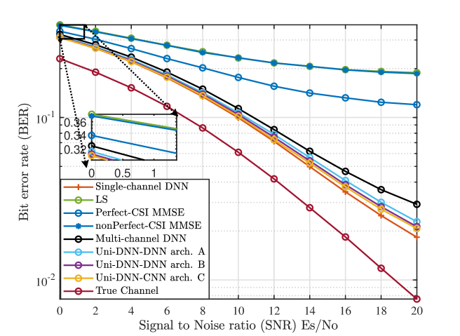
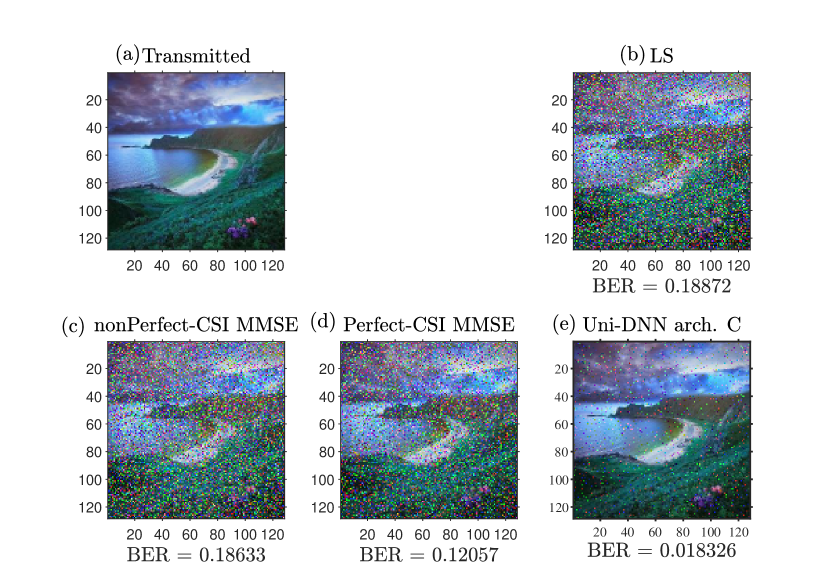
Fig. 2 shows that employing Uni-DNN architectures A, B and C outperforms both conventional and multi-channel DL model and closes the gap in BER performance to the single-channel trained DL model for 3GPP TDL-A channel at high SNR. For instance, Fig. 3 shows 3GPP TDL-A channel image detection example at 20dB SNR where Uni-DNN arch. C achieves a BER of while LS and perfect-CSI MMSE achieve and respectively. Also, we can see that feeding the classification as flattened 2D-grid input in arch. B and employing CNN in arch. C have further enhanced the BER performance compared to arch. A. This improvement can be linked to Uni-DNN arch. B and C’s per-channel weights assignment discussed earlier in section III-B. Although the channel classifier facilitated performance enhancement for all Uni-DNN architectures at high SNR in the case of 3GPP TDL-A channel, such enhancement is less apparent at low SNR due to misclassification of the channel as WINNER II since the two channels are correlated.
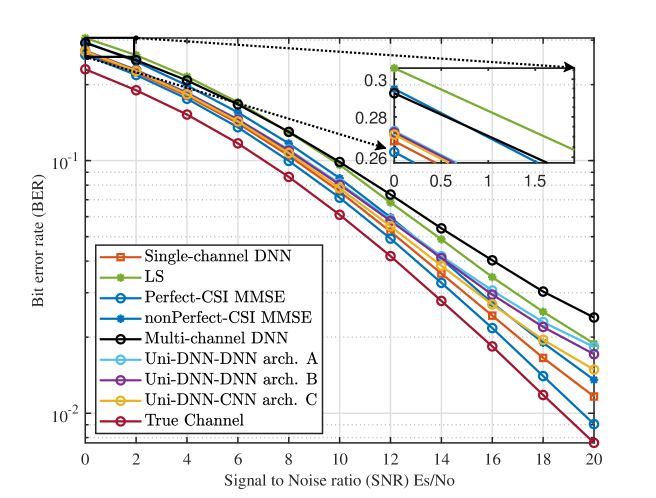
For the simulated Rician channel model, we can see from Fig. 5 and Fig. 6 that due to an insufficient number of pilots to estimate and interpolate a highly selective channel with 6 taps the performance of LS, perfect and non-perfect-CSI MMSE are poor and much inferior compared to DL models. Similar observations to the previous channel model can be seen but unlike the 3GPP TDL-A channel, the Rician channel has been correctly classified in high and low SNR which maintained the Uni-DNN architectures’ BER advantage across the whole SNR range. This accuracy can be attributed to the presence of a LOS component in the Rician channel, which exhibits a non-random pattern that is distinguishable compared to other channels. Overall, increasing the number of pilots reduces the performance gap between conventional methods and DL models, as well as closing the gap between all DL models and true channel BER performance curve as in Fig. 4 and Fig. 7.
IV-C Experimental Computational Complexity Comparison
In addition to the analytical computational complexity analysis discussed in subsection III-C, in this section, the inference time relative to the LS channel estimator for each method is shown in Table V. The experimental relative runtime results are obtained on hardware running Python on NVIDIA RTX-3060 GPU and generation i7 Intel CPU with 16GB of RAM. we can see that the experimental results are consistent with the analytical results in Table I.
| Model/Parameter | Inference Relative runtime |
| LS∗ | |
| MMSE | |
| Single-channel | |
| Multi-channel | |
| Uni-Arc-A∗∗ | |
| Uni-Arc-B∗∗ | |
| Uni-Arc-C∗∗ |
∗Excluding linear interpolation **Including channel classifier
V Conclusion
In this article, three universal cascaded DL-based models are proposed for joint channel estimation and signal detection. These models have shown better adaption to various channel models compared to DL models employing one DNN trained on multi-channels. Also, Uni-DNN architecture C has managed to minimize the gap in BER performance with single-channel trained DL models outperforming conventional estimation methods for various channel models without the requirement of re-training. Uni-DNN models have faster inference capability compared to MMSE estimators making it attractive for practical real-time applications as a universal basestation receiver. Simulating the proposed Uni-DNN on more complex scenarios such as pilotless or multiple-input-multiple-output OFDM or implementing it on hardware to verify the simulation results can be done as future work.
References
- [1] W. Y. Y. Yong Soo Cho, Jaekwon Kim, MIMO‐OFDM Wireless Communications with MATLAB®. John Wiley & Sons, Ltd, 2010.
- [2] M. K. Ozdemir and H. Arslan, “Channel estimation for wireless ofdm systems,” IEEE Communications Surveys & Tutorials, vol. 9, no. 2, pp. 18–48, Jul. 2007.
- [3] J.-J. van de Beek, O. Edfors, M. Sandell, S. Wilson, and P. Borjesson, “On channel estimation in ofdm systems,” in 1995 IEEE 45th Vehicular Technology Conference. Countdown to the Wireless Twenty-First Century, vol. 2, Jul. 1995, pp. 815–819 vol.2.
- [4] H. Ye, G. Y. Li, and B.-H. Juang, “Power of deep learning for channel estimation and signal detection in ofdm systems,” IEEE Wireless Communications Letters, vol. 7, no. 1, pp. 114–117, Sept. 2018.
- [5] Y. Yang, F. Gao, X. Ma, and S. Zhang, “Deep learning-based channel estimation for doubly selective fading channels,” IEEE Access, vol. 7, pp. 36 579–36 589, Mar. 2019.
- [6] X. Ma, H. Ye, and Y. Li, “Learning assisted estimation for time- varying channels,” in 2018 15th International Symposium on Wireless Communication Systems (ISWCS), 2018, pp. 1–5.
- [7] P. Chen and H. Kobayashi, “Maximum likelihood channel estimation and signal detection for ofdm systems,” in 2002 IEEE International Conference on Communications. Conference Proceedings. ICC 2002 (Cat. No.02CH37333), vol. 3, 2002, pp. 1640–1645 vol.3.
- [8] Z. Luo, Y. Zhan, and E. Jonckheere, “Analysis on functions and characteristics of the rician phase distribution,” in 2020 IEEE/CIC International Conference on Communications in China (ICCC), 2020, pp. 306–311.
- [9] Technical Specification Group Radio Access Network; Study on channel model for frequencies from 0.5 to 100 GHz (Release 14), 3rd Generation Partnership Project (3GPP), 12 2017, v14.3.0.
- [10] P. Kyösti, J. Meinilä, L. Hentila, X. Zhao, T. Jämsä, C. Schneider, M. Narandzi’c, M. Milojevi’c, A. Hong, J. Ylitalo, V.-M. Holappa, M. Alatossava, R. Bultitude, Y. Jong, and T. Rautiainen, “Ist-4-027756 winner ii d1.1.2 v1.2 winner ii channel models,” Journal of the Association for Information Science and Technology, vol. 11, 02 2008.