Ultralight scalar dark matter versus non-adiabatic perfect fluid dark matter in pulsar timing
Abstract
Recent evidence of direct detection of stochastic gravitational waves reported by pulsar timing array collaborations might open a new window for studying cosmology and astrophysical phenomena. In addition to signals from gravitational waves, there is motivation to explore residual signals from oscillating dark matter, which might partially comprise the galactic halo. We investigate fluctuations in pulsar timing originating from the coherent oscillation of scalar dark matter up to the subleading order of , as well as from acoustic oscillations of non-adiabatic perfect fluid dark matter. Both types of dark matter can generate oscillating Newtonian potential perturbations and curvature perturbations, thereby affecting pulsar timing. Our results show distinctive signatures in pulsar timing residuals and angular correlations for these dark matters. Specifically, pulsar timing residuals from non-adiabatic perfect fluid dark matter exhibit different directional dependence and are shown to be more sensitive to the distance to a pulsar. We also study the angular correlation patterns from these dark matters in the NANOGrav 15-year data set. The best fit might suggest that the composition of non-adiabatic perfect fluid dark matter in our galaxy is much greater than that of ultralight scalar dark matter.
I introduction
Recent evidence of direct detection of gravitational waves in nHz frequency bands might open a new window for studying cosmology in the early universe and astrophysical phenomena on sub-galactic scales, as reported by pulsar timing array (PTA) collaborations Xu et al. (2023); Zic et al. (2023); Smarra et al. (2023); Antoniadis et al. (2023a, b, c, d); Reardon et al. (2023); Agazie et al. (2023a, b); Afzal et al. (2023); Agazie et al. (2023c, d). A notable aspect of these experiments is that pulsar timing has the capacity to reflect metric perturbations via spatially correlated signals, such as the Hellings-Downs (HD) curve Hellings and Downs (1983). This capability enables the distinction of gravitational waves from other types of fluctuations Lee et al. (2008), including those originating from dark matter Khmelnitsky and Rubakov (2014); Antoniadis et al. (2023d); Afzal et al. (2023).
Dark matter plays a crucial role in modern cosmology and astrophysical physics. While the standard cosmological model, known as the Lambda cold dark matter (CDM) model, has been well-tested through observations such as the cosmic microwave background Aghanim et al. (2020) and large-scale structure Hinshaw et al. (2013), it appears to be inconsistent with observations on sub-galactic scales Weinberg et al. (2015). As an alternative candidate, ultralight scalar dark matter exhibits little difference from CDM on large scales but behaves as warm dark matter on small scales, potentially resolving discrepancies with small-scale observations Khmelnitsky and Rubakov (2014); Hlozek et al. (2015); Marsh (2016). A decade ago, it was found that pulsar timing could be influenced by the coherent oscillation of ultralight scalar field at a frequency proportional to its mass Khmelnitsky and Rubakov (2014). Consequently, it was expected that dark matter signals could be detected in PTA data sets Porayko and Postnov (2014); Porayko et al. (2018); Kato and Soda (2020); Kaplan et al. (2022). Recent studies have extended to ultralight vector dark matter Nomura et al. (2020); Xue et al. (2022); Wu et al. (2022); Sun et al. (2022); Unal et al. (2022) and ultralight tensor dark matter Armaleo et al. (2020); Sun et al. (2022); Unal et al. (2022); Wu et al. (2023). Although the detectability of ultralight dark matter has been elucidated in pioneer studies, there has been rare investigation into similar mechanisms for CDM (formulated by a perfect fluid with ). Hence, the primary motivation of this paper is to explore the potential oscillatory features of CDM that might have an effect on pulsar timing.
It is noteworthy that there are two competitive mechanisms regarding how ultralight dark matter affects pulsar timing: i) interaction between dark matter and normal matter Graham et al. (2016); Armaleo et al. (2020); Kaplan et al. (2022); Xue et al. (2022); Sun et al. (2022); Unal et al. (2022), and ii) self-interaction of gravity Khmelnitsky and Rubakov (2014); Aoki and Soda (2016); Porayko et al. (2018); Kato and Soda (2020); Nomura et al. (2020); Wu et al. (2022); Sun et al. (2022); Unal et al. (2022); Wu et al. (2023). In the latter, one should expand the Einstein field equation sourced by dark matter perturbatively to the second order. Therefore, it is a secondary and nonlinear effect. In the situation of , the pulsar timing residual from mechanism ii) reduces to the same form as that from mechanism i), but has different interpretations for the timing residual amplitudes and frequencies. Specifically, in mechanism i), the amplitude is proportional to the coupling constant, whereas in mechanism ii), it is proportional to the dark matter density. For ultralight dark matter with mass , the timing residual frequency in mechanism i) is , while it is in mechanism ii).
In this study, we investigate the pulsar timing residuals influenced by scalar dark matter and non-adiabatic perfect fluid dark matter within the framework of mechanism ii), employing a more rigorous formalism. For scalar dark matter, this formalism enables us to extensively calculate timing residuals to the subleading order of . It is found that the timing residual has directional dependence due to the subleading terms. For perfect fluid dark matter, we derive the equation of state parameter and set the effective sound speed , in order to let it serve as a type of CDM under non-adiabatic conditions Arena et al. (2006); Buldgen et al. (2015); Hu and Sijacki (2016). In this scenario, it is found that acoustic oscillations of perfect fluid dark matter should occur within our galaxy. Consequently, the oscillation can generate metric perturbations, influencing pulsar timing. Notably, the timing residual is found to be sensitive to the distance to a pulsar, distinguishable from the results obtained for scalar dark matter. In this sense, pulsar timing might offer a way to discern whether dark matter in our galaxy is adiabatic or not.
Due to the oscillations of dark matter throughout space, there could be a non-zero spatial correlation of timing residuals for a pulsar pair Armaleo et al. (2020). Specifically, by spatially averaging all pairs of pulsars at a given angular separation, one can derive the angular correlation Allen (2023). Recently, the angular correlations resulting from ultralight dark matters have also been referred to as deformed Hellings-Downs curves Omiya et al. (2023); Cai et al. (2024). Alternatively, one can employ the ensemble-average approach by considering the scalar field amplitude as a stochastic variable Luu et al. (2024); Kim and Mitridate (2024). These approaches yield consistent angular correlations theoretically. For example, the usages of both approaches for gravitational waves were comprehensively presented in Ref. Allen (2023). In this study, we adopt the ensemble-average approach and focus on the angular correlations originating from the coherent oscillation of scalar dark matter to the subleading order, as well as from the acoustic oscillation of non-adiabatic perfect fluid dark matter, separately. It shows that the angular correlations for these oscillating dark matters also have distinctive signatures.
The rest of the paper is organized as follows. In Sec. II, we compute the metric perturbations generated by scalar dark matter and perfect fluid dark matter, separately, based on the expansion of the Einstein field equation to the second order. In Sec. III, we obtain the response functions for the oscillating dark matters on pulsar timing by utilizing perturbed geodesic equations. In Sec. IV, we compute the timing residuals and angular correlations resulting from these oscillating dark matters, investigating their distinctive signatures. In Sec. V, we study the angular correlation patterns from these oscillating dark matters in the NANOGrav 15-year data set. Finally, in Sec. VI, conclusions and discussions are summarized.
II Metric perturbions generated by oscillating dark matters
In this section, we will derive and solve the equations of motion for the metric perturbations, which originate from the coherent oscillation of scalar dark matter and from the acoustic oscillation of perfect fluid dark matter, separately. For scalar dark matter, pioneering work derived results in the limit of Khmelnitsky and Rubakov (2014). Here, we will extend the calculation to the subleading order.
The perturbed Minkowski metric to the second order in the Newtonian gauge is given by
| (1) |
where is the second-order vector perturbation, is the second-order tensor perturbation, and and are the th-order Newtonian potential perturbation and curvature perturbation, respectively. Here, we set because the dark matter would not generate first-order vector or tensor perturbations. In the following, we will consider the metric perturbations sourced by two distinctive types of dark matter: scalar dark matter and perfect fluid dark matter.
II.1 Ultralight scalar dark matter
The energy-momentum tensor of the scalar field is given by where is the scalar field mass, and is the covariant derivative. The scalar field can be expanded in the form of . Here, we have due to the background being set to Minkowski spacetime. Expanding the energy-momentum tensor conservation to the second order, one can obtain the equation of motion for the scalar field, namely,
| (2) |
where denotes the Laplace operator, and ′ denotes the time derivative. The above equation of motion suggests that the scalar field oscillates in both space and time. By employing the expansion of , one can derive the first-order Einstein field equation, which yields a trivial solution . Subsequently, evaluating the second-order Einstein field equations in space-space components, we obtain
| (3a) | |||||
| (3b) | |||||
| (3c) | |||||
| (3d) | |||||
where we have employed the helicity decomposition, is the transverse-traceless operator, is the Einstein gravitational constant, and
| (4) |
It shows that Eqs. (3) do not involve the second-order scalar field . And the scalar, vector, and tensor metric perturbations are all generated by the scalar field .
Here, we consider the solution of Eq. (2) in the form of a plane wave expansion, namely
| (5) |
where . The Fourier mode of in Eq. (5) takes the form
| (6) |
Substituting Eq. (6) into Eqs. (3) and evaluating in Fourier space, we obtain the metric perturbations in the form of
| (7a) | |||||
| (7b) | |||||
| (7c) | |||||
where we have neglected the non-oscillatory parts. In the cases of , we can expand the above solutions as follows,
| (8a) | |||||
| (8b) | |||||
| (8c) | |||||
| (8d) | |||||
where
| (9a) | |||||
| (9b) | |||||
| (9c) | |||||
The Fourier modes , , and can all be derived from the scalar field, indicating that they are not independent of each other. Since the leading order of the -expansion was obtained in pioneer study Khmelnitsky and Rubakov (2014), we extend it to the subleading order. It seems that the vector perturbation is left to take the subleading-order effect.
II.2 Non-adiabatic perfect fluid dark matter
The energy-momentum tensor of the perfect fluid is given by , where the density , pressure , and velocity flow can be expanded in the form of
| (10) |
The is the equation of state parameter, and is the effective sound speed. Because the background is an exact Minkowski space-time in Eq. (1), it seems meaningless to define and .
Expanding the conservation of energy-momentum tensor to the first order, we obtain
| (11) |
Here, we adopt the scenario where and is stationary, which corresponds to the existence of dark matter density comprising the galactic halo. It is also consistent with the picture that perfect fluid dark matter can serve as a type of CDM within our galaxy. Expanding the conservation of the energy-momentum tensor in the second order, we obtain
| (12) |
Evaluating the above equation, we have
| (13) |
For non-adiabatic perfect fluid, , and is an independent quantity from the equation of state parameter . The wave equation in Eq. (13) suggests the presence of acoustic oscillations of the density perturbation within our galaxy.
Evaluating Einstein field equations to the second order, we obtain
| (14) |
and
| (15a) | |||||
| (15b) | |||||
| (15c) | |||||
| (15d) | |||||
where
| (16) |
Associating Eq. (11) and (14), we obtain a time-independent , consequently leading to in Eq. (16) being time-independent. Here, we focus on the oscillatory feature potentially reflected by pulsar timing. Thus, Eqs. (15) are evaluated by neglecting the non-oscillatory parts, namely,
| (17) |
It shows that only the Newtonian potential perturbation and the curvature perturbation can be generated by the oscillating perfect fluid dark matter. Based on Eq. (15), should satisfy the wave equation in the form of Eq. (13). Therefore, one can obtain the solution of and in Fourier modes, namely,
| (18) |
The above solutions also take the form of a plane wave expansion similar to Eq. (6). Because , if the non-adiabatic perfect fluid dark matter has an imprint on pulsar timing, the wavenumber in Eq. (18) should be much larger than the wavenumber for scalar dark matter in Eqs. (8).
The scalar dark matter density should be derived from the time average of due to . Consequently, the amplitude of the metric perturbations can be expressed in terms of the dark matter density Khmelnitsky and Rubakov (2014). However, no such relation exists for non-adiabatic perfect fluid dark matter. In this case, the amplitude in Eq. (18) and the corresponding density are independent quantities.
III reponse functions from gravitational fluctuations
The radio beam from PTAs propagates along geodesics in space. In the presence of space-time fluctuations between the pulsar and the earth, the fluctuations should leave an imprint on pulsar timing, which can be formulated as the perturbed geodesic equations, namely,
| (19) |
where and are the 4-velocity and perturbed 4-velocity of the radio beams. With the metric Eq. (1), one can obtain the solution of in Eq. (19) as follows,
| (20) | |||||
where we have introduced the direction vector , representing the location of a pulsar, and the second equality is obtained by making use of . Here, we denote the event of a radio beam emitted by a pulsar as , where represents the distance from earth to the pulsar, and the event of the observatory on earth receiving the radio signal as . Our result given in Eq. (20) is consistent with Eq. (20.58) of Ref. Maggiore (2018), while the Newtonian potential in Eq. (20) was neglected in Eq. (3.2) of Ref. Khmelnitsky and Rubakov (2014). Nevertheless, the neglect does not affect the conclusion of Ref. Khmelnitsky and Rubakov (2014).
In order to reflect the space-time fluctuations from the coherent oscillation of scalar dark matter, we compute the redshift between pulsar pulses by substituting Eqs. (6) and (7) into Eq. (20), namely,
| (21) | |||||
where the response functions are given by
| (22) |
and and have been defined in Eqs. (9a) and (9b). Here, we have expanded the results for a small and restrict our attention to the subleading order of . It is found that the vector perturbation does not affect the redshift, despite shown in Eq. (8c).
Similarly, we obtain the redshift originating from the acoustic oscillation of perfect fluid dark matter by making use of Eq. (18) and (20), namely
| (23) |
where the response function is given by
| (24) |
Differed from Eq. (21), the above result is exact. The response functions in Eq. (22) and Eq. (24) tend to be constant as or , indicating no directional dependence in these situations. In the next section, we will consider observables on PTAs by making use of the response functions.
IV Time residuals and angular correlations
IV.1 Time residuals
For the metric perturbations oscillating in a specific direction and at a specific frequency, one can consider with a characteristic wavenumber Maggiore (2007). In this case, the redshifts can be evaluated by making use of the real and positive frequency parts of Eqs. (21) and (23), namely,
| (25) | |||||
| (26) |
Following the approaches used in Ref. Khmelnitsky and Rubakov (2014), we further calculate the time residuals by integrating over time and neglecting the non-oscillatory part, namely,
| (27a) | |||||
| (27b) | |||||
where the amplitudes of the time residuals are
| (28a) | |||||
| (28b) | |||||
| (28c) | |||||
It is found that there are distinctive directional dependences in the amplitudes of these dark matters.
Figure 1 shows the directional dependence of in polar coordinates. The regime for the scalar dark matter implies . Hence, we consider to present its directional dependence. As shown in Figure 1, one might find that . As expected, the amplitude tends to be isotropic as . And the degree of directional dependence is determined by the value of .
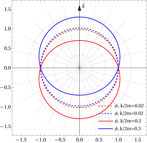
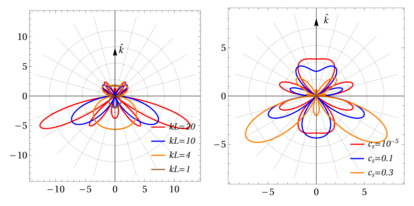
Figure 2 shows the directional dependence of . Similar to , the sound speed can determine the degree of directional dependence. Moreover, the amplitude also depends on . As increases, the amplitude enhances, and the number of the leaf in curves increases. By expanding the around with a finite , one can obtain
| (29) |
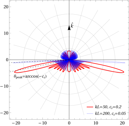
Since the amplitude at is enhanced with , we also show the amplitudes for a large in Figure 3. Theoretically, its directional dependence can be distinguished from that of the scalar dark matter.
IV.2 Angular correlations
In this part, we will compute angular correlations using the ensemble-average approach, considering metric perturbations as stochastic variables. In this sense, we can assume spectra of metric perturbations originating from the coherent oscillation of scalar dark matter in the form of
| (30a) | |||||
| (30b) | |||||
| (30c) | |||||
Non-vanishing cross-correlation exists between the metric perturbations and , since these perturbations are all generated from the scalar field , as shown in Eqs. (9a) and (9b). Further illustration on the power spectra is presented in Appendix B. Similarly, for the power spectrum originating from the acoustic oscillation of perfect fluid dark matter, we consider
| (31) |
Utilizing the correlations in Eqs. (30) and (31), we can derive the redshift correlation for pulsar pairs. For illustration, we formally express the redshift from pulsar as
| (32) |
where is response function, and the ensemble average of takes the form of . For the redshift correlation between a pulsar pair and , we evaluate it as
| (33) | |||||
where terms involving a multiplication of vanish due to the usage of time averaging Allen (2023). And the angular correlation for the output on the PTAs is given by
| (34) |
Herein, one can obtain the angular correlations from coherent ocillation of scalar dark matter, and from acoustic oscillation of perfect fluid dark matter by employing Eq. (34).
For the scalar dark matter with reshift given in Eq. (21), the angular correlations are
| (35a) | |||||
| (35b) | |||||
where
| (36) | |||||
For the non-adiabatic perfect fluid dark matter with reshift given in Eq. (23), the angular correlation is
| (37) |
where
| (38) | |||||
It shows that in Eqs. (36) and (38) exhibit distinct directional dependence. As and tend to zero, the oscillates with respect to , whereas tends to be independent of . For the latter case, we can compute the angular correlations by letting , namely,
| (39a) | |||||
| (39b) | |||||
It is found that the angular correlation is no longer uniform over angular separations due to the subleading order effect of .
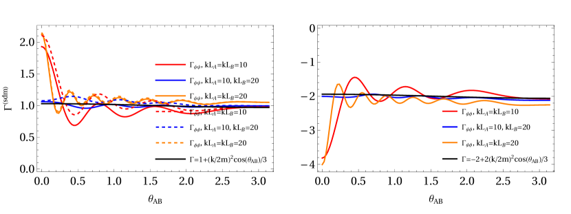
Figure 4 shows the angular correlation curves for scalar dark matter. These angular correlation curves in Eq. (36) oscillate around the black solid curves. This behavior resembles the angular correlations for gravitational wave backgrounds on PTAs Maggiore (2018), where the pulsar terms are not important. By comparing the solid and dashed curves on the left-hand side of Figure 4, it is also found that oscillatory feature of the curves can distinguish and .
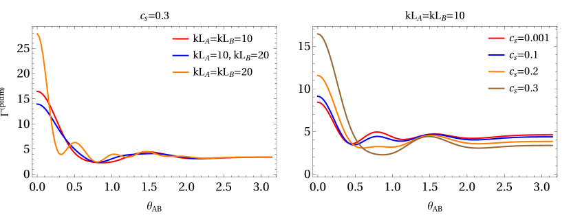
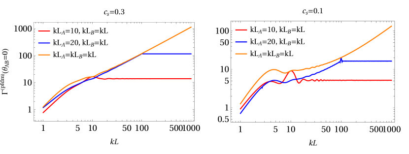
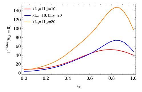
Figure 5 shows the angular correlations for given and . It is found that the value of at increases with . It might suggest that the enhancement could lead to an improvement in sensitivity for PTAs to the dark matter. We present as a function of and in Figure 6. In the case where , is shown to monotonically increase with . If either or is fixed, there exists an upper bound for . We also present as a function of in Figure 7. It shows that increases with small values of and decreases with larger values of . The turning points of the curves seem to be determined by .
V Potential Dark matter singlas in the angular correlation with NANOGrav 15-year data set
It is expected that the time residuals at the angular frequencies or in Eqs. (27) are within the PTA frequency bands. Hence, for a given distance to a pulsar , the for the scalar dark matter should be much smaller than 1, while the for the perfect fluid dark matter is much larger than 1. In these situations, the angular correlation for scalar dark matter tends to be constant, while the angular correlation for perfect fluid dark matter still has oscillatory behavior. Therefore, there should be distinctive signatures in angular correlations on PTAs.
Under the assumption that the output signals of PTAs originate from a combination of stochastic gravitational background, ultralight scalar dark matter, and non-adiabatic perfect fluid dark matter, the output per frequency bin can be formulated as
| (40) | |||||
We do not suspect that the stochastic gravitational waves should dominate the output signals on the PTAs. Instead, we explore the possibility of the existence of dark matter signals in angular correlations. Hence, we introduce the residual signals as follows,
| (41) |
where , , and we have used the conclusion that the angular correlations for the scalar dark matter tend to be constant shown in Eqs. (39). The is expected to be a positive number, which is shown in Appendix B.
The NANOGrav collaboration recently reported evidence of stochastic gravitational waves with their 15-year data set Agazie et al. (2023a), wherein alternative model-independent correlation patterns were also studied. Here, we consider the deformed angular correlations from the oscillating dark matter with the data set. Figure 8 shows the fit of the NANOGrav 15-year data set with the curves in Eq. (41). We have set . The best fit yields the following parameters: , , , and . The error variance is determined to be .
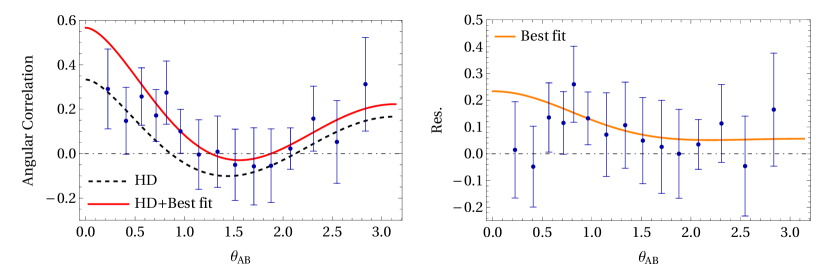
The and should be interpreted as the averaged distances of all pulsar pairs across the sky. The might imply that the composition of non-adiabatic perfect fluid dark matter is much greater than that of ultralight scalar dark matter. Nevertheless, we can not conclude the existence of acoustic oscillations of perfect fluid dark matter based on the data set due to parameter errors. It is expected that future data sets with higher precision will offer further insights into this study.
VI Conclusions and discussions
This study investigated the fluctuations in pulsar timing originating from the coherent oscillation of scalar dark matter up to the subleading order of , as well as from the acoustic oscillation of non-adiabatic perfect fluid dark matter based on the self-interaction of gravity. The distinctive signatures in pulsar timing residuals and angular correlations were presented for these two types of dark matter. Specifically, the pulsar timing residual from non-adiabatic perfect fluid dark matter was shown to be sensitive to the distance to a pulsar, while that for scalar dark matter is not. In PTA frequency bands, the angular correlation from the scalar dark matter tends to be constant, while the angular correlation from the perfect fluid dark matter still has oscillatory behavior with respect to or . We thus studied these angular correlation patterns in NANOGrav 15-year data set by subtracting the stochastic gravitational wave signals. The best fit might suggest that the composition of non-adiabatic perfect fluid dark matter in our galaxy is much greater than that of ultralight scalar dark matter, due to .
For scalar dark matter, due to the subleading terms of , timing residuals have directional dependence, and the angular correlations on PTAs are no longer uniform with respect to the angle separation. In the presence of non-adiabatic perfect fluid dark matter in our galaxy, we first found that the acoustic oscillations should occur. Consequently, these oscillations can generate metric perturbations, influencing pulsar timing. Theoretically, pulsar timing might also offer a way to discern whether dark matter in our galaxy is adiabatic or not.
Acknowledgments. The author thanks Prof. Qing-Guo Huang for useful discussions in the early stages of this work. This work is supported by the National Natural Science Foundation of China under grant No. 12305073.
Appendix A Comment on the usage of insteand of
The stochastic gravitational wave can be given by Romano and Cornish (2017); Maggiore (2018)
| (42) |
And it can be derived from the plane wave expansion of , namely,
| (43) |
by extending the range of wavenumber into the domain Maggiore (2007). However, this trick does not work in general. One can consider a plane expansion with dispersion relation , namely,
| (44) |
It can be evaluated to be
One might find that Eq. (LABEL:A4) can be further evaluated in the form of Eq. (42), only if . For the scalar dark matter, we have , thereby . Namely, the plane wave expansion describing the solution of scalar dark matter can not be evaluated in the form of Eq. (42). Hence, we utilize the momentum k instead of in this paper.
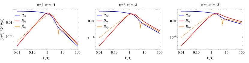
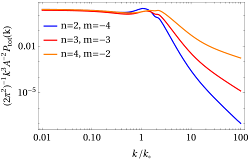
Appendix B Power spectrum of metric perturbations derived from the scalar dark matter
Based on Eqs. (9b) and (9a), the power spectra , and can all be derived with a given spectrum of the scalar field . Following the scenario of assuming a stochastic background for the scalar dark matter Luu et al. (2024); Kim and Mitridate (2024), one might have two-point function in the form of
| (46) |
By making use of the above two-point correlation, we obtain the power spectra for the metric perturbations and , namely,
| (47) | |||||
| (48) | |||||
| (49) |
Employing the in the form of
| (52) |
we compute the power spectrum , and numerically. Figure 9 shows these power spectra of the metric perturbations for selected indices and . As the scalar dark matter can contribute to the signal residuals in Eq. (41) with the , we also present the in Figure 10. It is found that is positive over the frequency.
References
- Xu et al. (2023) H. Xu et al., Res. Astron. Astrophys. 23, 075024 (2023), arXiv:2306.16216 [astro-ph.HE] .
- Zic et al. (2023) A. Zic et al., Publ. Astron. Soc. Austral. 40, e049 (2023), arXiv:2306.16230 [astro-ph.HE] .
- Smarra et al. (2023) C. Smarra et al. (European Pulsar Timing Array), Phys. Rev. Lett. 131, 171001 (2023), arXiv:2306.16228 [astro-ph.HE] .
- Antoniadis et al. (2023a) J. Antoniadis et al. (EPTA, InPTA), Astron. Astrophys. 678, A49 (2023a), arXiv:2306.16225 [astro-ph.HE] .
- Antoniadis et al. (2023b) J. Antoniadis et al. (EPTA, InPTA:), Astron. Astrophys. 678, A50 (2023b), arXiv:2306.16214 [astro-ph.HE] .
- Antoniadis et al. (2023c) J. Antoniadis et al. (EPTA), (2023c), arXiv:2306.16226 [astro-ph.HE] .
- Antoniadis et al. (2023d) J. Antoniadis et al. (EPTA), (2023d), arXiv:2306.16227 [astro-ph.CO] .
- Reardon et al. (2023) D. J. Reardon et al., Astrophys. J. Lett. 951, L6 (2023), arXiv:2306.16215 [astro-ph.HE] .
- Agazie et al. (2023a) G. Agazie et al. (NANOGrav), Astrophys. J. Lett. 951, L8 (2023a), arXiv:2306.16213 [astro-ph.HE] .
- Agazie et al. (2023b) G. Agazie et al. (NANOGrav), Astrophys. J. Lett. 952, L37 (2023b), arXiv:2306.16220 [astro-ph.HE] .
- Afzal et al. (2023) A. Afzal et al. (NANOGrav), Astrophys. J. Lett. 951, L11 (2023), arXiv:2306.16219 [astro-ph.HE] .
- Agazie et al. (2023c) G. Agazie et al. (NANOGrav), Astrophys. J. Lett. 956, L3 (2023c), arXiv:2306.16221 [astro-ph.HE] .
- Agazie et al. (2023d) G. Agazie et al. (NANOGrav), Astrophys. J. Lett. 951, L50 (2023d), arXiv:2306.16222 [astro-ph.HE] .
- Hellings and Downs (1983) R. w. Hellings and G. s. Downs, Astrophys. J. Lett. 265, L39 (1983).
- Lee et al. (2008) K. J. Lee, F. A. Jenet, and R. H. Price, Astrophys. J. 685, 1304 (2008).
- Khmelnitsky and Rubakov (2014) A. Khmelnitsky and V. Rubakov, JCAP 02, 019 (2014), arXiv:1309.5888 [astro-ph.CO] .
- Aghanim et al. (2020) N. Aghanim et al. (Planck), Astron. Astrophys. 641, A6 (2020), [Erratum: Astron.Astrophys. 652, C4 (2021)], arXiv:1807.06209 [astro-ph.CO] .
- Hinshaw et al. (2013) G. Hinshaw et al. (WMAP), Astrophys. J. Suppl. 208, 19 (2013), arXiv:1212.5226 [astro-ph.CO] .
- Weinberg et al. (2015) D. H. Weinberg, J. S. Bullock, F. Governato, R. Kuzio de Naray, and A. H. G. Peter, Proc. Nat. Acad. Sci. 112, 12249 (2015), arXiv:1306.0913 [astro-ph.CO] .
- Hlozek et al. (2015) R. Hlozek, D. Grin, D. J. E. Marsh, and P. G. Ferreira, Phys. Rev. D 91, 103512 (2015), arXiv:1410.2896 [astro-ph.CO] .
- Marsh (2016) D. J. E. Marsh, Phys. Rept. 643, 1 (2016), arXiv:1510.07633 [astro-ph.CO] .
- Porayko and Postnov (2014) N. K. Porayko and K. A. Postnov, Phys. Rev. D 90, 062008 (2014), arXiv:1408.4670 [astro-ph.CO] .
- Porayko et al. (2018) N. K. Porayko et al., Phys. Rev. D 98, 102002 (2018), arXiv:1810.03227 [astro-ph.CO] .
- Kato and Soda (2020) R. Kato and J. Soda, JCAP 09, 036 (2020), arXiv:1904.09143 [astro-ph.HE] .
- Kaplan et al. (2022) D. E. Kaplan, A. Mitridate, and T. Trickle, Phys. Rev. D 106, 035032 (2022), arXiv:2205.06817 [hep-ph] .
- Nomura et al. (2020) K. Nomura, A. Ito, and J. Soda, Eur. Phys. J. C 80, 419 (2020), arXiv:1912.10210 [gr-qc] .
- Xue et al. (2022) X. Xue et al. (PPTA), Phys. Rev. Res. 4, L012022 (2022), arXiv:2112.07687 [hep-ph] .
- Wu et al. (2022) Y.-M. Wu, Z.-C. Chen, Q.-G. Huang, X. Zhu, N. D. R. Bhat, Y. Feng, G. Hobbs, R. N. Manchester, C. J. Russell, and R. M. Shannon (PPTA), Phys. Rev. D 106, L081101 (2022), arXiv:2210.03880 [astro-ph.CO] .
- Sun et al. (2022) S. Sun, X.-Y. Yang, and Y.-L. Zhang, Phys. Rev. D 106, 066006 (2022), arXiv:2112.15593 [astro-ph.CO] .
- Unal et al. (2022) C. Unal, F. R. Urban, and E. D. Kovetz, (2022), arXiv:2209.02741 [astro-ph.CO] .
- Armaleo et al. (2020) J. M. Armaleo, D. López Nacir, and F. R. Urban, JCAP 09, 031 (2020), arXiv:2005.03731 [astro-ph.CO] .
- Wu et al. (2023) Y.-M. Wu, Z.-C. Chen, and Q.-G. Huang, JCAP 09, 021 (2023), arXiv:2305.08091 [hep-ph] .
- Graham et al. (2016) P. W. Graham, D. E. Kaplan, J. Mardon, S. Rajendran, and W. A. Terrano, Phys. Rev. D 93, 075029 (2016), arXiv:1512.06165 [hep-ph] .
- Aoki and Soda (2016) A. Aoki and J. Soda, Phys. Rev. D 93, 083503 (2016), arXiv:1601.03904 [hep-ph] .
- Arena et al. (2006) S. E. Arena, G. Bertin, T. Liseikina, and F. Pegoraro, Astron. Astrophys. 453, 9 (2006), arXiv:astro-ph/0603503 .
- Buldgen et al. (2015) G. Buldgen, D. R. Reese, M. A. Dupret, and R. Samadi, Astronomy & Astrophysics 574, A42 (2015).
- Hu and Sijacki (2016) S. Hu and D. Sijacki, Mon. Not. Roy. Astron. Soc. 461, 2789 (2016), arXiv:1507.01643 [astro-ph.GA] .
- Allen (2023) B. Allen, Phys. Rev. D 107, 043018 (2023), arXiv:2205.05637 [gr-qc] .
- Omiya et al. (2023) H. Omiya, K. Nomura, and J. Soda, Phys. Rev. D 108, 104006 (2023), arXiv:2307.12624 [astro-ph.CO] .
- Cai et al. (2024) R.-G. Cai, J.-R. Zhang, and Y.-L. Zhang, (2024), arXiv:2402.03984 [gr-qc] .
- Luu et al. (2024) H. N. Luu, T. Liu, J. Ren, T. Broadhurst, R. Yang, J.-S. Wang, and Z. Xie, Astrophys. J. Lett. 963, L46 (2024), arXiv:2304.04735 [astro-ph.HE] .
- Kim and Mitridate (2024) H. Kim and A. Mitridate, Phys. Rev. D 109, 055017 (2024), arXiv:2312.12225 [hep-ph] .
- Maggiore (2018) M. Maggiore, Gravitational Waves. Vol. 2: Astrophysics and Cosmology (Oxford University Press, 2018).
- Maggiore (2007) M. Maggiore, Gravitational Waves. Vol. 1: Theory and Experiments (Oxford University Press, 2007).
- Romano and Cornish (2017) J. D. Romano and N. J. Cornish, Living Rev. Rel. 20, 2 (2017), arXiv:1608.06889 [gr-qc] .