Estimation of the long-run variance of nonlinear time series with an application to change point analysis

Abstract

For a broad class of nonlinear time series known as Bernoulli shifts, we establish the asymptotic normality of the smoothed periodogram estimator of the long-run variance. This estimator uses only a narrow band of Fourier frequencies around the origin and so has been extensively used in local Whittle estimation. Existing asymptotic normality results apply only to linear time series, so our work substantially extends the scope of the applicability of the smoothed periodogram estimator. As an illustration, we apply it to a test of changes in mean against long-range dependence. A simulation study is also conducted to illustrate the performance of the test for nonlinear time series.

Keywords: Nonlinear time series, Long-run variance, Periodogram.

MSC 2020 subject classification:  62M10; 62M15.

1 Introduction

Over the past two decades, classical temporal dependence conditions based on cumulants or mixing coefficients have been complemented by conditions formulated in terms of nonlinear moving averages of the form

(1) $$X_{t}=g(\varepsilon_{t},\varepsilon_{t-1},\ldots),\ \ \ t\in\mathbb{Z},$$

where $g$ can be a fairly general function. Among them, the Physical or Functional Dependence and the Approximability have gained particular popularity and have been used in dozens of publications. Physical dependence was introduced by Wu [31] and studied or assumed in Wu and Mielniczuk [32], Liu et al. [22], Zhou [37], Zhang and Wu [35], Dette et al. [11] and van Delft [29], among many others. Approximability was also used in a large number of papers, for example, in Aue et al. [2], Hörmann and Kokoszka [15], Berkes et al. [8], Horváth et al. [16], Horváth et al. [17], Kokoszka et al. [19], Zhang [36], Bardsley et al. [5] and Horváth et al. [18].

Estimation of the spectral density function, which includes estimation of the long-run variance (LRV), is a key problem in time series analysis that has been studied for several decades. Specialized to the estimation of the LRV, the lag window estimator,

(2) $$\hat{f}(0)=\frac{1}{2\pi}\sum_{|r|\leq\ell_{n}}w\left(\frac{r}{\ell_{n}}\right)\hat{\gamma}_{r},$$

where the $\hat{\gamma}_{r}$ are the usual sample autocovariances, has been particularly extensively studied. Anderson [1] developed its theory for linear processes, while Rosenblatt [26] considered strong mixing processes satisfying cumulant summability conditions. These results were extended to nonlinear time series. Chanda [10] assumed a specific form of the general Bernoulli shifts (1), namely (for a fixed $w$), $X_{t}=\varepsilon_{t}+\sum_{r=1}^{\infty}g_{r}(\varepsilon_{t-1},\ldots,\varepsilon_{t-r-w}),$ with summability conditions on the fourth moments of the $g_{r}(\varepsilon_{t-1},\ldots,\varepsilon_{t-r-w})$. The above representation is motivated by a truncated Volterra expansion. Results of Shao and Wu [27], Wu and Shao [33], and Liu and Wu [21], which assume only the general representation (1), can be specialized to yield asymptotic normality of the estimator (2) under various conditions related to the physical dependence of Wu [31].

In this paper, we consider the smoothed periodogram estimator

(3) $$Q_{n}=\frac{1}{m}\sum_{j=1}^{m}I_{n}(\omega_{j}),$$

where $I_{n}(\omega_{j})$ is the periodogram at the Fourier frequency $\omega_{j}$ and $m$ is the count of frequencies used in the estimation ($m/n\to 0$). While the lag window estimator (2) can be expressed as a weighted sum of the periodogram over all Fourier frequencies, estimator (3) uses only a narrow band of local Fourier frequencies. For this reason, it is particularly relevant in local Whittle estimation, see e.g. Robinson [24], Velasco [30], Phillips and Shimotsu [23], Robinson [25], Baek and Pipiras [3], Li et al. [20] and Baek et al. [4]. The asymptotic distribution of the estimator (3) is only available under the assumption of linearity, see Giraitis et al. [13] for the most up to date comprehensive account. In this paper, we establish its asymptotic normality for general nonlinear moving averages and present an application to change point analysis. We note that Brillinger [9] considers an estimator similar to (3) (see his equation (6.6)), but for a fixed $m$, and (3) is not even consistent then.

The paper is organized as follows. In Section 2, we introduce the objects we study. Section 3 contains the main theorems, while Section 4 presents an application to change point analysis. All proofs are collected in Section 5. Graphs and Tables of a small simulation study validating our asymptotic theory in finite samples are presented in online Supporting Information.

2 Preliminaries

2.1 The spectral density and the periodogram

We assume in the following that $\{X_{t}\}_{t\in\mathbb{Z}}$ is a strictly stationary sequence of real random variables satisfying

$$\operatorname{E}X_{1}=0\quad\text{and}\quad\operatorname{E}X_{1}^{2}<\infty.$$

Let $\{\gamma(h)\}_{h\in\mathbb{Z}}$ be the sequence of autocovariances of $\{X_{t}\}_{t\in\mathbb{Z}}$, where $\gamma(h)=\operatorname{Cov}(X_{h},X_{0})$ for $h\in\mathbb{Z}$. The spectral density function of the series $\{X_{t}\}_{t\in\mathbb{Z}}$ is defined by

(4) $$f(\omega)=\frac{1}{2\pi}\sum_{h=-\infty}^{\infty}\gamma(h)e^{-ih\omega},\ \ \ \omega\in[-\pi,\pi].$$

The discrete Fourier transform (DFT) of $X_{1},\ldots,X_{n}$ and the periodogram are defined by

(5) $$\mathcal{X}_{n}(\omega_{j})=\frac{1}{\sqrt{2\pi n}}\sum_{t=1}^{n}X_{t}e^{-it\omega_{j}}\ \ \ \text{and}\ \ \ I_{n}(\omega_{j})=|\mathcal{X}_{n}(\omega_{j})|^{2}$$

with the Fourier frequencies $\omega_{j}=2\pi j/n$, where $j\in\{-\lfloor(n-1)/2\rfloor,\ldots,\lfloor n/2\rfloor\}$ and $\lfloor\cdot\rfloor$ is the floor function.

2.2 Weak dependence

Let $\{X_{t}\}_{t\in\mathbb{Z}}$ be a sequence of real random variables of the form (1), where $\{\varepsilon_{t}\}_{t\in\mathbb{Z}}$ is a sequence of independent and identically distributed (iid) random elements in a measurable space $S$ and $g:S^{\infty}\to\mathbb{R}$ is a measurable function. Series of the form (1) are often called Bernoulli shifts and are automatically strictly stationary.

Suppose that $\{\varepsilon_{t}^{\prime}\}_{t\in\mathbb{Z}}$ is an independent copy of $\{\varepsilon_{t}\}_{t\in\mathbb{Z}}$. Define $X_{t,\{0\}}$ by replacing $\varepsilon_{0}$ in (1) by $\varepsilon_{0}^{\prime}$, i.e.,

(6) $$X_{t,\{0\}}=g(\varepsilon_{t},\ldots,\varepsilon_{1},\varepsilon_{0}^{\prime},\varepsilon_{-1},\ldots),\ \ \ t\in\mathbb{Z}.$$

We write $X\in\mathcal{L}^{p}$ with $p>0$ if $\|X\|_{p}=(\operatorname{E}|X|^{p})^{1/p}<\infty$. The physical dependence measure is defined by

(7) $$\delta_{t,p}=\|X_{t}-X_{t,\{0\}}\|_{p},\ \ \ t\in\mathbb{Z}.$$

Observe that $\delta_{t,p}=0$ if $t<0$. Even though $\delta_{t,p}$ can be considered for any positive value of $p$, typically $p\geq 1$ is assumed since otherwise $\|\cdot\|_{p}$ is no longer a norm (we will work with $p=4$). According to Definition 3 of Wu [31], $\{X_{t}\}_{t\in\mathbb{Z}}$ is called $p$-strong stable if

(8) $$\Theta_{p}=\sum_{t=0}^{\infty}\delta_{t,p}<\infty,\ \ \ p\geq 1.$$

Wu [31] also considers the case when instead of replacing $\varepsilon_{0}$ with its independent copy, $\varepsilon_{t}$’s in (1) with indices in some index set $I\subset\mathbb{Z}$ are replaced with their independent copies. If all but the first $m$ $\varepsilon_{t}$’s in (1) are replaced with their independent copies, we obtain the concept of $L^{p}$-$m$-approximability studied by Hörmann and Kokoszka [14] in the setting of functional time series. More precisely, let

(9) $$X_{t}^{(m)}=g(\varepsilon_{t},\ldots,\varepsilon_{t-m+1},\varepsilon_{t-m}^{\prime},\varepsilon_{t-m-1}^{\prime},\ldots).$$

We say that $\{X_{t}\}_{t\in\mathbb{Z}}$ is $L^{p}$-$m$-approximable if

(10) $$\sum_{t=1}^{\infty}\|X_{t}-X_{t}^{(t)}\|_{p}<\infty,\ \ \ p\geq 1,$$

see Definition 2.1 of Hörmann and Kokoszka [14]. Observe that $\|X_{t}-X_{t}^{(t)}\|_{p}=\|X_{s}-X_{s}^{(t)}\|_{p}$ for $s,t\in\mathbb{Z}$ so that the right-hand side of (10) can be formulated solely in terms of $X_{1}$ and the approximations $X_{1}^{(t)}$ with $t\geq 1$.

The following lemma establishes that $L^{p}$-$m$-approximability implies $p$-strong stability.

Lemma 1.

The inequality

(11) $$\delta_{t,p}=\|X_{t}-X_{t,\{0\}}\|_{p}\leq 2\|X_{t}-X_{t}^{(t)}\|_{p}$$

holds for $t\geq 1$ and $p\geq 1$ with $X_{t}$, $X_{t,\{0\}}$, and $X_{t}^{(t)}$ given by (1), (6), and (9), respectively.

Proof of Lemma 1.

The proof essentially follows from the proof of Lemma 3.0^⋆ of van Delft [28] (see page 5 therein), but we give it here for the sake of convenience (the published version, van Delft [29], does not contain this lemma).

Denote the $\sigma$-algebras generated by the random elements $\varepsilon_{t},\varepsilon_{t-1},\ldots$ with $t\in\mathbb{Z}$ and $\varepsilon_{t},\ldots,\varepsilon_{s}$ with $t\geq s$ by $\mathcal{F}_{t}=\sigma(\varepsilon_{t},\varepsilon_{t-1},\ldots)$ and $\mathcal{F}_{t,s}=\sigma(\varepsilon_{t},\ldots,\varepsilon_{s})$, respectively. We have that

$$\|X_{t}-X_{t,\{0\}}\|_{p}\leq\|X_{t}-\operatorname{E}[X_{t}\mid\mathcal{F}_{t,1}]\|_{p}+\|\operatorname{E}[X_{t}\mid\mathcal{F}_{t,1}]-X_{t,\{0\}}\|_{p}.$$

Since $\{\varepsilon_{t}^{\prime}:t\in\mathbb{Z}\}$ is an independent copy of $\{\varepsilon_{t}:t\in\mathbb{Z}\}$,

$$\operatorname{E}[X_{t}\mid\mathcal{F}_{t,1}]=\operatorname{E}[X_{t}^{(t)}\mid\mathcal{F}_{t,1}]=\operatorname{E}[X_{t}^{(t)}\mid\mathcal{F}_{t}]$$

almost surely and hence

(12) $$\|X_{t}-\operatorname{E}[X_{t}\mid\mathcal{F}_{t,1}]\|_{p}=\|\operatorname{E}[X_{t}\mid\mathcal{F}_{t}]-\operatorname{E}[X_{t}^{(t)}\mid\mathcal{F}_{t}]\|_{p}\leq\|X_{t}-X_{t}^{(t)}\|_{p}$$

using Jensen’s inequality for conditional expectations with $p\geq 1$. We conclude the proof by noticing that $\operatorname{E}[X_{t}\mid\mathcal{F}_{t,1}]$ does not depend on $\varepsilon_{0}$ and hence

$$\|\operatorname{E}[X_{t}\mid\mathcal{F}_{t,1}]-X_{t,\{0\}}\|_{p}=\|\operatorname{E}[X_{t}\mid\mathcal{F}_{t,1}]-X_{t}\|_{p},$$

which is bounded in the same way as in (12). The proof is complete. ∎

Remark 1.

The $L^{p}$-$m$-approximability is in fact strictly stronger than $p$-strong stability. Consider, for example, a linear process $\{X_{t}\}_{t\in\mathbb{Z}}$, where $X_{t}=\sum_{j=0}^{\infty}\psi_{j}\varepsilon_{t-j}$ for $t\in\mathbb{Z}$, $\{\varepsilon_{t}\}_{t\in\mathbb{Z}}$ is a sequence of iid random variables such that $\operatorname{E}\varepsilon_{0}=0$ and $\operatorname{E}\varepsilon_{0}^{2}<\infty$, while $\{\psi_{j}\}_{j\geq 0}$ is a sequence such that $\sum_{j=0}^{\infty}\psi_{j}^{2}<\infty$. Observe that

$$\sum_{t=0}^{\infty}\|X_{t}-X_{t,\{0\}}\|_{2}=2^{1/2}\|\varepsilon_{0}\|_{2}\sum_{t=0}^{\infty}|\psi_{t}|\quad\text{and}\quad\sum_{t=1}^{\infty}\|X_{t}-X_{t}^{(t)}\|_{2}=2^{1/2}\|\varepsilon_{0}\|_{2}\sum_{t=1}^{\infty}\Bigl{(}\sum_{j=t}^{\infty}\psi_{j}^{2}\Bigr{)}^{1/2}.$$

Suppose that $\psi_{j}=(j+1)^{-d}$ for $j\geq 0$ with some $d>1$. Then

$$\Bigl{(}\sum_{j=t}^{\infty}\psi_{j}^{2}\Bigr{)}^{1/2}\sim\frac{t^{1/2-d}}{(2d-1)^{1/2}}\quad\text{as}\quad t\to\infty.$$

So $\{X_{t}\}_{t\in\mathbb{Z}}$ is $2$-strong stable for any value of $d>1$ but $\{X_{t}\}_{t\in\mathbb{Z}}$ is $L^{2}$-$m$-approximable only if $d>3/2$.

3 Estimation of the long-run variance

Consider the time series $\{X_{t}\}_{t\in\mathbb{Z}}$ and its spectral density $f$, both defined in Section 2.1. The long-run variance of $\{X_{t}\}_{t\in\mathbb{Z}}$ is defined as

$$\tau_{X}:=\sum_{k=-\infty}^{\infty}\gamma(h)=2\pi f(0).$$

The estimation of $\tau_{X}$ can thus be reduced to the estimation of $f(0)$, and this approach is commonly used. A natural estimator of $f(0)$, known as the smoothed periodogram or the nonparametric spectral estimator given by (3). The chief contribution of this paper is showing that the estimator $Q_{n}$ is asymptotically normal, with the rate $m^{-1/2}$, for a broad class of nonlinear moving averages of the form (1). We work under the following general assumption.

Assumption 1.

The series $\{X_{t}\}_{t\in\mathbb{Z}}$ admits representation (1) and for some $\kappa>3$,

(13) $$\|X_{t}-X_{t}^{(m)}\|_{4}=O(m^{-\kappa}),\ \ \ {\rm as}\ m\to\infty.$$

Assumption 1 implies the that

(14) $$\sum_{h=1}^{\infty}h^{r}|\gamma(h)|<\infty,\ \ \ 0\leq r<\kappa-1,$$

because, as in the proof of Lemma 4.1 of Hörmann and Kokoszka [14],

$$\sum_{h=1}^{\infty}|h|^{r}|\gamma(h)| =\sum_{h=1}^{\infty}|h|^{r}|\operatorname{Cov}(X_{0},X_{h}-X_{h}^{(h)})+\operatorname{Cov}(X_{0},X_{h}^{(h)})|$$

$$\leq\|X_{0}\|_{2}\sum_{h=1}^{\infty}|h|^{r}\|X_{h}-X_{h}^{(h)}\|_{2}$$

$$\leq\|X_{0}\|_{2}\sum_{h=1}^{\infty}|h|^{r}\|X_{h}-X_{h}^{(h)}\|_{4}.$$

Since Assumption 1 implies (14), which in turn implies the absolute summability of the autocovariances, $f(0)$ is well-defined under Assumption 1.

Theorem 1.

Assume that $\operatorname{E}X_{0}=0$, $\operatorname{E}|X_{0}|^{4}<\infty$, Assumption 1 holds and $m=m_{n}\to\infty$, but $m=o(n^{4/5})$, as $n\to\infty$. Then

(15) $$\frac{\sqrt{m}}{f(0)}[Q_{n}-f(0)]=\frac{1}{\sqrt{m}}\sum_{j=1}^{m}\biggl{(}\frac{I_{n}(\omega_{j})}{f(0)}-1\biggr{)}\xrightarrow{d}\mathcal{N}(0,1),\ \ \ {\rm as}\ n\to\infty,$$

where $Q_{n}$ is defined in (3) and $f(0)$ in (4).

Theorem 1 follows from Theorems 2 and 3 formulated below. We decompose the sequence in (15) into two terms

(16) $$\frac{\sqrt{m}}{f(0)}[Q_{n}-f(0)]=\frac{\sqrt{m}}{f(0)}(Q_{n}-\operatorname{E}Q_{n})+\frac{\sqrt{m}}{f(0)}(\operatorname{E}Q_{n}-f(0)).$$

Theorem 2, which implies that the first term on the right-hand side of (16) converges to $\mathcal{N}(0,1)$ in distribution, is established under much weaker assumptions than Theorem 1. In particular, the $L^{p}$-$m$-approximability of Assumption 1 is replaced by the weaker $p$-strong stability (by Lemma 1, Assumption 1 implies that $\Theta_{4}<\infty$). Furthermore, only the weakest possible assumption on the rate of $m$ is imposed in Theorem 2 (Assumption 2 below). We need to impose a stronger assumption on the growth rate of $m$ in Theorem 1 than in Theorem 2 to ensure that the second term on the right-hand side of (16) is asymptotically negligible. Assumption 1 implies that $\sum_{h=1}^{\infty}h^{2}\gamma(h)<\infty$ and hence, according to Theorem 3, $\operatorname{E}Q_{n}-f(0)=O(\max\{n^{-1},(m/n)^{2}\})$, as $n\to\infty$. The assumption in Theorem 1 that $m=o(n^{4/5})$ as $n\to\infty$ then implies that $\sqrt{m}(m/n)^{2}=(m/n^{4/5})^{5/4}=o(1)$, as $n\to\infty$.

Observe that (15) implies that

(17) $$\frac{1}{m}\sum_{j=1}^{m}\biggl{(}\frac{I_{n}(\omega_{j})}{f(0)}-1\biggr{)}=O_{p}(m^{-1/2}),\ \ \ {\rm as}\ n\to\infty.$$

Both (15) and (17) are used in theoretical work related to the estimation of the long-run variance. We give an application in Section 4.

For ease of reference, we formulate the standard assumption on the growth rate of $m$.

Assumption 2.

As $n\to\infty$, $m\to\infty$, but $m=o(n)$.

Theorem 2.

Assume that $\operatorname{E}X_{0}=0$, $\operatorname{E}|X_{0}|^{4}<\infty$, $\Theta_{4}<\infty$ with $\Theta_{4}$ defined by (8), and Assumption 2 holds. Then

(18) $$\frac{\sqrt{m}}{f(0)}(Q_{n}-\operatorname{E}Q_{n})\xrightarrow{d}\mathcal{N}(0,1),\ \ \ {\rm as}\ n\to\infty,$$

where $Q_{n}$ is defined in (3) and $f(0)$ in (4).

The proof of Theorem 2 is given in Section 5. It relies on a general central limit theorem for quadratic forms established by Liu and Wu [21] (see Theorem 6 therein). The next theorem establishes that the rate at which the bias of the estimator $Q_{n}$ vanishes depends on the rate at which $\gamma(h)\to 0$, as $n\to\infty$.

Theorem 3.

Suppose that $\operatorname{E}X_{0}=0$, $\operatorname{E}X_{0}^{2}<\infty$, $\sum_{h=1}^{\infty}h^{r}|\gamma(h)|<\infty$ with some $r\geq 0$ and Assumption 2 holds. Then

$$\operatorname{E}Q_{n}-f(0)=\begin{cases}o(1)&\text{if}\ r=0,\\ O((m/n)^{r})&\text{if}\ 0<r\leq 1,\\ O(\max\{n^{-1},(m/n)^{\min\{2,r\}}\})&\text{if}\ r>1,\end{cases}$$

where $Q_{n}$ is defined in (3) and $f(0)$ in (4).

The proof of Theorem 3 is given in Section 5.

4 Application to change point analysis

A problem that has attracted some attention over the past twenty years is distinguishing between long memory, or long-range dependence (LRD), and changes in mean. Stationary time series used to model LRD exhibit spurious changes in mean that Benoit Mandelbrot called the Joseph effect, referring to periods of famine and plenty. This is a fundamental characteristic of all stationary long memory models, see e.g. Beran et al. [6]. Berkes et al. [7] proposed a significance test of the null hypothesis of changes in mean against a long memory alternative. They review earlier exploratory research on this problem. Under the null hypothesis, the observations $X_{t}$ satisfy

(19) $$X_{t}=\begin{cases}\mu+r_{t},&1\leq t\leq n^{\star},\\ \mu+\Delta+r_{t},&n^{\star}+1\leq t\leq N,\end{cases}$$

where $\mu$ is the base mean level, $\Delta$ the magnitude of change at an unknown change point $n^{\star}$ and $\{r_{t}\}_{t\in\mathbb{Z}}$ is a stationary, weakly dependent series. Berkes et al. [7] characterized the weak dependence of the $r_{t}$ by the convergence of their partial sums to the Wiener process and summability conditions on the autocovariances and fourth order cumulants. Their test is based on the maximum of two CUSUM statistics. Baek and Pipiras [3] pointed out that this test can have low power and proposed a more powerful test of (19) based on the local Whittle estimator (LWE) of the Hurst parameter, $H$. However, they could justify their procedure only for linear processes $\{r_{t}\}_{t\in\mathbb{Z}}$. They relied on results of Robinson [24] valid only for linear time series. We show in this section that the approach of Baek and Pipiras [3] is applicable also to nonlinear processes satisfying the assumptions of Theorem 1. All results of this Section are proven in Section 5.3.

We begin with the definition of the LWE of $H$.

Definition 1.

The LWE of the self-similarity (Hurst) parameter $H$ of the process $\{X_{t}\}$ is defined as

(20) $$\widehat{H}=\operatorname*{arg\,min}_{H\in\Theta}L(H),$$

where $\Theta=[\Delta_{1},\Delta_{2}]$ with $0<\Delta_{1}<\Delta_{2}<1$ and

(21) $$L(H)=\log\left(\frac{1}{m}\sum_{l=1}^{m}\omega_{l}^{2H-1}I_{n}(\omega_{l})\right)-(2H-1)\frac{1}{m}\sum_{l=1}^{m}\log\omega_{l}.$$

The following theorem is needed to establish the asymptotic distribution of $\widehat{H}$ under weak dependence ($H=1/2$).

Theorem 4.

Suppose $\operatorname{E}X_{0}=0$, $\operatorname{E}|X_{0}|^{4}<\infty$ and Assumption 1 holds. If

(22) $$\frac{1}{m}+\frac{m^{5}(\log m)^{2}}{n^{4}}\to 0,\quad{\rm as}\ n\to\infty,$$

then

$$\widetilde{Q}_{n}=\frac{1}{\sqrt{m}}\sum_{l=1}^{m}\nu_{l,m}\left(\frac{I_{n}(\omega_{l})}{f(0)}-1\right)\stackrel{{\scriptstyle\mbox{$\scriptstyle d$}}}{{\rightarrow}}{\cal N}(0,1),\quad{\rm as}\ n\to\infty,$$

where

$$\nu_{l,m}=\log l-\frac{1}{m}\sum_{j=1}^{m}\log j.$$

The next theorem plays a key role in justifying the test of Baek and Pipiras [3].

Theorem 5.

Under the assumptions of Theorem 4,

$$2\sqrt{m}\left(\widehat{H}-\frac{1}{2}\right)\stackrel{{\scriptstyle\mbox{$\scriptstyle d$}}}{{\rightarrow}}{\cal N}(0,1),\quad{\rm as}\ n\to\infty.$$

To construct the test statistic of Baek and Pipiras [3], the first step is to eliminate the effect of a potential change point that can severely bias the LWE. Consider the residuals

$$R_{t}=\begin{cases}X_{t}-\frac{1}{\hat{n}}\sum_{i=1}^{\hat{n}}X_{i},&1\leq t\leq\hat{n},\\ X_{t}-\frac{1}{N-\hat{n}}\sum_{i=\hat{n}+1}^{N}X_{i},&\hat{n}+1\leq t\leq N,\end{cases}$$

where $\hat{n}$ is a change point estimator. We use the standard CUSUM estimator

$$\hat{n}=\min\left\{k:\left|\sum_{j=1}^{k}X_{j}-\frac{k}{N}\sum_{j=1}^{N}X_{j}\right|=\max_{1\leq s\leq N}\left|\sum_{j=1}^{s}X_{j}-\frac{s}{N}\sum_{j=1}^{N}X_{j}\right|\right\}.$$

Motivated by Theorem 5, the test statistic is

(23) $$T^{(R)}=2\sqrt{m}\left(\widehat{H}^{(R)}-\frac{1}{2}\right),$$

where $\widehat{H}^{(R)}$ is the LWE based on the residual process $\{R_{t}\}$. The null hypothesis is rejected if $T^{(R)}>q_{1-\alpha}$, where $q_{1-\alpha}$ is the $(1-\alpha)$th quantile of the standard normal distribution. Theorem 6 justifies this rejection rule.

Theorem 6.

Suppose model (19) with the $r_{t}$ satisfying $\operatorname{E}r_{0}=0$, $\operatorname{E}|r_{0}|^{4}<\infty$ and Assumption 1. In addition, assume that
(i) $n^{\star}=\lfloor N\theta\rfloor$ for some $\theta\in(0,1)$;
(ii) the change in mean level $\Delta=\Delta(N)$ and the change point estimator $\hat{n}$ satisfy

$$N\Delta^{2}\to\infty,\quad\Delta^{2}\left|\hat{n}-n^{\star}\right|=O_{P}(1),\quad{\rm as}\ N\to\infty.$$

If

$$\frac{1}{m}+\frac{m^{5}(\log m)^{2}}{N^{4}}+\frac{m(\log m)^{2}}{N\Delta^{2}}\to 0,\quad{\rm as}\ N\to\infty,$$

then $T^{(R)}\stackrel{{\scriptstyle\mbox{$\scriptstyle d$}}}{{\rightarrow}}{\cal N}(0,1)$.

We conclude this section by reporting the results of a small simulation study that examines the finite sample behavior of the test statistic $T^{(R)}$ and the test based on it. We consider two non-linear processes used in modeling returns on financial assets. These models are not considered by Baek and Pipiras [3] and are not covered by their theory.

Definition 2.

The series $\{r_{t}\}$ is said to be a GARCH$(1,1)$ process if it satisfies the equations

(24) $$r_{t}=\sigma_{t}\epsilon_{t},\ \ \ \sigma_{t}^{2}=\alpha_{0}+\alpha_{1}r_{t-1}^{2}+\beta_{1}\sigma_{t-1}^{2},$$

where $\alpha_{0}>0$, $\alpha_{1},\beta_{1}\geq 0$, $\alpha_{1}+\beta_{1}<1$ and the $\epsilon_{t}$ are iid random variables with mean zero, unit variance and finite fourth moment.

The condition $\alpha_{1}+\beta_{1}<1$ implies that the GARCH$(1,1)$ process has a second-order stationary solution (which is also strictly stationary) with a representation of form (1). A necessary and sufficient condition for the existence of the fourth moments of the GARCH$(1,1)$ process is given by

(25) $$\operatorname{E}|\beta_{1}+\alpha_{1}\epsilon_{0}^{2}|^{2}<1$$

(we refer to Francq and Zakoian [12] for an extensive review of GARCH processes). Wu and Min [34] established (see Proposition 3 therein) that condition (25) also implies that the GARCH$(1,1)$ process satisfies the geometric-moment contraction (GMC) condition, i.e., $\operatorname{E}|r_{n}-r_{n}^{(n)}|^{4}\leq C\rho^{n}$, for some $C<\infty$ and $\rho\in(0,1)$, where $r_{n}^{(n)}$ is defined by (9) for $n\geq 1$. Hence, Assumption 1 is satisfied provided that condition (25) holds.

As the next example, we consider the simplest stochastic volatility model.

Definition 3.

The stochastic volatility (SV) model is given by

(26) $$r_{t}=\exp(x_{t}/2)\epsilon_{t},\ \ \ x_{t}=\alpha+\phi x_{t-1}+w_{t},$$

where $\alpha\in\mathbb{R}$, $|\phi|<1$, $w_{t}\stackrel{{\scriptstyle iid}}{{\sim}}\mathcal{N}(0,\sigma_{w}^{2})$, $\epsilon_{t}\stackrel{{\scriptstyle iid}}{{\sim}}\mathcal{N}(0,1)$ and $\{w_{t}\}$ and $\{\epsilon_{t}\}$ are mutually independent.

Proposition 1.

The $r_{t}$ specified in Definition 3 satisfy Assumption 1.

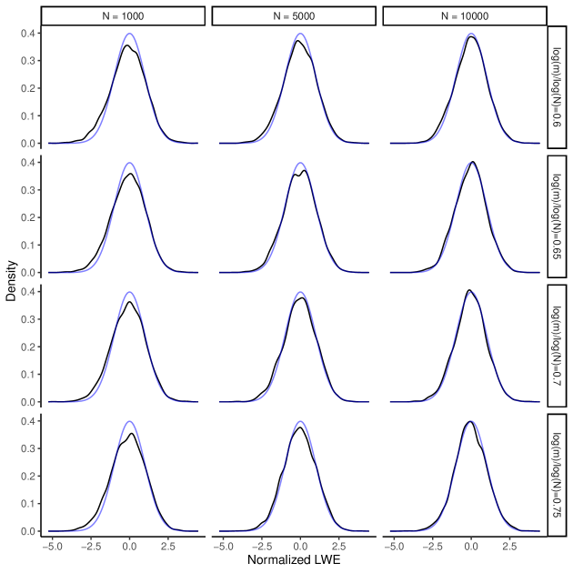
Figure 2: The same as Figure 1, but the $r_{t}$ follow SV model with $\alpha=0$, $\phi=0.5$ and $\sigma_{w}^{2}=1$.

We computed the empirical density functions of the normalized LWE based on $\{r_{t}\}$ for both models, which are displayed in Figures 1 and 2 presented in the Supporting Information. These figures show that the asymptotic normality established in Theorem 5 holds well in finite samples. We also evaluated the empirical size of the test based on Theorem 6. The results reported in Tables 1 and 2 in the Supporting Information show that these sizes are comparable with those obtained for linear processes.

5 Proofs of the results of Sections 3 and 4

We begin with a few auxiliary lemmas that isolate technical arguments from our main proofs.

5.1 Auxiliary lemmas

Lemma 2.

For $x,y\in\mathbb{R}$, $k,r\in\mathbb{Z}$, and $n\geq 1$,

$$\sum_{t=1}^{n}\cos((t-x)\omega_{k})\cos((t-y)\omega_{r})\\ =\begin{cases}\frac{n}{2}[\cos(x\omega_{k}-y\omega_{r})+\cos(x\omega_{k}+y\omega_{r})]&\text{if}\ k+r\in n\mathbb{Z}\ \text{and}\ k-r\in n\mathbb{Z};\\ \frac{n}{2}\cos(x\omega_{k}-y\omega_{r})&\text{if}\ k+r\in\mathbb{Z}\setminus n\mathbb{Z}\ \text{and}\ k-r\in n\mathbb{Z};\\ \frac{n}{2}\cos(x\omega_{k}+y\omega_{r})&\text{if}\ k+r\in n\mathbb{Z}\ \text{and}\ k-r\in\mathbb{Z}\setminus n\mathbb{Z};\\ 0&\text{if}\ k+r\in\mathbb{Z}\setminus n\mathbb{Z}\ \text{and}\ k-r\in\mathbb{Z}\setminus n\mathbb{Z}.\end{cases}$$

Proof.

Using the fact that $\cos x=(e^{ix}+e^{-ix})/2$ for $x\in\mathbb{R}$,

$$4\sum_{t=1}^{n}\cos((t-x)\omega_{k})\cos((t-y)\omega_{r})$$

$$=\sum_{t=1}^{n}(e^{i(t-x)\omega_{k}}+e^{-i(t-x)\omega_{k}})(e^{i(t-y)\omega_{r}}+e^{-i(t-y)\omega_{r}})$$

$$=e^{-i(x\omega_{k}+y\omega_{r})}\sum_{t=1}^{n}(e^{2\pi i/n})^{(k+r)t}+e^{-i(x\omega_{k}-y\omega_{r})}\sum_{t=1}^{n}(e^{2\pi i/n})^{(k-r)t}$$

$$\ \ \ +e^{i(x\omega_{k}-y\omega_{r})}\sum_{t=1}^{n}(e^{2\pi i/n})^{-(k-r)t}+e^{i(x\omega_{k}+y\omega_{r})}\sum_{t=1}^{n}(e^{2\pi i/n})^{-(k+r)t}.$$

We have that

$$e^{-i(x\omega_{k}+y\omega_{r})}\sum_{t=1}^{n}(e^{2\pi i/n})^{(k+r)t}+e^{i(x\omega_{k}+y\omega_{r})}\sum_{t=1}^{n}(e^{2\pi i/n})^{-(k+r)t}\\ =\begin{cases}2n\cos(x\omega_{k}+y\omega_{r})&\text{if}\ k+r\in n\mathbb{Z};\\ 0&\text{if}\ k+r\notin n\mathbb{Z}.\end{cases}$$

Similarly,

$$e^{-i(x\omega_{k}-y\omega_{r})}\sum_{t=1}^{n}(e^{2\pi i/n})^{(k-r)t}+e^{i(x\omega_{k}-y\omega_{r})}\sum_{t=1}^{n}(e^{2\pi i/n})^{-(k-r)t}\\ =\begin{cases}2n\cos(x\omega_{k}-y\omega_{r})&\text{if}\ k-r\in n\mathbb{Z};\\ 0&\text{if}\ k-r\notin n\mathbb{Z}.\end{cases}$$

The proof is complete. ∎

Lemma 3.

For $x,y\in\mathbb{R}$, $k,r\in\mathbb{Z}$, and $n\geq 1$,

$$\sum_{t=1}^{n}\sin((t-x)\omega_{k})\sin((t-y)\omega_{r})\\ =\begin{cases}\frac{n}{2}[\cos(x\omega_{k}-y\omega_{r})-\cos(x\omega_{k}+y\omega_{r})]&\text{if}\ k+r\in n\mathbb{Z}\ \text{and}\ k-r\in n\mathbb{Z};\\ \frac{n}{2}\cos(x\omega_{k}-y\omega_{r})&\text{if}\ k+r\in\mathbb{Z}\setminus n\mathbb{Z}\ \text{and}\ k-r\in n\mathbb{Z};\\ -\frac{n}{2}\cos(x\omega_{k}+y\omega_{r})&\text{if}\ k+r\in n\mathbb{Z}\ \text{and}\ k-r\in\mathbb{Z}\setminus n\mathbb{Z};\\ 0&\text{if}\ k+r\in\mathbb{Z}\setminus n\mathbb{Z}\ \text{and}\ k-r\in\mathbb{Z}\setminus n\mathbb{Z}.\end{cases}$$

The proof of Lemma 3 is analogous to the proof of Lemma 2 and thus is omitted.

Lemma 4.

Suppose that Assumption 2 holds. Then, for $j,l\in\mathbb{Z}$,

$$\sum_{t=1}^{n}a_{n,t-j}a_{n,t-l}=\frac{n}{2m}a_{n,j-l}$$

provided that $n$ is sufficiently large, where $a_{n,t}$ is given by (30) for $n\geq 1$ and $t\in\mathbb{Z}$.

Proof.

We have that

$$\sum_{t=1}^{n}a_{n,t-j}a_{n,t-l} =\frac{1}{m^{2}}\sum_{k=1}^{m}\sum_{r=1}^{m}\Bigl{\{}\sum_{t=1}^{n}\cos((t-j)\omega_{k})\cos((t-l)\omega_{r})\Bigr{\}}$$

$$=\frac{1}{m^{2}}\Bigl{[}\sum_{k=1}^{m}\Bigl{\{}\sum_{t=1}^{n}\cos((t-j)\omega_{k})\cos((t-l)\omega_{k})\Bigr{\}}+$$

$$\quad+\sum_{\begin{subarray}{c}k,r=1\\ k\neq r\end{subarray}}^{m}\Bigl{\{}\sum_{t=1}^{n}\cos((t-j)\omega_{k})\cos((t-l)\omega_{r})\Bigr{\}}\Bigr{]}$$

$$=\frac{1}{m^{2}}\sum_{k=1}^{m}\frac{n}{2}\cos((j-l)\omega_{k})$$

$$=\frac{n}{2m}a_{n,j-l}$$

using Lemma 2 since we have that (a) $2k\in\mathbb{Z}\setminus n\mathbb{Z}$for $k=1,\ldots,m$ provided that $n$ is sufficiently large due to Assumption 2; (b) $k-r\in\mathbb{Z}\setminus n\mathbb{Z}$and $k+r\in\mathbb{Z}\setminus n\mathbb{Z}$ when $k,r=1,\ldots,m$ and $k\neq r$ provided that $n$ is sufficiently large due to Assumption 2. The proof is complete. ∎

Lemma 5.

Let $\nu_{l,m}=\log l-\frac{1}{m}\sum_{j=1}^{m}\log j$. Then,

(27) $$\lim_{m\to\infty}\frac{1}{m}\sum_{k=1}^{m}\nu_{k,m}^{2}=1,$$

(28) $$\max_{1\leq k\leq m}|\nu_{k,m}|=O(\log m).$$

Proof.

Note that

$$\frac{1}{m}\sum_{k=1}^{m}\nu_{k,m}^{2}\sim\frac{1}{m}\sum_{k=1}^{m}\left(\log\left(\frac{k}{m}\right)+1\right)^{2}\to\int_{0}^{1}(\log x+1)^{2}dx=1.$$

Moreover, (28) follows directly from Lemma 2 in Robinson [24]. The proof is complete. ∎

5.2 Proofs of the theorems of Section 3

Proof of Theorem 2:.

Convergence in (18) follows from Theorem 6 of Liu and Wu [21] for $\lambda=0$. Since

$$I_{n}(\omega_{j})=\frac{1}{2\pi n}\sum_{s,t=1}^{n}X_{s}X_{t}\cos((s-t)\omega_{j})$$

for $n\geq 1$ and $j\in\{-\lfloor(n-1)/2\rfloor,\ldots,\lfloor n/2\rfloor\}$, $Q_{n}$ is thus a quadratic form

(29) $$Q_{n}=\frac{1}{2\pi n}\sum_{s,t=1}^{n}a_{n,s-t}X_{s}X_{t},$$

where $n\geq 1$,

(30) $$a_{n,t}=\frac{1}{m}\sum_{j=1}^{m}\cos(t\omega_{j})$$

and $t\in\mathbb{Z}$. Notice that $a_{n,t}=a_{n,-t}$ for $n\geq 1$ and $t\in\mathbb{Z}$, $a_{n,0}=1$ for $n\geq 1$ and $a_{n,t}\to 1$ as $n\to\infty$ for each $t\in\mathbb{Z}$ provided that Assumption 2 holds.

We establish that $\sqrt{m}(Q_{n}-\operatorname{E}Q_{n})\xrightarrow{d}\mathcal{N}(0,f^{2}(0))$ by showing that conditions (5.2) – (5.5) of Theorem 6 of Liu and Wu [21] hold. Using Lemma 4,

$$\sigma_{n}^{2}=2\cdot\frac{m}{4\pi^{2}n^{2}}\sum_{s=1}^{n}\sum_{t=1}^{n}a_{n,s-t}^{2}=2\cdot\frac{m}{4\pi^{2}n^{2}}\sum_{s=1}^{n}\frac{n}{2m}=\frac{1}{4\pi^{2}}$$

and

$$\varsigma_{n}^{2}=\frac{m}{4\pi^{2}n^{2}}\sum_{t=1}^{n}a_{n,t}^{2}=\frac{1}{8\pi^{2}n}.$$

for sufficiently large values of $n$.

We have that

$$\frac{m}{4\pi^{2}n^{2}}\max_{0\leq t\leq n}a_{n,t}^{2}\cdot\frac{1}{\varsigma_{n}^{2}}=\frac{m}{4\pi^{2}n^{2}}\max_{0\leq t\leq n}\Bigl{|}\frac{1}{m}\sum_{j=1}^{m}\cos(t\omega_{j})\Bigr{|}^{2}\cdot 8\pi^{2}n\leq\frac{2m}{n}\to 0$$

as $n\to\infty$ due to Assumption 2. Hence, condition (5.2) of Theorem 6 of Liu and Wu [21] holds. Also, $n\varsigma_{n}^{2}=(8\pi^{2})^{-1}$ for sufficiently large values of $n$ and thus $n\varsigma_{n}^{2}=O(\sigma_{n}^{2})$ as $n\to\infty$ which establishes condition (5.3) of Theorem 6 of Liu and Wu [21]. Using Lemma 4,

$$\sum_{k=1}^{n}\sum_{t=1}^{k-1}\Bigl{|}\sum_{j=1+k}^{n}\frac{\sqrt{m}a_{n,k-j}}{2\pi n}\frac{\sqrt{m}a_{n,t-j}}{2\pi n}\Bigr{|}^{2}$$

$$=\frac{m^{2}}{16\pi^{4}n^{4}}\sum_{k=1}^{n}\sum_{t=1}^{k-1}\Bigl{|}\sum_{j=1+k}^{n}a_{n,k-j}a_{n,t-j}\Bigr{|}^{2}$$

$$\leq\frac{m^{2}}{16\pi^{4}n^{4}}\sum_{k=1}^{n}\sum_{t=1}^{n}\Bigl{[}\sum_{j=1}^{n}a_{n,k-j}^{2}a_{n,t-j}^{2}+2\sum_{j=1+k}^{n-1}\sum_{l=j+1}^{n}a_{n,k-j}a_{n,t-j}a_{n,k-l}a_{n,t-l}\Bigr{]}$$

$$=\frac{m^{2}}{16\pi^{4}n^{4}}\Bigl{[}\sum_{j=1}^{n}\sum_{k=1}^{n}a_{n,k-j}^{2}\sum_{t=1}^{n}a_{n,t-j}^{2}+2\sum_{k=1}^{n}\sum_{j=1+k}^{n-1}\sum_{l=j+1}^{n}a_{n,k-j}a_{n,k-l}\Bigl{(}\sum_{t=1}^{n}a_{n,t-j}a_{n,t-l}\Bigr{)}\Bigr{]}$$

$$=\frac{m^{2}}{16\pi^{4}n^{4}}\Bigl{[}n\cdot\frac{n}{2m}\cdot\frac{n}{2m}+\frac{n}{m}\sum_{k=1}^{n}\sum_{j=1+k}^{n-1}a_{n,k-j}\Bigl{(}\sum_{l=j+1}^{n}a_{n,k-l}a_{n,j-l}\Bigr{)}\Bigr{]}$$

for sufficiently large values of $n$. We have that

$$\Bigl{|}\frac{n}{m}\sum_{k=1}^{n}\sum_{j=1+k}^{n-1}a_{n,k-j}\Bigl{(}\sum_{l=j+1}^{n}a_{n,k-l}a_{n,j-l}\Bigr{)}\Bigr{|}\leq\frac{n}{m}\sum_{k=1}^{n}\Bigl{|}\sum_{j=1+k}^{n-1}a_{n,k-j}\Bigl{(}\sum_{l=j+1}^{n}a_{n,k-l}a_{n,j-l}\Bigr{)}\Bigr{|}.$$

By the Cauchy-Schwarz inequality and Lemma 4,

$$\Bigl{|}\sum_{j=1+k}^{n-1}a_{n,k-j}\Bigl{(}\sum_{l=j+1}^{n}a_{n,k-l}a_{n,j-l}\Bigr{)}\Bigr{|} \leq\Bigl{(}\sum_{j=1+k}^{n-1}a_{n,k-j}^{2}\Bigr{)}^{1/2}\Bigl{(}\sum_{j=1+k}^{n-1}\Bigl{|}\sum_{l=j+1}^{n}a_{n,k-l}a_{n,j-l}\Bigr{|}^{2}\Bigr{)}^{1/2}$$

$$\leq\Bigl{(}\sum_{j=1}^{n}a_{n,k-j}^{2}\Bigr{)}^{1/2}\Bigl{(}\sum_{j=1}^{n}\Bigl{|}\sum_{l=j+1}^{n}a_{n,k-l}a_{n,j-l}\Bigr{|}^{2}\Bigr{)}^{1/2}$$

$$\leq\Bigl{(}\frac{n}{2m}\Bigr{)}^{1/2}\Bigl{(}\sum_{j=1}^{n}\sum_{l=j+1}^{n}a_{n,k-l}^{2}\sum_{l=j+1}^{n}a_{n,j-l}^{2}\Bigr{)}^{1/2}$$

$$\leq\Bigl{(}\frac{n}{2m}\Bigr{)}^{1/2}\Bigl{(}\sum_{j=1}^{n}\frac{n^{2}}{4m^{2}}\Bigr{)}^{1/2}$$

$$=\Bigl{(}\frac{n^{4}}{8m^{3}}\Bigr{)}^{1/2}$$

$$=\frac{n^{2}}{2\sqrt{2}m^{3/2}}.$$

Hence,

$$\Bigl{|}\frac{n}{m}\sum_{k=1}^{n}\sum_{j=1+k}^{n-1}a_{n,k-j}\Bigl{(}\sum_{l=j+1}^{n}a_{n,k-l}a_{n,j-l}\Bigr{)}\Bigr{|}\leq\frac{n}{m}\cdot n\cdot\frac{n^{2}}{2\sqrt{2}m^{3/2}}=\frac{n^{4}}{2\sqrt{2}m^{5/2}}$$

and condition (5.4) of Theorem 6 of Liu and Wu [21] holds. Finally, we show that condition (5.5) of Theorem 6 of Liu and Wu [21] holds. Using the identity

$$\cos\theta-\cos\varphi=-2\sin\Bigl{(}\frac{\theta+\varphi}{2}\Bigr{)}\sin\Bigl{(}\frac{\theta-\varphi}{2}\Bigr{)}$$

for $\theta,\varphi\in\mathbb{R}$ and Lemma 3,

$$\sum_{k=1}^{n}\Bigl{|}\frac{\sqrt{m}}{2\pi n}a_{n,k}-\frac{\sqrt{m}}{2\pi n}a_{n,k-1}\Bigr{|}^{2}$$

$$=\frac{1}{4\pi^{2}n^{2}m}\sum_{k=1}^{n}\Bigl{|}\sum_{j=1}^{m}\{\cos(k\omega_{j})-\cos((k-1)\omega_{j})\}\Bigr{|}^{2}$$

$$=\frac{1}{\pi^{2}n^{2}m}\sum_{k=1}^{n}\Bigl{|}\sum_{j=1}^{m}\sin\Bigl{(}\frac{(2k-1)\omega_{j}}{2}\Bigr{)}\sin\Bigl{(}\frac{\omega_{j}}{2}\Bigr{)}\Bigr{|}^{2}$$

$$=\frac{1}{\pi^{2}n^{2}m}\Bigl{\{}\sum_{j=1}^{m}\Bigl{[}\sum_{k=1}^{n}\sin^{2}((k-1/2)\omega_{j})\Bigr{]}\sin^{2}\Bigl{(}\frac{\omega_{j}}{2}\Bigr{)}$$

$$\quad+2\sum_{j=1}^{m-1}\sum_{l=j+1}^{m}\Bigl{[}\sum_{k=1}^{n}\sin((k-1/2)\omega_{j})\sin((k-1/2)\omega_{l})\Bigr{]}\sin\Bigl{(}\frac{\omega_{j}}{2}\Bigr{)}\sin\Bigl{(}\frac{\omega_{l}}{2}\Bigr{)}\Bigr{\}}$$

$$=\frac{1}{\pi^{2}n^{2}m}\Bigl{\{}\frac{n}{2}\sum_{j=1}^{m}\sin^{2}\Bigl{(}\frac{\omega_{j}}{2}\Bigr{)}\Bigr{\}}$$

$$=\frac{1}{2\pi^{2}nm}\sum_{j=1}^{m}\sin^{2}\Bigl{(}\frac{\omega_{j}}{2}\Bigr{)}$$

for sufficiently large values of $n$. Using the identities $\sin^{2}(\theta)=(1-\cos(2\theta))/2$ for $\theta\in\mathbb{R}$ and

$$\sum_{k=1}^{m}\cos(xk)=\frac{\sin(xm/2)\cos(x(m+1)/2)}{\sin(x/2)}$$

for $x\notin 2\pi\mathbb{Z}$ and $m\geq 1$,

$$\sum_{j=1}^{m}\sin^{2}\Bigl{(}\frac{\omega_{j}}{2}\Bigr{)} =\sum_{j=1}^{m}\frac{1-\cos(\omega_{j})}{2}$$

$$=\frac{1}{2}\Bigl{[}m-\sum_{j=1}^{m}\cos\Bigl{(}\frac{2\pi}{n}\cdot j\Bigr{)}\Bigr{]}$$

$$=\frac{1}{2}\Bigl{[}m-\frac{\sin(\pi m/n)\cos(\pi(m+1)/n)}{\sin(\pi/n)}\Bigr{]}$$

$$=\frac{m}{2}\Bigl{[}1-\frac{\sin(\pi m/n)/(\pi m/n)\cos(\pi(m+1)/n)}{\sin(\pi/n)/(\pi/n)}\Bigr{]}$$

$$=o(m)$$

as $n\to\infty$. Hence,

$$\frac{1}{\varsigma_{n}^{2}}\sum_{k=1}^{n}\Bigl{|}\frac{\sqrt{m}}{2\pi n}a_{n,k}-\frac{\sqrt{m}}{2\pi n}a_{n,k-1}\Bigr{|}^{2}=o(1)$$

as $n\to\infty$ as required. Theorem 6 of Liu and Wu [21] then implies that

$$\sigma_{n}^{-1}[\sqrt{m}(Q_{n}-\operatorname{E}Q_{n})]\xrightarrow{d}\mathcal{N}(0,4\pi^{2}f^{2}(0))$$

as $n\to\infty$ which in turn implies (18). The proof is complete. ∎

Proof of Theorem 3.

Observe that $Q_{n}$ can be expressed in the following way

(31) $$Q_{n}=\frac{1}{2\pi}\sum_{h=-(n-1)}^{n-1}a_{n,h}\hat{\gamma}(h)$$

for $n\geq 1$, where $a_{n,h}$ is defined by (30) for $n\geq 1$ and $h\in\mathbb{Z}$ while $\hat{\gamma}(h)$ are sample autocovariances given by

$$\hat{\gamma}(h)=\frac{1}{n}\sum_{j=1}^{n-h}X_{j+h}X_{j}$$

for $0\leq h<n$ and $\hat{\gamma}(h)=\hat{\gamma}(-h)$ for $-n<h\leq 0$. Hence, we have that

$$\operatorname{E}\biggl{[}\frac{1}{m}\sum_{j=1}^{m}I_{n}(\omega_{j})\biggr{]}-f(0)$$

$$=\frac{1}{2\pi}\sum_{h=-(n-1)}^{n-1}\Bigl{(}1-\frac{|h|}{n}\Bigr{)}\gamma(h)\biggl{[}\frac{1}{m}\sum_{j=1}^{m}\cos(h\omega_{j})\biggr{]}-\frac{1}{2\pi}\sum_{h=-\infty}^{\infty}\gamma(h)$$

$$=\frac{1}{2\pi}\biggl{[}\,\sum_{h=-(n-1)}^{n-1}\biggl{\{}\Bigl{(}1-\frac{|h|}{n}\Bigr{)}\biggl{[}\frac{1}{m}\sum_{j=1}^{m}\cos(h\omega_{j})\biggr{]}-1\biggr{\}}\gamma(h)-\sum_{|h|\geq n}\gamma(h)\biggr{]}$$

$$=\frac{1}{\pi}\biggl{[}\,\sum_{h=1}^{n-1}\biggl{\{}\biggl{[}\frac{1}{m}\sum_{j=1}^{m}\cos(h\omega_{j})\biggr{]}-\frac{h}{n}\biggl{[}\frac{1}{m}\sum_{j=1}^{m}\cos(h\omega_{j})\biggr{]}-1\biggr{\}}\gamma(h)-\sum_{h=n}^{\infty}\gamma(h)\biggr{]}$$

$$=\frac{1}{\pi}\biggl{[}\,\sum_{h=1}^{n-1}\biggl{\{}\biggl{[}\frac{1}{m}\sum_{j=1}^{m}\cos(h\omega_{j})\biggr{]}-1-\frac{h}{n}\biggl{[}\frac{1}{m}\sum_{j=1}^{m}\cos(h\omega_{j})\biggr{]}\biggr{\}}\gamma(h)-\sum_{h=n}^{\infty}\gamma(h)\biggr{]}.$$

Split the sum into two parts

(32) $$\sum_{h=1}^{n-1}\biggl{|}\frac{1}{m}\sum_{j=1}^{m}\cos(h\omega_{j})-1\biggr{|}|\gamma(h)|\\ =\sum_{h=1}^{\tau_{n,m}-1}\biggl{|}\frac{1}{m}\sum_{j=1}^{m}\cos(h\omega_{j})-1\biggr{|}|\gamma(h)|+\sum_{h=\tau_{n,m}}^{n-1}\biggl{|}\frac{1}{m}\sum_{j=1}^{m}\cos(h\omega_{j})-1\biggr{|}|\gamma(h)|,$$

where

$$\tau_{n,m}=\biggl{\lfloor}\frac{\sqrt{3}n}{\pi\sqrt{(m+1)(2m+1)}}\biggr{\rfloor}.$$

Using the mean value theorem and the fact that $|\sin x|\leq|x|$ for $x\in\mathbb{R}$,

$$\Bigl{|}\cos\Bigl{(}h\cdot\frac{2\pi j}{n}\Bigr{)}-\cos(0)\Bigr{|}=|\sin c|\Bigl{|}\frac{2\pi hj}{n}\Bigr{|}\leq\Bigl{|}\frac{2\pi hj}{n}\Bigr{|}^{2}$$

with some $c\in(0,2\pi hj/n)$. Hence,

$$\sum_{h=1}^{\tau_{n,m}-1}\biggl{|}\frac{1}{m}\sum_{j=1}^{m}\cos(h\omega_{j})-1\biggr{|}|\gamma(h)| \leq\sum_{h=1}^{\tau_{n,m}-1}\frac{2}{3}\Bigl{|}\frac{\pi h}{n}\Bigr{|}^{2}(m+1)(2m+1)|\gamma(h)|$$

(33) $$=\frac{2}{3}\Bigl{|}\frac{\pi}{n}\Bigr{|}^{2}(m+1)(2m+1)\sum_{h=1}^{\tau_{n,m}-1}h^{2}|\gamma(h)|.$$

If $0\leq r<2$,

$$\sum_{h=1}^{\tau_{n,m}-1}h^{2}|\gamma(h)|=\sum_{h=1}^{\tau_{n,m}-1}h^{2-r}h^{r}|\gamma(h)|\leq(\tau_{n,m}-1)^{2-r}\sum_{h=1}^{\tau_{n,m}-1}h^{r}|\gamma(h)|$$

and (33) is $O((m/n)^{r})$ as $n\to\infty$. If $r\geq 2$, (33) is $O((m/n)^{2})$ as $n\to\infty$. We bound the second term of (32) in the following way

$$\sum_{h=\tau_{n,m}}^{n-1}\biggl{|}\frac{1}{m}\sum_{j=1}^{m}\cos(h\omega_{j})-1\biggr{|}|\gamma(h)| \leq 2\sum_{h=\tau_{n,m}}^{n-1}|\gamma(h)|$$

$$=2\sum_{h=\tau_{n,m}}^{n-1}h^{-r}h^{r}|\gamma(h)|$$

$$\leq 2\tau_{n,m}^{-r}\sum_{h=\tau_{n,m}}^{n-1}h^{r}|\gamma(h)|$$

$$=o((m/n)^{r})$$

as $n\to\infty$. We have that

$$\sum_{h=1}^{n-1}\frac{h}{n}\biggl{|}\frac{1}{m}\sum_{j=1}^{m}\cos(h\omega_{j})\biggr{|}|\gamma(h)|\leq\frac{1}{n}\sum_{h=1}^{n-1}h|\gamma(h)|.$$

If $0<r<1$, then

$$\frac{1}{n}\sum_{h=1}^{n-1}h|\gamma(h)|=\frac{1}{n}\sum_{h=1}^{n-1}h^{1-r}h^{r}|\gamma(h)|\leq\frac{(n-1)^{1-r}}{n}\sum_{h=1}^{n-1}h^{r}|\gamma(h)|=O(n^{-r})$$

as $n\to\infty$. If $r\geq 1$, then

$$\frac{1}{n}\sum_{h=1}^{n-1}h|\gamma(h)|=O(n^{-1})$$

as $n\to\infty$. Finally,

$$\sum_{h=n}^{\infty}|\gamma(h)|=\sum_{h=n}^{\infty}h^{r}h^{-r}|\gamma(h)|\leq n^{-r}\sum_{h=n}^{\infty}h^{r}|\gamma(h)|=o(n^{-r})$$

as $n\to\infty$. The proof is complete. ∎

5.3 Proofs of the results of Section 4

Analogous to Theorem 2, the proof of Theorem 4 heavily relies on Theorem 6 of Liu and Wu [21]. So, we formulate a proposition which verifies that conditions (5.2)–(5.4) in Liu and Wu [21] are satisfied.

Proposition 2.

Define

$$\tilde{a}_{n,t}=\frac{1}{2\pi n\sqrt{m}}\sum_{l=1}^{m}\nu_{l,m}\cos(t\omega_{l}),$$

$$\widetilde{\sigma}_{n}^{2}=2\sum_{k=1}^{n}\sum_{t=1}^{n}\tilde{a}^{2}_{n,t-k},$$

and

$$\widetilde{\varsigma}^{2}_{n}=\sum_{t=1}^{n}\tilde{a}^{2}_{n,t}.$$

If

(34) $$\frac{m\log m}{n}\to 0,\quad\text{as }n\to\infty,$$

then, the following is true:
(i)

$$\max_{0\leq t\leq n}\tilde{a}^{2}_{n,t}=o(\widetilde{\varsigma}^{2}_{n}),\quad n\widetilde{\varsigma}^{2}_{n}=O(\widetilde{\sigma}_{n}^{2}).$$

(ii)

$$\sum_{k=1}^{n}\sum_{t=1}^{k-1}\left|\sum_{j=k+1}^{n}\tilde{a}_{n,k-j}\tilde{a}_{n,t-j}\right|^{2}=o(\widetilde{\sigma}_{n}^{4}).$$

(iii)

$$\sum_{k=1}^{n}|\tilde{a}_{n,k}-\tilde{a}_{n,k-1}|^{2}=o(\widetilde{\varsigma}^{2}_{n}).$$

Proof of Proposition 2.

(i) It follows from Lemma 2 that for $j,l\in\{1,2,\ldots,n\}$,

$$\sum_{t=1}^{n}\tilde{a}_{n,t-j}\tilde{a}_{n,t-l} =\frac{1}{4\pi^{2}n^{2}m}\sum_{k,s=1}^{m}\nu_{k,m}\nu_{s,m}\left(\sum_{t=1}^{n}\cos((t-j)\omega_{k})\cos((t-l)\omega_{s})\right)$$

(35) $$=\frac{1}{8\pi^{2}nm}\sum_{k=1}^{m}\nu_{k,m}^{2}\cos((j-l)\omega_{k}).$$

As a result,

$$\widetilde{\sigma}_{n}^{2}=\frac{\sum_{k=1}^{m}\nu_{k,m}^{2}}{4\pi^{2}m},$$

and

$$\widetilde{\varsigma}^{2}_{n}=\frac{\sum_{k=1}^{m}\nu_{k,m}^{2}}{8\pi^{2}nm}.$$

On the other hand, by (27),

(36) $$\left|\sum_{t=1}^{n}\tilde{a}_{n,t-j}\tilde{a}_{n,t-l}\right|\leq\frac{1}{8\pi^{2}nm}\sum_{k=1}^{m}\nu_{k,m}^{2}=O\left(\frac{1}{n}\right).$$

By the Cauchy-Schwartz inequality,

$$\max_{0\leq t\leq n}\tilde{a}^{2}_{n,t} =\frac{1}{4\pi^{2}n^{2}m}\max_{0\leq t\leq n}\left(\sum_{l=1}^{m}\nu_{l,m}\cos(t\omega_{l})\right)^{2}$$

$$\leq\frac{\sum_{l=1}^{m}\nu_{l,m}^{2}}{4\pi^{2}n^{2}m}\cdot\max_{0\leq t\leq n}\left(\sum_{l=1}^{m}\cos^{2}(t\omega_{l})\right)$$

$$\leq\frac{\sum_{l=1}^{m}\nu_{l,m}^{2}}{4\pi^{2}n^{2}}.$$

It follows that

$$\frac{\max_{0\leq t\leq n}\tilde{a}^{2}_{n,t}}{\widetilde{\varsigma}^{2}_{n}}\leq\frac{\sum_{l=1}^{m}\nu_{l,m}^{2}}{4\pi^{2}n^{2}}\cdot\frac{8\pi^{2}nm}{\sum_{k=1}^{m}\nu_{k,m}^{2}}=\frac{2m}{n}=o(1).$$

(ii) Since $\tilde{a}_{n,t}=\tilde{a}_{n,-t}$ for $t=1,2,\ldots,n$,

$$\sum_{k=1}^{n}\sum_{t=1}^{k-1}\left|\sum_{j=k+1}^{n}\tilde{a}_{n,k-j}\tilde{a}_{n,t-j}\right|^{2} \leq\sum_{k,t=1}^{n}\left\{\sum_{j=1}^{n}\tilde{a}_{n,k-j}^{2}\tilde{a}_{n,t-j}^{2}+2\sum_{j=k+1}^{n-1}\sum_{l=j+1}^{n}\tilde{a}_{n,k-j}\tilde{a}_{n,t-j}\tilde{a}_{n,k-l}\tilde{a}_{n,t-l}\right\}$$

$$=S_{1}+S_{2},$$

where

$$S_{1}=\sum_{j=1}^{n}\left(\sum_{t=1}^{n}\tilde{a}_{n,t-j}^{2}\right)^{2}$$

and

$$S_{2}=2\sum_{k=1}^{n}\sum_{j=k+1}^{n-1}\sum_{l=j+1}^{n}\tilde{a}_{n,k-j}\tilde{a}_{n,k-l}\left(\sum_{t=1}^{n}\tilde{a}_{n,t-j}\tilde{a}_{n,t-l}\right).$$

Let $\widetilde{\alpha}_{n,j,l}=\sum_{t=1}^{n}\tilde{a}_{n,t-j}\tilde{a}_{n,t-l}$ and $\widetilde{\beta}_{n,k,j}=\sum_{l=j+1}^{n}\tilde{a}_{n,k-l}\widetilde{\alpha}_{n,j,l}$. Then, by the Cauchy-Schwartz inequality,

$$|S_{2}| \leq 2\sum_{k=1}^{n}\left|\sum_{j=k+1}^{n-1}\tilde{a}_{n,k-j}\widetilde{\beta}_{n,k,j}\right|$$

$$\leq 2\sum_{k=1}^{n}\left(\sum_{j=k+1}^{n-1}\tilde{a}_{n,k-j}^{2}\right)^{1/2}\left(\sum_{j=k+1}^{n-1}\widetilde{\beta}_{n,k,j}^{2}\right)^{1/2}$$

(37) $$\leq 2\sum_{k=1}^{n}\left(\sum_{j=1}^{n}\tilde{a}_{n,k-j}^{2}\right)^{1/2}\left(\sum_{j=1}^{n}\widetilde{\beta}_{n,k,j}^{2}\right)^{1/2}.$$

Again, by the Cauchy-Schwartz inequality,

$$\widetilde{\beta}_{n,k,j}^{2} =\left(\sum_{l=j+1}^{n}\tilde{a}_{n,k-l}\widetilde{\alpha}_{n,j,l}\right)^{2}$$

$$\leq\left(\sum_{l=j+1}^{n}\tilde{a}_{n,k-l}^{2}\right)\left(\sum_{l=j+1}^{n}\widetilde{\alpha}_{n,j,l}^{2}\right)$$

(38) $$\leq\left(\sum_{l=1}^{n}\tilde{a}_{n,k-l}^{2}\right)\left(\sum_{l=1}^{n}\widetilde{\alpha}_{n,j,l}^{2}\right).$$

On the other hand, by Lemma 2 and (28),

$$\sum_{l=1}^{n}\widetilde{\alpha}_{n,j,l}^{2} =\frac{1}{16\pi^{4}n^{2}m^{2}}\sum_{r,s=1}^{m}\nu_{r,m}^{2}\nu_{s,m}^{2}\left(\sum_{l=1}^{n}\cos((j-l)\omega_{r})\cos((j-l)\omega_{s})\right)$$

$$=\frac{\sum_{r=1}^{m}\nu_{r,m}^{4}}{32\pi^{4}nm^{2}}$$

(39) $$\leq\frac{C^{4}\log^{4}m}{32\pi^{4}nm},$$

where $C$ is a constant that does not depend on $j$ or $l$.

Combining (36), (5.3) and (5.3), we can obtain

(40) $$\widetilde{\beta}_{n,k,j}^{2}\leq\frac{\sum_{k=1}^{m}\nu_{k,m}^{2}}{8\pi^{2}nm}\cdot\frac{C^{4}\log^{4}m}{32\pi^{4}nm}=\frac{C^{4}\log^{4}m\left(\sum_{k=1}^{m}\nu_{k,m}^{2}\right)}{256\pi^{6}n^{2}m^{2}}.$$

Hence, by (36), (5.3) and (40), we have

$$S_{1}\leq\frac{\left(\sum_{k=1}^{m}\nu_{k,m}^{2}\right)^{2}}{64\pi^{4}nm^{2}},$$

and

$$S_{2}\leq\frac{C^{2}\log^{2}m\left(\sum_{k=1}^{m}\nu_{k,m}^{2}\right)}{16\sqrt{2}\pi^{4}m^{\frac{3}{2}}},$$

which implies that

$$\frac{\sum_{k=1}^{n}\sum_{t=1}^{k-1}\left|\sum_{j=k+1}^{n}\tilde{a}_{n,k-j}\tilde{a}_{n,t-j}\right|^{2}}{\widetilde{\sigma}_{n}^{4}} \leq\frac{S_{1}+S_{2}}{\widetilde{\sigma}_{n}^{4}}$$

$$=(S_{1}+S_{2})\cdot\frac{16\pi^{4}m^{2}}{\left(\sum_{k=1}^{m}\nu_{k,m}^{2}\right)^{2}}$$

$$\leq\frac{1}{4n}+\frac{C^{2}\log^{2}m\sqrt{m}}{\sqrt{2}\left(\sum_{k=1}^{m}\nu_{k,m}^{2}\right)}$$

$$=O\left(\frac{1}{n}+\frac{\log^{2}m}{\sqrt{m}}\right)$$

$$=o(1).$$

(iii) By the sum-to-product formula,

$$\sum_{k=1}^{n}|\tilde{a}_{n,k}-\tilde{a}_{n,k-1}|^{2} =\frac{1}{4\pi^{2}n^{2}m}\sum_{k=1}^{n}\left|\sum_{l=1}^{m}\nu_{l,m}[\cos(k\omega_{l})-\cos((k-1)\omega_{l})]\right|^{2}$$

$$=\frac{1}{\pi^{2}n^{2}m}\sum_{k=1}^{n}\left|\sum_{l=1}^{m}\nu_{l,m}\sin\left(\frac{2k-1}{2}\omega_{l}\right)\sin\left(\frac{\omega_{l}}{2}\right)\right|^{2}$$

$$=\frac{1}{\pi^{2}n^{2}m}\sum_{l,s=1}^{m}\Bigg{\{}\nu_{l,m}\nu_{s,m}\sin\left(\frac{\omega_{l}}{2}\right)\sin\left(\frac{\omega_{s}}{2}\right)C_{l,s}\Bigg{\}}$$

where $C_{l,s}=\sum_{k=1}^{n}\sin\left(\left(k-\frac{1}{2}\right)\omega_{l}\right)\sin\left(\left(k-\frac{1}{2}\right)\omega_{s}\right)=\begin{cases}\frac{n}{2},&l=s,\\ 0,&l\neq s,\end{cases}$ by applying Lemma 3.

It follows from (28) and (34) that

$$\frac{\sum_{k=1}^{n}|\tilde{a}_{n,k}-\tilde{a}_{n,k-1}|^{2}}{\widetilde{\varsigma}^{2}_{n}} =\frac{1}{2\pi^{2}nm}\sum_{l=1}^{m}\nu_{l,m}^{2}\sin^{2}\left(\frac{\omega_{l}}{2}\right)\cdot\frac{8\pi^{2}nm}{\sum_{k=1}^{m}\nu_{k,m}^{2}}$$

$$=\frac{4\sum_{l=1}^{m}\nu_{l,m}^{2}\sin^{2}\left(\frac{\omega_{l}}{2}\right)}{\sum_{k=1}^{m}\nu_{k,m}^{2}}$$

$$=O\left(\frac{m^{2}\log^{2}m}{n^{2}}\right)$$

$$=o(1).$$

The proof is complete. ∎

Proof of Theorem 4.

Note that

$$\widetilde{Q}_{n} =\frac{1}{\sqrt{m}}\sum_{l=1}^{m}\nu_{l,m}\frac{I_{n}(\omega_{l})}{f(0)}$$

$$=\frac{1}{f(0)}\sum_{s,t=1}^{n}\tilde{a}_{n,s-t}X_{s}X_{t},$$

where $\tilde{a}_{n,t}$ is defined in Proposition 2. Let $\widetilde{T}_{n}=f(0)\widetilde{Q}_{n}$. Then, by Theorem 6 in Liu and Wu [21] and Proposition 2, we can conclude

$$\widetilde{\sigma}_{n}^{-1}\left(\widetilde{T}_{n}-E\widetilde{T}_{n}\right)\stackrel{{\scriptstyle\mbox{$\scriptstyle d$}}}{{\rightarrow}}{\cal N}(0,4\pi^{2}f^{2}(0)),$$

where $\widetilde{\sigma}_{n}^{2}$ is defined in Proposition 2.

Since $\{X_{t}\}$ is stationary and $EX_{0}=0$,

$$E\left[\widetilde{T}_{n}\right] =\frac{1}{\sqrt{m}}\sum_{l=1}^{m}\nu_{l,m}E[I_{n}(\omega_{l})]$$

$$=\frac{1}{\sqrt{m}}\sum_{l=1}^{m}\nu_{l,m}\left\{\frac{1}{2\pi}\sum_{|h|<n}\cos(h\omega_{l})\left(1-\frac{|h|}{n}\right)\gamma(h)\right\}$$

$$=\frac{1}{\pi}\sum_{h=1}^{n-1}\left[\frac{1}{\sqrt{m}}\sum_{l=1}^{m}\nu_{l,m}\cos(h\omega_{l})\right]\left(1-\frac{|h|}{n}\right)\gamma(h)$$

$$=\frac{1}{\pi}\sum_{h=1}^{n-1}\left\{\frac{1}{\sqrt{m}}\sum_{l=1}^{m}\nu_{l,m}[\cos(h\omega_{l})-1]\right\}\left(1-\frac{|h|}{n}\right)\gamma(h),$$

where the last equality comes from the fact that $\sum_{l=1}^{m}\nu_{l,m}=0$.

By the mean value theorem and the fact that $|\sin x|\leq|x|$,

(41) $$|\cos(h\omega_{l})-1|\leq|\sin\tilde{c}|h\omega_{l}<(h\omega_{l})^{2},\quad\tilde{c}\in(0,h\omega_{l}).$$

By (28) and (41), for some constant $\widetilde{C}$, we have

$$\left|E\widetilde{T}_{n}\right| \leq\frac{1}{\pi}\sum_{h=1}^{n-1}\frac{1}{\sqrt{m}}\sum_{l=1}^{m}|\nu_{l,m}||\cos(h\omega_{l})-1||\gamma(h)|$$

$$\leq\frac{2\pi\widetilde{C}\sqrt{m}(m+1)(2m+1)\log m}{3n^{2}}\sum_{h=1}^{n-1}h^{2}|\gamma(h)|$$

$$\leq\frac{2\pi\widetilde{C}\sqrt{m}(m+1)(2m+1)\log m}{3n^{2}}\sum_{h=1}^{\infty}h^{2}|\gamma(h)|$$

$$=O\left(\frac{m^{\frac{5}{2}}\log m}{n^{2}}\right)$$

$$=o(1),$$

where the last equality comes from (22).

On the other hand, note that $\widetilde{\sigma}_{n}^{-1}=2\pi+o(1)$. Hence,

$$\widetilde{Q}_{n} =\frac{\widetilde{T}_{n}}{f(0)}$$

$$=\frac{1}{2\pi f(0)}\cdot\widetilde{\sigma}_{n}^{-1}\left(\widetilde{T}_{n}-E\widetilde{T}_{n}\right)+o_{P}(1)$$

$$\stackrel{{\scriptstyle\mbox{$\scriptstyle d$}}}{{\rightarrow}}{\cal N}(0,1).$$

The proof is complete. ∎

Proof of Theorem 5.

It follows directly by using a similar argument as in Theorem 2 of Robinson [24] and by applying Theorems 1 and 4. ∎

Proof of Theorem 6.

It follows by using an analogous argument as in Theorem 3 of Baek and Pipiras [3] and by applying Theorem 5. ∎

Proof of Proposition 1.

Let $\mu=E[x_{t}]=\frac{\alpha}{1-\phi}$, then $x_{t}=\mu+\sum_{j=0}^{\infty}\phi^{j}w_{t-j}$. Define

$$u_{t}=\exp\left(\frac{x_{t}}{2}\right)=\exp\left(\frac{1}{2}\mu+\frac{1}{2}\sum_{j=0}^{\infty}\phi^{j}w_{t-j}\right)\ =\exp\left(\zeta_{m-1,t}+\xi_{m,t}\right),$$

where

$$\zeta_{m-1,t}=\frac{1}{2}\mu+\frac{1}{2}\sum_{j=0}^{m-1}\phi^{j}w_{t-j},\ \ \ \xi_{m,t}=\frac{1}{2}\sum_{j=m}^{\infty}\phi^{j}w_{t-j}.$$

Clearly, the mapping from $(w_{t},w_{t-1},\ldots)$ to $u_{t}$ is measurable. For each $m\in\mathbb{N}^{+}$, we can approximate the $u_{t}$ by

(42) $$u_{t}^{(m)}=\exp\left(\zeta_{m-1,t}+\xi_{m,t}^{\prime}\right),$$

where

$$\xi_{m,t}^{\prime}=\frac{1}{2}\sum_{j=m}^{\infty}\phi^{j}w_{t-j}^{\prime},$$

and $\{w_{t-l}^{\prime},\ l\geq m,m\in\mathbb{N}^{+}\}$ are iid copies of $w_{0}$.

Using the identity $(a-b)^{4}=a^{4}-4a^{3}b+6a^{2}b^{2}-4ab^{3}+b^{4}$, we have

$$\left|u_{t}-u_{t}^{(m)}\right|^{4} =\exp\left(4\zeta_{m-1,t}\right)\cdot\left[\exp\left(\xi_{m,t}\right)-\exp\left(\xi_{m,t}^{\prime}\right)\right]^{4}$$

$$=\exp\left(4\zeta_{m-1,t}\right)\cdot\big{\{}\exp\left(4\xi_{m,t}\right)-4\exp\left(3\xi_{m,t}+\xi_{m,t}^{\prime}\right)$$

$$\quad+6\exp\left(2\xi_{m,t}+2\xi_{m,t}^{\prime}\right)-4\exp\left(\xi_{m,t}+3\xi_{m,t}^{\prime}\right)+\exp\left(4\xi_{m,t}^{\prime}\right)\big{\}}.$$

Let $\varphi(s)$ be the characteristic function of $w_{0}$. Then, the characteristic function of the $\xi_{m,t}$ is given by

$$\varphi_{\xi}(s)=E[\exp\left(is\xi_{m,t}\right)]=\prod_{j=m}^{\infty}\varphi(s\phi^{j})=\exp\left\{-\frac{1}{2}\left(\frac{\phi^{2m}}{1-\phi^{2}}\sigma_{w}^{2}\right)s^{2}\right\}.$$

Hence,

$$\xi_{m,t}\stackrel{{\scriptstyle d}}{{=}}\xi_{m,t}^{\prime}\sim{\cal N}\left(0,\frac{\phi^{2m}}{1-\phi^{2}}\sigma_{w}^{2}\right).$$

On the other hand,

$$\zeta_{m-1,t}\sim{\cal N}\left(\frac{1}{2}\mu,\frac{1-\phi^{2m}}{4(1-\phi^{2})}\sigma_{w}^{2}\right).$$

We know that $E[e^{\mu+\sigma Z}]=\exp\left(\mu+\frac{1}{2}\sigma^{2}\right)$ if $Z\sim{\cal N}(0,1)$. Consequently,

$$E\left|u_{t}-u_{t}^{(m)}\right|^{4} =\exp\left(2\mu+\frac{2(1-\phi^{2m})}{1-\phi^{2}}\sigma_{w}^{2}\right)\cdot\Bigg{\{}2\exp\left(\frac{8\phi^{2m}}{1-\phi^{2}}\sigma_{w}^{2}\right)$$

$$\quad-8\exp\left(\frac{5\phi^{2m}}{1-\phi^{2}}\sigma_{w}^{2}\right)+6\exp\left(\frac{4\phi^{2m}}{1-\phi^{2}}\sigma_{w}^{2}\right)\Bigg{\}}$$

$$=\exp\left(2\mu+\frac{2\sigma_{w}^{2}}{1-\phi^{2}}\right)\cdot\Bigg{\{}2\exp\left(\frac{6\phi^{2m}}{1-\phi^{2}}\sigma_{w}^{2}\right)$$

$$\quad-8\exp\left(\frac{3\phi^{2m}}{1-\phi^{2}}\sigma_{w}^{2}\right)+6\exp\left(\frac{2\phi^{2m}}{1-\phi^{2}}\sigma_{w}^{2}\right)\Bigg{\}}$$

(43) $$=O(\phi^{4m}),$$

where the last equality comes from the Taylor expansion.

Finally, let $\bm{\eta}_{t}=(w_{t},\epsilon_{t})^{\intercal}$. Since $r_{t}=u_{t}\epsilon_{t}$, the mapping from $(\bm{\eta}_{t},\bm{\eta}_{t-1},\ldots)$ to $r_{t}$ is measurable. For each $m\in\mathbb{N}^{+}$, the $r_{t}$ can be approximated by $r_{t}^{(m)}=u_{t}^{(m)}\epsilon_{t}$, where the $u_{t}^{(m)}$ is given by (42). Since $\{\epsilon_{t}\}$ and $\{w_{t}\}$ are mutually independent, for any $\kappa^{*}>0$,

$$\|r_{t}-r_{t}^{(m)}\|_{4}=\|\epsilon_{0}\|_{4}\cdot\|u_{t}-u_{t}^{(m)}\|_{4}=O(\phi^{m})=O(m^{-\kappa^{*}}).$$

The proof is complete. ∎

Acknowledgement

P. Kokoszka and X. Meng were partially supported by the United States National Science Foundation grant DMS–2123761.

Data Availability Statement

This paper does not use any data.

Supporting Information

Additional Supporting Information may be found online in the supporting information tab for this article. It contains graphs and tables related to the test discussed in Section 4.

Supporting Information

Finite sample behavior of the test based on Theorem 6

Figures 1 and 2 show the empirical density functions of the normalized LWE based on $\{r_{t}\}$ for both GARCH(1,1) and SV models. These densities are asymptotically standard normal.

Tables 1 and 2 show the empirical size of the test based on Theorem 6. We set $\mu=0$ in (19) and consider $r_{t}$ that follow either the GARCH$(1,1)$ model or the SV model with the same parameters as in Figures 1 and 2. The jumps sizes $\Delta=0.3$ and $0.6$ are close, respectively, to 0.25 and 0.5 of the standard deviation of the $r_{t}$. The empirical sizes Tables 1 and 2 are comparable with those obtained for linear processes.

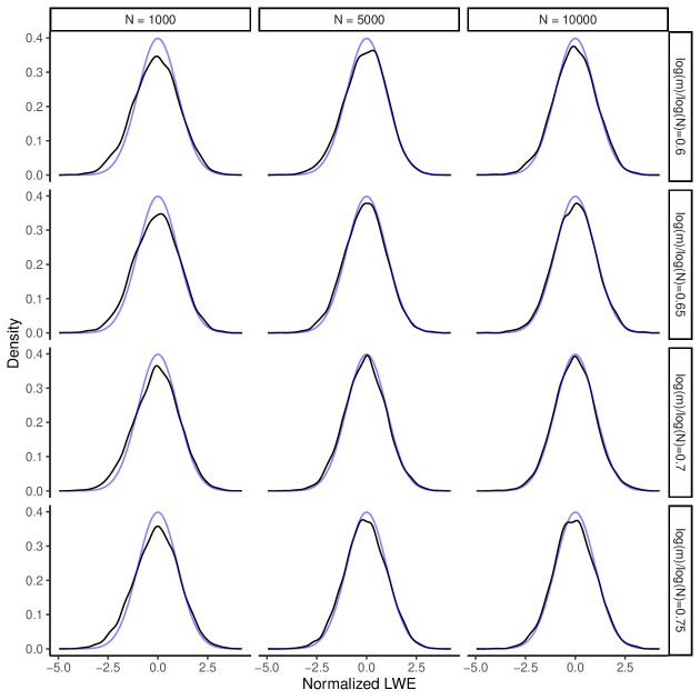
Figure 1: Empirical density functions of $T^{(R)}$ based on $5{,}000$ replications with the standard normal density overlaid in blue. The $r_{t}$ follow GARCH$(1,1)$ model with $\alpha_{0}=0.5$, $\alpha_{1}=0.2$ and $\beta_{1}=0.4$.

Table 1: Empirical size (in percent) for observations from the GARCH$(1,1)$ model, based on $5{,}000$ replications.

Nominal size			1.0				5.0				10.0
$N$		1000	5000	10000		1000	5000	10000		1000	5000	10000
		$\Delta=0.30,\theta=0.25$
$m=N^{0.60}$		0.90	1.12	1.68		4.00	5.00	6.48		7.86	9.96	11.56
$m=N^{0.65}$		0.88	1.14	1.14		3.92	4.84	5.80		7.68	9.22	10.44
$m=N^{0.70}$		0.92	1.18	1.46		3.98	5.00	5.58		7.86	9.68	9.90
$m=N^{0.75}$		0.98	1.14	1.14		4.38	5.30	5.22		8.34	9.98	10.06
		$\Delta=0.30,\theta=0.50$
$m=N^{0.60}$		0.64	0.68	0.78		3.14	3.36	4.20		6.26	6.58	8.28
$m=N^{0.65}$		0.54	0.72	0.50		3.02	3.26	3.72		5.90	6.88	7.70
$m=N^{0.70}$		0.80	0.70	0.98		3.38	3.96	4.06		6.68	7.36	7.66
$m=N^{0.75}$		0.86	0.64	0.88		3.78	3.72	3.84		7.22	7.58	8.02
		$\Delta=0.30,\theta=0.75$
$m=N^{0.60}$		0.76	1.08	1.72		3.66	5.02	5.96		7.26	10.00	11.08
$m=N^{0.65}$		0.64	1.20	1.24		3.38	4.68	5.30		7.28	9.20	10.42
$m=N^{0.70}$		0.80	1.12	1.62		3.88	4.90	5.66		7.80	9.38	10.18
$m=N^{0.75}$		0.90	0.98	1.30		4.20	4.86	5.60		8.24	9.88	10.08
		$\Delta=0.60,\theta=0.25$
$m=N^{0.60}$		1.68	1.76	1.58		6.24	6.04	6.00		11.12	11.10	11.32
$m=N^{0.65}$		1.74	1.50	1.26		6.02	6.08	6.02		10.94	10.44	10.34
$m=N^{0.70}$		1.52	1.44	1.64		5.70	6.06	6.04		10.78	11.04	10.24
$m=N^{0.75}$		1.50	1.36	1.54		6.12	5.88	5.84		11.12	11.06	10.62
		$\Delta=0.60,\theta=0.5$
$m=N^{0.60}$		0.78	0.74	0.72		3.82	3.74	4.32		7.68	7.24	8.62
$m=N^{0.65}$		0.66	0.78	0.60		3.68	3.56	4.08		7.30	7.48	8.20
$m=N^{0.70}$		0.86	0.84	1.00		3.98	4.18	4.20		7.60	7.82	8.12
$m=N^{0.75}$		0.98	0.70	0.94		4.38	4.30	4.06		8.10	8.18	8.52
		$\Delta=0.60,\theta=0.75$
$m=N^{0.60}$		1.58	1.82	1.66		6.16	6.32	6.26		10.84	11.14	11.46
$m=N^{0.65}$		1.38	1.52	1.54		5.70	5.64	5.94		10.42	10.52	10.70
$m=N^{0.70}$		1.32	1.58	1.94		5.86	6.12	5.98		10.86	10.48	10.66
$m=N^{0.75}$		1.56	1.50	1.54		5.56	5.94	6.06		10.92	11.02	11.02

Table 2: Empirical size (in percent) for observations from the SV model, based on $5{,}000$ replications.

Nominal size			1.0				5.0				10.0
$N$		1000	5000	10000		1000	5000	10000		1000	5000	10000
		$\Delta=0.30,\theta=0.25$
$m=N^{0.60}$		0.72	1.08	1.22		2.74	4.94	5.34		6.04	10.22	10.40
$m=N^{0.65}$		0.66	0.80	1.08		2.64	4.32	5.16		5.84	9.40	9.62
$m=N^{0.70}$		0.68	0.86	1.06		3.06	4.08	4.96		6.14	8.68	9.74
$m=N^{0.75}$		0.58	0.90	1.38		3.16	4.72	5.18		6.74	9.36	10.06
		$\Delta=0.30,\theta=0.50$
$m=N^{0.60}$		0.62	0.58	0.66		2.68	3.32	3.66		5.28	7.44	7.46
$m=N^{0.65}$		0.52	0.50	0.58		2.50	3.52	3.36		5.18	6.88	7.16
$m=N^{0.70}$		0.62	0.54	0.72		2.62	3.28	3.50		5.72	6.84	7.64
$m=N^{0.75}$		0.58	0.50	0.92		2.88	3.82	4.10		5.72	7.74	8.12
		$\Delta=0.30,\theta=0.75$
$m=N^{0.60}$		0.78	1.06	1.20		3.06	5.20	5.68		6.04	9.98	10.54
$m=N^{0.65}$		0.60	0.82	0.90		3.00	4.74	5.10		5.98	8.90	9.90
$m=N^{0.70}$		0.72	0.80	1.00		3.24	4.56	4.78		6.66	9.22	9.58
$m=N^{0.75}$		0.68	0.78	1.20		3.22	4.76	4.90		6.48	9.58	10.00
		$\Delta=0.60,\theta=0.25$
$m=N^{0.60}$		1.12	1.78	1.64		4.94	6.88	5.78		9.44	11.78	11.26
$m=N^{0.65}$		1.04	1.70	1.46		4.66	6.30	5.72		8.64	11.50	10.52
$m=N^{0.70}$		1.00	1.48	1.44		4.62	5.54	5.44		9.26	10.58	10.34
$m=N^{0.75}$		1.00	1.46	1.44		4.38	5.98	5.74		9.14	11.00	10.88
		$\Delta=0.60,\theta=0.5$
$m=N^{0.60}$		0.72	0.66	0.82		3.18	3.74	3.94		6.44	8.18	8.12
$m=N^{0.65}$		0.60	0.54	0.62		3.04	3.94	3.68		6.34	7.78	7.76
$m=N^{0.70}$		0.78	0.54	0.76		3.20	3.74	3.80		6.78	7.66	8.08
$m=N^{0.75}$		0.76	0.64	0.94		3.36	4.34	4.44		6.92	8.40	8.80
		$\Delta=0.60,\theta=0.75$
$m=N^{0.60}$		1.24	1.68	1.80		4.80	6.20	6.24		8.96	11.74	11.20
$m=N^{0.65}$		0.82	1.42	1.38		4.56	6.40	5.66		8.88	11.20	10.80
$m=N^{0.70}$		1.04	1.42	1.54		4.74	5.78	5.66		9.20	11.28	10.16
$m=N^{0.75}$		1.06	1.46	1.72		4.40	6.14	5.84		8.96	11.16	10.68

References

• Anderson [1971] T. W. Anderson. The Statistical Analysis of Time Series. Wiley Series in Probability and Statistics. John Wiley & Sons, Inc., 1971.
• Aue et al. [2009] A. Aue, S. Hörmann, L. Horváth, and M. Reimherr. Break detection in the covariance structure of multivariate time series models. The Annals of Statistics, 37:4046–4087, 2009.
• Baek and Pipiras [2012] C. Baek and V. Pipiras. Statistical tests for changes in mean against long-range dependence. Journal of Time Series Analysis, 33:131–151, 2012.
• Baek et al. [2024] C. Baek, P. Kokoszka, and X. Meng. Test of change point versus long-range dependence in functional time series. Journal of Time Series Analysis, 2024. Forthcoming.
• Bardsley et al. [2017] P. Bardsley, L. Horváth, P. Kokoszka, and G. Young. Change point tests in functional factor models with application to yield curves. The Econometrics Journal, 20:86–117, 2017.
• Beran et al. [2013] J. Beran, Y. Feng, S. Ghosh, and R. Kulik. Long Memory Processes. Princeton University Press, 2013.
• Berkes et al. [2006] I. Berkes, L. Horváth, P. Kokoszka, and Q-M. Shao. On discriminating between long–range dependence and changes in mean. The Annals of Statistics, 34:1140–1165, 2006.
• Berkes et al. [2013] I. Berkes, L. Horváth, and G. Rice. Weak invariance principles for sums of dependent random functions. Stochastic Processes and their Applications, 123:385–403, 2013.
• Brillinger [1969] D. R. Brillinger. Asymptotic properties of spectral estimates of second order. Biometrika, 56:375–390, 08 1969.
• Chanda [2005] K. C. Chanda. Large sample properties of spectral estimators for a class of stationary nonlinear processes. Journal of Time Series Analysis, 26:1–16, 2005.
• Dette et al. [2020] H. Dette, K. Kokot, and S. Volgushev. Testing relevant hypotheses in functional time series via self-normalization. Journal of the Royal Statistical Society Series B: Statistical Methodology, 82:629–660, 2020.
• Francq and Zakoian [2019] C. Francq and J-M. Zakoian. GARCH Models: Structure, Statistical Inference and Financial Applications. John Wiley & Sons Ltd, second edition, March 2019.
• Giraitis et al. [2012] L. Giraitis, H. Koul, and D. Surgailis. Large Sample Inference for Long Memory Processes. Imperial College Press, 2012.
• Hörmann and Kokoszka [2010a] S. Hörmann and P. Kokoszka. Weakly dependent functional data. The Annals of Statistics, 38(3):1845–1884, 2010a.
• Hörmann and Kokoszka [2010b] S. Hörmann and P. Kokoszka. Weakly dependent functional data. The Annals of Statistics, 38:1845–1884, 2010b.
• Horváth et al. [2013] L. Horváth, P. Kokoszka, and R. Reeder. Estimation of the mean of functional time series and a two sample problem. Journal of the Royal Statistical Society (B), 75:103–122, 2013.
• Horváth et al. [2014] L. Horváth, P. Kokoszka, and G. Rice. Testing stationarity of functional time series. Journal of Econometrics, 179:66–82, 2014.
• Horváth et al. [2024] L. Horváth, P. Kokoszka, and S. Lu. Variable selection based testing for parameter changes in regression with autoregressive dependence. Journal of Business and Economic Statistics, 2024. Forthcoming.
• Kokoszka et al. [2015] P. Kokoszka, H. Miao, and X. Zhang. Functional dynamic factor model for intraday price curves. Journal of Financial Econometrics, 13:456–477, 2015.
• Li et al. [2021] D. Li, P. Robinson, and H L. Shang. Local Whittle estimation of long-range dependence for functional time series. Journal of Time Series Analysis, 42:685–695, 2021.
• Liu and Wu [2010] W. Liu and W. B. Wu. Asymptotics of spectral density estimates. Econometric Theory, 26:1218–1245, 2010.
• Liu et al. [2013] W. Liu, H. Xiao, and W. Wu. Probability and moment inequalities under dependence. Statistica Sinica, 23:1257–1272, 2013.
• Phillips and Shimotsu [2004] P. Phillips and K. Shimotsu. Local Whittle estimation in nonstationary and unit root cases. The Annals of Statistics, 32:656–692, 2004.
• Robinson [1995] P. Robinson. Gaussian semiparametric estimation of long range dependence. The Annals of Statistics, 23:1630–1661, 1995.
• Robinson [2008] P. Robinson. Multiple local Whittle estimation in stationary systems. The Annals of Statistics, 36:2508–2530, 2008.
• Rosenblatt [1984] M. Rosenblatt. Asymptotic normality, strong mixing and spectral density estimates. The Annals of Probability, 12:1167–1180, 1984.
• Shao and Wu [2007] X. Shao and W. B. Wu. Asymptotic spectral theory for nonlinear time series. The Annals of Statistics, 35:1773 – 1801, 2007.
• van Delft [2019] A. van Delft. A note on quadratic forms of stationary functional time series under mild conditions. arXiv e-prints, 2019.
• van Delft [2020] A. van Delft. A note on quadratic forms of stationary functional time series under mild conditions. Stochastic Processes and their Applications, 130:4206–4251, 2020.
• Velasco [1999] C. Velasco. Gaussian semiparametric estimation of non-stationary time series. Journal of Time Series Analysis, 20:87–127, 1999.
• Wu [2005] W. B. Wu. Nonlinear system theory: Another look at dependence. Proceedings of the National Academy of Sciences, 102(40):14150–14154, September 2005.
• Wu and Mielniczuk [2010] W. B. Wu and J. Mielniczuk. A new look at measuring dependence. In Dependence in Probability and Statistics, pages 123–142. Springer Berlin Heidelberg, 2010.
• Wu and Shao [2007] W. B. Wu and X. Shao. A limit theorem for quadratic forms and its applications. Econometric Theory, 23:930–951, 2007.
• Wu and Min [2005] W.B. Wu and W. Min. On linear processes with dependent innovations. Stochastic Processes and their applications, 115:939–958, 2005.
• Zhang and Wu [2017] D. Zhang and W. Wu. Asymptotic theory for estimators of high-order statistics of stationary processes. IEEE Transactions on Information Theory, 64:4907–4922, 2017.
• Zhang [2016] X. Zhang. White noise testing and model diagnostic checking for functional time series. Journal of Econometrics, 194:76–95, 2016.
• Zhou [2013] Z. Zhou. Heteroscedasticity and autocorrelation robust structural change detection. Journal of the American Statistical Association, 108:726–740, 2013.