Two-Stage Super-Resolution Simulation Method for Three-Dimensional Flow Fields Around Buildings for Real-Time Prediction of Urban Micrometeorology
Abstract
A two-stage super-resolution simulation method is proposed for building-resolving micrometeorology simulations, which considerably reduces the computation time while maintaining accuracy. The first stage employs a convolutional neural network (CNN) to correct large-scale flows above buildings in the input of low-resolution (LR) simulation results. The second stage uses another CNN to reconstruct small-scale flows between buildings from the output of the first stage, resulting in high-resolution (HR) inferences. The CNNs are trained using HR simulation data for the second stage and their coarse-grained version for the first stage. This learning approach separates the flow scales to be inferred in each stage. The effectiveness of the proposed method was evaluated using micrometeorological simulations in an actual urban area around Tokyo Station in Japan. The super-resolution simulation successfully inferred HR atmospheric flows, reducing errors by about 50% for air temperature and 60% for wind velocity compared to the LR simulations. Furthermore, the two-stage approach allowed for localized HR inferences, reducing GPU memory usage to 12% during the training phase. The total wall-clock time for a 60-min prediction was reduced to about 9.92 min, which was approximately 3.2% (i.e., a 31-fold speedup) of the HR simulation time (309 min). The proposed method demonstrates the feasibility of real-time micrometeorology predictions in urban areas with a combination of physics-based and data-driven models.
keywords:
super-resolution , image inpainting , convolutional neural network , large eddy simulation , fast fluid dynamics , street canyon[inst1] organization=Global Scientific Information and Computing Center, Tokyo Institute of Technology, addressline=2-12-1 Ookayama, Meguro-ku, city=Tokyo, postcode=1528550, country=Japan
1 Introduction
Global urbanization suggests that various challenges in cities, such as reducing heat stress and energy consumption, will become increasingly important in the future [1]. The estimation of environmental conditions, such as wind speed and air temperature, is useful for addressing these challenges [2]. For instance, architects are incorporating knowledge of micrometeorology, such as thermal airflow responses, into building designs for more comfortable thermal environments [3, 4]. Moreover, if winds around buildings can be predicted in real time, safe drone delivery could be realized [5], which would also be cost-effective and environmentally friendly [6]. Computational Fluid Dynamics (CFD) simulations based on the laws of physics are vital tools for estimating the atmospheric state on microscales in cities [3, 7]. However, such simulations are computationally expensive due to the need for high spatial resolution, such as a few meters, to resolve buildings and streets [7, 8]. Reducing this computational burden would make CFD simulations more practical for various applications in urban areas [4, 8].
Efficient numerical methods based on physics have been proposed for urban flow fields [9]. For example, the Porous Media Model (PMM) method [10] approximates buildings as porous cubes and reduces the number of grids required for CFD simulations. The Fast Fluid Dynamics (FFD) method [11, 12] employs semi-Lagrangian and fractional step approaches and achieves larger time steps in numerical integrations. Another method [5] is based on scaling techniques and adjusts pre-computed airflows based on observations at reference points to obtain fast inference. The Multizone Model (MM) method [13, 14, 15] divides the outdoor field into zones based on building layouts and solves balance equations that are derived from conservation laws. Since the number of zones is much smaller than the number of grids used in CFD simulations, quite fast computations are realized. However, the MM method assumes a uniform atmospheric state in each zone and does not incorporate turbulence models, so it should be regarded as a mathematical model that performs simplified calculations quickly, rather than as an alternative to CFD models [14, 15]. The concept of zone division in the MM method is related to our proposed method, which will be discussed in Section 2.
Recent advances in data-driven methods, such as deep learning, are impacting various science and engineering fields and are also found in urban CFD simulations. Surrogate modeling, which replaces physics-based models with data-driven models, includes several approaches, such as reduced-order models [16, 17], graph neural networks [18], and Fourier neural operators [19]. These models predict three-dimensional (3D) airflows around buildings in a recursive manner, where the predictions for the current time step are input for the next step. On the other hand, there are also useful methods that do not conduct predictions over time. For example, using instantaneous sensor data at limited locations, a generative adversarial network (GAN) can estimate the flow field at that time [20]. Additionally, a convolutional neural network (CNN) can estimate the steady airflow around buildings from their 3D information [21]. Apart from these surrogate modelings, there are also hybrids that combine physics-based and data-driven models, with a typical example being super-resolution.
Super-resolution (SR) methods have been used not only for urban flows [22, 23, 24, 25, 26] but also for larger-scale (e.g., climate-scale) flows [27, 28, 29, 30, 31], and even beyond fluid dynamics, for condensed matter physics [32] and cosmology [33]. Originally, SR is a technique for enhancing image resolution and has been studied in computer vision. The success of neural networks (NNs) for SR [34, 35] has led to an increasing number of applications in fluid dynamics. These applications include not only simulation acceleration but also various other techniques, such as data compression, as detailed in a recent review [36].
Here, we review the acceleration of fluid simulations using SR, that is, the SR simulation method [22, 25, 26, 27, 28, 29, 30, 31, 37, 38]. This scheme consists of two phases: training and testing. In the training phase, low-resolution (LR) and high-resolution (HR) physics-based fluid simulations are performed, and the resulting pairs are used as training data. The LR and HR physics-based models may differ only in resolutions [25, 26, 28, 29, 37]; or they may also differ in the governing equations, such as using different turbulence models [38]. The LR and HR simulation results have statistical relationships through experimental configurations. For instance, they may be results based on the same initial and boundary conditions [28, 37]; or the HR simulations may be driven at the lateral boundaries by the LR simulations [25, 26, 29]. NNs are then trained to infer the HR results from the LR results as input. In the subsequent testing phase (i.e., operational phase), only the LR fluid simulations are conducted, and the results are super-resolved using the trained NNs. These HR inferences can be obtained in a short time because HR numerical integration is not required, and NN inference is usually fast.
We briefly compare the SR simulation method, which is a hybrid that combines physics-based and data-driven models, with surrogate modeling methods [e.g., 16, 17, 18, 19] that only use data-driven models. The SR simulation method uses physics-based models for time evolution, making it less susceptible to error accumulation over time [26, 29]. However, since this method requires LR physics-based simulations, the computation time for these simulations can be a bottleneck for acceleration. These points will be discussed in Sections 4.1 and 4.2. On the other hand, surrogate modeling methods perform time integration using only data-driven models, such as NNs, potentially enabling faster simulations. However, these methods tend to accumulate errors more easily due to repeated time evolution using data-driven models [e.g., 19]. Such comparisons among different methods are currently insufficient for various atmospheric flows, including urban airflows; thus, further research is needed.
SR has mainly been applied to two-dimensional (2D) flow fields in urban areas [22, 23, 24, 25, 26], but SR for 3D fields has rarely been studied. One reason for this is that the shapes of buildings, which are obstacles to urban airflows, depend on the resolution. At an LR, narrow street canyons, namely, flows between buildings, cannot be represented (see the upper-left panel in Fig. 1). Thus, when enhancing the resolution of flow fields, it is necessary to reconstruct fine-scale flows in street canyons. In other words, SR becomes a composite task that includes flow-field reconstruction, which makes NN learning difficult. This difficulty can be avoided when the focus is on 2D fields [22, 23, 24, 25, 26], such as temperature or precipitation at the bottom surface (i.e., ground or building roofs). However, in practical applications, 3D distributions of air temperature or wind speed are often required.
Our previous study [24] performed this composite-task SR for 3D flow fields around buildings using an NN that incorporates image-inpainting techniques. Here, image inpainting refers to the reconstruction of missing pixels; deep-learning-based methods have been studied in computer vision [39, 40]. Our previous study [24] obtained the LR flow fields used as input by coarse-graining HR micrometeorological simulation results. Thus, the input data were sourced from the ground-truth HR data. Although an NN trained with such input can be employed for SR simulations, the inference accuracy becomes lower [28, 37]. The reason is that during actual operation, LR simulation results are used as input, which are not based on HR data. Therefore, the feasibility of SR simulations in urban cities is currently unclear. Furthermore, most SR simulations target 2D data [22, 23, 25, 26, 27, 28, 29, 30, 31, 37], such as climate-scale precipitation distributions, and there are few applications to 3D turbulent flows, even for other fluid phenomena.
The present study demonstrates the feasibility of SR simulations in urban cities. First, in Section 2, we propose a novel two-stage SR simulation method that is suitable for 3D flow fields around buildings. To evaluate the proposed method, in Section 3, LR and HR micrometeorological simulations were separately conducted for an actual urban area around Tokyo Station in Japan. In these experiments, the LR data were not sourced from the HR data. Using these 3D data, in Section 4, we show that the proposed method can achieve about 31 times faster simulations while maintaining accuracy. Finally, the conclusions are presented in Section 5. The results of this study would not only expand the applicability of CFD simulations to various current challenges in cities but also suggest the possibility of real-time micrometeorology prediction in the future.
2 Two-stage SR simulation
This study proposes a two-stage SR simulation method, specifically designed to infer atmospheric flows around urban buildings (Fig. 1). Our previous study demonstrated that small-scale flows around buildings could be qualitatively inferred from large-scale flows above these buildings [24]. This insight indicates the effectiveness of the proposed two-stage approach. The first stage focuses on inferring large-scale flows above buildings, and the second stage aims to reconstruct small-scale flows in street canyons. This method effectively reduces the computational cost of training NNs by separating the flow scales to be inferred.
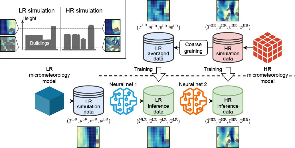
For the first stage, an NN is trained for LR inference. It is important to note that both small- and large-scale flows can differ between LR and HR micrometeorological simulations. For instance, HR simulations can represent finer-scale turbulence, which likely influences large-scale flow. In urban micrometeorology simulations, such small-scale turbulence occurs not only through spontaneous airflow evolution but also due to buildings acting as obstacles. To develop an NN for inferring such large-scale flows, we perform coarse-graining of HR simulation results, such as spatial averaging, to generate LR training data. Using these data, the NN is trained to refine the input patterns in the LR simulations without altering the resolution.
In the second stage, the LR inference from the first stage is super-resolved using another NN. This network reconstructs fine-scale flows around buildings. Training data for this stage are the results of HR simulations because such street-scale flows are simulated by the HR micrometeorology model but are not captured by the LR model (Fig. 1).
The training data, which consist of the HR simulation results and their coarse-grained versions, are required only during the training phase, not during the testing phase. In the latter actual operation, HR inference can be obtained within the computational time of LR micrometeorology simulations because the NN inference time is usually negligible. Thus, the SR simulation system shown in Fig. 1 can considerably reduce the total computational time (Section 4.2).
Another advantage of this two-stage method lies in its ability to separate inferred flow scales, thereby reducing computational costs during training. As for deep learning, more computational resources are generally needed during training because NN computational graphs must be stored on GPU memory for backpropagation, which is not necessary during testing. In the first stage, the focus is on large-scale flows; hence, detailed information on small-scale patterns is not essential. Thus, the NN can be trained with LR data, which reduces the data volume and facilitates training over more extensive spatial regions. In the second stage, modification of large-scale flows is no longer required, shifting the focus to the restoration of small-scale flows. Consequently, HR patterns can be deduced from spatially localized inputs, which means that the SR process is localized. In essence, this localization allows for training with spatially confined data and reduces the computational cost, even using HR data. The reduction in required GPU memory will be discussed in Section 4.3.
The idea behind the proposed method comes not only from our previous study [24] but also from image-inpainting studies [41, 42]. When filling in large missing regions, long-range correlations may be useful in image inpainting. To efficiently incorporate such long-range information, some image-inpainting NNs use lower-resolution images and reconstruct pixels at each resolution. The training data for these NNs consist of images at various resolutions. Consequently, these NNs can reconstruct not only the original highest-resolution image but also the images at all resolutions used. This architecture should be distinguished from those employed in ordinary U-Nets [e.g., 43]. U-Nets are designed to incorporate various scale information within the networks [44]. Rigorously speaking, however, it is not clear whether such multiple-scale information is actually utilized in the NNs without investigating their internal workings, as NN inference is generally dependent on training. The strategy in image inpainting [41, 42] enforces the learning of multiple-resolution information by employing training data at various resolutions. In our case, the NN in the first stage is forced to infer the actual LR flows due to the LR training data. This method may also be suitable for urban airflows, which are composed of various scales [2, 7].
The zone division in the MM method [13, 14, 15] may appear to be similar to the concept behind the proposed method. In particular, Yao et al. [13] divided the outdoor field into two vertical levels (i.e., upper and lower levels) and numerous horizontal zones based on the building layout. Their results suggest that such vertical division is beneficial in computing 3D flow fields in cities. In our method, a crucial difference from the MM method is that an explicit zone division is not employed. The LR inference is forced to focus on the upper large-scale flows over buildings because many street canyons are not represented due to the larger grid spacing. Furthermore, the SR simulation system can emulate fine-scale flows between buildings (Section 4.2), whereas the MM method cannot simulate such flows due to the assumption of uniformity in each zone [14, 15]. Therefore, our method is distinguished from the MM method. Mathematically, the MM method regards outdoor flow fields as graphs (i.e., nodal models) and solves the equations on these graphs. A recent study suggests that graph neural networks are effective in inferring 3D urban airflows [18]. It would be possible to further enhance SR simulations by using graph neural networks, which are considered a generalized version of CNNs [45].
3 Methods
3.1 Building-resolving micrometeorological simulations
Building-resolving micrometeorological simulations were conducted using the Multi-Scale Simulator for the Geoenvironment (MSSG) [46, 47, 48, 49]. MSSG is a coupled atmosphere-ocean model that operates on global, meso, and urban scales. The atmospheric component of MSSG, namely MSSG-A, can serve as a building-resolving large eddy simulation (LES) model in conjunction with a 3D radiative transfer model [49]. The governing equations of MSSG-A include the conservation equations of mass, momentum, and energy for compressible flows and the transport equations for the mixing ratios of water substances, such as water vapor. The results of MSSG-A were consistent with the observations under an idealized experimental setup [49]. Further information on the configurations can be found in our previous studies [22, 24, 49].
Dynamical downscaling [50] was performed for an actual urban area around Tokyo Station in Japan (35.6809∘N and 139.7670∘E) to reduce the spatio-temporal scales of atmospheric flows from meso to urban scales. The mesoscale simulations utilized three two-way-coupled [51] nested systems (Fig. 2): Domains 1 through 3. These domains are characterized by horizontal grid points of , with grid spacings of km for Domain 1, m for Domain 2, and m for Domain 3. The vertical grids for Domains 1 to 3 are identical and consist of 65 points over an altitude range of km. The initial and boundary conditions for the mesoscale simulations were obtained from the grid-point-value data of the Meso-Scale Model from the Japan Meteorological Agency [52].
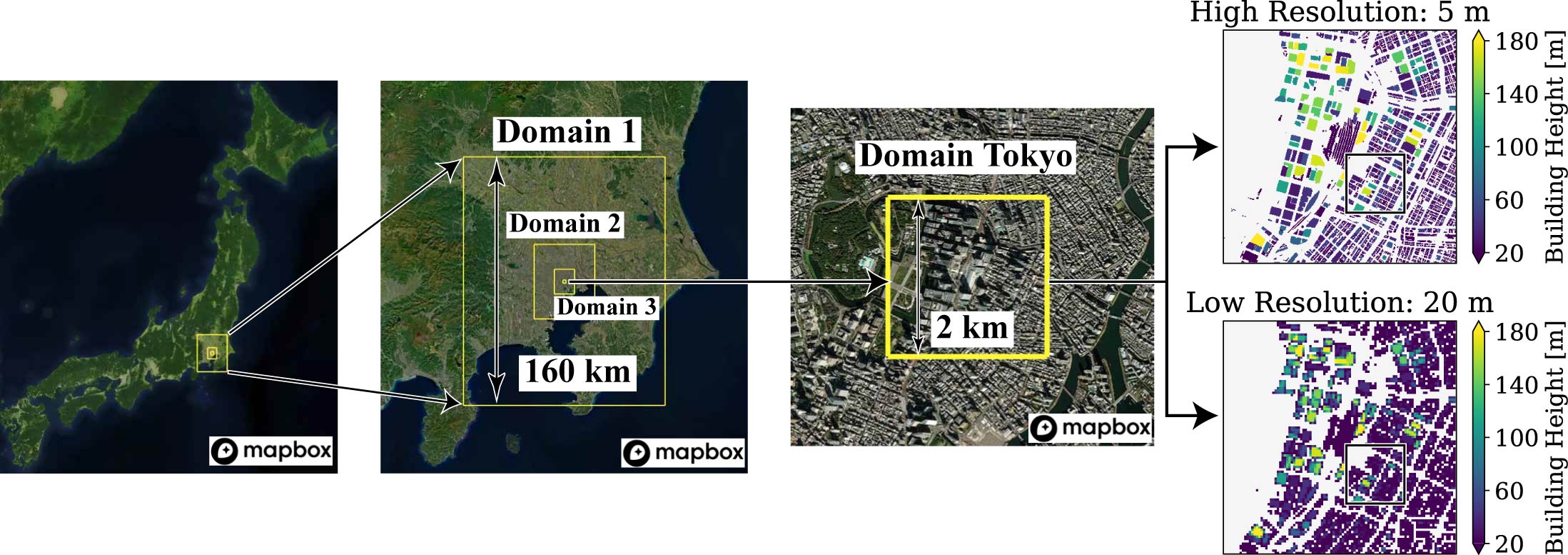
LR and HR micrometeorological simulations used a km square domain centered at Tokyo Station (i.e., Domain Tokyo), nested within Domain 3 (Fig. 2). Domain Tokyo covers an altitude range of km; for deep learning, results within a height of m were used, which are strongly influenced by buildings. The horizontal and vertical grid spacings were set at m for the LR and m for the HR. The initial and boundary conditions for both the HR and LR simulations were obtained from the mesoscale simulation results of Domain 3 (i.e., one-way nesting [51]). The same subgrid-scale (SGS) turbulence model, specifically Smagorinsky-Lilly-type parameterizations [55, 56], was applied to both the LR and HR simulations [46]. Only the HR simulations incorporated 3D radiative processes [49], which account for diabatic heating from building surfaces due to solar radiation, as well as the contrast between sunlit and shaded areas caused by buildings. The height distribution of the HR buildings was sourced from an open platform of 3D urban models [57]. The LR building height distribution was obtained through average pooling from the HR distribution. Specifically, the entire region was divided into m square blocks, and each block was replaced with the mean value. Although this operation changes the shapes of the buildings, it preserves the total volume of the buildings, ensuring that the total atmospheric volume remains unchanged. In the LR simulations, most narrow street canyons are not represented due to the coarser resolution (Fig. 2). We demonstrate that the airflows within such streets can be reconstructed by SR (Section 4.2).
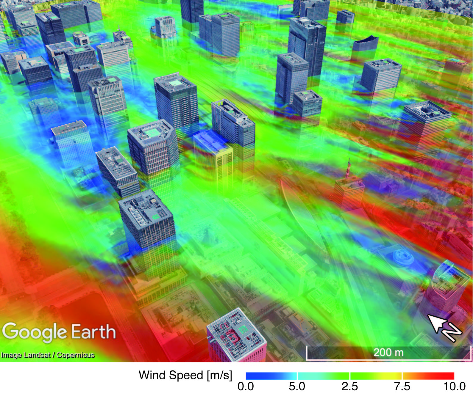
Numerical experiments were conducted for hot days between 2013 and 2020. The focus on hot days was due to the potential impact on the risk of heat-related illnesses influenced by the street-scale temperature [58]. Specifically, we selected 114 hot summer hours between 2013 and 2020, during which the maximum daily temperature exceeded 35∘C. Figure 3 shows an instantaneous snapshot of the simulated wind speed, where the airflows appear to be blocked by the buildings, and complicated turbulent flows can develop behind these buildings. Each simulation was carried out for each target hour. The results of the first 30 min were discarded to exclude a statistically non-stationary period due to the initial transient [51]; the remaining 30 min were used to obtain 1-min averaged values. The length of the initial period was determined based on the variations in temperature and velocity. We will discuss the possibility to reduce this discarded period in Section 4.3. Consequently, 30 snapshots in three dimensions were obtained from each experiment, totaling 3,420 snapshots ().
3.2 Data preparation for deep learning
We prepared training data for the two stages. The ground-truth HR data were obtained from the HR micrometeorological simulations (Section 3.1). From these simulations, the central km square area, corresponding to grid points, was extracted to eliminate the influence of the lateral damping layer on dynamical downscaling. Vertically, the bottom m region, equivalent to grid points, was extracted to focus on atmospheric flows near the ground. Four variables were used in the experiments: air temperature and the eastward, northward, and upward components of wind velocity, denoted as , , and , respectively. Each variable superscripted by is represented as a 3D numerical array with the shape of for the , , and axes, respectively. The resolution of this array is m, which means that each array covers m in the vertical direction (-axis) and m in both the north-south (-axis) and east-west (-axis) horizontal directions.
The LR ground truth for the first stage was generated by average pooling from the HR ground truth. Specifically, an HR snapshot was segmented into m cubes, and each cube was replaced with its average value. This procedure was employed to generate the LR input data in our previous study [24]. The resulting data are labeled as , , , and , where the overlines signify the averaging operation. Each variable is represented as a 3D numerical array with the shape of for the , , and axes, respectively, corresponding to a resolution of m for each axis.
The input data for the first stage were obtained from the LR micrometeorology simulations (Section 3.1). We extracted the central km square and the bottom m region, similar to the generation of the ground-truth data. The input set of , , , is distinguished from the set of , , , and . The former (without overlines) originates directly from the LR simulations, whereas the latter (with overlines) results from applying average pooling to the HR simulation outcomes. Additionally, we input a building mask , which is a binary mask derived from the LR building height distribution [24]:
| (1) |
The input data for the second stage comprise the LR output of the first stage, along with an HR building mask , which was derived from the HR building height distribution in the same manner as in Eq. (1). The input, output, and ground truth for both stages are summarized in Table 1. The term “output” refers to the inferences made by NNs, and these outputs have the same shapes as those of the corresponding ground truth.
| Stage | Kind | Variables |
|---|---|---|
| First | Ground truth | , , , |
| First | Output | |
| First | Input | |
| Second | Ground truth | |
| Second | Output | |
| Second | Input |
All pairs of the input and ground truth were split into training, validation, and test datasets at ratios of 69%, 15%, and 16%, respectively. This splitting preserves the chronological order to prevent the so-called data leakage. Specifically, the training dataset was obtained from 79 micrometeorological simulations between 2013 and 2019 (2,370 pairs); the validation set was obtained from 17 simulations in 2019 (510 pairs); and the test set was obtained from 18 in 2020 (540 pairs).
3.3 Convolutional neural networks (CNNs)
We employed two CNNs for the two-stage SR that are based on the U-Net proposed in our previous study [24]. Figure 4 shows the network architectures of the CNNs for the first and second stages, which are referred to as U-Net1 and U-Net2, respectively. U-Net1 infers LR flow fields from LR micrometeorological simulation results; then, these LR inferences from U-Net1 are super-resolved by U-Net2. Details of the U-Net1 and U-Net2 implementations are available in the Zenodo repository (see Data availability). We briefly describe the U-Net1 and U-Net2 architectures and then emphasize the differences from the CNN used in our previous study [24].
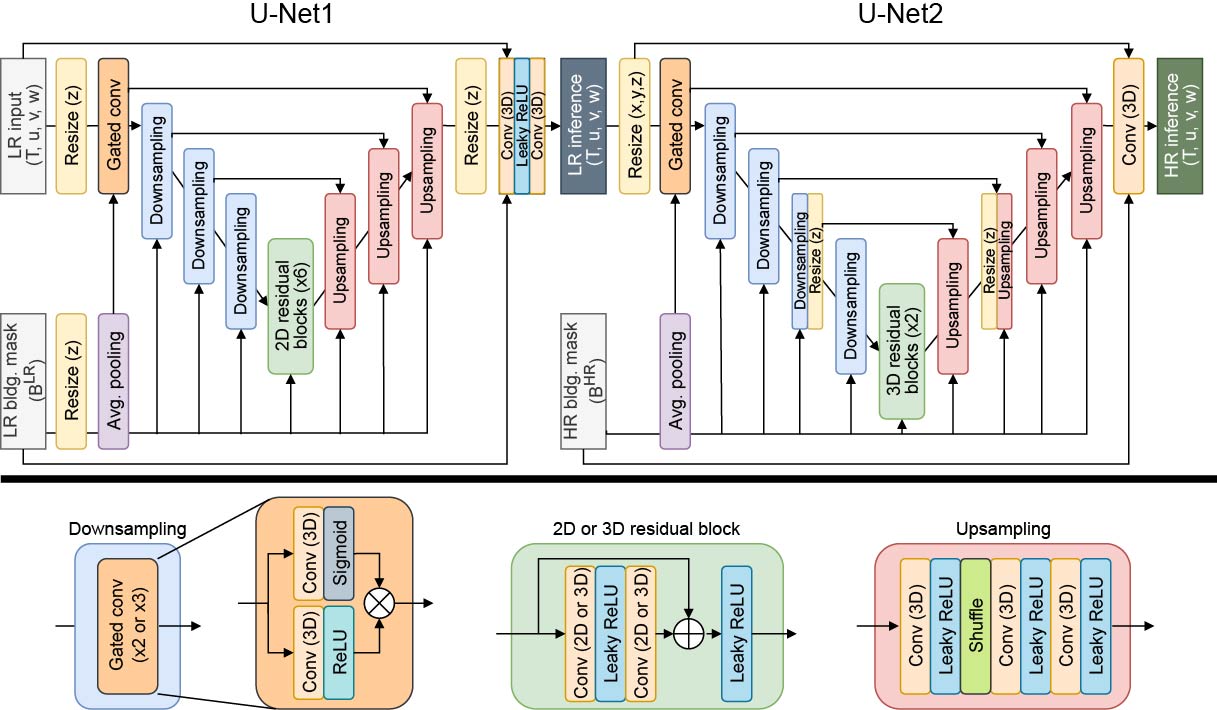
U-Net1 and U-Net2 reduce the size of the input using downsampling blocks and then restore it to its original size through upsampling blocks [44], like other U-Net type NNs [43]. This process is expected to learn features on various scales. In the downsampling step, we employ an image-inpainting technique called gated convolution [61], which is effective in reconstructing street-scale flows around buildings [24]. Specifically, the gated convolution tends to assign greater weight to non-missing values outside buildings through a sigmoid function, thereby reducing the impact of missing values (i.e., building grids) and efficiently extracting features. After downsampling, the smaller-sized data are non-linearly transformed through residual blocks [62]. Subsequently, these data are upsampled to produce output with the same size as the original. Importantly, U-Net2 initially resizes the LR input to the same size as that of HR data using nearest-neighbor interpolation, which is labeled as “Resize (x,y,z)” in Fig. 4, resulting in an HR output [24]. Both U-Net1 and U-Net2 have inputs and outputs consisting of four components: , , , and (Table 1). In addition to these inputs, the LR and HR building masks are fed into U-Net1 and U-Net2, respectively. These building masks are resized using average pooling if necessary and then fed into each block within each network. This technique is crucial for the restoration of missing values [63].
The main difference from our previous study [24] is the data size, which necessitates resizing. The repeated downsampling and upsampling require the data size to be for each direction, where is a natural number. For the horizontal directions (the and axes), resizing is not required due to the size of for the LR and for the HR (Section 3.2); however, for the vertical direction (the axis), resizing is needed due to the size of for the LR and for the HR. As for U-Net2, vertical resizing is inserted after the third downsampling block and before the second upsampling block, where these resizing blocks are labeled “Resize (z)” in Fig. 4. U-Net1 also uses such vertical resizing before downsampling and after upsampling. We confirmed that the accuracy of U-Net1 and U-Net2 is not sensitive to the locations of the resizing blocks.
More importantly, the latent space is 2D for U-Net1, whereas it is 3D for U-Net2 and the CNN in our previous study [24]. Here, the latent space refers to the feature space where non-linear transformations, labeled as residual blocks, are applied (Fig. 4). This two-dimensionality stems from the vertical size being smaller than the horizontal sizes, particularly for the LR data (). The vertical size of is reduced to by downsampling. The two-dimensionalization for LR data is consistent with the proposed two-stage SR. In this scheme, the first stage of LR inference focuses on large-scale flows above buildings, where the vertical relationship between upper and lower flows is not crucial. We treat these flow fields as 2D data within the latent space, which can lead to successful LR inferences (Section 4.1). Several studies reported that temporal information improves the SR of fluid-flow fields [26, 37, 38, 64, 65]. In the future, when addressing spatio-temporal data, such 2D latent space will become 3D space due to the time axis, allowing for the easy application of state-of-the-art techniques from video processing in computer vision [66].
The following preprocessing is applied to treat zeros as missing values [24]. Each variable (, , , or ) is transformed as follows:
| (2) |
The clipping function () limits the range of values to . The parameters and are determined such that 99.9% of values are within the range . The same values of and were used regardless of resolution. After applying Eq. (2), the Not a Number (NaN) values at the grid points inside the buildings were replaced with zeros. Owing to this preprocessing, the spatial distribution of zeros in the input represents grid points inside buildings. This evident meaning of zeros facilitates the learning of 3D image inpainting processes [24].
3.4 Training of the CNNs
The CNNs, U-Net1 and U-Net2, were trained via supervised learning, following our previous study [24]. The training method is briefly explained here.
The loss function used in training is as follows [24]:
| (3) |
where represents the ground truth, ; is the corresponding inference by the CNN; and are positive real constants; denotes mean squared quantities; represents element-wise multiplication; and signifies the second-order centered difference. The ground truth and inference are given for the first and second stages, according to Table 1. The first term in Eq. (3) evaluates the flow-field values, whereas the second and third terms quantify the differences in the flow-field smoothness and are referred to as the mean gradient error [63, 67] and the mean divergence error [38, 63], respectively. The modified building mask in Eq. (3) is different from the building mask in Eq. (1): takes values of at the grid points nearest to buildings as well as inside them, to exclude the invalidity of finite differences near building surfaces [24].
U-Net1 was initially trained, followed by the training of U-Net2. In the U-Net2 training, the inferences from the trained U-Net1 were used as input. The Adam optimizer [68] was employed for both trainings, with learning rates of for U-Net1 and for U-Net2. The same mini-batch size of was applied in the training of both U-Net1 and U-Net2. The parameters in the loss function [Eq. (3)] were set to and for U-Net1 and and for U-Net2. Each training was terminated by early stopping with a patience parameter of epochs. During the training of U-Net2, grid points were randomly cropped from HR data, and the corresponding region was extracted from the LR input. Since the number of vertical grid points is at the HR (Section 3.2), no cropping was performed in the vertical direction. This difference in cropping among directions is due to the strong influence of buildings along the vertical direction [24]. The sensitivity to the horizontal cropped size for U-Net2 will be discussed in Section 4.3. For the U-Net1 training, the full size of the data was used, and cropping was not applied in any direction due to the smaller data capacity of the LR data.
U-Net1 and U-Net2 were implemented using PyTorch 1.12.1 [69] and trained with distributed data parallel (DDP) using two NVIDIA A100 40GB PCIe GPU boards on the Earth Simulator at the Japan Agency for Marine-Earth Science and Technology (JAMSTEC). It took approximately hours to train U-Net1 and hours to train U-Net2. A single GPU was utilized for the evaluation. Details of the implementation are available in the Zenodo repository (see Data availability).
3.5 Metrics for evaluation of the CNNs
The CNN performance was evaluated using two types of metrics: pointwise accuracy and pattern consistency [24]. Similar metrics are also employed in other SR studies [34, 35]. We briefly explain here the metrics used in the present study.
The pointwise errors for temperature and velocity are defined as follows:
| (4) |
and
| (5) |
where the wind velocity vector is denoted by , quantities without hats represent the ground-truth variables, the summation is taken at a constant height over all test data, and denotes the number of grid points outside the buildings (i.e., ). Equations (4) and (5) are referred to as the error norms for temperature and velocity, respectively. These norms were applied to the LR and HR variables in the first and second stages, respectively, according to Table 1.
Pattern consistency is estimated using the mean structural similarity index measure (MSSIM) [70]. This metric is determined based on first- and second-moment quantities, such as covariance:
| MSSIM loss | ||||
| (6) |
where and . Here, and denote the mean and variance of the ground truth, respectively; and are the corresponding quantities of the inference; and represents the covariance between the ground truth and inference. The MSSIM loss, with values greater than or equal to , quantifies the similarity between the spatial patterns of the inference and the ground truth; smaller values indicate higher similarity. The MSSIM loss was computed separately for , , , and ; then, the resulting values were averaged across these four components. We confirmed that the differences in MSSIM loss among the components are sufficiently small. A detailed discussion of MSSIM can be found in previous studies [24, 70].
4 Results and discussion
4.1 Evaluation of LR inferences
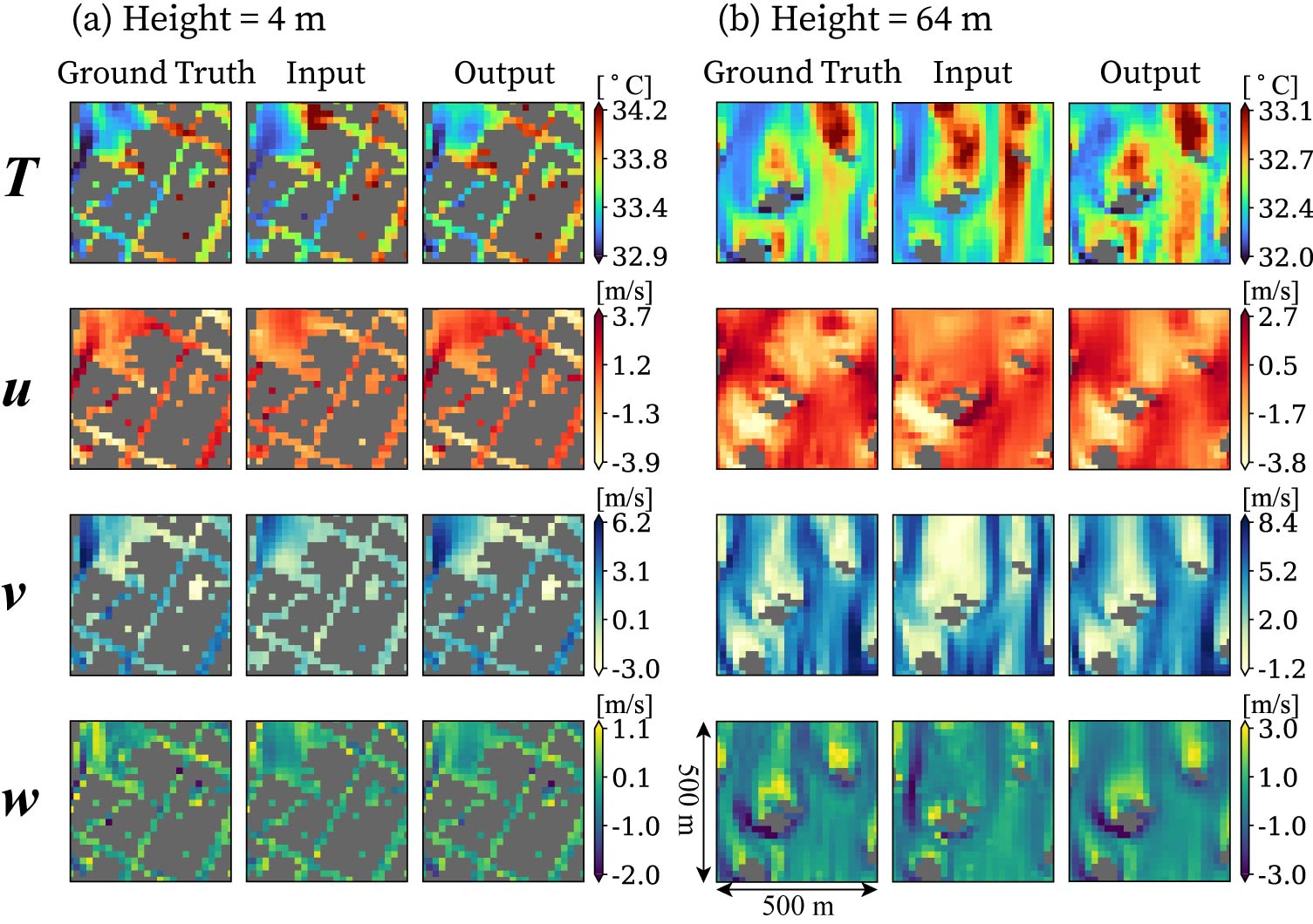
We first demonstrate the accuracy of the LR inference by the CNN, namely U-Net1. In the first stage, the ground-truth LR data are obtained by averaging the results of the HR micrometeorological simulations, whereas the input originates directly from the LR simulation results. U-Net1 modifies the flow patterns in these LR simulations to more closely resemble those of the ground truth.
Figure 5 shows an example of inference snapshots at heights of and m above the ground, where the gray areas represent missing regions due to buildings. At m, U-Net1 infers the flow pattern that blows over the street toward the vacant area in the upper left (Fig. 5a). However, the difference between the input and inference is ambiguous over the entire snapshot, as many narrow streets are not represented (i.e., missing) due to the coarse resolution. In contrast, at m, where there are fewer buildings, the differences between the input and inference become more distinct (Fig. 5b). The flows behind the buildings are considerably modified by U-Net1, becoming similar to the flow patterns in the ground truth. As discussed in Section 3.1, although the HR and LR micrometeorology simulations employ the same initial and boundary conditions, they are executed independently, which means that they do not reference each other during simulation. This independence leads to differences in the simulated flows. U-Net1 addresses these discrepancies and modifies the atmospheric flows in the LR simulations to be closer to the large-scale flows in the HR simulations.
Quantitative analysis further confirms the accuracy of U-Net1 inference. Figure 6 shows the height dependence of the test errors, averaged over all time steps. The error reduction with increasing height likely reflects the diminished influence of buildings. At all heights, the errors in the LR inference are lower than those in the LR micrometeorology simulation. In particular, at the m height, where many LR buildings are lower than this level, the temperature error reduces from to K, and the velocity error reduces from to m s-1 (i.e., both decrease by approximately half); the MSSIM loss drops from to (i.e., a decrease by approximately one-third).
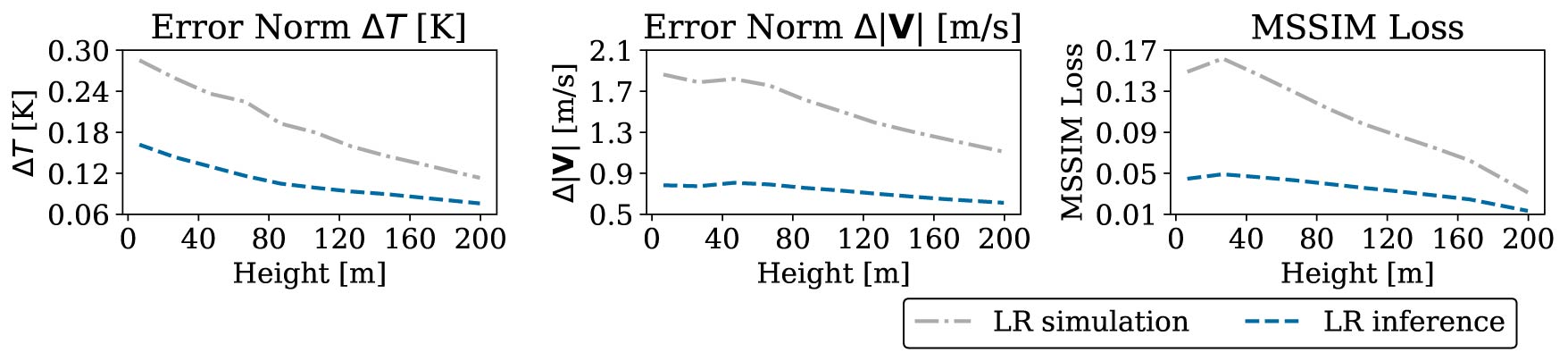
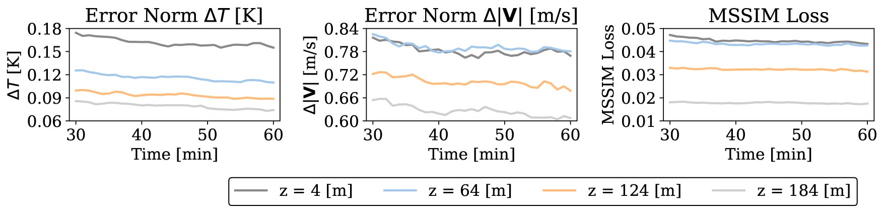
Figure 7 shows time series of the test errors for the LR inference at various heights, where averaging was performed at each time step across all the test simulations. The data from 30 to 60 min were utilized, as described in Section 3.1; hence, the time axes in the figure start at 30 min. The test errors tend to decrease with height, as discussed above (Fig. 6). The velocity error norm and MSSIM loss exhibit similar magnitudes between heights of and m, which is likely because it is more difficult to reduce error metrics based on multiple components, such as velocity vectors, as discussed in Section 4.2. Notably, the errors are nearly constant over time, with slight reductions in temperature and velocity errors. This result indicates that the inference of U-Net1 maintains high accuracy regardless of time. This point is an advantage of SR simulations (Section 1). The time evolution is computed by the LR physics-based model, not by data-driven models, which can lead to the suppression of error growth over time. Previous SR simulation studies also indicated that errors do not grow over time [26, 29], which is consistent with our result.
4.2 Evaluation of HR Inferences
Next, we demonstrate the accuracy of HR inference by the CNN, namely U-Net2. In this second stage, the ground-truth HR data are directly obtained from the HR micrometeorological simulations, while the input data consist of the LR inferences from U-Net1 in the first stage. U-Net2 reconstructs small-scale flows between buildings near the ground.
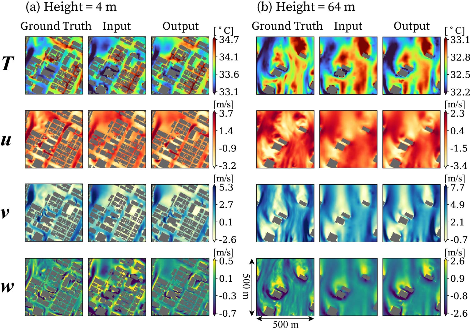
Figure 8 shows an example of inferences at heights of and m, where the gray areas represent missing regions due to buildings. The narrow streets between the buildings are depicted at a resolution of m, in contrast to the lower resolution of m. For comparison, the street-scale flows in the input shown in Fig. 8a were estimated by applying linear extrapolation to the output (i.e., the LR inference) shown in Fig. 5. At a height of m, U-Net2 successfully reconstructs the atmospheric flows in the street canyons (Fig. 8a). Specifically, in the snapshots of and , strong local winds on the streets, which are ambiguous in the input, are evident in the output. At m, the input and output, that is, the LR and HR inferences, exhibit similar patterns, as expected (Fig. 8b). These results demonstrate the effectiveness of the two-stage SR (Fig. 1): the first-stage LR inference corrects large-scale flows above buildings, and the second-stage HR inference reconstructs small-scale flows between buildings.
Quantitative analysis further confirms the accuracy of U-Net2 inference. Figure 9 compares the height dependence of the test errors among the LR micrometeorological simulation (dash-dotted lines), LR inference (dashed lines), and HR inference (solid lines). Similarly to Fig. 8, linear extrapolation was used to estimate street-scale flows in both the LR simulation and LR inference. Note that the ground truth used here is different from that in Fig. 6. In Fig. 9, we used the original HR data from the micrometeorological simulations as the ground truth, whereas in Fig. 6, their coarse-grained version was used. This distinction leads to larger errors for the LR simulation and LR inference near the ground (dash-dotted and dashed lines, respectively), compared to those in Fig. 6. Across all heights, the HR inference (solid lines) shows the smallest test errors (Fig. 9). The difference in test errors is most evident near the ground and tends to decrease with height, likely reflecting the greater impact of buildings at lower heights.
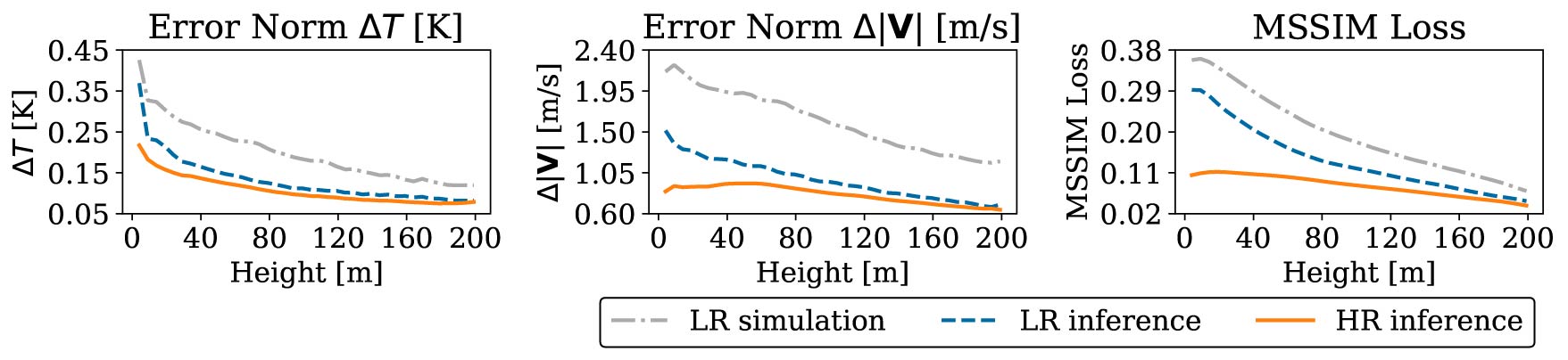
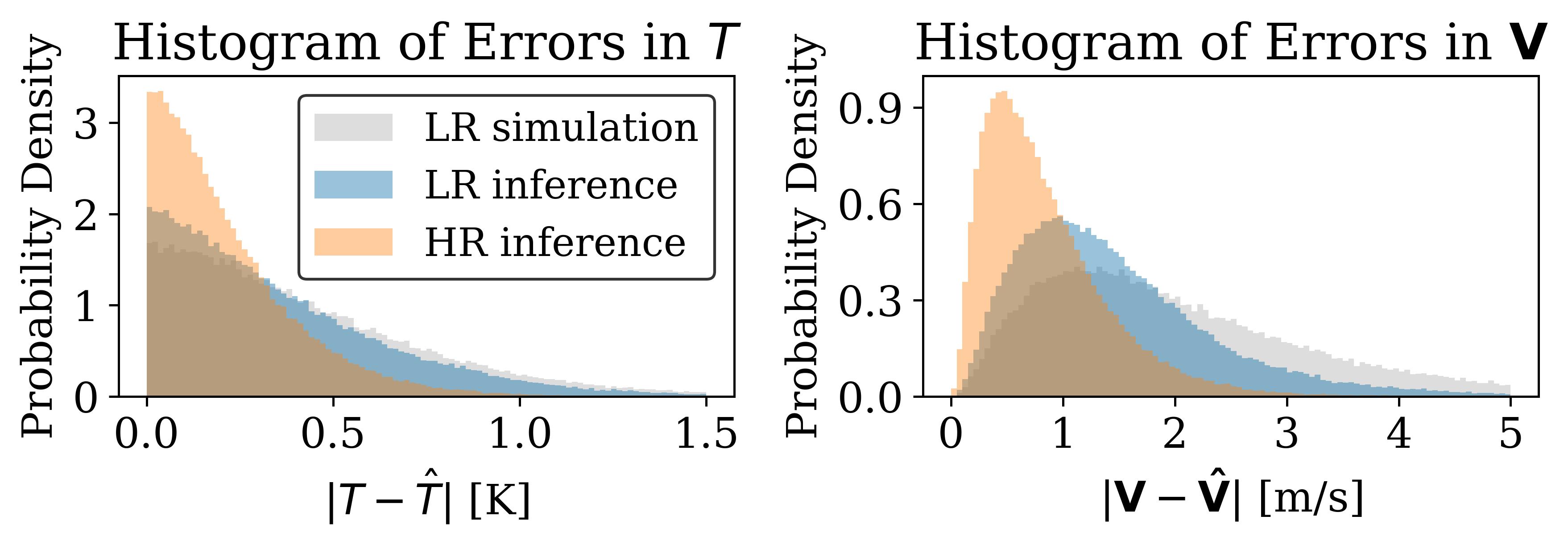
To further examine the test errors near the ground, Fig. 10 compares the histograms of pointwise errors from the LR simulation, LR inference, and HR inference at m (i.e., the lowest level). These pointwise errors are the quantities in the summations of Eqs. (4) and (5). The histogram for temperature error peaks near zero, whereas the histogram for velocity error peaks away from zero (Fig. 10). This difference in histogram shapes, also observed in our previous study [24], is likely because the temperature error is computed as the absolute difference [Eq. (4)], whereas the velocity error is based on the sum of squared differences [Eq. (5)]. This point suggests that all components of the velocity need to be reduced to decrease the velocity error norm [Eq. (5)], which likely makes the error reduction more difficult. The histograms for HR inferences are the narrowest. Indeed, not only the average values but also the th percentiles for HR inferences are equal to about 50% of those for LR simulations and 60% of those for LR inferences, as reported in Table 2. The results suggest that U-Net2 is effective in reconstructing atmospheric flows in narrow street canyons near the ground.
| Kind | Error metric | Average value | th percentile value |
|---|---|---|---|
| LR simulation | K | K | |
| LR inference | K | K | |
| HR inference | K | K | |
| LR simulation | m s-1 | m s-1 | |
| LR inference | m s-1 | m s-1 | |
| HR inference | m s-1 | m s-1 |
We report here without details that the time series of the test errors for HR inference were similar to those in Fig. 7, which indicated the nearly constant error over time. The result confirms an advantage of SR simulations again; that is, the error accumulation can be suppressed due to the time evolution by physics-based models.
Finally, we discuss the total inference time. We consider making a 60-min prediction and report wall-clock times for this prediction. The following results are based on actual measurements taken on the Earth Simulator at JAMSTEC, which employs AMD EPYC 7742 (CPUs) and NVIDIA A100 (GPUs). Specifically, HR simulations used 256 CPU cores; LR simulations used 40 CPU cores; and SR inferences used a single GPU board. On average, HR micrometeorological simulations required approximately min. Note that 90-min simulations were necessary to obtain 60-min data because the first 30 min were discarded (Section 3.1). It took around min to perform LR micrometeorology simulations. The SR process for the 60-min LR data (i.e., snapshots) totaled s, with s for the initial LR inferences and s for the subsequent HR inferences. Consequently, the SR simulation system completed a 60-min prediction in approximately min, reducing the HR computation time from min to % (i.e., a times speedup). This speedup factor is comparable with those reported in the latest surrogate modeling approaches for urban 3D flow simulations [18, 19], although direct comparisons are difficult due to the different experimental setups.
There are potentials for further reduction of computation time. In the total inference time, most of the computation time comes from the integration of the LR micrometeorology model. This point has been discussed in Section 1; that is, the computation time of LR physics-based models can be a bottleneck for acceleration. In general, a lower-resolution model would reduce computation time more. The present study uses a four-fold LR, whereas our previous study [23] implies that an eight-fold LR can be employed. The investigation of the usage of lower-resolution models is an important future task. Apart from the resolution, there is an evident potential for further reduction in computation time if the discarded initial 30 min are utilized. This point is further discussed in the next subsection (Section 4.3).
4.3 Dependence on spatial data size in training
One method to utilize the initial 30 min is to save the results and restart the numerical integration from there. Current weather forecasting operations employ a similar restarting process, together with incorporating observational data into the initial conditions to reduce prediction errors. This process is known as data assimilation [71, 72]. Recent studies have proposed combining data assimilation with SR techniques [73, 74]. To employ such a technique, reducing computation costs is required to incorporate spatio-temporal observations when training NNs [74]. Here, we demonstrate the potential to reduce the computation cost for training NNs by using the proposed two-stage SR scheme.
Generally, in the training of NNs for SR, the use of HR data requires computer resources, such as GPU memory. For instance, in supervised learning, HR data must be loaded onto the GPU memory as target data. This demands a larger size of memory, particularly for fluid simulations, because snapshots for these simulations are 3D data. In our study, the data size at the 5 m resolution is 64 times larger than at the 20 m resolution. To mitigate memory consumption, the present study implemented the two-stage SR. In the first stage of LR inference (Fig. 1), the entire flow field was provided during training to correct large-scale atmospheric flows. Due to the smaller size of the LR data, it was possible to provide data for the entire region. In the second stage of HR inference (Fig. 1), to restore fine-scale flows in street canyons, snapshots were cropped and only the localized data were supplied for training NNs, which reduces the necessary GPU memory size. If this two-stage learning is successful, the inference in the second stage requires only local patterns and is not strongly dependent on the size of the cropped data. We verify this hypothesis here.
To examine the dependence of spatial data size in the second stage, horizontal cropping was adopted from one of the following sizes during training: , , , , and . Vertical cropping was not performed in any case, as described in Section 3.4. Thus, for instance, in the case of , each HR training data has the shape of for the , , and axes. For comparison, we trained an NN that has the same architecture as U-Net2 but uses the LR simulation results as input. We refer to the SR by this NN as the single-stage SR. Compared to the second-stage SR (Fig. 1), the single-stage SR needs to correct large-scale flows and restore fine-scale flows simultaneously. Furthermore, to investigate the sensitivity of inference, we varied the pseudo-random seed used for the weight initialization [75] and conducted five sets of training for each setup. During testing, the full size of data without cropping was inputted to assess inference accuracy, as described in Section 3.4.
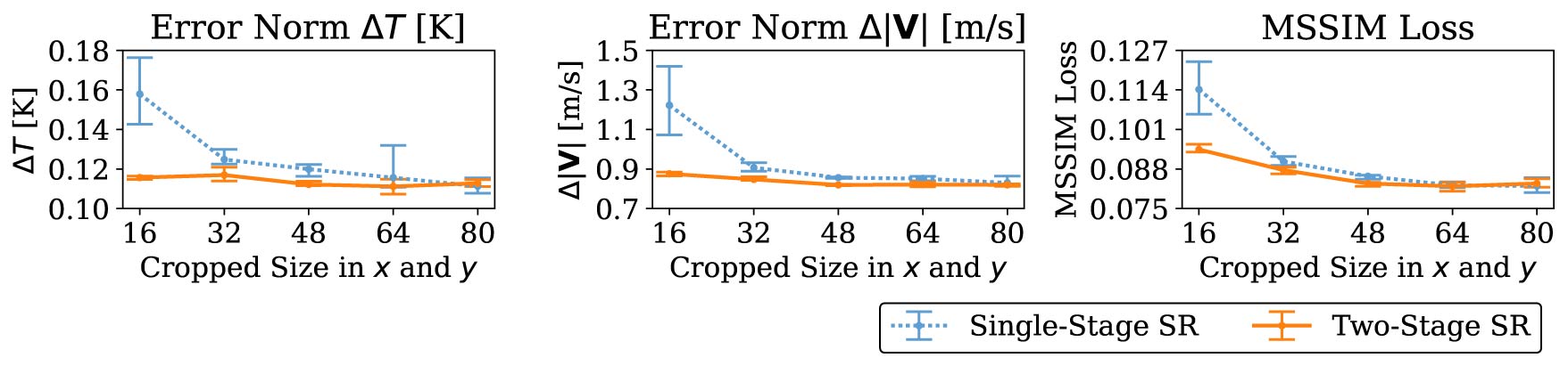
Figure 11 shows the dependence of test errors on cropped sizes. For each size, the test errors were averaged for the five U-Net2s trained using the different pseudo-random seeds; these averaged scores are represented by the lines in the figure, whereas the error bars indicate the maximum and minimum values. Compared to the single-stage SR, the two-stage SR exhibits less dependence on cropped size. In particular, the temperature and velocity error norms are nearly constant over the cropped size. The MSSIM loss tends to decrease with increasing size, while this tendency is much weaker in the two-stage SR. For the single-stage SR, all test errors decrease strongly as the size is changed from to . At the size of , the largest error suggests that U-Net2 cannot learn how to correct large-scale flows from small-size input data. When the size is equal to or greater than , the difference in accuracy between the single- and two-stage SR becomes small. This result implies that U-Net2 can learn large-scale flow correction and fine-scale flow restoration simultaneously from input data of sufficient size. Importantly, the error bars are quite large not only at but also at for the single-stage SR (see the temperature error norm in Fig. 11), suggesting that such simultaneous learning is more challenging than the separate, two-stage learning. These results indicate that the two-stage SR allows for training with smaller spatial size data, which not only localizes but also stabilizes HR inference processes.
To examine the threshold of in Fig. 11, we analyzed the histogram of city block sizes, revealing peaks around m ( grid points) and m ( grid points). These two peaks reflect that the areas to the right and left of central Tokyo station consist of smaller and larger city blocks, respectively (Fig. 2). At (80 m square), small blocks can be contained in cropped data, but larger blocks, such as 110 m squares, cannot be contained. Thus, the cropped size of likely makes it difficult to learn large-scale flow corrections, leading to the degradation in accuracy (Fig. 11). In the two-stage SR, as large-scale flow corrections are mostly addressed in the first stage, U-Net2 in the second stage only needs to reconstruct street-scale flows and can learn this reconstruction process from the cropped small-size data.
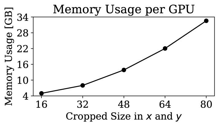
This cropping can reduce the necessary GPU memory size for the HR data. Figure 12 shows the GPU memory usage during the second-stage (i.e., U-Net2) training. Only GB are needed for size , while GB are required for size . This result indicates that the two-stage training strategy can reduce GPU memory usage even when using HR data. In our case, the proposed method can reduce memory consumption to about 12% when using the size of , compared to the case of size .
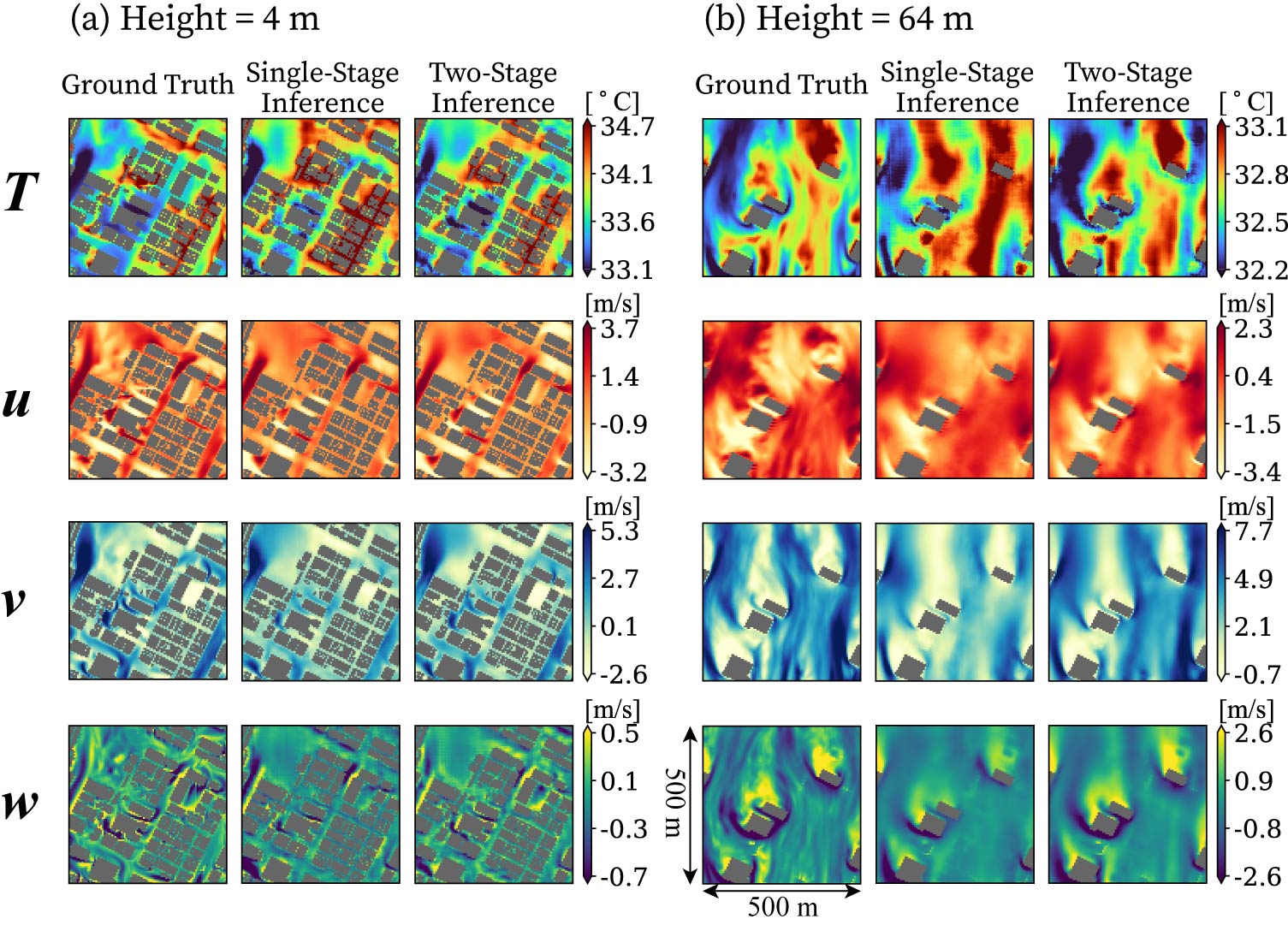
Finally, we confirm that the single-stage SR fails to learn how to correct large-scale flows when the data size is during training. Figure 13 compares snapshots of the single- and two-stage SR inference. At a height of m, both SR methods reconstruct strong local winds between buildings, although the single-stage inference slightly underestimates wind intensity. This result indicates that fine-scale flow reconstruction can be learned from spatially localized data. At m, where the flow scales are larger due to fewer buildings, the single-stage inference shows different flow patterns from those of the ground truth. In particular, the high-temperature and weak-wind areas are wider in the and snapshots, respectively. This result suggests that data of insufficient spatial size lead to the failure of learning large-scale flow corrections. In contrast, two-stage inference maintains high accuracy and yields similar patterns at m, even using small-size data (i.e., ).
5 Conclusions
This study proposed a two-stage SR simulation method suitable for building-resolving 3D fluid simulations. In this scheme, an NN corrects large-scale flows above buildings in the input of LR simulation results; then, another NN restores small-scale flows between buildings and produces the output of HR inference. The proposed method infers fine-scale flows in street canyons without HR numerical integration, thereby significantly reducing the computational cost. The proposed method facilitates the separation of flow scales targeted by inference in each stage. In particular, the second-stage inference, namely the restoration of HR flows, is spatially localized, which enables training with cropped data of a spatially smaller size. This cropping considerably reduces the GPU memory size required in deep learning.
The proposed method was evaluated by employing the building-resolving micrometeorology simulations for an actual urban area around Tokyo Station in Japan. The HR and LR simulations were conducted under the same initial and boundary conditions, whereas they did not refer to each other during numerical integration, which led to different flow patterns. The two-stage SR successfully inferred the HR flow fields from the input of the LR simulation results. Compared to the input LR simulation, the error in the HR inference was reduced by 50% for temperature and 60% for velocity. In particular, near the ground (i.e., the bottom-most level), the average errors were K for air temperature and m s-1 for wind speed. We also verified that the two-stage approach not only localizes SR processes but also stabilizes inference, compared to conventional single-stage SR. The total wall-clock time for the two-stage SR simulation was reduced to 3.21% of the original time (i.e., a 31-fold speedup), specifically from about min for HR simulations to min. These results suggest the feasibility of real-time micrometeorology prediction in urban areas.
The two-stage SR will be effective for the future integration of data assimilation, which is necessary for real-time prediction. The recent significant progress in weather forecasts using NNs is attributable to the availability of assimilated data [76, 77]. These NNs were trained using the assimilated data as a target, which is more accurate than forecast data due to the incorporation of observations. This training method is a reason why the NNs can surpass the accuracy of the current physics-based meteorology models. Unlike weather forecasts, which target atmospheric flows on kilometer or larger scales, urban micrometeorology involves airflows on meter scales and requires a lot of computational resources. This computational burden is a reason for the current absence of such assimilated data in urban areas. Recent studies have proposed combining data assimilation with SR to improve accuracy [73, 74]. Further incorporation of the present two-stage SR will not only improve accuracy but also reduce the computation cost. This future integration would develop assimilated data in urban cities and enable real-time predictions that incorporate observations through data assimilation.
Declaration of competing interest
The authors declare that they have no known competing financial interests or personal relationships that could have appeared to influence the work reported in this paper.
Data availability
The source code for deep learning is preserved at the Zenodo repository (https://doi.org/10.5281/zenodo.10903319) and developed openly at the GitHub repository (https://github.com/YukiYasuda2718/two-stage-sr-micrometeorology). The data that support the findings of this study are available from the corresponding author upon reasonable request.
Acknowledgements
The micrometeorological simulation and deep learning were performed on the Earth Simulator system (project ID: 1-23007) at the Japan Agency for Marine-Earth Science and Technology (JAMSTEC). This paper is based on results obtained from a project, JPNP22002, commissioned by the New Energy and Industrial Technology Development Organization (NEDO).
References
-
[1]
U. N. H. S. Programme, World Cities Report 2020, United Nations, 2020.
doi:10.18356/27bc31a5-en.
URL https://www.un-ilibrary.org/content/books/9789210054386 -
[2]
S. Yang, L. L. Wang, T. Stathopoulos, A. M. Marey, Urban microclimate and its impact on built environment – a review, Building and Environment 238 (2023) 110334.
doi:https://doi.org/10.1016/j.buildenv.2023.110334.
URL https://www.sciencedirect.com/science/article/pii/S036013232300361X -
[3]
C. K. C. Lam, H. Lee, S.-R. Yang, S. Park, A review on the significance and perspective of the numerical simulations of outdoor thermal environment, Sustainable Cities and Society 71 (2021) 102971.
doi:https://doi.org/10.1016/j.scs.2021.102971.
URL https://www.sciencedirect.com/science/article/pii/S2210670721002572 -
[4]
Y. Hu, Y. Peng, Z. Gao, F. Xu, Application of cfd plug-ins integrated into urban and building design platforms for performance simulations: A literature review, Frontiers of Architectural Research 12 (1) (2023) 148–174.
doi:https://doi.org/10.1016/j.foar.2022.06.005.
URL https://www.sciencedirect.com/science/article/pii/S2095263522000644 -
[5]
M. Gianfelice, H. Aboshosha, T. Ghazal, Real-time wind predictions for safe drone flights in toronto, Results in Engineering 15 (2022) 100534.
doi:https://doi.org/10.1016/j.rineng.2022.100534.
URL https://www.sciencedirect.com/science/article/pii/S2590123022002043 -
[6]
W.-C. Chiang, Y. Li, J. Shang, T. L. Urban, Impact of drone delivery on sustainability and cost: Realizing the uav potential through vehicle routing optimization, Applied Energy 242 (2019) 1164–1175.
doi:https://doi.org/10.1016/j.apenergy.2019.03.117.
URL https://www.sciencedirect.com/science/article/pii/S0306261919305252 - [7] Y. Toparlar, B. Blocken, B. Maiheu, G. J. van Heijst, A review on the cfd analysis of urban microclimate, Renewable and Sustainable Energy Reviews 80 (2017) 1613–1640. doi:10.1016/j.rser.2017.05.248.
-
[8]
P. A. Mirzaei, Cfd modeling of micro and urban climates: Problems to be solved in the new decade, Sustainable Cities and Society 69 (2021) 102839.
doi:https://doi.org/10.1016/j.scs.2021.102839.
URL https://www.sciencedirect.com/science/article/pii/S2210670721001293 -
[9]
X. Xu, Z. Gao, M. Zhang, A review of simplified numerical approaches for fast urban airflow simulation, Building and Environment 234 (2023) 110200.
doi:https://doi.org/10.1016/j.buildenv.2023.110200.
URL https://www.sciencedirect.com/science/article/pii/S0360132323002275 - [10] J. Hang, Y. Li, Wind conditions in idealized building clusters: macroscopic simulations using a porous turbulence model, Boundary-layer meteorology 136 (1) (2010) 129–159.
- [11] W. Zuo, Q. Chen, Real-time or faster-than-real-time simulation of airflow in buildings, Indoor air 19 (1) (2009) 33–44.
- [12] W. Z. Mingang Jin, Q. Chen, Simulating natural ventilation in and around buildings by fast fluid dynamics, Numerical Heat Transfer, Part A: Applications 64 (4) (2013) 273–289. doi:10.1080/10407782.2013.784131.
-
[13]
R. Yao, Q. Luo, B. Li, A simplified mathematical model for urban microclimate simulation, Building and Environment 46 (1) (2011) 253–265.
doi:https://doi.org/10.1016/j.buildenv.2010.07.019.
URL https://www.sciencedirect.com/science/article/pii/S0360132310002246 -
[14]
J. Huang, A. Zhang, R. Peng, Evaluating the multizone model for street canyon airflow in high density cities, in: Proceedings of Building Simulation 2015: 14th Conference of IBPSA, Vol. 14 of Building Simulation, IBPSA, Hyderabad, India, 2015, pp. 1032–1039.
doi:https://doi.org/10.26868/25222708.2015.2978.
URL https://publications.ibpsa.org/conference/paper/?id=bs2015_2978 -
[15]
W. Liang, J. Huang, P. Jones, Q. Wang, J. Hang, A zonal model for assessing street canyon air temperature of high-density cities, Building and Environment 132 (2018) 160–169.
doi:https://doi.org/10.1016/j.buildenv.2018.01.035.
URL https://www.sciencedirect.com/science/article/pii/S0360132318300477 -
[16]
D. Xiao, C. Heaney, L. Mottet, F. Fang, W. Lin, I. Navon, Y. Guo, O. Matar, A. Robins, C. Pain, A reduced order model for turbulent flows in the urban environment using machine learning, Building and Environment 148 (2019) 323–337.
doi:https://doi.org/10.1016/j.buildenv.2018.10.035.
URL https://www.sciencedirect.com/science/article/pii/S0360132318306607 - [17] C. E. Heaney, X. Liu, H. Go, Z. Wolffs, P. Salinas, I. M. Navon, C. C. Pain, Extending the capabilities of data-driven reduced-order models to make predictions for unseen scenarios: applied to flow around buildings, Frontiers in Physics 10 (2022) 910381.
-
[18]
X. Shao, Z. Liu, S. Zhang, Z. Zhao, C. Hu, Pignn-cfd: A physics-informed graph neural network for rapid predicting urban wind field defined on unstructured mesh, Building and Environment 232 (2023) 110056.
doi:https://doi.org/10.1016/j.buildenv.2023.110056.
URL https://www.sciencedirect.com/science/article/pii/S0360132323000835 -
[19]
W. Peng, S. Qin, S. Yang, J. Wang, X. Liu, L. L. Wang, Fourier neural operator for real-time simulation of 3d dynamic urban microclimate, Building and Environment 248 (2024) 111063.
doi:https://doi.org/10.1016/j.buildenv.2023.111063.
URL https://www.sciencedirect.com/science/article/pii/S0360132323010909 -
[20]
C. Hu, H. Kikumoto, B. Zhang, H. Jia, Fast estimation of airflow distribution in an urban model using generative adversarial networks with limited sensing data, Building and Environment 249 (2024) 111120.
doi:https://doi.org/10.1016/j.buildenv.2023.111120.
URL https://www.sciencedirect.com/science/article/pii/S0360132323011472 -
[21]
Y. Lu, X.-H. Zhou, H. Xiao, Q. Li, Using machine learning to predict urban canopy flows for land surface modeling, Geophysical Research Letters 50 (1) (2023) e2022GL102313, e2022GL102313 2022GL102313.
arXiv:https://agupubs.onlinelibrary.wiley.com/doi/pdf/10.1029/2022GL102313, doi:https://doi.org/10.1029/2022GL102313.
URL https://agupubs.onlinelibrary.wiley.com/doi/abs/10.1029/2022GL102313 - [22] R. Onishi, D. Sugiyama, K. Matsuda, Super-resolution simulation for real-time prediction of urban micrometeorology, SOLA 15 (2019) 178–182. doi:10.2151/sola.2019-032.
-
[23]
Y. Yasuda, R. Onishi, Y. Hirokawa, D. Kolomenskiy, D. Sugiyama, Super-resolution of near-surface temperature utilizing physical quantities for real-time prediction of urban micrometeorology, Building and Environment 209 (2022) 108597.
doi:https://doi.org/10.1016/j.buildenv.2021.108597.
URL https://www.sciencedirect.com/science/article/pii/S0360132321009884 -
[24]
Y. Yasuda, R. Onishi, K. Matsuda, Super-resolution of three-dimensional temperature and velocity for building-resolving urban micrometeorology using physics-guided convolutional neural networks with image inpainting techniques, Building and Environment 243 (2023) 110613.
doi:https://doi.org/10.1016/j.buildenv.2023.110613.
URL https://www.sciencedirect.com/science/article/pii/S0360132323006406 -
[25]
Y. Wu, B. Teufel, L. Sushama, S. Belair, L. Sun, Deep learning-based super-resolution climate simulator-emulator framework for urban heat studies, Geophysical Research Letters 48 (19) (2021) e2021GL094737, e2021GL094737 2021GL094737.
arXiv:https://agupubs.onlinelibrary.wiley.com/doi/pdf/10.1029/2021GL094737, doi:https://doi.org/10.1029/2021GL094737.
URL https://agupubs.onlinelibrary.wiley.com/doi/abs/10.1029/2021GL094737 -
[26]
B. Teufel, F. Carmo, L. Sushama, L. Sun, M. N. Khaliq, S. Bélair, A. Shamseldin, D. N. Kumar, J. Vaze, Physics-informed deep learning framework to model intense precipitation events at super resolution, Geoscience Letters 10 (1) (2023) 19.
doi:10.1186/s40562-023-00272-z.
URL https://doi.org/10.1186/s40562-023-00272-z - [27] E. R. Rodrigues, I. Oliveira, R. Cunha, M. Netto, Deepdownscale: A deep learning strategy for high-resolution weather forecast, 2018, pp. 415–422. doi:10.1109/eScience.2018.00130.
-
[28]
J. Wang, Z. Liu, I. Foster, W. Chang, R. Kettimuthu, V. R. Kotamarthi, Fast and accurate learned multiresolution dynamical downscaling for precipitation, Geoscientific Model Development 14 (10) (2021) 6355–6372.
doi:10.5194/gmd-14-6355-2021.
URL https://gmd.copernicus.org/articles/14/6355/2021/ -
[29]
T. T. Sekiyama, S. Hayashi, R. Kaneko, K. ichi Fukui, Surrogate downscaling of mesoscale wind fields using ensemble superresolution convolutional neural networks, Artificial Intelligence for the Earth Systems 2 (3) (2023) 230007.
doi:https://doi.org/10.1175/AIES-D-23-0007.1.
URL https://journals.ametsoc.org/view/journals/aies/2/3/AIES-D-23-0007.1.xml - [30] N. Oyama, N. N. Ishizaki, S. Koide, H. Yoshida, Deep generative model super-resolves spatially correlated multiregional climate data, Scientific Reports 13 (1) (2023) 5992.
-
[31]
J. McGibbon, S. K. Clark, B. Henn, A. Kwa, O. Watt-Meyer, W. A. Perkins, C. S. Bretherton, Global precipitation correction across a range of climates using cyclegan, Geophysical Research Letters 51 (4) (2024) e2023GL105131, e2023GL105131 2023GL105131.
arXiv:https://agupubs.onlinelibrary.wiley.com/doi/pdf/10.1029/2023GL105131, doi:https://doi.org/10.1029/2023GL105131.
URL https://agupubs.onlinelibrary.wiley.com/doi/abs/10.1029/2023GL105131 - [32] K. Shiina, H. Mori, Y. Tomita, H. K. Lee, Y. Okabe, Inverse renormalization group based on image super-resolution using deep convolutional networks, Scientific Reports 11 (12 2021). doi:10.1038/s41598-021-88605-w.
-
[33]
D. Kodi Ramanah, T. Charnock, F. Villaescusa-Navarro, B. D. Wandelt, Super-resolution emulator of cosmological simulations using deep physical models, Monthly Notices of the Royal Astronomical Society 495 (4) (2020) 4227–4236.
arXiv:https://academic.oup.com/mnras/article-pdf/495/4/4227/33372045/staa1428.pdf, doi:10.1093/mnras/staa1428.
URL https://doi.org/10.1093/mnras/staa1428 - [34] K. Chauhan, S. N. Patel, M. Kumhar, J. Bhatia, S. Tanwar, I. E. Davidson, T. F. Mazibuko, R. Sharma, Deep learning-based single-image super-resolution: A comprehensive review, IEEE Access 11 (2023) 21811–21830. doi:10.1109/ACCESS.2023.3251396.
-
[35]
D. C. Lepcha, B. Goyal, A. Dogra, V. Goyal, Image super-resolution: A comprehensive review, recent trends, challenges and applications, Information Fusion 91 (2023) 230–260.
doi:https://doi.org/10.1016/j.inffus.2022.10.007.
URL https://www.sciencedirect.com/science/article/pii/S1566253522001762 - [36] K. Fukami, K. Fukagata, K. Taira, Super-resolution analysis via machine learning: A survey for fluid flows, Theoretical and Computational Fluid Dynamics 37 (4) (2023) 421–444.
-
[37]
C. Wang, E. Bentivegna, W. Zhou, L. Klein, B. Elmegreen, Physics-informed neural network super resolution for advection-diffusion models, in: Third Workshop on Machine Learning and the Physical Sciences (NeurIPS 2020), 2020.
URL https://ml4physicalsciences.github.io/2020/ -
[38]
T. Bao, S. Chen, T. T. Johnson, P. Givi, S. Sammak, X. Jia, Physics guided neural networks for spatio-temporal super-resolution of turbulent flows, in: J. Cussens, K. Zhang (Eds.), Proceedings of the Thirty-Eighth Conference on Uncertainty in Artificial Intelligence, Vol. 180 of Proceedings of Machine Learning Research, PMLR, 2022, pp. 118–128.
URL https://proceedings.mlr.press/v180/bao22a.html - [39] O. Elharrouss, N. Almaadeed, S. Al-Maadeed, Y. Akbari, Image inpainting: A review, Neural Processing Letters 51 (2020) 2007–2028. doi:10.1007/s11063-019-10163-0.
-
[40]
Z. Qin, Q. Zeng, Y. Zong, F. Xu, Image inpainting based on deep learning: A review, Displays 69 (2021) 102028.
doi:https://doi.org/10.1016/j.displa.2021.102028.
URL https://www.sciencedirect.com/science/article/pii/S0141938221000391 - [41] M. Sharma, R. Mukhopadhyay, S. Chaudhury, B. Lall, An end-to-end deep learning framework for super-resolution based inpainting, in: R. Rameshan, C. Arora, S. Dutta Roy (Eds.), Computer Vision, Pattern Recognition, Image Processing, and Graphics, Springer Singapore, Singapore, 2018, pp. 198–208.
- [42] F. Li, A. Li, J. Qin, H. Bai, W. Lin, R. Cong, Y. Zhao, Srinpaintor: When super-resolution meets transformer for image inpainting, IEEE Transactions on Computational Imaging 8 (2022) 743–758. doi:10.1109/TCI.2022.3190142.
- [43] N. Siddique, S. Paheding, C. P. Elkin, V. Devabhaktuni, U-net and its variants for medical image segmentation: A review of theory and applications, IEEE Access 9 (2021) 82031–82057. doi:10.1109/ACCESS.2021.3086020.
- [44] O. Ronneberger, P. Fischer, T. Brox, U-net: Convolutional networks for biomedical image segmentation, in: N. Navab, J. Hornegger, W. M. Wells, A. F. Frangi (Eds.), Medical Image Computing and Computer-Assisted Intervention – MICCAI 2015, Springer International Publishing, Cham, 2015, pp. 234–241.
- [45] B. Khemani, S. Patil, K. Kotecha, S. Tanwar, A review of graph neural networks: concepts, architectures, techniques, challenges, datasets, applications, and future directions, Journal of Big Data 11 (1) (2024) 18.
-
[46]
K. Takahashi, R. Onishi, Y. Baba, S. Kida, K. Matsuda, K. Goto, H. Fuchigami, Challenge toward the prediction of typhoon behaviour and down pour, Journal of Physics: Conference Series 454 (2013) 012072.
doi:10.1088/1742-6596/454/1/012072.
URL https://iopscience.iop.org/article/10.1088/1742-6596/454/1/012072 -
[47]
R. Onishi, K. Takahashi, A warm-bin–cold-bulk hybrid cloud microphysical model*, Journal of the Atmospheric Sciences 69 (2012) 1474–1497.
doi:10.1175/JAS-D-11-0166.1.
URL https://journals.ametsoc.org/doi/10.1175/JAS-D-11-0166.1 -
[48]
W. Sasaki, R. Onishi, H. Fuchigami, K. Goto, S. Nishikawa, Y. Ishikawa, K. Takahashi, Mjo simulation in a cloud-system-resolving global ocean-atmosphere coupled model, Geophysical Research Letters 43 (2016) 9352–9360.
doi:https://doi.org/10.1002/2016GL070550.
URL https://agupubs.onlinelibrary.wiley.com/doi/abs/10.1002/2016GL070550 - [49] K. Matsuda, R. Onishi, K. Takahashi, Tree-crown-resolving large-eddy simulation coupled with three-dimensional radiative transfer model, Journal of Wind Engineering and Industrial Aerodynamics 173 (2018) 53–66. doi:10.1016/j.jweia.2017.11.015.
-
[50]
F. Giorgi, W. J. Gutowski, Regional dynamical downscaling and the cordex initiative, Annual Review of Environment and Resources 40 (1) (2015) 467–490.
arXiv:https://doi.org/10.1146/annurev-environ-102014-021217, doi:10.1146/annurev-environ-102014-021217.
URL https://doi.org/10.1146/annurev-environ-102014-021217 -
[51]
K. H. Schlünzen, D. Grawe, S. I. Bohnenstengel, I. Schlüter, R. Koppmann, Joint modelling of obstacle induced and mesoscale changes—current limits and challenges, Journal of Wind Engineering and Industrial Aerodynamics 99 (4) (2011) 217–225, the Fifth International Symposium on Computational Wind Engineering.
doi:https://doi.org/10.1016/j.jweia.2011.01.009.
URL https://www.sciencedirect.com/science/article/pii/S0167610511000110 -
[52]
Japan meteorological business support center.
URL http://www.jmbsc.or.jp/en/index-e.html -
[53]
Mapbox.
URL https://www.mapbox.com/about/maps/ -
[54]
Openstreetmap.
URL https://www.openstreetmap.org/about/ -
[55]
D. K. LILLY, On the numerical simulation of buoyant convection, Tellus 14 (2) (1962) 148–172.
arXiv:https://onlinelibrary.wiley.com/doi/pdf/10.1111/j.2153-3490.1962.tb00128.x, doi:https://doi.org/10.1111/j.2153-3490.1962.tb00128.x.
URL https://onlinelibrary.wiley.com/doi/abs/10.1111/j.2153-3490.1962.tb00128.x -
[56]
J. SMAGORINSKY, S. MANABE, J. L. HOLLOWAY, Numerical results from a nine-level general circulation model of the atmosphere1, Monthly Weather Review 93 (12) (1965) 727 – 768.
doi:10.1175/1520-0493(1965)093<0727:NRFANL>2.3.CO;2.
URL https://journals.ametsoc.org/view/journals/mwre/93/12/1520-0493_1965_093_0727_nrfanl_2_3_co_2.xml -
[57]
T. Ministry of Land, Infrastructure, Tourism, Project plateau 3d city model (2020).
URL https://www.geospatial.jp/ckan/dataset/plateau-tokyo23ku-citygml-2020 -
[58]
T. Kamiya, R. Onishi, S. Kodera, A. Hirata, Estimation of time-course core temperature and water loss in realistic adult and child models with urban micrometeorology prediction, International Journal of Environmental Research and Public Health 16 (24) (2019).
doi:10.3390/ijerph16245097.
URL https://www.mdpi.com/1660-4601/16/24/5097 -
[59]
S. Kawahara, R. Onishi, K. Goto, K. Takahashi, Realistic representation of clouds in google earth, in: SIGGRAPH Asia 2015 Visualization in High Performance Computing, SA ’15, Association for Computing Machinery, New York, NY, USA, 2015.
doi:10.1145/2818517.2818541.
URL https://doi.org/10.1145/2818517.2818541 -
[60]
W. Shi, J. Caballero, F. Huszar, J. Totz, A. P. Aitken, R. Bishop, D. Rueckert, Z. Wang, Real-time single image and video super-resolution using an efficient sub-pixel convolutional neural network, in: 2016 IEEE Conference on Computer Vision and Pattern Recognition (CVPR), IEEE Computer Society, Los Alamitos, CA, USA, 2016, pp. 1874–1883.
doi:10.1109/CVPR.2016.207.
URL https://doi.ieeecomputersociety.org/10.1109/CVPR.2016.207 - [61] J. Yu, Z. Lin, J. Yang, X. Shen, X. Lu, T. S. Huang, Free-form image inpainting with gated convolution, in: Proceedings of the IEEE/CVF International Conference on Computer Vision (ICCV), 2019.
- [62] K. He, X. Zhang, S. Ren, J. Sun, Deep residual learning for image recognition, in: Proceedings of the IEEE Conference on Computer Vision and Pattern Recognition (CVPR), 2016.
-
[63]
L. Schweri, S. Foucher, J. Tang, V. C. Azevedo, T. Günther, B. Solenthaler, A physics-aware neural network approach for flow data reconstruction from satellite observations, Frontiers in Climate 3 (2021).
doi:10.3389/fclim.2021.656505.
URL https://www.frontiersin.org/articles/10.3389/fclim.2021.656505 -
[64]
Y. Xie, E. Franz, M. Chu, N. Thuerey, Tempogan: A temporally coherent, volumetric gan for super-resolution fluid flow, ACM Trans. Graph. 37 (7 2018).
doi:10.1145/3197517.3201304.
URL https://doi.org/10.1145/3197517.3201304 -
[65]
C. Jiang, S. Esmaeilzadeh, K. Azizzadenesheli, K. Kashinath, M. Mustafa, H. A. Tchelepi, P. Marcus, M. Prabhat, A. Anandkumar, Meshfreeflownet: A physics-constrained deep continuous space-time super-resolution framework, in: 2020 SC20: International Conference for High Performance Computing, Networking, Storage and Analysis (SC), IEEE Computer Society, Los Alamitos, CA, USA, 2020, pp. 1–15.
doi:10.1109/SC41405.2020.00013.
URL https://doi.ieeecomputersociety.org/10.1109/SC41405.2020.00013 - [66] H. Liu, Z. Ruan, P. Zhao, C. Dong, F. Shang, Y. Liu, L. Yang, R. Timofte, Video super-resolution based on deep learning: a comprehensive survey, Artificial Intelligence Review 55 (8) (2022) 5981–6035.
- [67] Z. Lu, Y. Chen, Single image super-resolution based on a modified u-net with mixed gradient loss, Signal, Image and Video Processing 16 (2022) 1143–1151. doi:10.1007/s11760-021-02063-5.
-
[68]
D. P. Kingma, J. Ba, Adam: A method for stochastic optimization, 2015.
URL http://arxiv.org/abs/1412.6980 -
[69]
A. Paszke, S. Gross, F. Massa, A. Lerer, J. Bradbury, G. Chanan, T. Killeen, Z. Lin, N. Gimelshein, L. Antiga, A. Desmaison, A. Kopf, E. Yang, Z. DeVito, M. Raison, A. Tejani, S. Chilamkurthy, B. Steiner, L. Fang, J. Bai, S. Chintala, Pytorch: An imperative style, high-performance deep learning library, in: H. Wallach, H. Larochelle, A. Beygelzimer, F. d'Alché-Buc, E. Fox, R. Garnett (Eds.), Advances in Neural Information Processing Systems 32, Curran Associates, Inc., 2019, pp. 8024–8035.
URL http://papers.neurips.cc/paper/9015-pytorch-an-imperative-style-high-performance-deep-learning-library.pdf - [70] Z. Wang, A. Bovik, H. Sheikh, E. Simoncelli, Image quality assessment: from error visibility to structural similarity, IEEE Transactions on Image Processing 13 (4) (2004) 600–612. doi:10.1109/TIP.2003.819861.
-
[71]
M. Asch, M. Bocquet, M. Nodet, Data Assimilation, Society for Industrial and Applied Mathematics, Philadelphia, PA, 2016.
arXiv:https://epubs.siam.org/doi/pdf/10.1137/1.9781611974546, doi:10.1137/1.9781611974546.
URL https://epubs.siam.org/doi/abs/10.1137/1.9781611974546 -
[72]
A. Carrassi, M. Bocquet, L. Bertino, G. Evensen, Data assimilation in the geosciences: An overview of methods, issues, and perspectives, WIREs Climate Change 9 (5) (2018) e535.
arXiv:https://wires.onlinelibrary.wiley.com/doi/pdf/10.1002/wcc.535, doi:https://doi.org/10.1002/wcc.535.
URL https://wires.onlinelibrary.wiley.com/doi/abs/10.1002/wcc.535 - [73] S. Barthélémy, J. Brajard, L. Bertino, F. Counillon, Super-resolution data assimilation, Ocean Dynamics 72 (2022) 661–678. doi:10.1007/s10236-022-01523-x.
-
[74]
Y. Yasuda, R. Onishi, Spatio-temporal super-resolution data assimilation (srda) utilizing deep neural networks with domain generalization, Journal of Advances in Modeling Earth Systems 15 (11) (2023) e2023MS003658, e2023MS003658 2023MS003658.
arXiv:https://agupubs.onlinelibrary.wiley.com/doi/pdf/10.1029/2023MS003658, doi:https://doi.org/10.1029/2023MS003658.
URL https://agupubs.onlinelibrary.wiley.com/doi/abs/10.1029/2023MS003658 - [75] K. He, X. Zhang, S. Ren, J. Sun, Delving deep into rectifiers: Surpassing human-level performance on imagenet classification, in: Proceedings of the IEEE International Conference on Computer Vision (ICCV), 2015.
-
[76]
R. Lam, A. Sanchez-Gonzalez, M. Willson, P. Wirnsberger, M. Fortunato, F. Alet, S. Ravuri, T. Ewalds, Z. Eaton-Rosen, W. Hu, A. Merose, S. Hoyer, G. Holland, O. Vinyals, J. Stott, A. Pritzel, S. Mohamed, P. Battaglia, Learning skillful medium-range global weather forecasting, Science 382 (6677) (2023) 1416–1421.
arXiv:https://www.science.org/doi/pdf/10.1126/science.adi2336, doi:10.1126/science.adi2336.
URL https://www.science.org/doi/abs/10.1126/science.adi2336 - [77] K. Bi, L. Xie, H. Zhang, X. Chen, X. Gu, Q. Tian, Accurate medium-range global weather forecasting with 3d neural networks, Nature 619 (7970) (2023) 533–538.