Effector: A Python package for regional explanations

Abstract

Global feature effect methods explain a model outputting one plot per feature. The plot shows the average effect of the feature on the output, like the effect of age on the annual income. However, average effects may be misleading when derived from local effects that are heterogeneous, i.e., they significantly deviate from the average. To decrease the heterogeneity, regional effects provide multiple plots per feature, each representing the average effect within a specific subspace. For interpretability, subspaces are defined as hyperrectangles defined by a chain of logical rules, like age’s effect on annual income separately for males and females and different levels of professional experience. We introduce Effector, a Python library dedicated to regional feature effects. Effector implements well-established global effect methods, assesses the heterogeneity of each method and, based on that, provides regional effects. Effector automatically detects subspaces where regional effects have reduced heterogeneity. All global and regional effect methods share a common API, facilitating comparisons between them. Moreover, the library’s interface is extensible so new methods can be easily added and benchmarked. The library has been thoroughly tested, ships with many tutorials (https://xai-effector.github.io/) and is available under an open-source license at PyPi https://pypi.org/project/effector/ and Github https://github.com/givasile/effector.

Keywords: Explainability, interpretability, global explanations, regional explanations.

1 Introduction

The increasing adoption of machine learning (ML) in high-stakes domains like healthcare and finance has raised the demand for explainable AI (XAI) techniques (Freiesleben et al., ; Ribeiro et al., 2016). Global feature effect methods explain a black-box model through a set of plots, where each plot is the effect of a feature on the output, as in Figure 1(a).

Global effects may be misleading when the black-box model $f(\cdot)$ exhibits interactions between features. An interaction between two features, $x_{s}$ and $x_{k}$, exists when the difference in the output $f(\mathbf{x})$ as a result of changing the value of $x_{s}$ depends on the value of $x_{k}$ (Friedman and Popescu, 2008). Global effects are often computed as averages over local effects. When feature interactions are present, local effects become heterogeneous, i.e., they significantly deviate from the average (global) effect. In these cases, the global effect may be misleading, a phenomenon known as aggregation bias (Mehrabi et al., 2021; Herbinger et al., 2022).

Regional (Herbinger et al., 2023, 2022; Molnar et al., 2023; Britton, 2019; Hu et al., 2020; Scholbeck et al., 2022) or cohort explanations (Sokol and Flach, 2020), partition the input space into subspaces and compute a regional explanation within each. The partitioning aims at subspaces with homogeneous local effects, i.e., with reduced feature interactions, yielding regional effects with minimized aggregation bias (Herbinger et al., 2022). By combining these regional explanations, users can interpret the model’s behavior across the entire input space. Several libraries focus on XAI, but none targets on regional effect methods (Table 1). Therefore, we present Effector, a Python library dedicated to regional explainability methods, which:

• implements well-established global and regional effect methods, accompanied by an intuitive way to visualize the heterogeneity of each plot.

• follows a consistent and modular software design. Existing methods share a common API and novel methods can be easily added and compared to existing ones.

• demonstrates through tutorials the use of regional effects in real and synthetic datasets. Synthetic datasets we evaluate the implemented methods with ground truth.

2 Effector - A python package for global and regional feature effects

To showcase the effectiveness of Effector we use the Bike-Sharing dataset (Fanaee-T and Gama, 2014). The results are plot in Figure 1 and explained hereafter.

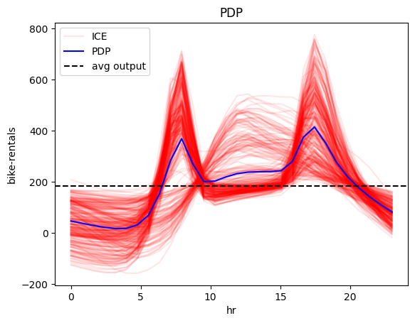
(a) Global effect

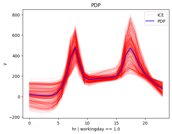
(b) Regional on weekdays

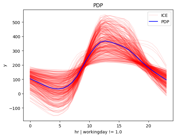
(c) Regional on weekends

Figure 1: RegionalPDP applied to the Bike Sharing dataset; Left: Global effect of feature hour on the bike-rentals. Middle: Regional effect of feature hour on weekdays. Right: Regional effect of feature hour on weekends.

Regional Effects.

Global effect methods are vulnerable to aggregation bias. Figure 1(a) shows that the global effect (blue curves) of feature hour on the bike-rentals in the Bike-Sharing dataset (Fanaee-T and Gama, 2014) has two sharp peaks at about 7:30 and 17:00 which indicate people’s commute patterns to and from work. The ICE plots (red curves), however, indicate heterogeneity; there are many instances that deviate from this explanation. Regional effect plots automatically detect two subspaces; one for weekdays (Figure 1(b)) with a peak at about 7:30 and 17:00 and one for weekends (Figure 1(c)) with a peak at about 13:00-16:00, with decreased heterogeneity compared to the global effect. The example highlights that regional effects can uncover different explanations that are hiding behind the global (average) effect.

Methods.

Figure 1 is obtained using PDP and RegionalPDP, but similar findings are obtained with any other method, as shown in Appendix D. Effector implements the following global effect methods alongside their regional counterparts; Partial Dependence Plots (PDP) (Friedman, 2001), derivative-PDP (Goldstein et al., 2014), Accumulated Local Effects (ALE) (Apley and Zhu, 2020), Robust and Heterogeneity-aware ALE (RHALE) (Gkolemis et al., 2023a) and SHAP Dependence Plots (SHAP-DP) (Lundberg and Lee, 2017). Formal descriptions of these methods are provided in Appendices A and B. Comparative analyses using synthetic examples with ground truth effects are detailed in Appendix C, while their application to real datasets is presented in Appendix D. Finally, instructions on integrating Effector with common machine learning libraries are outlined in Appendix E.

Usage.

Effector adheres to the progressive disclosure of complexity; simplifies the initial step and demands incremental learning steps for increasingly sophisticated use cases. Global or regional plots require a single-line command (lines 10 and 11 of Listing 1). In three lines of code, the user can customize the bin-splitting of RHALE (line 15) or change the heterogeneity threshold for an accepted split (line 20). All methods require two arguments: the dataset X and the predictive function f. For RHALE and d-PDP, the user can accelerate the computation, providing a function f_der that computes the derivatives with respect to the input. Otherwise, finite differences (Scholbeck et al., 2022) will be used. Effector is compatible with any underlying ML library; it only requires wrapping the trained model into a Python Callable, as shown in Appendix E.

⬇

1from effector import RHALE, RegionalRHALE

2from effector.binning_methods import DynamicProgramming

3

4# Input

5# X = .., the dataset (np.array of shape=(N,D))

6# f = .., predictive function (python callable)

7# f_der = .., predictive function’s jacobian (python callable)

8

9# 1-step global and regional effect

10RHALE(X, f, f_der).plot(feature=1)

11RegionalRHALE(x, f, f_der).plot(feature=1, node_idx=0)

12

13# 3-step global effect

14rhale = RHALE(X, f, f_der)

15rhale.fit(binning_method=DynamicProgramming(max_nof_bins=100))

16rhale.plot(feature=1)

17

18# 3-step regional effect

19regional_rhale = RegionalRHALE(X, f, f_der)

20regional_rhale.fit(heter_pcg_drop_thres=0.1)

21rhale.plot(feature=1, node_idx=0)

Listing 1: Listing showing how to use Effector.

Design

The domain of regional effects is rapidly evolving, so Effector is designed to maximize extensibility. The library is structured around a set of abstractions that facilitate the development of novel methods. For example, a user can easily experiment with a novel ALE-based approach by subclassing the ALEBase class and redefining the .fit() and .plot() methods. Or they can define a new RHALE-based heterogeneity index by subclassing the RegionalRHALE class.

Comparison to existing frameworks

Global effect methods, such as PDP and ALE, are integrated into various explainability toolkits (Pedregosa et al., 2011; Klaise et al., 2021; Baniecki et al., 2021). However, none of these toolkits implements all methods, and notably, none includes their regional counterparts, as shown in Table 1. Only DALEX offers a feature for grouping ICE plots using K-means, akin to subspace identification. As we can see, only DALEX provides functionality for grouping ICE plots using K-means, something similar to subspace detection. However, K-means clustering results in less interpretable subspaces and, notably, DALEX lacks support for the other regional effect methods.

Table 1: Comparison between current feature effect libraries and Effector

	(d-)PDP		(RH)ALE		SHAP-DP
	Global	Regional	Global	Regional	Global	Regional
InterpretML	✓	✗	✗	✗	✗	✗
DALEX	✓	$\ast$	✓	✗	✗	✗
ALIBI	✓	✗	✓	✗	✗	✗
PyALE	✗	✗	✓	✗	✗	✗
ALEPython	✗	✗	✓	✗	✗	✗
PDPbox	✓	✗	✗	✗	✗	✗
Effector	✓	✓	✓	✓	✓	✓

Broader Impact

The principle of progressive disclosure of complexity ensures Effector’s applicability in both research and industrial contexts. Users can easily get regional explanations for black-box models trained on tabular data in a single-line. Regional methods that exploit automatic differentiation, like RHALE, will be particularly useful for Deep Learning models on tabular data (Agarwal et al., 2021). Researchers can leverage Effector to develop novel methods and compare them with the existing approaches. The library will keep being updated to incorporate emerging regional effect methods.

3 Conclusion and Future Work

We introduced Effector, a Python library dedicated to regional explainability methods. The library is accessible at PyPi. Effector ships with comprehensive documentation and tutorials to familiarize the community with the realm of regional explainability methods, https://xai-effector.github.io/ Immediate plans involve accommodating multiple features of interest in the regional effect methods, as in GADGET (Herbinger et al., 2023) and to encompass other types of regional explainability methods, such as methods based on marginal effects (Scholbeck et al., 2022).

Appendix A Global Effect Methods at Effector

This section provides a brief mathematical overview of the global effect methods that are implemented at Effector. For an in-depth understanding of the methods, we refer the reader to the original papers (Friedman and Popescu, 2008; Goldstein et al., 2014; Apley and Zhu, 2020; Gkolemis et al., 2023a; Lundberg and Lee, 2017; Herbinger et al., 2023, 2022).

Each global effect method consists of a definition $f^{\texttt{m}}_{s}(x_{s})$ and an approximation $\hat{f}^{\texttt{m}}_{s}(x_{s})$, where m is the method’s name and $x_{s}$ is the feature of interest. The definition derives the effect of the $s$-th feature on the output based on the data-generating distribution $p(\mathbf{x})$ and the analytical form of the predictive function $f$. The approximation, on the other hand, estimates the effect based on the dataset instances $\mathcal{D}=\{(\mathbf{x}_{i},y_{i})\}_{i=1}^{N}$ and the predictive function $f$ treated as an input-output black-box. In real-world scenarios, only the approximation is applicable, as the data-generating distribution $p(\mathbf{x})$ and the analytical form of $f$ are unknown.

Furthermore, each method provides a way to quantify the heterogeneity of the local effects, i.e., the deviation of the local effects from the average effect. Since there is variation in how each method defines and visualizes the heterogeneity, it is difficult to provide unified mathematical notation. However, for all methods, we define a heterogeneity index $\hat{H}^{\texttt{m}}_{s}$, which quantifies the level of interactions between the $s$-th and the rest of the features and is computed using the dataset instances. This index will be later used to find the regional effects. If the method additionally provides a formal definition of the heterogeneity index using the data-generating distribution, we denote it as $H^{\texttt{m}}_{s}$. Finally, if a method also provides a way to quantify the heterogeneity at each point along the $s$-th axis, apart from a global index, we denote it as $H^{\texttt{m}}_{s}(x_{s})$ and $\hat{H}^{\texttt{m}}_{s}(x_{s})$, respectively.

For all methods, Effector implements the approximation of the global effect and the heterogeneity index for each method, which we summarize at Table 2.

Table 2: Global effect methods implemented by Effector

Method	Equation	Formula
$\hat{f}^{\mathtt{RHALE}}(x_{s})$	Eq. (4)	$\sum_{k=1}^{kx_{x_{s}}}\dfrac{z_{k}-z_{k-1}}{\left|\mathcal{S}_{k}\right|}\sum_{i:\mathbf{x}^{i}\in\mathcal{S}_{k}}\dfrac{\partial f}{\partial x_{s}}(x_{s}^{i},\mathbf{x}^{i}_{c})$
$\hat{H}^{\texttt{RHALE}}_{s}$	Eq. (6)	$\sum_{k=1}^{K_{s}}\dfrac{z_{k}-z_{k-1}}{|\mathcal{S}_{k}|}\sum_{i:\mathbf{x}^{i}\in\mathcal{S}_{k}}\left[\dfrac{\partial f}{\partial x_{s}}(x_{s}^{i},\mathbf{x}^{i}_{c})-\hat{\mu}_{k}^{\mathtt{RHALE}}\right]^{2}$
$\hat{f}^{\mathtt{ALE}}(x_{s})$	Eq. (3)	$\sum_{k=1}^{k_{x_{s}}}\dfrac{1}{|\mathcal{S}_{k}|}\sum_{i:\mathbf{x}^{i}\in\mathcal{S}_{k}}\left[f(z_{k},\mathbf{x}^{i}_{c})-f(z_{k-1},\mathbf{x}^{i}_{c})\right]$
$\hat{H}^{\texttt{ALE}}_{s}$	Eq. (5)	$\sum_{k=1}^{K}\dfrac{1}{|\mathcal{S}_{k}|}\sum_{i:\mathbf{x}^{i}\in\mathcal{S}_{k}}\left[(f(z_{k},\mathbf{x}^{i}_{c})-f(z_{k-1},\mathbf{x}^{i}_{c}))-\hat{\mu}_{k}^{\mathtt{ALE}}\right]^{2}$
$\hat{f}^{\mathtt{PDP}}(x_{s})$	Eq. (7)	$\dfrac{1}{N}\sum_{i=1}^{N}f(x_{s},\mathbf{x}^{i}_{c})$
$\hat{H}^{\texttt{PDP}}_{s}$	Eq. (8)	$\dfrac{1}{T}\sum_{t=1}^{T}\dfrac{1}{N}\sum_{i=1}^{N}\left[\hat{f}^{\mathtt{ICE}}_{i,\text{centered}}(x_{s,t})-\hat{f}_{\text{centered}}^{\mathtt{PDP}}(x_{s,t})\right]^{2}$
$\hat{f}^{\mathtt{d-PDP}}(x_{s})$	Eq. (9)	$\dfrac{1}{N}\sum_{i=1}^{N}f(x_{s},\mathbf{x}^{i}_{c})$
$\hat{H}^{\texttt{d-PDP}}_{s}$	Eq. (10)	$\dfrac{1}{T}\sum_{t=1}^{T}\dfrac{1}{N}\sum_{i=1}^{N}\left[\hat{f}^{\mathtt{ICE}}_{i,\text{centered}}(x_{s,t})-\hat{f}_{\text{centered}}^{\mathtt{PDP}}(x_{s,t})\right]^{2}$
$\hat{f}^{\mathtt{SHAP-DP}}(x_{s})$	Eq. (13)	$\kappa(x_{s}),\quad\kappa(x_{s})\text{ is a univariate spline fit to }\{(x_{s}^{i},\hat{\phi}_{s}^{i})\}_{i=1}^{N}$
$\hat{H}^{\texttt{SHAP-DP}}_{s}$	Eq. (14)	$\frac{1}{N}\sum_{i=1}^{N}\left[\hat{\phi}_{s}^{i}-f^{\mathtt{SHAP-DP}}(x_{s}^{i})\right]^{2}$

Notation.

Let $\mathcal{X}\in\mathbb{R}^{d}$ be the $d$-dimensional feature space, $\mathcal{Y}$ the target space and $f(\cdot):\mathcal{X}\rightarrow\mathcal{Y}$ the black-box function. We use index $s\in\{1,\ldots,d\}$ for the feature of interest and $/s=\{1,\ldots,d\}-s$ for the rest. For convenience, we use $(x_{s},\mathbf{x_{c}})$ to denote the input vector $(x_{1},\cdots,x_{s},\cdots,x_{D})$, $(X_{s},\mathbf{X_{c}})$ instead of $(X_{1},\cdots,X_{s},\cdots,X_{D})$ for random variables and $\mathcal{X}_{s},\mathcal{X}_{c}$ for the feature space and its complement, respectively. The training set $\mathcal{D}=\{(\mathbf{x}^{i},y^{i})\}_{i=1}^{N}$ is sampled i.i.d. from the distribution $\mathbb{P}_{X,Y}$.

A.1 ALE and RHALE

Accumulated Local Effects (ALE) was introduced by (Apley and Zhu, 2020). Subsequently, (Gkolemis et al., 2023a) introduced Robust and Heterogeneity-aware ALE (RHALE) which extends ALE’s definition with a component that quantifies the heterogeneity. Furthermore, RHALE introduced a novel approximation of both the global effect and the heterogeneity using an automated bin-splitting. ALE and RHALE can handle datasets with correlated features well, as we will illustrate below. In contrast, (d-)PDP and SHAP-DP have limitations in these cases as we will see in Sections A.2 and A.3.

ALE defines the global effect at $x_{s}$ as an accumulation of the derivative effects. The derivative effect $\mu(x_{s})$ is the expected change on the output over the conditional distribution $\mathbf{x_{c}}|x_{s}$, i.e., $\mu(x_{s})=\mathbb{E}_{\mathbf{x_{c}}|x_{s}}\left[\frac{\partial f}{\partial x_{s}}(x_{s},\mathbf{x_{c}})\right]$. ALE’s definition is:

$$f^{\mathtt{ALE}}(x_{s})=\int_{z=0}^{x_{s}}\mathbb{E}_{\mathbf{x_{c}}|x_{s}=z}\left[\frac{\partial f}{\partial x_{s}}(z,\mathbf{x_{c}})\right]\partial z$$ (1)

and is visualized with a $1D$ plot as shown in Figure 2 (Left). RHALE definition is identical to ALE, i.e., $f^{\mathtt{RHALE}}(x_{s}):=f^{\mathtt{ALE}}(x_{s})$. Additionally, RHALE quantifies the heterogeneity $H_{s}^{\mathtt{RHALE}}(x_{s})$ as the standard deviation of the derivative effects:

$$H_{s}^{\mathtt{RHALE}}(x_{s})=\sigma_{\mathbf{x_{c}}|x_{s}}\left[\frac{\partial f}{\partial x_{s}}(x_{s},\mathbf{x_{c}})\right]$$ (2)

The heterogeneity is visualized as a shaded area around the derivative effect. Therefore, RHALE’s definition proposes two separate plots; one for the average effect which is identical to ALE (Figure 2 (Left)) and another for the derivative effect along with its associated heterogeneity, i.e., $\mu(x_{s})\pm H(x_{s})$ (Figure 2 (Right)). The two plots are arranged one under the other. The heterogeneity index is the aggregated heterogeneity over the $s$-th axis, i.e., $H_{s}^{\mathtt{RHALE}}=\int_{z=0}^{x_{s}}H^{\mathtt{RHALE}}(z)\partial z$. ALE’s approximation is:

$$\hat{f}^{\mathtt{ALE}}(x_{s})=\sum_{k=1}^{k_{x_{s}}}\underbrace{\frac{1}{|\mathcal{S}_{k}|}\sum_{i:\mathbf{x}^{i}\in\mathcal{S}_{k}}\left[f(z_{k},\mathbf{x}^{i}_{c})-f(z_{k-1},\mathbf{x}^{i}_{c})\right]}_{\hat{\mu}_{k}^{\mathtt{ALE}}}$$ (3)

where $k_{x_{s}}$ the index of the bin such that $z_{k_{x-1}}\leq x_{s}<z_{k_{x}}$, $\mathcal{S}_{k}$ is the set of the instances lying at the $k$-th bin, i.e., $\mathcal{S}_{k}=\{\mathbf{x}^{i}:z_{k-1}\neq x^{(i)}_{s}<z_{k}\}$ and $\Delta x=\frac{x_{s,max}-x_{s,min}}{K}$. In ALE, the user needs to specify the number $K$ of equally-sized bins that are used to split the feature axis. RHALE resolves that by approximating the global effect as:

$$\hat{f}^{\mathtt{RHALE}}(x_{s})=\sum_{k=1}^{k_{x_{s}}}\underbrace{\frac{z_{k}-z_{k-1}}{\left|\mathcal{S}_{k}\right|}\sum_{i:\mathbf{x}^{i}\in\mathcal{S}_{k}}\frac{\partial f}{\partial x_{s}}(x_{s}^{i},\mathbf{x}^{i}_{c})}_{\hat{\mu}_{k}^{\mathtt{RHALE}}}$$ (4)

RHALE’s approximation differentiates from ALE approximation in two aspects. First, it computes the derivative effects using automatic differentiation instead of finite differences at the bin limits. This estimates the derivative effects more accurately and faster (Gkolemis et al., 2022, 2023b). Second, it automatically partitions the $s$-th axis into a sequence of $K_{s}$ variable-size intervals, i.e., $\{\mathcal{Z}_{k}\}_{k=1}^{K_{s}}$. Each interval covers a range from $z_{k-1}$ to $z_{k}$, and defines the set $\mathcal{S}_{k}$ with the instances that lie inside, i.e., $\mathcal{S}_{k}=\{x^{(i)}:z_{k-1}\leq x^{(i)}_{s}<z_{k}\}$. The automatic bin-splitting is performed by solving an optimization problem that minimizes the heterogeneity of the derivative effect within each bin (Gkolemis et al., 2023a). The approximations of the heterogeneity index is given by:

$$\hat{H}_{s}^{\mathtt{ALE}}=\sum_{k=1}^{K}\frac{1}{|\mathcal{S}_{k}|}\sum_{i:\mathbf{x}^{i}\in\mathcal{S}_{k}}\left[(f(z_{k},\mathbf{x}^{i}_{c})-f(z_{k-1},\mathbf{x}^{i}_{c}))-\hat{\mu}_{k}^{\mathtt{ALE}}\right]^{2}$$ (5)

$$\hat{H}_{s}^{\mathtt{RHALE}}=\sum_{k=1}^{K_{s}}\frac{z_{k}-z_{k-1}}{|\mathcal{S}_{k}|}\sum_{i:\mathbf{x}^{i}\in\mathcal{S}_{k}}\left[\frac{\partial f}{\partial x_{s}}(x_{s}^{i},\mathbf{x}^{i}_{c})-\hat{\mu}_{k}^{\mathtt{RHALE}}\right]^{2}$$ (6)

A.2 PDP, d-PDP, ICE, d-ICE

PDP (Friedman and Popescu, 2008) is probably the most widely used global effect method. As a way to visualize the heterogeneity, (Goldstein et al., 2014) introduced ICE plots which generate one plot per dataset instance and visualize them on top of the PDP, as shown in Figure 5(Left). Moreover, (Goldstein et al., 2014) presented d-PDP and d-ICE, the derivative counterparts of PDP and ICE, respectively. The d-PDP and d-ICE are used to visualize the derivative effect of a feature, as shown in Figure 5(Right). Both PDP and d-PDP, however, may produce misleading explanations when applied to correlated features, as we discuss below.

PDP computes the average effect of a feature by averaging the predictions over the entire dataset while holding the feature of interest constant. The PDP definition is given by $f^{\mathtt{PDP}}(x_{s})=\mathbb{E}_{\mathbf{x_{c}}}\left[f(x_{s},\mathbf{x_{c}})\right]$ and the approximation by:

$$\hat{f}^{\mathtt{PDP}}(x_{s})=\frac{1}{N}\sum_{i=1}^{N}f(x_{s},\mathbf{x}^{i}_{c})$$ (7)

The ICE plots are used on top of the PDP plot to visualize the heterogeneity of the instance-level effects. One ICE plot is defined per dataset instance, holding all features constant except of the feature of interest. The ICE plot of the $i$-th instance is given by $\hat{f}^{\mathtt{ICE}}_{i}(x_{s})=f(x_{s},\mathbf{x_{c}}^{(i)})$.

The heterogeneity index is the average squared difference between the centered-ICE, $\hat{f}^{\mathtt{ICE}}_{i,\text{centered}}(x_{s})=\hat{f}^{\mathtt{ICE}}_{i}(x_{s})-\mathbb{E}_{x_{s}}\left[\hat{f}^{\mathtt{ICE}}_{i}(x_{s})\right]$, and the centered-PDP plots, $\hat{f}_{\text{centered}}^{\mathtt{PDP}}(x_{s})=\hat{f}^{\mathtt{PDP}}(x_{s})-\mathbb{E}_{x_{s}}\left[\hat{f}^{\mathtt{PDP}}(x_{s})\right]$. The reason for centering the plots is analyzed in (Herbinger et al., 2023). The heterogeneity index is computed by splitting the $s$-th axis into a sequence of $T$ points, i.e., $\{x_{s,t}\}_{i=1}^{T}$, where $x_{s,t}=x_{s,min}+t\cdot\Delta x$ and $\Delta x=\frac{x_{s,max}-x_{s,min}}{T}$:

$$\hat{H}_{s}^{\mathtt{PDP}}=\frac{1}{T}\sum_{t=1}^{T}\frac{1}{N}\sum_{i=1}^{N}\left[\hat{f}^{\mathtt{ICE}}_{i,\text{centered}}(x_{s,t})-\hat{f}_{\text{centered}}^{\mathtt{PDP}}(x_{s,t})\right]^{2}$$ (8)

The d-PDP and d-ICE are the derivative counterparts to PDP and ICE. They calculate the derivative effect of a feature by averaging predictions across the entire dataset while keeping the feature of interest constant. The d-PDP is defined as $f^{\mathtt{d-PDP}}(x_{s})=\mathbb{E}_{\mathbf{x_{c}}}\left[\frac{\partial f}{\partial x_{s}}(x_{s},\mathbf{x_{c}})\right]$ and approximated by:

$$\hat{f}^{\mathtt{d-PDP}}(x_{s})=\frac{1}{N}\sum_{i=1}^{N}\frac{\partial f}{\partial x_{s}}(x_{s},\mathbf{x_{c}}^{(i)})$$ (9)

The d-ICE plots $\hat{f}^{\mathtt{d-ICE}}(x_{s})=\frac{\partial f}{\partial x_{s}}(x_{s},\mathbf{x_{c}}^{(i)})$ are used on top of the d-PDP plot to visualize the heterogeneity of the instance-level derivative effects. The heterogeneity index of the d-PDP is given by:

$$\hat{H}_{s}^{\mathtt{d-PDP}}=\frac{1}{T}\sum_{t=1}^{T}\frac{1}{N}\sum_{i=1}^{N}\left[\hat{f}^{\mathtt{d-ICE}}_{i}(x_{s,t})-\hat{f}^{\mathtt{d-PDP}}(x_{s,t})\right]^{2}$$ (10)

Note that the heterogeneity index for d-PDP does not require the centered plots, as the derivative effects are centered by definition. For a detailed explanation about that, we refer the reader to (Herbinger et al., 2023).

A.3 SHAP Dependence Plot

SHAP Dependence Plot (SHAP-DP) is a recent method introduced by (Lundberg and Lee, 2017). SHAP-DP builds upon SHAP values, a local explainability method used to measure the contribution of the $s$-th feature of the $i$-th instance on the output, denoted as $\phi_{s}^{i}$:

$$\phi_{s}^{i}=\frac{|Q|!(p-|Q|-1)!}{p!}\sum_{Q\subseteq\{1,\ldots,p\}\setminus\{s\}}\left(v(Q\cup s)-v(Q)\right)$$ (11)

At the core of Eq. (11) is the value of a coalition of $Q$ features, given by $v(Q)$. The value of a coalition $Q$ is the expected value of the output of the model if only the values of the features in $Q$ are known and the rest are considered unknown, i.e., $v(Q)=\mathbb{E}_{\mathbf{X}_{/Q}}\left[f(\mathbf{x}_{Q},\mathbf{X}_{/Q})\right]$. The difference $v(Q\cup\{s\})-v(Q)$ is the contribution of the $s$-th feature to the coalition $Q$. The SHAP value $\phi_{s}^{i}$ is the weighted average of the contributions over all possible coalitions $Q$, with weight $\frac{|Q|!(p-|Q|-1)!}{p!}$. The SHAP-DP is a scatter plot with the feature values on the x-axis and the SHAP values on the y-axis and i.e., $\{(x_{s}^{i},\phi_{s}^{i})\}_{i=1}^{N}$, as shown in Figure 7. For computing an average effect of the $s$-th feature, (Herbinger et al., 2023) fit a univariate spline to the dataset $\{(x_{s}^{i},\phi_{s}^{i})\}_{i=1}^{N}$, so the SHAP-DP definition is:

$$f^{\mathtt{SHAP-DP}}(x_{s})=\kappa(x_{s}),\quad\kappa(x_{s})\text{ is a univariate spline fit to }\{(x_{s}^{i},\phi_{s}^{i})\}_{i=1}^{N}$$ (12)

The number of coalitions grows exponentially with the number of features, therefore, the SHAP values are approximated using a Monte Carlo method. We denote the approximation of the SHAP values as $\hat{\phi}_{s}^{i}$. For our approximation, we use the implementation provided by the shap library. The shap library uses the exact SHAP values if the number of features is less than 10, otherwise, it uses the permutation approximation, which is a Monte Carlo sampling of coalitions. The SHAP-DP approximation is given by:

$$\hat{f}^{\mathtt{SHAP-DP}}(x_{s})=\kappa(x_{s}),\quad\kappa(x_{s})\text{ is a univariate spline fit to }\{(x_{s}^{i},\hat{\phi}_{s}^{i})\}_{i=1}^{N}$$ (13)

The heterogeneity index is the mean squared difference between the SHAP values and the SHAP-DP fit:

$$\hat{H}_{s}^{\mathtt{SHAP-DP}}=\frac{1}{N}\sum_{i=1}^{N}\left[\hat{\phi}_{s}^{i}-f^{SHAP-DP}(x_{s}^{i})\right]^{2}$$ (14)

Appendix B Regional Effect Methods

This section provides a brief overview of the regional effect methods of Effector. For a more thorough analysis, we refer the reader to (Herbinger et al., 2023). Regional effect methods yield for each individual feature $s$, a set of $T_{s}$ non-overlapping regions $\{\mathcal{R}_{st}\}_{t=1}^{T_{s}}$ where $\mathcal{R}_{st}\in\mathcal{X}_{c}$. The number of non-overlapping regions $T_{s}$ can be different for each feature, the regions $\{\mathcal{R}_{st}\}_{t=1}^{T_{s}}$ are disjoint and their union covers the entire space, i.e., $\cup_{t=1}^{T_{s}}\mathcal{R}_{st}=\mathcal{X}_{c}$. Each region $\mathcal{R}_{st}$ is associated with a regional effect $\hat{f}_{st}$ and a heterogeneity $\hat{H}_{st}$, which is computed using the dataset $\mathcal{D}_{st}$ that contains the instances of $\mathcal{D}$ that fall within $\mathcal{R}_{st}$, i.e., $\mathcal{D}_{st}=\{(\mathbf{x}^{i},y^{i}):\mathbf{x}^{i}_{c}\in\mathcal{R}_{st}\}$.

The objective is to split $\mathcal{X}_{c}$ into regions inside of which the heterogeneity is minimized:

$$\underset{\{\mathcal{R}_{st}\}_{t=1}^{T_{s}}}{\text{minimize}} \mathcal{L}_{s}=\sum_{t=1}^{T_{s}}\frac{|\mathcal{D}_{st}|}{|\mathcal{D}|}H_{st}^{\mathtt{m}}$$ (15)

subject to $$\bigcup_{t=1}^{T}\mathcal{R}_{st}=\mathcal{X}_{c}$$

$$\mathcal{R}_{st}\cap\mathcal{R}_{s\tau}=\emptyset,\quad\forall t\neq\tau$$

$H_{st}^{\mathtt{m}}$ is the heterogeneity of the $s$-th feature at region $t$, i.e., the heterogeneity computed using the dataset $\mathcal{D}_{st}$. For convenience, we denote as $H_{s0}^{\mathtt{m}}$ the heterogeneity of the $s$-th feature over the entire space $\mathcal{X}_{c}$, i.e., $H_{s0}^{\mathtt{m}}=H_{s}^{\mathtt{m}}$.The formula of $H_{st}^{\mathtt{m}}$ depends on the regional effect method. Table 2 summarizes the regional effect methods implemented by Effector.

Effector solves the optimization problem (15) using Algorithm 1. The algorithm starts with the entire space $\mathcal{X}_{c}$ and recursively splits it into two subspaces. To describe the process, imagine the following example. For feature $s=2$, the algorithm starts with $\{x_{1},x_{3}\}$ as candidate split-features for the first level of the tree. For each candidate split-feature, the algorithm determines the candidate split positions.

Since $x_{1}$ is a continuous feature, the candidate splits positions $p$ are a linearly spaced grid of $P$ points within the range of the feature, for example, $[-1,1]$, where $P$ is a hyperparameter of the algorithm. Each position splits into two subspaces, i.e., $\mathcal{R}_{s1}=\{(x_{1},x_{3}):x_{1}\leq p\}$ and $\mathcal{R}_{s2}=\{(x_{1},x_{3}):x_{1}>p\}$ and two datasets $\mathcal{D}_{s1}=\{(\mathbf{x}^{i},y^{i}):x^{i}_{1}\leq p\}$ and $\mathcal{D}_{s2}=\{(\mathbf{x}^{i},y^{i}):x^{i}_{1}>p\}$. Each split relates to a heterogeneity index which is the weighted sum of the heterogeneity of the respective subspaces, i.e., $\sum_{t=1}^{2}\frac{|\mathcal{D}_{st}|}{|\mathcal{D}|}H_{st}^{\mathtt{m}}$.

Since $x_{3}$ is a categorical feature, the candidate splits positions $p$ are the unique values of the feature, for example, $\{1,2,3\}$. Each position splits into two subspaces, i.e., $\mathcal{R}_{s1}=\{(x_{1},x_{3}):x_{3}=p\}$ and $\mathcal{R}_{s2}=\{(x_{1},x_{3}):x_{3}\neq p\}$ and two datasets $\mathcal{D}_{s1}=\{(\mathbf{x}^{i},y^{i}):x^{i}_{3}=p\}$ and $\mathcal{D}_{s2}=\{(\mathbf{x}^{i},y^{i}):x^{i}_{3}\neq p\}$. Each split relates to a heterogeneity index which is the weighted sum of the heterogeneity of the respective subspaces, i.e., $\sum_{t=1}^{2}\frac{|\mathcal{D}_{st}|}{|\mathcal{D}|}H_{st}^{\mathtt{m}}$.

The algorithm then selects the split that minimizes the heterogeneity index, which is assigned as the split of the first level of the tree, i.e. $H_{s}^{1}$. Then it continues to the next level of the tree, where it splits the subspaces of the previous level. Given the previous example, the algorithm will split the subspaces $\mathcal{R}_{s1}$ and $\mathcal{R}_{s2}$ of the first level of the tree into two subspaces each. If the weighted sum of the heterogeneity of the four subspaces reduces the heterogeneity of the previous level over the threshold $\epsilon$ (Line 8 of Algorithm 1), the algorithm will continue to the next level of the tree. If the algorithm reaches the maximum depth of the tree, it stops and returns the subspaces $\{\mathcal{R}_{st}\}_{t=1}^{2^{L}}$. The maximum tree level $L$ is a hyperparameter of the algorithm, which is proposed to be set to $L=3$ levels, i.e., a maximum of $T=2^{L}=8$ subspaces per feature.

Input : Heterogeneity function $H_{s}$, Maximum depth $L$

Output : subspaces $\{\mathcal{R}_{st}\}_{t=1}^{T_{s}}$, where $T_{s}\in\{0,2,\ldots,2^{L}\}$

$H_{s0}$ ;

  // Compute the level of interactions before any split

$D=\{(\mathbf{x}^{i},y^{i})\}_{i=1}^{N}$ ;

  // Initial dataset

$T_{s}=0$ ;

  // Initialize the number of splits for feature $s$

1 for $l=1$ to $L$ do

2       if $H_{s}^{l-1}=0$ then

             break ;

              // Stop if the heterogeneity is zero

3            

4       end if

      /* Iterate over all features $\mathbf{x_{c}}$ and candidate split positions $p$ */

       /* Find the optimal split with heterogeneity $H_{s}^{l}=\sum_{t=1}^{2^{l}}\frac{|\mathcal{D}_{st}|}{|\mathcal{D}|}H_{st}$ */

       /* Define the subspaces $\{\mathcal{R}_{st}\}_{t=1}^{2^{l}}$ and the datasets $\{\mathcal{D}_{st}\}_{t=1}^{2^{l}}$ */

5      

6      if $\frac{H_{s}^{l}}{H_{s}^{l-1}}<\epsilon$ then

             break ;

              // Stop, if heterogeneity drop is small ($<\epsilon$)

7            

8       end if

      $T_{s}=2^{l}$ ;

        // Update the number of splits for feature $s$

9      

10 end for

return $\left\{\mathcal{R}_{st}|s\in\left\{1,\ldots,D\right\},t\in\left\{1,\ldots,T_{s}\right\}\right\}$

Algorithm 1 Detectsubspaces

Algorithm 1 is a general algorithm that can be used for any regional effect method; the only thing that changes between the methods is the heterogeneity index $H_{st}^{\mathtt{m}}$.

Appendix C Synthetic Examples

In this section, we demonstrate the utilization of Effector through synthetic examples. The synthetic examples, where both the data-generating distribution $p(\mathbf{x})$ and the predictive function $f$ are known, are suitable to understand the strengths and limitations of each global and regional effect method.

Synthetic examples offer many advantages. First, they enable the computation of the global and regional effects of each method based on their definition. Consequently, the strengths and weaknesses are clear, unaffected by potential misconceptions introduced by approximation errors. Second, it is feasible to compare different approximations against a known ground truth. For example, we can objectively compare the ALE approximation versus the RHALE approximation using the ALE definition as the ground truth. Finally, comparing with a known-ground truth also serves as a sanity check for the implementations; if the approximation is close to the definition, then the implementation is correct.

C.1 Global Effect: Comparative study of Effector’s methods

This example shows how to use Effector for generating global effect plots and assessing their heterogeneity. Effector’s plots are derived from the approximation formula of each global effect method. All plots are compared with their ground-truth, which is derived from the definition of each method after applying analytical derivations.

C.1.1 Problem set-up

The data generating distribution is defined as follows: $X_{1}\sim p(x_{1})=\frac{5}{6}\mathcal{U}(x_{1};-0.5,0)+\frac{1}{6}\mathcal{U}(x_{1};0,0.5)$, $X_{2}\sim p(x_{2})=\mathcal{N}(x_{2};\mu=0,\sigma=2)$ and $x_{3}=x_{1}+\epsilon$, where $\epsilon$ is sampled from $\mathcal{N}(0,\sigma=0.1)$. Essentially, this indicates that $X_{1}$ lies within the range $[-0.5,0.5]$ with the $\frac{5}{6}$ of the samples falling in the first half $[-0.5,0]$. $X_{2}$ is independent and normally distributed around around zero ($\mu_{2}=0$, $\sigma_{2}=2$), while $X_{3}$ is highly correlated with $X_{1}$. The ‘black-box’ function is $f(x)=\sin(2\pi x_{1})(\mathbf{1}_{x_{1}<0}-2\mathbf{1}_{x_{3}<0})+x_{1}x_{2}+x_{2}$.

C.1.2 ALE and RHALE

Definition on the synthetic example.

In the synthetic example, the ALE and RHALE average effect for feature $x_{1}$ is given by:

$$f^{\mathtt{ALE}}(x_{1})=f^{\mathtt{RHALE}}(x_{1}) =\int_{z=0}^{x_{s}}\mathbb{E}_{x_{2},x_{3}|x_{1}=z}\left[\frac{\partial f}{\partial x_{1}}(z,x_{2},x_{3})\right]\partial z$$ (16)

$$=\int_{z=0}^{x_{s}}\mathbb{E}_{x_{2}}\mathbb{E}_{x_{3}|z}\left[2\pi\cos(2\pi z)(\mathbf{1}_{z<0}-2\mathbf{1}_{x_{3}<0})+x_{2}\right]\partial z$$ (17)

$$\approx\int_{z=0}^{x_{s}}-2\pi\cos(2\pi z)\mathbf{1}_{z<0}$$ (18)

$$\approx\sin(2\pi x_{1})\mathbf{1}_{x_{1}<0}$$ (19)

The result is shown in Figure 2(Left). Furthermore, RHALE visualizes the heterogeneity as $\mu(x_{1})\pm H_{1}^{\mathtt{RHALE}}(x_{1})$, where $\mu(x_{1})$ is the derivative effect and $H_{1}^{\mathtt{RHALE}}(x_{1})$ is the heterogeneity. These are given by:

$$\mu(x_{1}) =\mathbb{E}_{x_{2},x_{3}|x_{1}}\left[\frac{\partial f}{\partial x_{1}}(x_{1},x_{2},x_{3})\right]$$ (20)

$$=-2\pi\cos(2\pi x_{1})\mathbf{1}_{x_{1}<0}$$ (21)

$$H_{1}^{\mathtt{RHALE}}(x_{1}) =\sigma_{x_{2},x_{3}|x_{1}}\left[\frac{\partial f}{\partial x_{1}}(x_{1},x_{2},x_{3})\right]$$ (22)

$$=\sigma_{x_{2},x_{3}|x_{1}}\left[2\pi\cos(2\pi x_{1})(\mathbf{1}_{x_{1}<0}-2\mathbf{1}_{x_{3}<0})+x_{2}\right]$$ (23)

$$=\sigma_{2}=2$$ (24)

The heterogeneity informs that the instance-level effects are deviating from the average derivative-effect by $\pm 2$, as shown in Figure 2.

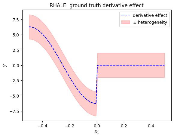
Figure 2: Left: ALE and RHALE global effect for feature $x_{1}$ based on their definitions. Right: RHALE derivative effect $\mu(x_{1})$ and its heterogeneity $H_{1}^{\mathtt{RHALE}}(x_{1})$ visualized as $\mu(x_{1})\pm H_{1}^{\mathtt{RHALE}}(x_{1})$.

Approximation using Effector.

Listing 2 shows how to use Effector to approximate the ALE effect for feature $x_{1}$ using $K$ bins. The results are shown in Figure 3; at the left figure we observe the ALE effect with 5 bins, and in the right figure, we observe the ALE effect with 20 bins. At the top of the figures, we observe the global effect, and at the bottom, the derivative effect along with the heterogeneity visualized with vertical red bars. We should observe that both $K=5$ and $K=20$ bins lead to weak approximations of the ALE effect. This is because ALE’s approximation is sensitive to the choice of $K$ and in specific cases, no fixed-size binning can provide a good approximation of the ALE effect.

⬇

1from effector.binning_methods import Fixed

2from effector import ALE

3

4# input

5# x = .., the dataset (np.array of shape=(N,D))

6# f = .., predictive function (python callable)

7

8# ALE

9ale = effector.ALE(data=x, model=f)

10for k in [5, 20]:

11 binning_method = binning_methods.Fixed(nof_bins=K)

12 ale.fit(feat, binning_method=binning_method)

13 ale.plot(feature=0, heterogeneity=True, centering=True)

Listing 2: Listing with how to use Effector to approximate the ALE effect for the first feature using $K$ bins.

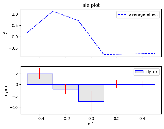
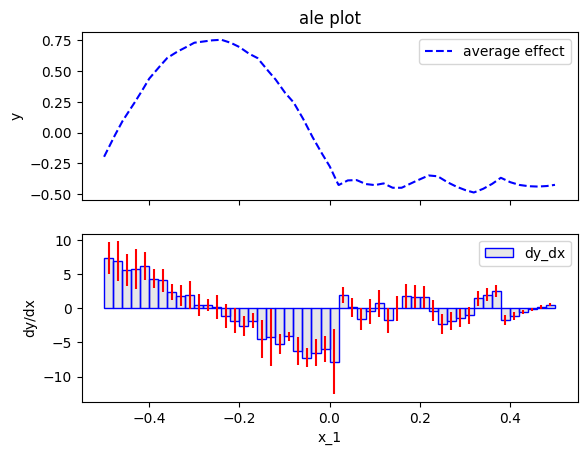
Figure 3: ALE effect for feature $x_{1}$ using 5 (left) and 20 bins (right).

In Listing 3, we show how to use Effector to approximate the RHALE effect for feature $x_{1}$ using DynamicProgramming and Greedy optimization. As stated above, RHALE automatically splits the $s$-th feature into variable-size bins. The automatic bin-splitting is performed by solving an optimization problem that minimizes the heterogeneity of the derivative effect within each bin. For an in-depth explanation of the optimization problem, we refer the reader to (Gkolemis et al., 2023a). The optimization problem can be solved either using DynamicProgramming, which ensures a globally optimal solution, or with a Greedy approach, which is faster but less accurate. Effector provides both alternatives, as shown in Listing 3. The outputs are shown in Figure 4. We observe that the RHALE approximation using DynamicProgramming (left) is more accurate than the one using Greedy (right), but both of them are more accurate than the fixed-size binning of ALE (Figure 3).

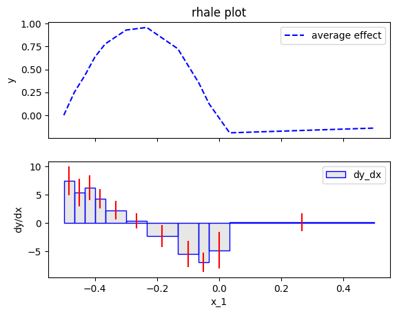
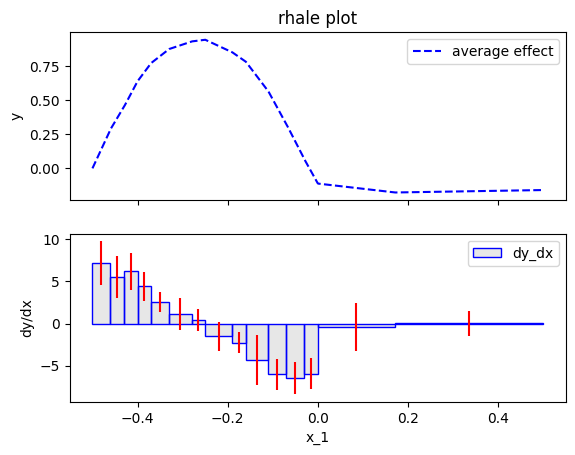
Figure 4: RHALE approximation using DynamicProgramming (left) and Greedy (right).

⬇

1from effector.binning_methods import DynamicProgramming, Greedy

2from effector import RHALE

3

4# Input

5# x = .., the dataset (np.array of shape=(N,D))

6# f = .., predictive function (python callable)

7# f_der = .., the model’s derivative (python callable)

8

9# RHALE

10rhale = RHALE(data=x, model=f, model_jac=f_der)

11binning = [

12 Greedy(init_nof_bins=100, min_points_per_bin=10),

13 DynamicProgramming(max_nof_bins=20, min_points_per_bin=10)

14]

15

16for binning_method in binning:

17 rhale.fit(feat, binning_method=binning_method)

18 rhale.plot(feature=0, heterogeneity=True, centering=True)

Listing 3: Demonstrating how to use Effector to approximate the RHALE effect for $x_{1}$ using Dynamic Programming and Greedy optimization.

C.1.3 PDP, d-PDP, ICE, d-ICE

Definition on the synthetic example:

In the synthetic example, the PDP for feature $x_{1}$ is given by:

$$f^{\mathtt{PDP}}(x_{1}) =\mathbb{E}_{x_{2},x_{3}}\left[f(x_{1},x_{2},x_{3})\right]$$ (25)

$$=\mathbb{E}_{x_{2}}\mathbb{E}_{x_{3}}\left[\sin(2\pi x_{1})(\mathbf{1}_{x_{1}<0}-2\mathbf{1}_{x_{3}<0})+x_{1}x_{2}+x_{2}\right]$$ (26)

$$=\sin(2\pi x_{1})\mathbf{1}_{x_{1}<0}+\mathbb{E}_{x_{3}}\left[-2\sin(2\pi x_{1})\mathbf{1}_{x_{3}<0}\right]+\mathbb{E}_{x_{2}}\left[x_{1}x_{2}+x_{2}\right]$$ (27)

$$=\sin(2\pi x_{1})(\mathbf{1}_{x_{1}<0}-2\mathbb{E}_{x_{3}}\left[\mathbf{1}_{x_{3}<0})\right]$$ (28)

$$=\sin(2\pi x_{1})(\mathbf{1}_{x_{1}<0}-2\frac{5}{6})$$ (29)

$$=\sin(2\pi x_{1})(\mathbf{1}_{x_{1}<0}-\frac{5}{3})$$ (30)

and the ICE plot for the $i$-th instance is given by:

$$f^{\mathtt{ICE}}_{i}(x_{1})=\sin(2\pi x_{1})(\mathbf{1}_{x_{1}<0}-2\mathbf{1}_{x_{3}^{i}<0})+x_{1}x_{2}^{i}$$ (31)

The PDP-ICE is shown in Figure 5(Left). Additionally, the d-PDP for feature $x_{1}$ is given by:

$$f^{\mathtt{d-PDP}}(x_{1}) =\mathbb{E}_{x_{2},x_{3}}\left[\frac{\partial f}{\partial x_{1}}(x_{1},x_{2},x_{3})\right]$$ (32)

$$=\mathbb{E}_{x_{2}}\mathbb{E}_{x_{3}}\left[2\pi\cos(2\pi x_{1})(\mathbf{1}_{x_{1}<0}-2\mathbf{1}_{x_{3}<0})+x_{2}\right]$$ (33)

$$=2\pi\cos(2\pi x_{1})(\mathbf{1}_{x_{1}<0}-2\frac{5}{6})$$ (34)

and the d-ICE plot for the $i$-th instance is given by:

$$f^{\mathtt{d-ICE}}_{i}(x_{1})=2\pi\cos(2\pi x_{1})(\mathbf{1}_{x_{1}<0}-2\mathbf{1}_{x_{3}^{i}<0})$$ (35)

which is shown in Figure 5(Right). We observe that the PDP-based methods treat the individual features as independent which leads to a non-zero effect for $x_{1}$ when $x_{1}>0$. Given the knowledge of the data-generating distribution, where $x_{3}\approx x_{1}$, we can say that this effect is misleading.

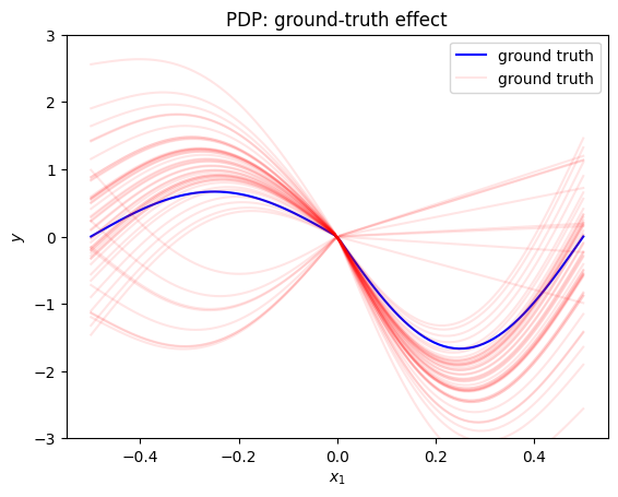
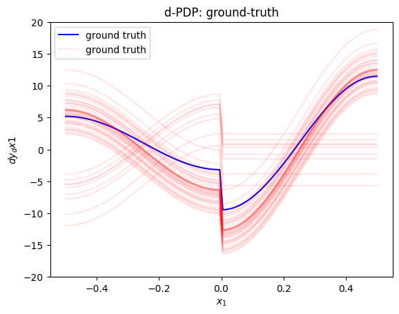
Figure 5: PDP-ICE (left) and d-PDP-ICE (right) definition on the synthetic example.

Approximation using Effector.

Listing 4 shows how to use Effector to approximate the PDP and d-PDP effect for $x_{1}$. The outputs are shown in Figure 6. We observe that the PDP-ICE (left) and d-PDP-ICE (right) approximations are very close to the respective definitions (Figure 5).

⬇

1from effector import PDP, dPDP

2

3# Input

4# x = .., the dataset (np.array of shape=(N,D))

5# f = .., predictive function (python callable)

6

7# PDP

8PDP(data=x, model=f).plot(feature=0, centering=True, heterogeneity="ice")

9

10# d-PDP

11dPDP(data=x, model=f, nof_instances=100).plot(feature=0, centering=False, heterogeneity="ice")

Listing 4: Listing showing how to use Effector to approximate the PDP and d-PDP effect for $x_{1}$.

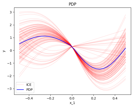
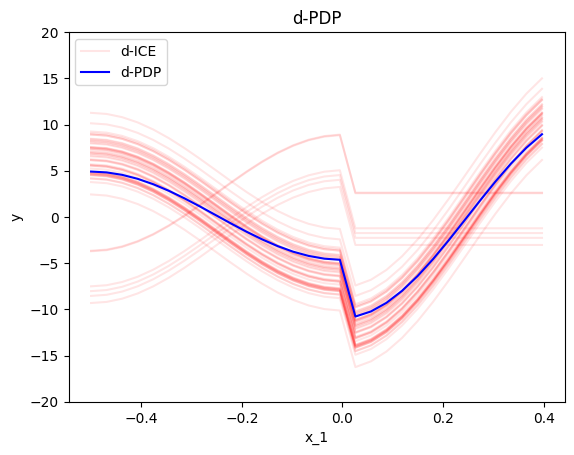
Figure 6: PDP-ICE approximation (left) and d-PDP-ICE approximation (right) on the synthetic example.

C.1.4 SHAP Dependence Plot

Definition on the synthetic example.

Finding the SHAP-DP of the $j$-th feature of the $i$-th instance requires the computation of the value of all coalitions.

$$v(\emptyset) =\mathbb{E}_{x_{1},x_{2},x_{3}}\left[\sin(2\pi x_{1})\mathbf{1}_{x_{1}<0}-2\sin(2\pi x_{1})\mathbf{1}_{x_{3}<0}+x_{1}x_{2}+x_{2}\right]$$ (36)

$$=-\frac{5}{6\pi}+0+0+0$$ (37)

$$=-\frac{5}{6\pi}$$ (38)

$$v(\{1\}) =\mathbb{E}_{x_{2},x_{3}}\left[\sin(2\pi x_{1})\mathbf{1}_{x_{1}<0}-2\sin(2\pi x_{1})\mathbf{1}_{x_{3}<0}+x_{1}x_{2}+x_{2}\right]$$ (39)

$$=\sin(2\pi x_{1})\mathbf{1}_{x_{1}<0}-\frac{5}{3}\sin(2\pi x_{1})+0+0$$ (40)

$$=\sin(2\pi x_{1})(\mathbf{1}_{x_{1}<0}-\frac{5}{3})$$ (41)

$$v(\{2\}) =\mathbb{E}_{x_{1},x_{3}}\left[\sin(2\pi x_{1})\mathbf{1}_{x_{1}<0}-2\sin(2\pi x_{1})\mathbf{1}_{x_{3}<0}+x_{1}x_{2}+x_{2}\right]$$ (42)

$$=-\frac{5}{6\pi}+0-\frac{1}{6}x_{2}+x_{2}$$ (43)

$$=-\frac{5}{6\pi}+\frac{5}{6}x_{2}$$ (44)

$$v(\{3\}) =\mathbb{E}_{x_{1},x_{2}}\left[\sin(2\pi x_{1})\mathbf{1}_{x_{1}<0}-2\sin(2\pi x_{1})\mathbf{1}_{x_{3}<0}+x_{1}x_{2}+x_{2}\right]$$ (45)

$$=-\frac{5}{6\pi}+0+0+0$$ (46)

$$=-\frac{5}{6\pi}$$ (47)

$$v(\{1,2\}) =\mathbb{E}_{x_{3}}\left[\sin(2\pi x_{1})\mathbf{1}_{x_{1}<0}-2\sin(2\pi x_{1})\mathbf{1}_{x_{3}<0}+x_{1}x_{2}+x_{2}\right]$$ (48)

$$=\sin(2\pi x_{1})\mathbf{1}_{x_{1}<0}-\frac{5}{3}\sin(2\pi x_{1})+x_{1}x_{2}+x_{2}$$ (49)

$$v(\{1,3\}) =\mathbb{E}_{x_{2}}\left[\sin(2\pi x_{1})\mathbf{1}_{x_{1}<0}-2\sin(2\pi x_{1})\mathbf{1}_{x_{3}<0}+x_{1}x_{2}+x_{2}\right]$$ (50)

$$=\sin(2\pi x_{1})\mathbf{1}_{x_{1}<0}-2\sin(2\pi x_{1})\mathbf{1}_{x_{3}<0}+0+0$$ (51)

$$=\sin(2\pi x_{1})(\mathbf{1}_{x_{1}<0}-2\mathbf{1}_{x_{3}<0})$$ (52)

$$v(\{2,3\}) =\mathbb{E}_{x_{1}}\left[\sin(2\pi x_{1})\mathbf{1}_{x_{1}<0}-2\sin(2\pi x_{1})\mathbf{1}_{x_{3}<0}+x_{1}x_{2}+x_{2}\right]$$ (53)

$$=-\frac{5}{6\pi}+0-\frac{1}{6}x_{2}+x_{2}$$ (54)

$$=-\frac{5}{6\pi}+\frac{5}{6}x_{2}$$ (55)

$$v(\{1,2,3\}) =\sin(2\pi x_{1})\mathbf{1}_{x_{1}<0}-2\sin(2\pi x_{1})\mathbf{1}_{x_{3}<0}+x_{1}x_{2}+x_{2}$$ (56)

The contribution of feature $x_{1}$ when entering in any possible coalition is:

$$\Delta_{\emptyset,1} =v(\{1\})-v(\emptyset)$$ (57)

$$=\sin(2\pi x_{1})(\mathbf{1}_{x_{1}<0}-\frac{5}{3})+\frac{5}{6\pi}$$ (58)

$$\Delta_{\{2\},1} =v(\{1,2\})-v(\{2\})$$ (59)

$$=\sin(2\pi x_{1})\mathbf{1}_{x_{1}<0}-\frac{5}{3}\sin(2\pi x_{1})+x_{1}x_{2}+\frac{1}{6}x_{2}+\frac{5}{6\pi}$$ (60)

$$\Delta_{\{3\},1} =v(\{1,3\})-v(\{3\})$$ (61)

$$=\sin(2\pi x_{1})(\mathbf{1}_{x_{1}<0}-2\mathbf{1}_{x_{3}<0})+\frac{5}{6\pi}$$ (62)

$$\Delta_{\{2,3\},1} =v(\{1,2,3\})-v(\{2,3\})$$ (63)

$$=\sin(2\pi x_{1})(\mathbf{1}_{x_{1}<0}-2\mathbf{1}_{x_{3}<0}))+x_{1}x_{2}+\frac{1}{6}x_{2}+\frac{5}{6\pi}$$ (64)

Therefore, the SHAP value of the first feature of a particular instance $i$ is:

$$\phi_{1}^{i} =\frac{1}{3}\Delta_{\{0\},1}+\frac{1}{6}\Delta_{\{2\},1}+\frac{1}{6}\Delta_{\{3\},1}+\frac{1}{3}\Delta_{\{2,3\},1}$$ (65)

$$=\sin(2\pi x_{1})\mathbf{1}_{x_{1}<0}-\sin(2\pi x_{1})\mathbf{1}_{x_{3}<0}-\frac{5}{6}\sin(2\pi x_{1})+\frac{1}{2}x_{1}x_{2}+\frac{1}{32}x_{2}+\frac{5}{6\pi}$$ (66)

$$\approx-\frac{5}{6}\sin(2\pi x_{1})+\frac{1}{2}x_{1}x_{2}+\frac{1}{32}x_{2}+\frac{5}{6\pi}$$ (67)

and the SHAP-DP, $f^{\mathtt{SHAP-DP}}(x_{1})$, is given by a one-dimensional spline fit to $\{x_{s}^{i},\hat{\phi}_{s}^{i}\}_{i=1}^{N}$ as shown in Figure 7 (left).

Approximation using Effector.

In Listing 5, we show how to use Effector to approximate the SHAP-DP for the first feature. In Figure 7, we observe that the SHAP-DP approximation is very close to the definition. As was the case with the PDP-based plots, SHAP-DP also treats the individual features as independent, leading to a non-zero effect for $x_{1}$ when $x_{1}>0$.

⬇

1from effector import SHAPDependence

2

3# Input

4# x = .., the dataset (np.array of shape=(N,D))

5# f = .., predictive function (python callable)

6

7# SHAP-DP

8SHAPDependence(data=x, model=f).plot(feature=0, centering=True, heterogeneity="shap_values")

Listing 5: Listing showing how to use Effector to approximate the SHAP-DP for $x_{1}$.

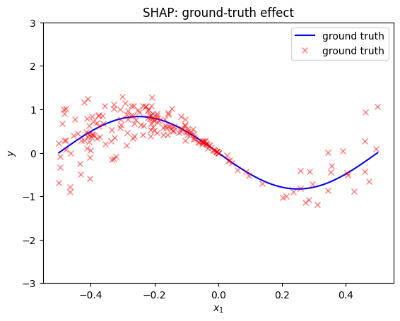
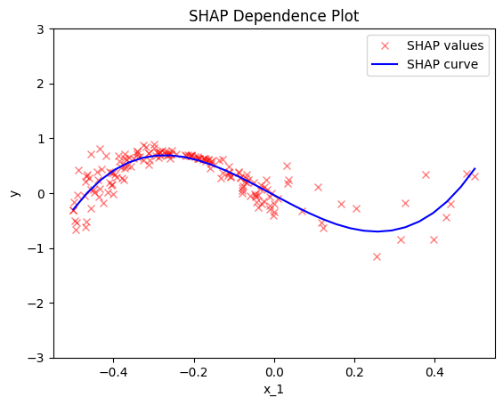
Figure 7: SHAP Dependence Plot definition (left) and approximation (right).

C.1.5 Conclusion

In this illustration, we showcase how Effector is utilized to generate global effect plots. The example highlights the simplicity of Effector’s API, typically requiring just one or two lines of code for plot generation. Additionally, the consistency of the API across various methods facilitates users in effortlessly comparing the outputs of different methods. As demonstrated, within the realm of global effect plots, there is no singular ground-truth effect. Hence, users typically seek to compare the effects obtained from different methods.

We also show that under highly-correlated features, ALE-based methodologies emerge as more reliable. In the provided example, only ALE-based techniques accurately depict that the effect of $x_{1}$ on the output diminishes to zero for $x_{1}>0$. Conversely, other methods depict a sinusoidal effect for $x_{1}>0$ due to their implicit assumption of feature independence. Additionally, we emphasize that within ALE-based frameworks, RHALE emerges as a faster and more precise approximation of the ALE definition, leveraging automatic-differentiation for speed and automatic bin-splitting for precision.

C.2 Regional Effect: Comparative study of Effector’s methods

This example shows how to use Effector for generating regional effect plots. Regional effect plots are a powerful tool for visualizing the effect of a feature on the output of a model across different regions of the feature space.

C.2.1 Problem set-up

The data generating distribution is $X_{i}\sim p(x_{i})=\mathcal{U}(x_{i};-1,1)$, for $i=\{1,2,3\}$ and the ‘black-box’ function is $f(x)=3x_{1}I_{x_{3}>0}-3x_{1}I_{x_{3}\leq 0}+x_{3}$. The terms $3x_{1}I_{x_{3}>0}$ and $3x_{1}I_{x_{3}\leq 0}$ are the ones that provoke heterogeneity in the effect of $x_{1}$. It is immediate to see that if splitting the feature space into two regions, one where $x_{3}>0$ and another where $x_{3}\leq 0$, the heterogeneity in the effect of $x_{1}$ becomes zero.

C.3 ALE and RHALE

Listing 6 shows how to use Effector to obtain regional effects using RHALE. For obtaining regional ALE effects, the only difference would be using RegionalALE instead of RegionalRHALE. At line 18, we define that an additional split is only allowed if the heterogeneity drops over 60% (0.6). At line 20, we define that the number of candidate splits for numerical features is 11. After fitting the model, we can visualize the partitioning of the feature space at line 23 using the method .show_partitioning(). The printed output informs that the feature space is split into two regions, $x_{3}\leq 0$ with 496 and $x_{3}>0$ with 504 instances, respectively. The split provokes a heterogeneity drop of 100%, from $5.94$ to $0.0$. Finally, we can visualize the global RHALE effect at line 34 and the regional effects at lines 37 and 38. The outputs are shown in Figure 8.

For features $x_{2}$ and $x_{3}$, the algorithm does not split in subspaces because the heterogeneity of the global effect is already zero. The outputs are shown in Figure 9.

⬇

1from effector import RegionalRHALE

2from effector.binning_methods import Fixed

3

4# Input

5# x = .., the dataset (np.array of shape=(N,D))

6# f = .., predictive function (python callable)

7# f_der = .., the model’s derivative (python callable)

8

9regional_rhale = effector.RegionalRHALE(

10 data=x,

11 model=f,

12 model_jac=f_der

13)

14

15binning_method = Fixed(11, min_points_per_bin=0)

16regional_rhale.fit(

17 features="all",

18 heter_pcg_drop_thres=0.6,

19 binning_method=binning_method,

20 nof_candidate_splits_for_numerical=11

21)

22

23regional_rhale.show_partitioning(features=0)

24# Feature 0 - Full partition tree:

25# Node id: 0, name: x1, heter: 5.94 || nof_instances: 1000 || weight: 1.00

26# Node id: 1, name: x1 | x3 <= -0.0, heter: 0.00 || nof_instances: 496 || weight: 0.50

27# Node id: 2, name: x1 | x3 > -0.0, heter: 0.00 || nof_instances: 504 || weight: 0.50

28# --------------------------------------------------

29# Feature 0 - Statistics per tree level:

30# Level 0, heter: 5.94

31# Level 1, heter: 0.00 || heter drop: 5.94 (100.00%)

32

33# global effect

34regional_rhale.plot(feature=0, node_idx=0, heterogeneity="std", centering=True)

35

36# regional effect

37regional_rhale.plot(feature=0, node_idx=1, heterogeneity="std", centering=True)

38regional_rhale.plot(feature=0, node_idx=2, heterogeneity="std", centering=True)

Listing 6: Listing showing how to use Effector for obtaning regional effects using RHALE.

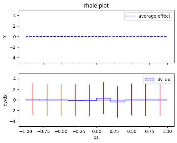
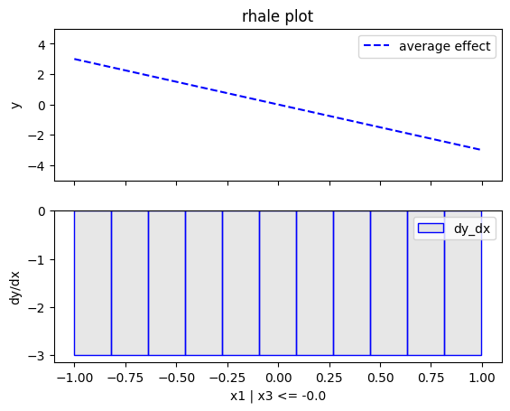
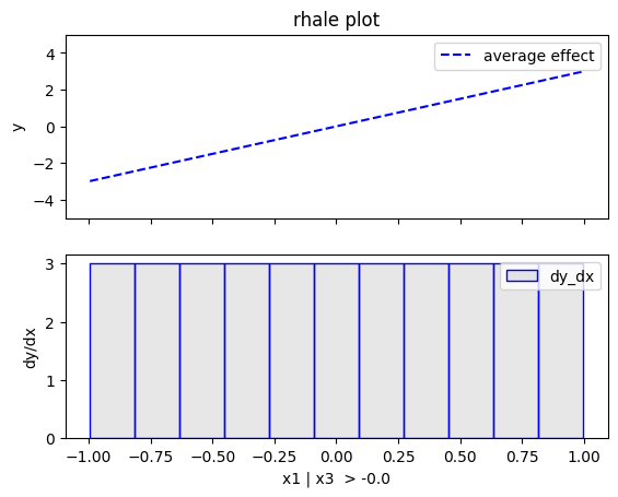
Figure 8: Top: Global RHALE effect for feature $x_{1}$. Bottom: Regional RHALE effect for feature $x_{1}$ in the regions $x_{3}\leq 0$ (left) and $x_{3}>0$ (right).

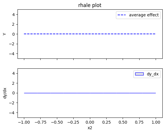
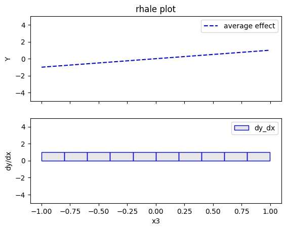
Figure 9: Global RHALE effect for feature $x_{2}$ (left) and $x_{3}$ (right).

C.4 PDP-ICE

Listing 6 shows how to use Effector to obtain regional effects using PDP-ICE. The process is identical for obtaining regional effects with d-PDP and d-ICE, with the only difference being that the method used would be RegionalDerivativePDP instead of RegionalPDP. In line 11, we define that an additional split is only allowed if the heterogeneity drops over 30% (0.3). In line 12, we define that the number of candidate splits for numerical features is 11. After fitting the model, we can visualize the partitioning of the feature space at line 15. The printed output informs that the feature space is split into two regions, $x_{3}\leq 0$ with 496 and $x_{3}>0$ with 504 instances, respectively. The split provokes a heterogeneity drop of 83.59%, from $1.74$ to $0.29$. Finally, we can visualize the global PDP effect at line 36 and the regional effects at lines 39 and 40. The outputs are shown in Figure 10.

It is interesting to notice that apart from $x_{1}$ the PDP-ICE method finds subspaces for $x_{3}$. As shown in lines 25-32 of Listing 4, the algorithm finds that by splitting in $x_{1}\leq 0$ and $x_{1}>0$, the heterogeneity of the global effect of $x_{3}$ drops from $1.76$ to $0.86$, a drop of 51.24%. The outputs are shown in Figure 11. This happens because due to PDP formula there is an offset of $\pm 6x_{1}^{i}$ at $x_{1}=0$. In the subspace $x_{1}\leq 0$, the offset is $-6x_{1}^{i}$ and in the subspace $x_{1}>0$, the offset is $6x_{1}^{i}$. For feature $x_{2}$ and $x_{3}$, the algorithm does not split in subspaces.

⬇

1from effector import RegionalPDP

2

3# Input

4# x = .., the dataset (np.array of shape=(N,D))

5# f = .., predictive function (python callable)

6# f_der = .., the model’s derivative (python callable)

7

8regional_pdp = effector.RegionalPDP(data=x, model=f)

9regional_pdp.fit(

10 features="all",

11 heter_pcg_drop_thres=0.3,

12 nof_candidate_splits_for_numerical=11

13)

14

15[regional_pdp.show_partitioning(features=i) for i in [0, 2]]

16# Feature 0 - Full partition tree:

17# Node id: 0, name: x1, heter: 1.74 || nof_instances: 1000 || weight: 1.00

18# Node id: 1, name: x1 | x3 <= -0.0, heter: 0.28 || nof_instances: 496 || weight: 0.50

19# Node id: 2, name: x1 | x3 > -0.0, heter: 0.29 || nof_instances: 504 || weight: 0.50

20# --------------------------------------------------

21# Feature 0 - Statistics per tree level:

22# Level 0, heter: 1.74

23# Level 1, heter: 0.29 || heter drop: 1.45 (83.59%)

24

25# Feature 2 - Full partition tree:

26# Node id: 0, name: x3, heter: 1.76 || nof_instances: 1000 || weight: 1.00

27# Node id: 1, name: x3 | x1 <= -0.0, heter: 0.85 || nof_instances: 507 || weight: 0.51

28# Node id: 2, name: x3 | x1 > -0.0, heter: 0.87 || nof_instances: 493 || weight: 0.49

29# --------------------------------------------------

30# Feature 2 - Statistics per tree level:

31# Level 0, heter: 1.76

32# Level 1, heter: 0.86 || heter drop: 0.90 (51.24%)

33

34for i in [0, 1]:

35 # Global effect

36 regional_pdp.plot(feature=0, node_idx=0, heterogeneity="ice", centering=True)

37

38 # regional effect

39 regional_pdp.plot(feature=0, node_idx=1, heterogeneity="ice", centering=True)

40 regional_pdp.plot(feature=0, node_idx=2, heterogeneity="ice", centering=True)

Listing 7: Listing showing how to use Effector for obtaning regional effects using PDP-ICE.

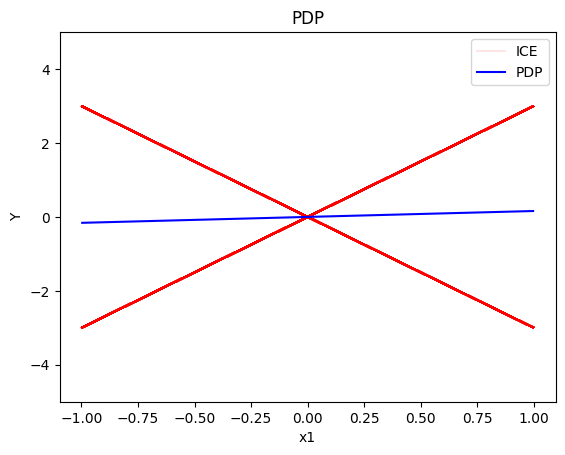
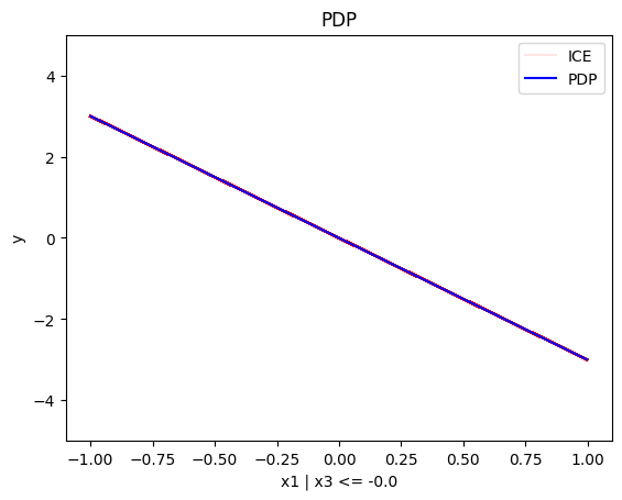
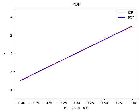
Figure 10: Left: Global PDP effect for feature $x_{1}$. Middle and Right: Regional PDP effect for feature $x_{1}$ in the regions $x_{3}\leq 0$ (left) and $x_{3}>0$

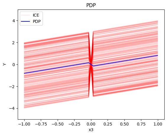
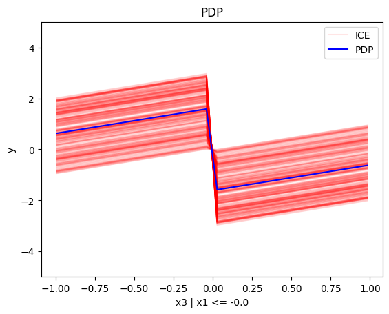
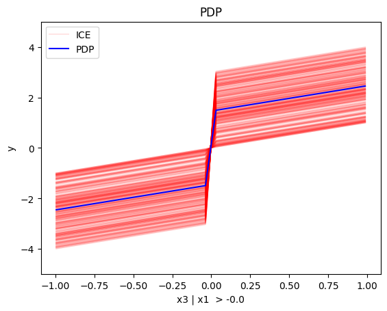
Figure 11: Left: Global PDP effect for feature $x_{3}$. Middle and Right: Regional PDP effect for feature $x_{3}$ in the regions $x_{1}\leq 0$ (left) and $x_{1}>0$.

C.5 SHAP-DP

Listing 8 shows how to use Effector to obtain regional effects using RHALE. The process is identical for obtaining regional ALE effects, with the only difference being that the method used would be RegionalALE instead of RegionalRHALE. At line 18, we define that an additional split is only allowed if the heterogeneity drops over 60% (0.6). In line 20, we define that the number of candidate splits for numerical features is 11. After fitting the model, we can visualize the partitioning of the feature space at line 22. The printed output informs that the feature space is split into two regions, $x_{3}\leq 0$ with 496 and $x_{3}>0$ with 504 instances, respectively. The split provokes a heterogeneity drop of 100%, from $5.94$ to $0.0$. Finally, we can visualize the global ALE effect at line 24 and the regional effects at lines 24 and 25. The outputs are shown in Figure 12.

For features $x_{2}$ and $x_{3}$, the algorithm does not split into subspaces. For $x_{2}$ this happens because the heterogeneity of the global effect is already zero. For $x_{3}$ there is some heterogeneity in the global effect, but there is no split that can reduce it over 60%. The outputs are shown in Figure 13.

⬇

1from effector import RegionalRHALE

2from effector.binning_methods import Fixed

3

4# Input

5# x = .., the dataset (np.array of shape=(N,D))

6# f = .., predictive function (python callable)

7

8regional_shap = effector.RegionalSHAP(data=x, model=f)

9

10regional_shap.fit(

11 features="all",

12 heter_pcg_drop_thres=0.6,

13 nof_candidate_splits_for_numerical=11

14)

15

16regional_shap.show_partitioning(features=0)

17# Feature 0 - Full partition tree:

18# Node id: 0, name: x1, heter: 0.80 || nof_instances: 100 || weight: 1.00

19# Node id: 1, name: x1 | x3 <= -0.0, heter: 0.00 || nof_instances: 49 || weight: 0.49

20# Node id: 2, name: x1 | x3 > -0.0, heter: 0.00 || nof_instances: 51 || weight: 0.51

21# --------------------------------------------------

22# Feature 0 - Statistics per tree level:

23# Level 0, heter: 0.80

24# Level 1, heter: 0.00 || heter drop: 0.80 (100.00%)

25

26# global effect

27regional_shap.plot(feature=0, node_idx=0, heterogeneity="shap_values", centering=True)

28

29# regional effect

30regional_shap.plot(feature=0, node_idx=1, heterogeneity="shap_values", centering=True)

31regional_shap.plot(feature=0, node_idx=2, heterogeneity="shap_values", centering=True)

Listing 8: Listing showing how to use Effector for obtaning regional effects using SHAP-DP.

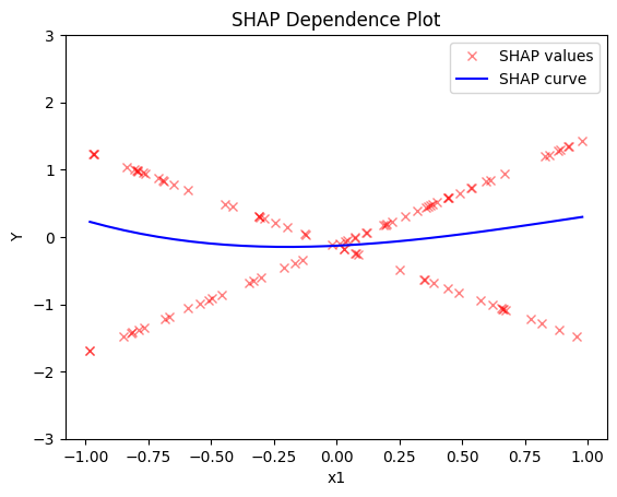
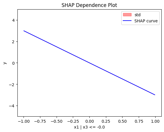
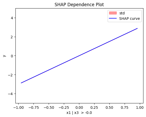
Figure 12: Left: Global SHAP-DP for feature $x_{1}$. Middle and Right: Regional SHAP-DP effect for feature $x_{1}$ in the regions $x_{3}\leq 0$ (left) and $x_{3}>0$.

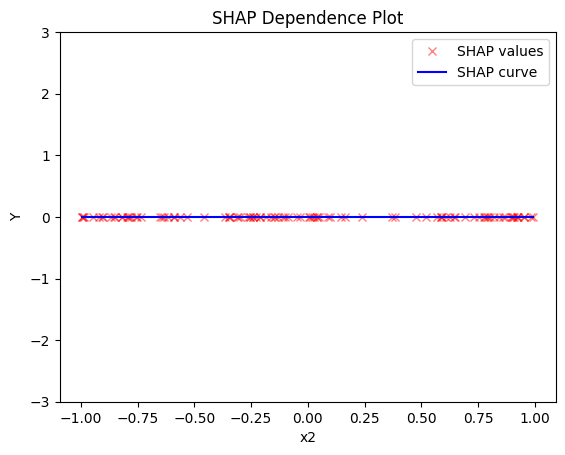
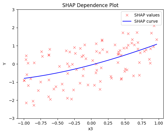
Figure 13: Global SHAP-DP for feature $x_{2}$ (left) and $x_{3}$ (right).

Appendix D Real Example

In this section, we illustrate the use of Effector on a real-world dataset.

D.1 The Bike-Sharing dataset

The Bike-Sharing Dataset contains the hourly and daily count of rental bikes between the years 2011 and 2012 in Capital bikeshare system with the corresponding weather and seasonal information.

Preprocessing and Model fitting.

The dataset contains 14 features with information about the day-type, e.g., month, hour, which day of the week, whether it is working-day, and the weather conditions, e.g., temperature, humidity, wind speed, etc. The target variable is the number of bike rentals per hour. The dataset contains 17,379 instances.

We keep 11 features; $X_{\mathtt{season}}$ (1: winter, 2: spring, 3: summer, 4: fall), $X_{\mathtt{yr}}$ (0: 2011, 1: 2012), $X_{\mathtt{mnth}}$ (1 to 12), $X_{\mathtt{hr}}$ (0 to 23), $X_{\mathtt{holiday}}$ (0: no, 1: yes), $X_{\mathtt{weekday}}$ (0 to 6), $X_{\mathtt{workingday}}$ (0: no, 1: yes), $X_{\mathtt{weathersit}}$ (1: clear, 2: mist, 3: light rain, 4: heavy rain), $X_{\mathtt{temp}}$ (normalized temperature), $X_{\mathtt{hum}}$ (normalized humidity), and $X_{\mathtt{windspeed}}$ (normalized wind speed). The target variable $Y_{\mathtt{cnt}}$ is the number of bike rentals per hour, which ranges from $1$ to $977$, with a mean of $189.5$ and a standard deviation of $181.4$.

We fit a fully connected neural network with 3 hidden layers of 1024, 512, and 256 neurons, respectively, using the TensorFlow library. We use the Mean Squared Error as the loss function and the Adam optimizer with a learning rate of $0.001$. We train the model for 20 epochs with a batch size of 512.

Global effect plots.

In Figure 15, we illustrate the PDP-ICE and Figure 14 the RHALE effect for all features. The plots reveal a high degree of concordance between the PDP and RHALE explanations across all features. Some minor differences are the following. $X_{\mathtt{year}}$ exhibits a more pronounced positive effect in RHALE compared to PDP when transitioning from 2011 to 2012. Conversely, for $X_{\mathtt{holiday}}$, the RHALE effect appears more negative than in PDP when shifting from a non-holiday to a holiday. Finally, for $X_{\mathtt{workingday}}=1$, the effect appears more positive in RHALE than in PDP.

Of particular interest is the observation that among all features, the hour of the day ($X_{\mathtt{hr}}$) exerts by far the most significant impact on bike rental numbers. The PDP and RHALE effect of $X_{\mathtt{hr}}$ shows two peaks, occurring at 8:00 and 17:00, respectively. This pattern aligns with the typical usage of bikes for commuting to and from work. Subsequently, we delve deeper into the analysis of $X_{\mathtt{hr}}$ utilizing regional effect plots.

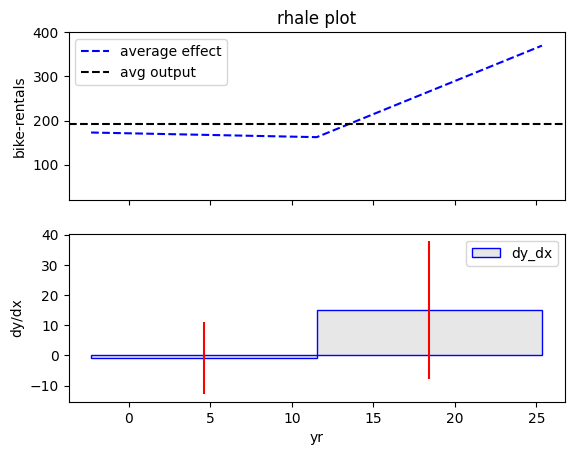
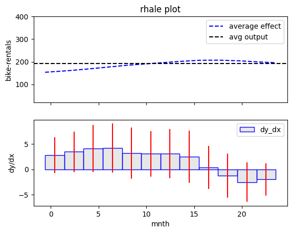
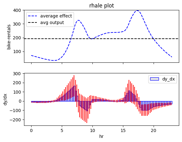
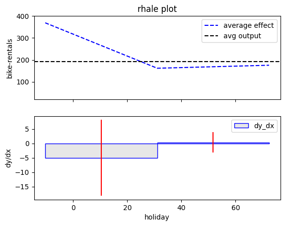
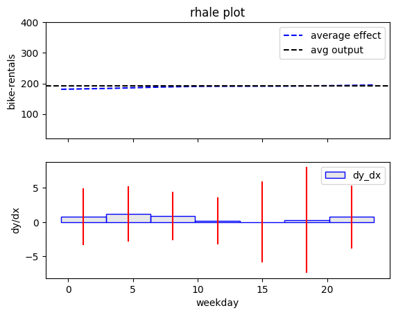
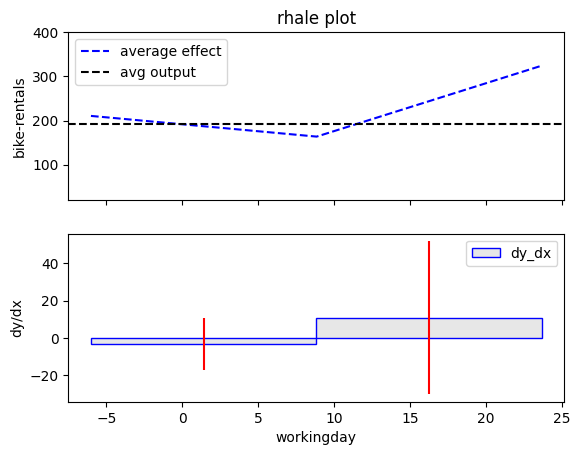
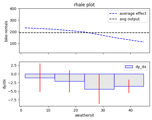
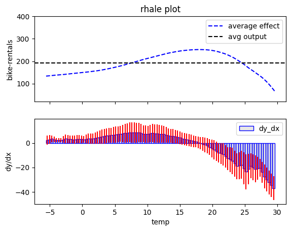
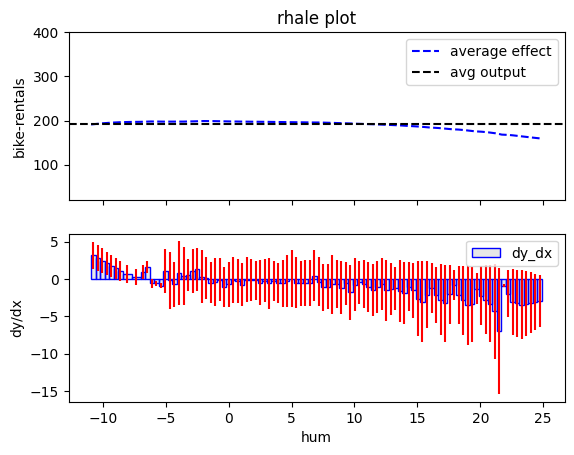
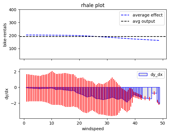
Figure 14: RHALE effect for all the features.

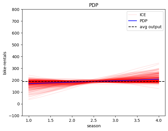
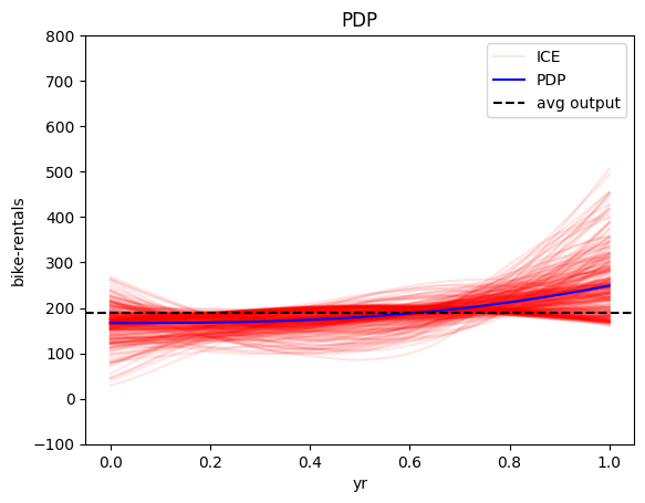
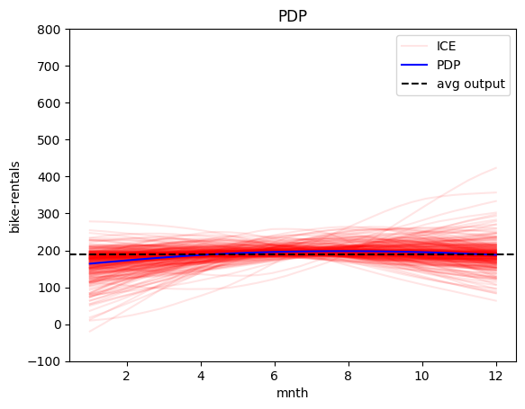
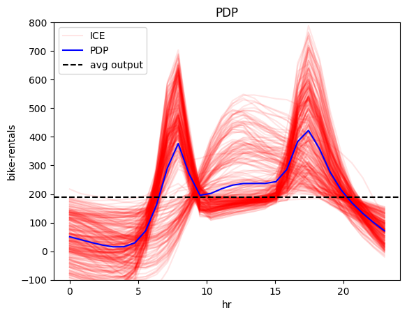
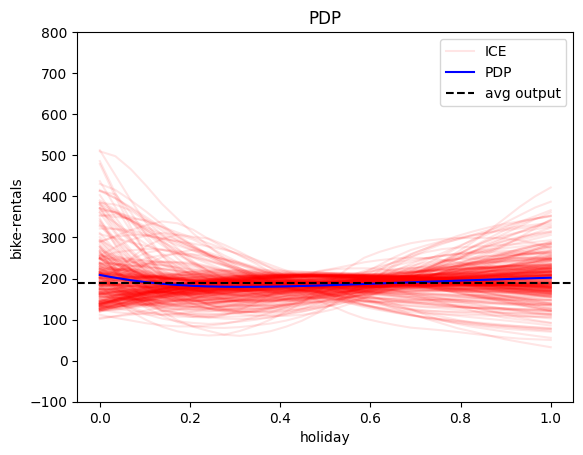
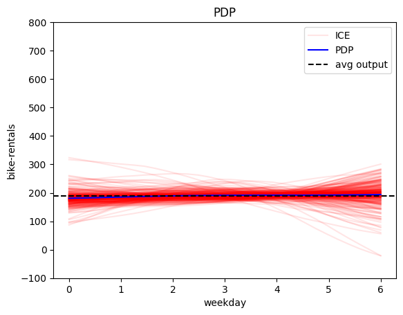
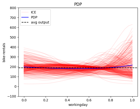
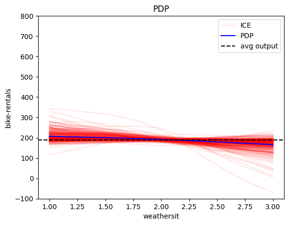
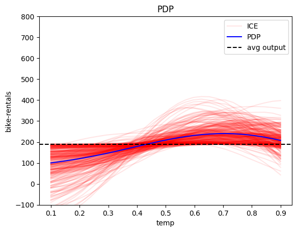
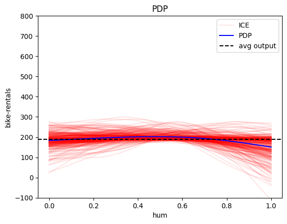
Figure 15: PDP-ICE effect for all the features.

Regional effect plots.

We further analyze the effect of the hour of the day ($X_{\mathtt{hr}}$) on bike rentals using regional effect plots. In Figure 17, we illustrate the PDP-ICE effect for $X_{\mathtt{hr}}$ on non-working days and working days. The plots reveal a significant difference in the effect of $X_{\mathtt{hr}}$ on bike rentals between non-working and working days. On non-working days, the effect of $X_{\mathtt{hr}}$ on bike rentals peaks at 14:00, while on working days, the effect peaks at 8:00 and 17:00. This pattern aligns with the typical usage of bikes for leisure on non-working days and commuting to and from work on working days.

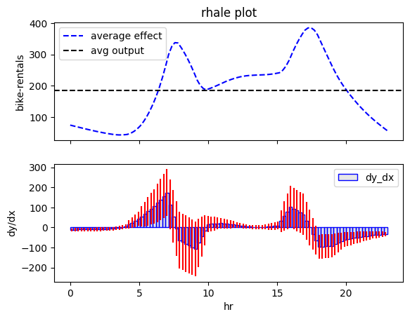
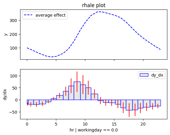
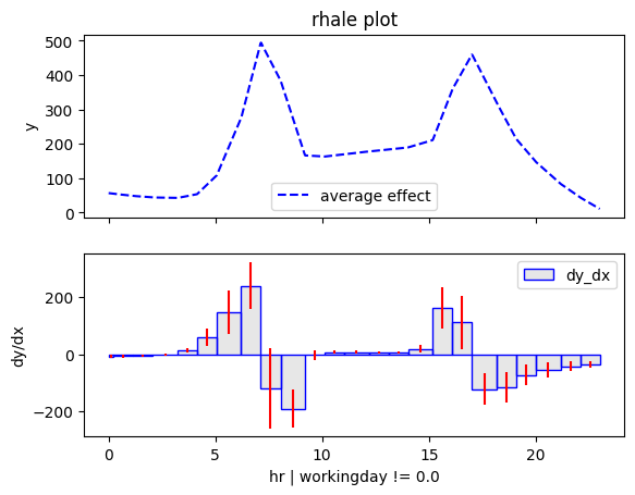
Figure 16: Top: Global RHALE effect for the temperature. Bottom: Regional RHALE effect for the temperature on non-working days (left) and working days (right).

Figure 17: Top: Global PDP effect for the temperature. Bottom: Regional PDP effect for the temperature on non-working days (left) and working days (right).

Appendix E Integration with common Machine Learning libraries

Effector is designed to be easily integrated with common machine learning libraries such as scikit-learn, TensorFlow and PyTorch. The user only needs to provide a predictive function and its derivative, if available, to use Effector with a model trained using these libraries.

In this section, we show how to use Effector with a model trained using scikit-learn (Listing 9), TensorFlow (Listing 10), and PyTorch (Listing 11). In all cases, we train a Fully Connected Neural Network (DNN) with two hidden layers of 10 neurons each. We, then, use RegionalRHALE to obtain regional effects. Note that scikit-learn does not provide auto-differentiation, so we only use the predictive function. On the other hand, TensorFlow and PyTorch provide auto-differentiation, so we use the predictive function and its derivative.

⬇

1from sklearn.neural_network import MLPRegressor

2from effector import RegionalRHALE

3

4model = MLPRegressor(

5 solver=’adam’,

6 learning_rate=’constant’,

7 hidden_layer_sizes=(10, 10),

8 learning_rate_init=0.01,

9 max_iter=100

10)

11

12model.fit(X, y)

13

14def predict(X):

15 return model.predict(X)

16

17# scikit-learn does not provide auto-differentiation.

18RegionalRHALE(data=X, model=predict).plot(feature=0, node_idx=0)

Listing 9: Integration of Effector with scikit-learn.

⬇

1import tensorflow as tf

2

3# define model

4model = tf.keras.Sequential([

5 tf.keras.layers.Dense(10, activation=’relu’),

6 tf.keras.layers.Dense(1)

7])

8

9# train model

10model.compile(optimizer=’adam’, loss=’mse’)

11model.fit(X, y, epochs=10)

12

13def predict(X: np.ndarray) -> np.ndarray:

14 return model.predict(X)

15

16def jaobian(X: np.ndarray) -> np.ndarray:

17 X = tf.convert_to_tensor(X, dtype=tf.float32)

18 with tf.GradientTape() as tape:

19 tape.watch(X)

20 y = model(X)

21 return tape.gradient(y, X).numpy()

22

23RegionalRHALE(X, predict, jacobian).plot(feature=0, node_idx=0)

Listing 10: Integration of Effector with Tensorflow.

⬇

1from torch import nn, optim

2

3class Net(nn.Module):

4 def __init__(self):

5 super(Net, self).__init__()

6 self.fc1 = nn.Linear(D, 10)

7 self.fc2 = nn.Linear(10, 1)

8

9 def forward(self, x):

10 x = self.fc1(x)

11 x = self.fc2(x)

12 return x

13

14model = Net()

15

16# train model

17optimizer = optim.Adam(model.parameters(), lr=0.01)

18criterion = nn.MSELoss()

19for epoch in range(10):

20 optimizer.zero_grad()

21 y_pred = model(X)

22 loss = criterion(y_pred, y)

23 loss.backward()

24 optimizer.step()

25

26def predict(X):

27 return model(torch.tensor(X, dtype=torch.float32)).detach().numpy()

28

29def jacobian(X):

30 X = torch.tensor(X, dtype=torch.float32)

31 X.requires_grad = True

32 y = model(X)

33 return torch.autograd.grad(y, X)[0].numpy()

34

35RegionalRHALE(X, predict, jacobian).plot(feature=0, node_idx=0)

Listing 11: Integration of Effector with PyTorch.

References

- Agarwal et al. (2021) R. Agarwal, L. Melnick, N. Frosst, X. Zhang, B. Lengerich, R. Caruana, and G. Hinton. Neural Additive Models: Interpretable Machine Learning with Neural Nets, Oct. 2021. URL http://arxiv.org/abs/2004.13912. arXiv:2004.13912 [cs, stat].
- Apley and Zhu (2020) D. W. Apley and J. Zhu. Visualizing the effects of predictor variables in black box supervised learning models. Journal of the Royal Statistical Society: Series B (Statistical Methodology), 82(4):1059–1086, 2020. Publisher: Wiley Online Library.
- Baniecki et al. (2021) H. Baniecki, W. Kretowicz, P. Piatyszek, J. Wiśniewski, and P. Biecek. dalex: Responsible Machine Learning with Interactive Explainability and Fairness in Python. Journal of Machine Learning Research, 22(214):1–7, 2021. URL http://jmlr.org/papers/v22/20-1473.html.
- Britton (2019) M. Britton. Vine: Visualizing statistical interactions in black box models. arXiv preprint arXiv:1904.00561, 2019.
- Fanaee-T and Gama (2014) H. Fanaee-T and J. Gama. Event labeling combining ensemble detectors and background knowledge. Progress in Artificial Intelligence, 2:113–127, 2014.
- (6) T. Freiesleben, G. König, C. Molnar, and A. Tejero-Cantero. Scientific Inference With Interpretable Machine Learning: Analyzing Models to Learn About Real-World Phenomena. URL http://arxiv.org/abs/2206.05487.
- Friedman (2001) J. H. Friedman. Greedy function approximation: a gradient boosting machine. Annals of statistics, pages 1189–1232, 2001.
- Friedman and Popescu (2008) J. H. Friedman and B. E. Popescu. Predictive learning via rule ensembles. The annals of applied statistics, pages 916–954, 2008. Publisher: JSTOR.
- Gkolemis et al. (2022) V. Gkolemis, T. Dalamagas, and C. Diou. Dale: Differential accumulated local effects for efficient and accurate global explanations. In Asian Conference on Machine Learning (ACML), Oct. 2022.
- Gkolemis et al. (2023a) V. Gkolemis, T. Dalamagas, E. Ntoutsi, and C. Diou. Rhale: Robust and heterogeneity-aware accumulated local effects. In ECAI 2023, pages 859–866. IOS Press, 2023a.
- Gkolemis et al. (2023b) V. Gkolemis, A. Tzerefos, T. Dalamagas, E. Ntoutsi, and C. Diou. Regionally additive models: Explainable-by-design models minimizing feature interactions. arXiv preprint arXiv:2309.12215, 2023b.
- Goldstein et al. (2014) A. Goldstein, A. Kapelner, J. Bleich, and E. Pitkin. Peeking Inside the Black Box: Visualizing Statistical Learning with Plots of Individual Conditional Expectation, Mar. 2014. URL http://arxiv.org/abs/1309.6392. arXiv:1309.6392 [stat].
- Herbinger et al. (2022) J. Herbinger, B. Bischl, and G. Casalicchio. REPID: Regional Effect Plots with implicit Interaction Detection, Feb. 2022. URL http://arxiv.org/abs/2202.07254. arXiv:2202.07254 [cs, stat].
- Herbinger et al. (2023) J. Herbinger, B. Bischl, and G. Casalicchio. Decomposing global feature effects based on feature interactions. arXiv preprint arXiv:2306.00541, 2023.
- Hu et al. (2020) L. Hu, J. Chen, V. N. Nair, and A. Sudjianto. Surrogate locally-interpretable models with supervised machine learning algorithms. arXiv preprint arXiv:2007.14528, 2020.
- Klaise et al. (2021) J. Klaise, A. V. Looveren, G. Vacanti, and A. Coca. Alibi Explain: Algorithms for Explaining Machine Learning Models. Journal of Machine Learning Research, 22(181):1–7, 2021. URL http://jmlr.org/papers/v22/21-0017.html.
- Lundberg and Lee (2017) S. M. Lundberg and S.-I. Lee. A unified approach to interpreting model predictions. Advances in neural information processing systems, 30, 2017.
- Mehrabi et al. (2021) N. Mehrabi, F. Morstatter, N. Saxena, K. Lerman, and A. Galstyan. A survey on bias and fairness in machine learning. ACM Computing Surveys (CSUR), 54(6):1–35, 2021. Publisher: ACM New York, NY, USA.
- Molnar et al. (2023) C. Molnar, G. König, B. Bischl, and G. Casalicchio. Model-agnostic feature importance and effects with dependent features: a conditional subgroup approach. Data Mining and Knowledge Discovery, pages 1–39, 2023.
- Pedregosa et al. (2011) F. Pedregosa, G. Varoquaux, A. Gramfort, V. Michel, B. Thirion, O. Grisel, M. Blondel, P. Prettenhofer, R. Weiss, V. Dubourg, J. Vanderplas, A. Passos, D. Cournapeau, M. Brucher, M. Perrot, and E. Duchesnay. Scikit-learn: Machine learning in Python. Journal of Machine Learning Research, 12:2825–2830, 2011.
- Ribeiro et al. (2016) M. T. Ribeiro, S. Singh, and C. Guestrin. ” why should i trust you?” explaining the predictions of any classifier. In Proceedings of the 22nd ACM SIGKDD international conference on knowledge discovery and data mining, pages 1135–1144, 2016.
- Scholbeck et al. (2022) C. A. Scholbeck, G. Casalicchio, C. Molnar, B. Bischl, and C. Heumann. Marginal effects for non-linear prediction functions. arXiv preprint arXiv:2201.08837, 2022.
- Sokol and Flach (2020) K. Sokol and P. Flach. Explainability fact sheets: A framework for systematic assessment of explainable approaches. In Proceedings of the 2020 conference on fairness, accountability, and transparency, pages 56–67, 2020.