Possible X-ray Cocoon Emission from GRB 050709

Abstract

The detection of the short gamma-ray burst (SGRB) 050709 by the HETE-2 satellite opened a new window into understanding the nature of SGRBs, offering clues about their emission mechanism and progenitors, with the crucial aid of optical follow-up observations. Here, we revisit the prompt emission of GRB 050709. Our analysis reveals an initial hard spike $\sim$200 ms long, followed by a subsequent soft tail emission lasting $\sim$300 ms. These components could be common among other SGRBs originating from binary neutron merger events, such as GW/GRB 170817A. Detailed temporal and spectral analyses indicate that the soft tail emission might be attributed to the cocoon formed by the relativistic jet depositing energy into the surrounding material. We find the necessary cocoon parameters at the breakout, as consistent with numerical simulation results. We compared the physical parameters of this cocoon with those of other SGRBs. The relatively higher cocoon pressure and temperature in GRB 050709 may indicate a more on-axis jet compared to GRB 170817A and GRB 150101B.

1 Introduction

The observation of the gravitational-wave event GW 170817 (Abbott et al., 2017a) marks a major historic event as it represents not only the first discovery of a gravitational-wave signal from a binary neutron star (BNS) merger, but also the detection of its electromagnetic (EM) counterparts. This discovery has opened a new window in multi-messenger astronomy. Thanks to these multi-wavelength observations, the following EM counterparts were associated with GW/GRB 170817A: (1) “short gamma-ray bursts (SGRBs)” (i.e., prompt emission) in the X-ray and ${\gamma}$-ray bands (Abbott et al., 2017b; Goldstein et al., 2017), (2) “kilonovae (macronovae)” in the ultraviolet, visible, and infrared bands (Arcavi et al., 2017; Chornock et al., 2017; Coulter et al., 2017; Díaz et al., 2017; Drout et al., 2017; Kilpatrick et al., 2017; Kasliwal et al., 2017; Nicholl et al., 2017; Pian et al., 2017; Smartt et al., 2017; Shappee et al., 2017; Soares-Santos et al., 2017; Tanaka et al., 2017; Utsumi et al., 2017; Valenti et al., 2017) and (3) “afterglows” from the radio to X-ray bands (D’Avanzo et al., 2018; Resmi et al., 2018; Mooley et al., 2018; Lamb et al., 2019; Ghirlanda et al., 2019; Troja et al., 2019a).

For the prompt emission of GRB 170817A, $\sim$1.7 s after the BNS merger time, gamma-rays photons were observed by Fermi/GBM for a duration of $\sim 2$ s (Goldstein et al., 2017) and INTEGRAL/SPI-ACS with a ${\sim}3{\sigma}$ confidence level (Savchenko et al., 2017). The observed isotropic equivalent luminosity is $\sim$10⁴⁷ erg/s which is 3–4 orders of magnitude lower than typical SGRBs (Abbott et al., 2017b), while the fluence, peak flux, peak energy $E_{\rm peak}$, and duration of GRB 170817A are all roughly consistent with the standard SGRBs (Goldstein et al., 2017). The time-resolved analysis of the prompt emissions revealed the existence of a short hard pulse with a non-thermal spectrum followed by a soft tail with a blackbody spectrum of $\sim 2$ s (Goldstein et al., 2017).

In recent years, analysis of SGRB events with similar temporal and spectral properties to those of GRB 170817A has been performed (Burns et al., 2018; von Kienlin et al., 2019). Burns et al. (2018) conducted the time-resolved analysis for the prompt emission of the nearby SGRB 150101B with $z=0.134$ using the Fermi/GBM data. They also found a short hard-spike component and a long soft-tail one, which is similar to GRB 170817A. The Fermi/GBM spectral analysis indicates that the soft-tail emission has a thermal origin. In addition, a kilonova was discovered for GRB 150101B (Troja et al., 2018). Thus, these two nearby SGRBs with kilonovae have in common a soft-tail component in their prompt emission, suggesting that the soft tail could be a ubiquitous property of SGRBs produced by BNS mergers. Note that in the early days of GRB observations, a soft tail was also detected from the April 27 burst in 1972 by the historical Apollo 16 observation (Metzger et al., 1974).

The High Energy Transient Explorer-2 (HETE-2) satellite (Ricker et al., 2003) detected the short gamma-ray burst GRB 050709 (Villasenor et al., 2005). This observation led to the very first detection of an optical counterpart to a short GRB (Covino et al., 2006). It was located in the outskirt of a host galaxy with an offset of 3.8 kpc from the center of the galaxy, at a redshift $z=0.16$, with non-detection of a supernova component (Fox et al., 2005). This opened a new window to multi-wavelength observations of SGRBs. In addition, Jin et al. (2016) reported that the late optical emission observed at $t_{\rm obs}>2.5$ days after GRB 050709 (in the observer frame) can be explained by a kilonova transient, Here, we present a reanalysis of the X-ray and $\gamma$-ray data of GRB 050709 observed by HETE-2. We found that it consists of a hard-spike followed by a soft-tail component in its prompt emission, in similarity to GRB 150101B and GRB 170817A. Thus, we focused on the temporal and spectral features of the soft-tail component, which had not been analyzed in previous studies. Our detailed spectral analysis shows that the soft-tail component likely originates from the thermal emission caused by the jet energy injection into the expanding ejecta material (i.e., cocoon emission; Pe’er et al. (2006); Nakar & Piran (2017); Lazzati et al. (2017a, b); Gottlieb et al. (2018); Nakar et al. (2018); Ioka & Nakamura (2018); Lazzati et al. (2018); Piro & Kollmeier (2018); Hamidani et al. (2020, 2021, 2024)). Furthermore, we estimated the physical parameters of the cocoon of GRB 050709, and compared them with those of GRB 150101B and GRB 170817A.

This paper is organized as follows: the observation of the HETE-2 and the detection of the soft-tail component are described in Section 2, the physical parameters of the cocoon emission is quantified in Section 3, the origin of the extended emission is discussed in Section 4, and our conclusion is presented in Section 5. In this paper, errors are defined as within 90% confidence level.

2 Observed Properties of GRB 050709

2.1 Overview of the observations

GRB 050709 was detected by the Wide-Field X-Ray Monitor (WXM, 2–25 keV; Shirasaki et al. (2003)) and the French Gamma Telescope (FREGATE, 6–400 keV; Atteia et al. (2003)) on board of the HETE-2 on July 9 2005, at 22:36:37 UT (denoted as $t_{\rm 0}$) (Villasenor et al., 2005). The WXM location was found by ground analysis to be right ascension (RA) +23 h 01 min 44 s and declination (dec.) $-38\mathrm{°}⁤59\mathrm{\prime }⁤52\mathrm{″}$ (J2000) with an error radius of $14.5\mathrm{\prime }$. The X-ray afterglow was observed by Chandra at $t_{\rm 0}+{\sim}2.5,16.0,16.1$ days and Swift at $t_{\rm 0}+{\sim}1.6,2.4,3.2,4.3$ days. The Swope-40 and Subaru telescope performed the optical observations in the $i^{\prime}$ and $K^{\prime}$ bands, respectively, ${\sim}1.5$ days after the trigger (Fox et al., 2005). Notably, the Gemini Multi-Object Spectrograph on the Gemini North telescope identified the redshift of the host galaxy to be $z=0.16$ (Fox et al., 2005). The Hubble Space Telescope (HST) carried out four observations in the F814W band during the initial one month after the burst (Fox et al., 2005) and found a fading optical emission likely originating from a kilonova (Jin et al., 2016). One year after the burst, the HST did not detect significant emission related to this GRB in the F814W band at the same position (Jin et al., 2016). The Very Large Telescope (VLT) also detected an optical afterglow in the $V$, $R$ and $I$ bands from July 12 to 30, 2005 (Covino et al., 2006).

2.2 Prompt emission phase

2.2.1 Lightcurves

In Fig. 1, we show the light curves of the prompt emission phase observed with WXM (2–25 keV) and FREGATE (6–400 keV). The durations of the prompt emission in the 2–25 and 30–-400 keV energy bands are $T_{\rm 90}$ = 220$\pm$50 ms and 70$\pm$10 ms, respectively (Villasenor et al., 2005), where $T_{90}$ is measured as the duration of the time interval during which 90% of the total observed counts have been detected. Our reanalysis clearly shows for the first time that the lightcurve in the initial 0.5-s interval consists of two components in the prompt emission phase as seen in GRB 170817A and GRB 150101B: (1) “Hard Spike (HS)”, which was observed at $t_{\rm 0}+0.0-0.2$ s in all energy bands (2–400 keV); and (2) “Soft Tail (ST)”, which was observed only in the soft X-ray energy range of 2–10 keV at $t_{\rm 0}+0.2-0.5$ s.

2.2.2 Significance of the soft tail emission

The detection significance of the soft-tail emission is briefly calculated to be ${\sim}5.6{\sigma}$ using the light curve in the 2–10 keV band considering the X-ray photon statistics of the GRB emission and the background fluctuation. In addition, by using the HETE-2 science tools for transient localization, we calculated the incident X and Y angles of X-rays from the hard-spike emission with respect to the WXM boresight and found it as ${\theta_{\rm x}^{\rm HS}}=-14.27^{+0.08}_{-0.03}$ deg and ${\theta_{\rm y}^{\rm HS}}=-2.12^{+0.03}_{-0.06}$ deg, respectively. The incident X and Y angles of X-rays from the soft tail emission were also calculated and found as $\theta_{\rm x}^{\rm ST}=-14.48^{+24.42}_{-0.14}$ deg and ${\theta_{\rm y}^{\rm ST}}=-2.13^{+33.60}_{-28.58}$ deg, respectively, for the soft tail. The obtained incident angles are consistent between the hard-spike and soft-tail emissions. Note that the uncertainty of the incident Y angle of the soft-tail emission is very large due to limitations of the X-ray photon statistics. Therefore, we concluded that the soft-tail emission is most likely a genuine source signal of this GRB, rather than a statistical fluctuation.

2.2.3 Spectra

For the spectral analysis, we used XSPEC version 12.12.0 (Arnaud, 1996) with the WXM and FREGATE data, and adopted the “PGstat” statistic, suitable for low photons counts (Arnaud et al., 2011). We adopted four types of spectral models, i.e., power-law (PL), cutoff PL (CPL), blackbody (BB), and multi-temperature blackbody (DISKPBB). Hence, the DISKPBB model was originally used for reproducing emission from an accretion disk with multiple-temperature blackbody components. This emission is described by $kT_{\rm disk}(r)\propto r^{-p}$, where $k$ is the Boltzmann constant, $T_{\rm disk}(r)$ represents the local disk temperature, $r$ is the distance from a compact object, and $p$ is the power-law index. The temperature at the inner disk radius is denoted by $kT_{\rm in}$. In this study, we used the DISKPBB model implemented in XSPEC to represent a modified blackbody spectrum broadened by the relativistic motion of the ejecta originating from the cocoon empirically. Similar approaches were employed in previous studies (Ryde et al., 2010; Arimoto et al., 2016).

Using these functions, our fitting results are shown in Table 2.2.3. The hard spike (HS) and the soft tail (ST) are best fit by a cutoff power-law with $E_{\mathrm{peak}}^{\mathrm{HS}}=200^{+437}_{-81}$ keV and a multi-temperature blackbody with $kT_{\rm in}=48.5^{+15.2}_{-18.5}$ keV, respectively. According to this best fit, the isotropic energy of the hard spike is $E_{\mathrm{iso}}^{\mathrm{HS}}=4.41^{+0.60}_{-0.32}\times 10^{49}\,\mathrm{erg}$, and the isotropic luminosity of the hard spike is $L_{\mathrm{iso}}^{\mathrm{HS}}=2.56^{+0.35}_{-0.19}{\times}10^{50}\,\mathrm{erg\,s^{-1}}$. In addition, for the soft tail emission spectrum shown in Fig. 2, the PGStat values of the CPL and DISKPBB models have similar values, i.e., PGstat = 93.8 (dof = 97) for CPL and PGstat = 92.7 (dof = 97) for DISKPBB. The difference of the PGstat values ($\Delta$PGstat $\sim$ 1) is not so statistically significant. Thus, the CPL is almost equivalent to the DISKPBB model, and the effective temperature of the CPL can be found to be $kT_{\rm eff}=E_{\rm peak}/2.8\sim 42$ keV using Wien’s law, which is consistent with the temperature obtained from the DISKPBB model ($kT_{\rm in}=48.5^{+15.2}_{-18.5}$ keV).

Figure 1: Composite light curve of GRB 050709 from $t_{\rm 0}$ $-1$ s to $+1$ s in different energy ranges with 10 ms/bin (blue line) and 50 ms/bin (black line), showing the short hard spike and the soft tail. The vertical lines represent the time intervals of the hard spike and the soft tail. The red line represents the background, which is the average of the count rate from $t_{\rm 0}$ - 1 s to -0.5 s. We show that the soft tail is clearly detected with a significance of $\sim 5.6\sigma$ using a binning of 50 ms for the light curve of 2–10 keV (WXM).

Figure 2: Spectral fitting and the respective residuals from $t_{\rm 0}$ +0.2 s to +0.5 s (soft tail) of GRB 050709 observed with WXM (black) and FREGATE (red). The left and right spectra are fitted by cutoff power-law function (CPL) and disk blackbody (DISKPBB), respectively.

Results of Spectral Fitting of the Prompt Emission of GRB 050709. Interval from $t_{\rm 0}$ Energy band Model $E_{\mathrm{peak}}$ Photon index, $p$ $kT_{\rm in}$ PGstat/dof Energy flux $L_{\mathrm{iso}}$ $E_{\mathrm{iso}}$ (s) (keV) (keV) (keV) ($10^{-7}$ $\mathrm{e}\mathrm{r}\mathrm{g}\,\mathrm{c}\mathrm{m}^{-2}\,\mathrm{s}^{-1}$) ($10^{49}$ $\mathrm{e}\mathrm{r}\mathrm{g}\,\mathrm{s}^{-1}$) ($10^{49}$ erg) 0–0.2 2–400 CPL $200^{+437}_{-81}$ $1.23^{+0.14}_{-0.15}$ 174.0/142 $39.5^{+5.4}_{-2.9}$ $25.6^{+3.5}_{-1.9}$ $4.41^{+0.60}_{-0.32}$ (Hard Spike) 2–400 DISKPBB $0.59^{+0.01}_{-0.02}$ $141.7^{+8.3}_{-63.3}$ 177.4/142 0.2–0.5 2–400 CPL $117^{+56}_{-55}$ $1.20^{+0.36}_{-0.52}$ 93.8/97 $9.12^{+2.04}_{-2.14}$ $5.90^{+1.32}_{-1.38}$ $1.02^{+0.23}_{-0.24}$ (Soft Tail) 2–400 BB $16.5^{+3.4}_{-2.8}$ 110.5/98 2–400 DISKPBB $0.63^{+0.10}_{-0.05}$ $48.5^{+15.2}_{-18.5}$ 92.7/97 $8.79^{+2.11}_{-1.93}$ $5.69^{+1.37}_{-1.25}$ $0.98^{+0.23}_{-0.22}$ 8–400 CPL $76.2^{+56.5}_{-17.8}$ $0.01^{+0.96}_{-1.32}$ 76.0/85 8–400 BB $16.9^{+3.5}_{-2.8}$ 79.4/86 8–400 DISKPBB $0.90^{+0.46}_{-0.46}$ $29.9^{+6.0}_{-6.0}$ 76.2/85

2.3 Extended Emission

Some SGRBs are followed by a longer, lasting ${\sim}100$ s , but a softer X-ray emission (Norris et al., 2006). The extended emission is present in GRB 050709 in the 2–10 keV band shown in Fig. 3. According to Villasenor et al. (2005), its duration is $T_{90}=130\pm 7$ s in the 2–25 keV band. As it can be seen in Fig. 3, the count rate of the background is low and fluctuating; thus the light curves were drawn for each channel and the background was subtracted by fitting with a linear function as performed in the Fermi/GBM analysis (Biltzinger et al., 2020). We performed the time-resolved spectral analysis in the early ($t_{\rm 0}$ +20–100 s) and late phases ($t_{\rm 0}$ + 100–180 s) using the same spectral models of the prompt emission. Table 2.3 shows the results of the spectral analysis of the extended emission and we find that it is hard to provide useful constraints on the spectral model due to poor photon statistics. Thus, we focus on the spectral property of the PL, characterized by a time-independent photon index of $\sim$2.4. The obtained fitting results may indicate that there is no spectral softening for this burst, although the two time intervals of the extended emission was arbitrarily defined and the uncertainties of the fitted parameters were too large to discuss their significance. Here, the extended emission of many SGRBs detected by Swift shows a significant spectral softening in previous studies (e.g., Kagawa et al. (2015, 2019)). Accordingly, for the extended emission of this GRB, we find the isotropic energy as $E_{\mathrm{iso}}=3.36^{+0.17}_{-0.43}{\times}10^{50}$ erg and the isotropic luminosity as $L_{\mathrm{iso}}=2.44^{+0.13}_{-0.31}{\times}10^{49}$ $\mathrm{e}\mathrm{r}\mathrm{g}\,\mathrm{s}^{-1}$.

Figure 3: The composite light curve of GRB 050709 from $t_{\rm 0}$ -100 s to $+250$ s in the 2–400 keV band with 1-s bin (blue line). The red line represents the background model calculated by the fitting using a linear function. We see the soft X-ray emission at $t_{\rm 0}+20$–$180$ s in the energy range of 2–10 keV (WXM). The vertical dashed lines represent the time intervals referred to in Table 2.3.

Spectral Fitting Results of Extended Emission Interval from $t_{\rm 0}$ Model $E_{\mathrm{peak}}$ Photon index, $p$ $kT$ PGstat/dof (s) (keV) (keV) 20–180 CPL $3.33^{+1.40}_{-1.12}$ $1.61^{+0.36}_{-0.86}$ 39.5/49 (Whole) PL $2.43^{+0.14}_{-0.13}$ 41.4/50 BB $1.22^{+0.11}_{-0.10}$ 44.1/50 DISKPBB $0.468^{+0.031}_{-0.031}$ $19.9^{+6.0}_{-13.8}$ 40.9/49 20–100 CPL $4.94^{+1.62}_{-1.23}$ $1.67^{+0.32}_{-0.31}$ 37.4/49 (Early phase) PL $2.35^{+0.22}_{-0.21}$ 41.1/50 BB $1.36^{+0.19}_{-0.16}$ 48.4/50 DISKPBB $0.481^{+0.031}_{-0.063}$ $33.7^{+4.8}_{-29.6}$ 41.4/49 100–180 CPL $2.71^{+2.11}_{-1.20}$ $1.67^{+0.26}_{-0.89}$ 40.9/49 (Late phase) PL $2.44^{+0.23}_{-0.21}$ 41.3/50 BB $1.16^{+0.17}_{-0.14}$ 45.2/50 DISKPBB $0.465^{+0.047}_{-0.064}$ $10.0^{+2.4}_{-6.1}$ 41.5/49

2.4 Minimum Variability Timescale

The minimum variability timescale is the time of significant flux variability of emission, which has been considered to give an upper limit on the size of the emitting region and a hint on the nature of the progenitor of the bursts (Schmidt, 1978). A temporal analysis that determines the power of the differentiated time series of the light curve can be used to estimate the observed variability timescale, $\Delta t$, by subtracting the photon counts in one time bin from the adjacent bin (Nemiroff et al., 1997). The obtained power spectrum is shown in Fig. 4 for GRB 050709 using the FREGATE light curve in the energy range of 8–400 keV during the time interval of the short bright emission ($t_{\rm 0}$ + 0.0–0.5 s). The Poisson noise due to X-ray photon statistics, which can be represented as the power-law function of $\Delta t^{-1}$ in the power spectrum, should be taken into account when estimating the variability timescale from a GRB emission. Thus, we calculated the variability timescale from the emission of this GRB that exceeds the Poisson-noise component with a confidence level greater than 3$\sigma$. For GRB 050709, the minimum variability timescale of the short bright emission at $t_{\rm 0}$ + 0.0–0.5 s in the energy range of 8–400 keV is estimated as 5.7$\pm$0.2 ms.

Figure 4: Power spectrum of the root-mean-square (RMS) amplitude of the FREGATE light curve as a function of the variability timescale $\Delta t$ for GRB 050709 at $t_{\rm 0}$ + 0.0–0.5 s in the energy range of 6–400 keV. The Poisson noise is represented as $\Delta t^{-1}$ in the power spectrum (red line). The minimum variability timescale ${\tau}_{\mathrm{min}}$ can be derived from the emission of this GRB that exceeds the Poisson-noise component at a confidence level exceeding 3$\sigma$.

For GRB 170817A observed by Fermi/GBM, the minimum variability timescale in the 10–1000 keV energy range was calculated as ${\tau}_{\mathrm{min}}$ = $0.18{\pm}0.12$ s with our method, which is consistent with ${\tau}_{\mathrm{min}}$ = 0.13$\pm$0.06 s estimated by the previous work (Goldstein et al., 2017) using the structure function estimator (Golkhou & Butler, 2014). Fig. 5 shows the observed minimum variability timescale ${\tau}_{\mathrm{min}}$ versus the GRB duration $T_{90}$ of GRB 050709, GRB 170817A, and other GRBs. This result shows that GRB 050709 belongs to the group of SGRBs with the shortest variability timescale and the shortest duration. Note that the minimum variability timescales of the hard spike and the soft tail are estimated as ${\tau}^{\mathrm{HS}}_{\mathrm{min}}$ = 2.9$\pm$0.2 ms and ${\tau}^{\mathrm{ST}}_{\mathrm{min}}$ = 50$\pm$5 ms, respectively. In the next section, the estimated minimum variability timescale of the soft tail is used to constrain the emission radius.

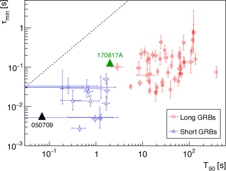
Figure 5: The minimum variability timescale vs. the GRB duration $T_{90}$, for a sample of long and short GRBs. GRB 050709 and GRB 170817A are represented as black and green triangles, respectively. The red circle and blue triangle represent long and short GRBs, respectively, taken from MacLachlan et al. (2013). The minimum variability timescale is calculated using a time interval during the prompt emission (e.g., HS+ST). The dashed black line denotes where values are equal. Note that $T_{90}$ = 70$\pm$10 ms in the 30–400 keV energy band was adopted for GRB 050709.

3 Origin of the soft tail

Previous studies showed that the electromagnetic emissions of the prompt emission and the afterglow of GRB 170817A can be explained by a structured/off-axis relativistic jet (Lazzati et al., 2017a; Troja et al., 2017; Margutti et al., 2017; Alexander et al., 2018; Haggard et al., 2017; Gill & Granot, 2018; Dobie et al., 2018; Granot et al., 2018; D’Avanzo et al., 2018; Lazzati et al., 2018; Lyman et al., 2018; Margutti et al., 2018; Mooley et al., 2018; Troja et al., 2018a; Lamb et al., 2019a; Wu & MacFadyen, 2019; Fong et al., 2019; Hajela et al., 2019; Ryan et al., 2020; Troja et al., 2020; Takahashi & Ioka, 2021; Troja et al., 2022; Hajela et al., 2022), and a jet and cocoon model (Kasliwal et al., 2017; Nakar & Piran, 2017; Gottlieb et al., 2018; Kimura et al., 2019; Hamidani & Ioka, 2023a, b). In particular, observations show that at the prompt emission phase, there is the soft tail emission with a weak thermal component in GRB 170817A(Goldstein et al., 2017). The emission mechanism of this soft tail from GRB 170817A could arise from the photosphere of the jet or the photosphere of the cocoon (Kasliwal et al., 2017; Lazzati et al., 2017b; Gottlieb et al., 2018; Ioka et al., 2019; Hamidani & Ioka, 2023b).

3.1 Cocoon model

In the following, we explore the origin of the the soft-tail emission from GRB 050709, and show that it can be explained by cocoon. First, we assume that the spectrum of the soft tail was observed as a DISKPBB model with $kT_{\mathrm{in}}\sim 49$ keV in Table 2.2.3. The isotropic luminosity of the soft tail is $L_{\rm iso}^{\rm ST}\sim 6{\times}10^{49}$ $\mathrm{e}\mathrm{r}\mathrm{g}\,\mathrm{s}^{-1}$; using $L=4{\pi}{D_{L}}^{2}F$, where $D_{L}$ is the luminosity distance and $F$ is the energy flux. $R_{\rm c}$ is the lateral width of the cocoon, immediately after the breakout. The emitting surface is $\sim\pi R_{\rm c}^{2}$, and considering the conical shape of the cocoon, one can roughly find that $R_{\rm c}$ is comparable to the cocoon’s photospheric radius (Hamidani & Ioka, 2023b) Thus, the cocoon radius $R_{\rm c}$ at the breakout time can be calculated by the following equation:

$$R_{\rm c}=\left[\frac{{\Gamma}_{\rm c}^{2}L_{\rm iso,c}}{4{\pi}{\sigma}\{T_{\rm obs,c}(1+z)\}^{4}}\left(\frac{\Omega_{\rm EM}}{\Omega}\right)\right]^{\frac{1}{2}}=\left[\frac{{\Gamma}_{\rm c}^{2}L_{\rm iso,c}}{4{\pi}{\sigma}\{T_{\rm obs,c}(1+z)\}^{4}}\left(\frac{\theta_{\rm EM}}{\theta_{\rm c}}\right)^{2}\right]^{\frac{1}{2}},$$ (1)

where ${\Gamma}_{\rm c}$ is the Lorentz factor of the cocoon, $L_{\rm iso,c}$ is the isotropic equivalent luminosity of the cocoon, $T_{\rm obs,c}$ is the observed cocoon temperature, $\sigma$ is the Stefan–Boltzmann constant, $\Omega_{\rm EM}$ is the solid angle of the electromagnetic emission, $\Omega$ is the solid angle corresponding to the physical size of the cocoon with as $\theta_{\rm c}$ its opening angle, and $\theta_{\rm EM}$ is the opening angle of the electromagnetic emission. In addition, the opening angle of the emission is $\theta_{\rm EM}\sim{\Gamma}_{\rm c}^{-1}$. Thus, Equation 1 becomes

$$R_{\rm c}=\left[\frac{L_{\rm iso,c}}{4{\pi}{\sigma}\left\{T_{\rm obs,c}(1+z)\right\}^{4}}\left(\frac{1}{\theta_{\rm c}}\right)^{2}\right]^{\frac{1}{2}}\sim 2{\times}10^{9}\,\mathrm{cm}\left(\frac{{\theta}_{\rm c}}{25^{\circ}}\right)^{-1}\left(\frac{kT_{\rm obs,c}}{49\,\mathrm{keV}}\right)^{-2}\left(\frac{L_{\rm iso,c}}{6\times 10^{49}\,\mathrm{erg\,s^{-1}}}\right)^{\frac{1}{2}}$$ (2)

According to Hamidani & Ioka (2023a), the typical value for the opening angle of the cocoon is ${\theta}_{\rm c}\sim 25^{\circ}$. The maximum cocoon radius $R_{\rm c,max}$ obtained from temporal variability $\tau_{\rm min}^{\rm ST}$ is as follows (Piran, 2005):

$$R_{\rm c,max}=4c\frac{\tau_{\rm min}^{\rm ST}}{1+z}{\Gamma}_{\rm c}^{2}\sim 2\times 10^{10}\,\mathrm{cm}\left(\frac{\tau_{\rm min}^{\rm ST}}{50\,\mathrm{ms}}\right)\left(\frac{{\Gamma}_{\rm c}}{2}\right)^{2}\left(1+z\right)^{-1},$$ (3)

where $c$ is the speed of light. The typical value for the Lorentz factor of the cocoon ${\Gamma}_{\rm c}$ at the breakout time is a few (see Hamidani & Ioka (2023a, b)), and we adopt ${\Gamma}_{\rm c}\sim 2$ in this equation. The values of $R_{\rm c}$ and $R_{\rm c,max}$ derived from Equations 2 and 3 confirm $R_{\rm c}<R_{\rm c,max}$. Assuming a radiation dominant pressure, the pressure of the cocoon can be calculated by the following equation (assuming an adiabatic index of 4/3):

$$P_{\rm c}=\frac{1}{4{{\Gamma}_{\rm c}}^{2}-1}\frac{E_{\rm th}}{V_{\rm c}}{\sim}\frac{1}{4{{\Gamma}_{\rm c}}^{2}}\frac{E_{\rm th}}{V_{\rm c}},$$ (4)

where $E_{\rm th}$ is the thermal energy of the cocoon and $V_{c}$ is its volume (for simplicity ${\Gamma}_{\rm c}\gg 1$ here). Here, the energy density is $E_{\rm th}/V_{\rm c}=4{\sigma}T_{\rm c}^{4}\Gamma_{\rm c}^{2}/c$ and $T_{\rm c}={\Gamma_{\rm c}}^{-1}T_{\rm obs,c}$ is the comoving cocoon temperature, giving

$$P_{\rm c}=\frac{\sigma}{c}\left[\frac{T_{\rm obs,c}(1+z)}{\Gamma_{\rm c}}\right]^{4}\sim 2{\times}10^{19}\,\mathrm{erg\,cm^{-3}}\left(\frac{\Gamma_{\rm c}}{2}\right)^{-4}\left(\frac{kT_{\rm obs,c}}{49\,\mathrm{keV}}\right)^{4}$$ (5)

It is worth noting that the above value of the cocoon pressure is quite consistent with the cocoon pressure as in 2D relativistic hydrodynamical simulation of jet propagation in the expanding ejecta of BNS mergers, as found in Hamidani et al. (2021). Hamidani et al. (2021) simulated the narrow jet case with the initial opening angle of the jet $\theta_{0}=6.8^{\circ}$ and $E_{\rm th}\sim 4\times 10^{46}\mathrm{erg}$, and the wide jet case with $\theta_{0}=18.0^{\circ}$ and $E_{\rm th}\sim 1\times 10^{48}\mathrm{erg}$ (see their table 1 and their definition of $\theta_{0}$), showing $\sim$0.2 s after the jet launch the cocoon pressures $P_{\rm c}\sim$ 2$\times$10¹⁹ erg cm^-3 and 1$\times$10²⁰ erg cm^-3 and the cocoon radii $R_{\rm c}\sim$ 4$\times$10⁹ cm and 2$\times$10⁹ cm for the narrow- and wide-jet cases, respectively. While the estimated cocoon radius of GRB 050709 and the simulated cocoon radii for the narrow- and wide-jet cases are within the same order of magnitude, the estimated cocoon pressure of GRB 050709 is consistent with the narrow-jet case, hence the narrow-jet scenario might be favored for this GRB in several aspects.

3.2 Comparison with other GRBs

Table 3.2 shows a comparison between three SGRBs (all having a soft tail component and evidence of kilonova emission in common): GRBs 170817A, 150101B, and 050709. Here, the spectral models for GRBs 170817, 150101B, and 050709 are represented by BB (Goldstein et al., 2017), BB (Burns et al., 2018), and DISKPBB (this work), respectively. In addition to the observed properties, the temperature and the pressure of these SGRBs are shown, including newly found results here for GRB 050709. Comparison shows that GRB 050709 has a relatively higher temperature and a much higher pressure compared to the other two SGRBs. The high temperature and pressure of the cocoon for GRB 050709 can be caused by contribution from the shocked jet part of the relativistic cocoon, rather than the shocked ejecta part of the non-relativistic cocoon. This suggests that GRB 050709 was observed with a line-of-sight closer to the jet axis, compared to the other SGRBs, while for GRB 170817A the viewing angle was estimated as $\sim 20^{\circ}$–$30^{\circ}$ (Troja et al. (2018a), Mooley et al. (2018), Abbott et al. (2017a)).

Another reason for the high temperature of the cocoon in GRB 050709 may be due to the different energy coverage between HETE-2 (2–400 keV) and Fermi-GBM (8 keV – 40 MeV; Meegan et al. (2009)). The observed spectra of the soft-tail emission for GRBs 150101B and 170817A were well fitted by BB (Goldstein et al., 2017; Burns et al., 2018). It should be noted that the lower detectable energy threshold of the Fermi-GBM ($\sim$8 keV) is close to the observed BB temperatures ($\sim$6 keV for GRB 150101B and $\sim$10 keV for GRB 1708017A; Burns et al. (2018); Goldstein et al. (2017)), in which case the spectral slope in the Rayleigh-Jeans range cannot be accurately determined and the BB model may sufficiently fit the observed spectrum. For GRB 050709, the BB model yields a temperature ($\sim$17 keV) similar to that of the other GRBs. However, a broader energy coverage, with the lower detectable energy threshold of the HETE-2 ($\sim$2 keV), favors a modified BB model such as DISKPBB with $kT_{\rm in}\sim 49$ keV over BB. Here, we mimicked the Fermi-GBM observations by constraining the energy band of HETE-2 above 8 keV (See the results in the 8–400 keV band of Table 2.2.3). The results in the 8–400 keV energy band show a smaller difference in the PBstat values between the BB and DISKPBB models compared to those in the 2–400 keV energy band: $\Delta$PGstat values between BB and DISKPBB are approximately 8 and 3 in the 2–400 keV and 8–400 keV energy bands, respectively. This suggests that observations with a higher energy threshold make it challenging to distinguish between the BB and modified BB spectra. Note that if the representative model for GRB 150101B and 170817A is a modified BB with observations covering a wider energy range, the observed temperatures could be higher than that of a pure BB, potentially resulting in different cocoon radius and cocoon pressure: smaller $R_{\rm c}$ and higher $P_{\rm c}$.

For GRB 150101B, assuming that the soft-tail emission is represented by a BB, the cocoon radius is calculated to be $R_{\rm c}>R_{\rm c,max}$, which contradicts the cocoon scenario and may suggest that the soft-tail emission arises from the photoshere of the ultra-relativistic jet (Mészáros & Rees, 2000), rather than from the photoshere of the cocoon. In the case of the relativistic jet, the photospheric radius is estimated as $R_{\rm ph}\sim 10^{10}$ $\left(\Gamma_{\rm j}/100\right)^{-3}\left(L_{\rm iso,j}/10^{51.8}\mathrm{erg\,s^{-1}}\right)$ cm, where $\Gamma_{\rm j}$ is the bulk Lorentz factor of a jet and $L_{\rm iso,j}$ is the total jet luminosity assumed to be approximately 10 times $L_{\rm iso}$ (Burns et al., 2018), while the maximum jet emission radius is $R_{\rm j,max}$ $\sim$ 10¹³ cm $\left(\tau_{\rm min}^{\rm ST}/16\,{\rm ms}\right)\left(\Gamma_{\rm j}/100\right)^{2}$. Furthermore, the photospheric temperature and luminosity can be estimated as $kT_{\rm ph}$ $\sim$ 6 $\left(\Gamma_{\rm j}/100\right)^{8/3}$ $\left(R_{\rm 0}/10^{6.4}\,{\rm cm}\right)^{1/6}\left(L_{\rm iso,j}/10^{51.8}\mathrm{erg\,s^{-1}}\right)^{-5/12}\mathrm{keV}$ and $L_{\rm iso,ph}$ $\sim$ 10^49.2 $\left(\Gamma_{\rm j}/100\right)^{8/3}$ $\left(R_{\rm 0}/10^{6.4}\,\mathrm{cm}\right)^{2/3}\left(L_{\rm iso,j}/10^{51.8}\mathrm{erg\,s^{-1}}\right)^{1/3}\mathrm{erg\,s^{-1}}$, respectively, where $R_{0}$ is the innermost stable circular orbit for a 2.8 $M_{\odot}$ black hole corresponding to the total mass of GW 170817 (Abbott et al., 2017a), and these estimates are consistent with the observed values. When considering the photospheric jet scenario for GRB 050709 with an assumed $\Gamma_{\rm j}\sim 270$, the photospheric temperature and luminosity can be estimated as $kT_{\rm ph}$ $\sim$ 50 $\left(\Gamma_{\rm j}/270\right)^{8/3}$ $\left(R_{\rm 0}/10^{6.4}\,{\rm cm}\right)^{1/6}\left(L_{\rm iso,j}/10^{51.3}\mathrm{erg\,s^{-1}}\right)^{-5/12}\mathrm{keV}$ and $L_{\rm iso,ph}$ $\sim$ 10^49.8 $\left(\Gamma_{\rm j}/270\right)^{8/3}$ $\left(R_{\rm 0}/10^{6.4}\,{\rm cm}\right)^{2/3}\left(L_{\rm iso,j}/10^{51.3}\mathrm{erg\,s^{-1}}\right)^{1/3}\mathrm{erg\,s^{-1}}$, respectively. Those estimated values are also consistent with the observed values, suggesting that the cocoon scenario for GRB 050709 is one of the plausible scenarios, and other scenarios, such as the photospheric jet, cannot be ruled out. Discrimination and constraints on the models require a determination of physical parameters such as the bulk Lorentz factor. While afterglow modeling from follow-up multi-wavelength observations provides meaning constraints on the bulk Lorentz factor, the scarcity of data points in the follow-up observations makes it challenging for this GRB.

Comparison of the physical parameters of the soft-tail emission as estimated in Section 3, for different SGRBs with evidence of kilonova emission. 170817A 150101B 050709 (This work) Observed temperature $kT_{\rm obs}$ [keV] $10.3{\pm}1.5$ (Goldstein et al., 2017) $6.0{\pm}0.6$ (Burns et al., 2018) $49^{+15}_{-19}$ Isotropic luminosity $L_{\rm iso}^{\rm ST}$ [$\mathrm{e}\mathrm{r}\mathrm{g}\,\mathrm{s}^{-1}$] $10^{46.1}$ $10^{49.1}$ $10^{49.8}$ Cocoon radius $R_{\rm c}$ [cm] $6\times 10^{8}\Bigl{(}\frac{kT_{\rm obs}}{10.3\,\mathrm{keV}}\Bigr{)}^{-2}\Bigl{(}\frac{L_{\rm iso}}{10^{46.1}}\Bigr{)}^{\frac{1}{2}}$ $4\times 10^{10}\Bigl{(}\frac{kT_{\rm obs}}{6.0\,\mathrm{keV}}\Bigr{)}^{-2}\Bigl{(}\frac{L_{\rm iso}}{10^{49.1}}\Bigr{)}^{\frac{1}{2}}$ $2\times 10^{9}\Bigl{(}\frac{kT_{\rm obs}}{49\,\mathrm{keV}}\Bigr{)}^{-2}\Bigl{(}\frac{L_{\rm iso}}{10^{49.8}}\Bigr{)}^{\frac{1}{2}}$ Maximum Cocoon radius $R_{\rm c,max}$ [cm] $1\times 10^{11}\Bigl{(}\frac{\tau_{\rm min}^{\rm ST}}{225\,\mathrm{ms}}\Bigr{)}\Bigl{(}\frac{{\Gamma}_{\rm c}}{2}\Bigr{)}^{2}$ $8\times 10^{9}\Bigl{(}\frac{\tau_{\rm min}^{\rm ST}}{16\,\mathrm{ms}}\Bigr{)}\Bigl{(}\frac{{\Gamma}_{\rm c}}{2}\Bigr{)}^{2}$ $2\times 10^{10}\Bigl{(}\frac{\tau_{\rm min}^{\rm ST}}{50\,\mathrm{ms}}\Bigr{)}\Bigl{(}\frac{{\Gamma}_{\rm c}}{2}\Bigr{)}^{2}$ Cocoon pressure $P_{\rm c}$ [$\mathrm{e}\mathrm{r}\mathrm{g}\,\mathrm{c}\mathrm{m}^{-3}$] $3{\times}10^{16}\Bigl{(}\frac{{\Gamma_{\rm c}}}{2}\Bigr{)}^{-4}\Bigl{(}\frac{kT_{\rm obs}}{10.3\,\mathrm{keV}}\Bigr{)}^{4}$ $5{\times}10^{15}\Bigl{(}\frac{{\Gamma_{\rm c}}}{2}\Bigr{)}^{-4}\Bigl{(}\frac{kT_{\rm obs}}{6.0\,\mathrm{keV}}\Bigr{)}^{4}$ $2\times 10^{19}\Bigl{(}\frac{{\Gamma_{\rm c}}}{2}\Bigr{)}^{-4}\Bigl{(}\frac{kT_{\rm obs}}{49\,\mathrm{keV}}\Bigr{)}^{4}$
Note: The redshift values of GRBs 170817A, 150101B and 050709 are 0.00968 (Coulter et al., 2017), 0.134 (Fong et al., 2016), and 0.16 (Fox et al., 2005), respectively. The thermal spectra for GRBs 170817, 150101B, and 050709 are represented as BB (Goldstein et al., 2017), BB (Burns et al., 2018), and DISKPBB, respectively.

4 Origin of the soft extended emission

We compared the soft X-ray light curve of GRB 050709 with those of SGRBs with the extended emission and kilonova, GRBs 130603B (Tanvir et al., 2013) and 160821B (Kasliwal et al., 2017), as shown in Fig. 6. Although the number of data points in the X-ray light curve for GRB 050709 is sparse, the soft X-ray emission during the first $\sim$100 seconds is much higher than that of GRBs 130603B and 160821B by one to two orders of magnitude. Note that redshift values are $z=0.16$, 0.36, and 0.16 for GRBs 050709, 130603B and 160821B (Levan et al., 2016; de Ugarte Postigo et al., 2014). Several short GRB spectra (e.g., GRB 160821B) show a substantial spectral softening in the early decay phase during the first a few hundred seconds (Kagawa et al., 2015, 2019). As shown in Table 2.3 the soft extended emission of GRB 050709 may exhibit no significant spectral softening. This indicates that the soft extended emission may arise from different mechanisms: One can predict the dissipation of a Blandford–Znajek outflow (Barkov & Pozanenko, 2011; Nakamura et al., 2014) and the spin-down of a highly magnetized rapidly rotating neutron star (Metzger et al., 2008; Bucciantini et al., 2012). Those models anticipate that the soft extended emission originates from a mildly relativistic jet component different from the prompt hard-spike jet.

Another scenario for explaining the soft extended emission might be afterglow, which allows reconciliation with the late emission at $t_{0}$ + 10⁵–10⁶ s using fiducial parameters (with $\varepsilon_{\rm e}$ = 0.1, $\varepsilon_{B}$ = 0.05, and $n_{\rm ISM}$ = 10^-2 cm^-3, where $\varepsilon_{\rm e}$ and $\varepsilon_{B}$ represent the fractions of energy in the electrons and the magnetic fields, respectively, and $n_{\rm ISM}$ is the density of the interstellar medium). However, it fails to explain the soft extended emission at $t_{0}$ + $\sim$100 s: the observed soft extended emission clearly exceeds the afterglow model, as illustrated in Fig. 6. Such a similar feature is also observed in GRB 160821B. It should be noted that more complex afterglow models are still possible (e.g., Lamb et al. (2019b)).

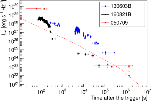
Figure 6: The observed luminosity density lightcurves at 5 keV for SGRBs 050709, 130603B and 160821B that have kilonova association. The red dashed line represents the afterglow model for GRB 050709 with $\varepsilon_{\rm e}$ = 0.1, $\varepsilon_{B}$ = 0.05, and $n_{\rm ISM}$ = 10^-2 cm^-3.

5 Conclusion

We report the possible evidence of soft X-ray emission right after the prompt hard-spike emission from GRB 050709, which may be interpreted as cocoon emission. The cocoon emission is tightly coupled to the jet physics of GRBs. Hence, assuming radiation dominant cocoon we estimated the properties of the cocoon of GRB 050709 at the breakout time such as the cocoon radius as $\sim$10⁹ cm and the cocoon pressure as $\sim$10¹⁹ erg cm^-3. These results are consistent with the cocoon model with injected thermal energy of $\sim$$10^{46}\mathrm{erg}$ given by the previous numerical studies in the narrow-jet scenario (Hamidani et al., 2021). We also compared the results of GRB 050709 to those of other short GRBs, specifically GRBs 170817A and 150101B, which exhibited similar light curves (i.e., hard-spike and soft-tail components). Our analysis indicates that the cocoon pressure and temperature for GRB 050709 are relatively higher than those observed in the other two GRBs. This difference may suggest that GRB 050709 had an on-axis jet compared to the other two GRBs. The viewing angle provides crucial information to understand GRB brightness, intrinsic rate, jet structure (Ioka & Nakamura, 2001; Yamazaki et al., 2002, 2004; Eichler, 2017; Ioka & Nakamura, 2018; Eichler, 2018; Matsumoto et al., 2019; Ioka et al., 2019; Fraija et al., 2019; Takahashi & Ioka, 2021) and muti-wavelength afterglow lightcurves (e.g., Troja et al. (2018a, b); Fong et al. (2019); Troja et al. (2019b); Lamb et al. (2020); Fraija et al. (2022)), along with details on kilonova characteristics because the viewing angle may also contribute to explaining the observed complex behavior of the kilonova emission from GW 170817 (e.g., Tanaka et al. (2017); Kawaguchi et al. (2020)).

The soft tail emission, as discussed in the paper, was predominantly observed below $\sim$10 keV, as seen in Fig. 1. If this holds for other SGRBs, current observatories such as Fermi-GBM and Swift-BAT face challenges in effectively covering this soft X-ray band. The future gamma-ray burst mission, HiZ-GUNDAM (Yonetoku et al., 2020), scheduled for the 2030s, is expected to advance capabilities in detecting electromagnetic emission from SGRBs: the wide-field X-ray monitors will be able to detect soft X-ray emission in the prompt and extended emission phases, and the near infrared telescope will conduct the follow-up observations of early afterglow or kilonova emission, which makes this mission very unique.

This study was supported by JSPS KAKENHI Grant Numbers JP22J12717 (N.O.), JP17H06362 (M.A.), JP23H04898 (D.Y. and M.A.), JP23H04895 (T.S.), the CHOZEN Project of Kanazawa University (D.Y., M.A., and T.S.), and the JSPS Leading Initiative for Excellent Young Researchers Program (M.A.).

References

- Abbott et al. (2017a) Abbott, B. P., et al. 2017a, Phys. Rev. Lett., 119, 161101
- Abbott et al. (2017b) —. 2017b, ApJ, 848, L13
- Alexander et al. (2018) Alexander, K., , et al. 2018, ApJ, 863, L18
- Arcavi et al. (2017) Arcavi, I., McCully, C., Hosseinzadeh, G., et al. 2017, ApJ, 848, L33, 10.3847/2041-8213/aa910f
- Arimoto et al. (2016) Arimoto, M., et al. 2016, ApJ, 833, 139, 10.3847/1538-4357/833/2/139
- Arnaud et al. (2011) Arnaud, K., et al. 2011, Handbook of X-ray Astronomy
- Arnaud (1996) Arnaud, K. A. 1996, in \asp, Vol. 101, Astronomical Data Analysis Software and Systems V, ed. G. H. Jacoby & J. Barnes, 17
- Atteia et al. (2003) Atteia, J.-L., et al. 2003, \aip, 662, 17
- Barkov & Pozanenko (2011) Barkov, M. V., & Pozanenko, A. S. 2011, MNRAS, 417, 2161, 10.1111/j.1365-2966.2011.19398.x
- Biltzinger et al. (2020) Biltzinger, B., et al. 2020, A&A, 640, A8
- Bucciantini et al. (2012) Bucciantini, N., et al. 2012, MNRAS, 419, 1537, 10.1111/j.1365-2966.2011.19810.x
- Burns et al. (2018) Burns, E., et al. 2018, ApJ, 863, L34
- Chornock et al. (2017) Chornock, R., Berger, E., Kasen, D., et al. 2017, ApJ, 848, L19, 10.3847/2041-8213/aa905c
- Coulter et al. (2017) Coulter, D., et al. 2017, Science, 358, 1556
- Covino et al. (2006) Covino, S., et al. 2006, A&A, 447, L5, 10.1051/0004-6361:200500228
- D’Avanzo et al. (2018) D’Avanzo, P., et al. 2018, A&A, 613, L1, 10.1051/0004-6361/201832664
- de Ugarte Postigo et al. (2014) de Ugarte Postigo, A., et al. 2014, A&A, 563, A62, 10.1051/0004-6361/201322985
- Díaz et al. (2017) Díaz, M. C., Macri, L. M., Garcia Lambas, D., et al. 2017, ApJ, 848, L29, 10.3847/2041-8213/aa9060
- Dobie et al. (2018) Dobie, D., et al. 2018, ApJ, 858, L15, 10.3847/2041-8213/aac105
- Drout et al. (2017) Drout, M. R., Piro, A. L., Shappee, B. J., et al. 2017, Science, 358, 1570, 10.1126/science.aaq0049
- D’Avanzo et al. (2018) D’Avanzo, P., et al. 2018, A&A, 613, L1
- Eichler (2017) Eichler, D. 2017, ApJ, 851, L32, 10.3847/2041-8213/aa9aec
- Eichler (2018) —. 2018, ApJ, 869, L4, 10.3847/2041-8213/aaec0d
- Fong et al. (2019) Fong, W., et al. 2019, ApJ, 883, L1, 10.3847/2041-8213/ab3d9e
- Fong et al. (2016) Fong, W.-f., et al. 2016, ApJ, 833, 151
- Fox et al. (2005) Fox, D. B., et al. 2005, Nature, 437, 845
- Fraija et al. (2022) Fraija, N., Galvan-Gamez, A., Betancourt Kamenetskaia, B., et al. 2022, ApJ, 940, 189, 10.3847/1538-4357/ac68e1
- Fraija et al. (2019) Fraija, N., Lopez-Camara, D., Pedreira, A. C. C. d. E. S., et al. 2019, ApJ, 884, 71, 10.3847/1538-4357/ab40a9
- Ghirlanda et al. (2019) Ghirlanda, G., Salafia, O. S., Paragi, Z., et al. 2019, Science, 363, 968, 10.1126/science.aau8815
- Gill & Granot (2018) Gill, R., & Granot, J. 2018, MNRAS, 478, 4128, 10.1093/mnras/sty1214
- Goldstein et al. (2017) Goldstein, A., et al. 2017, ApJ, 848, L14
- Golkhou & Butler (2014) Golkhou, V. Z., & Butler, N. R. 2014, ApJ, 787, 90, 10.1088/0004-637X/787/1/90
- Gottlieb et al. (2018) Gottlieb, O., et al. 2018, MNRAS, 479, 588, 10.1093/mnras/sty1462
- Granot et al. (2018) Granot, J., et al. 2018, MNRAS, 481, 2711, 10.1093/mnras/sty2454
- Haggard et al. (2017) Haggard, D., et al. 2017, ApJ, 848, L25, 10.3847/2041-8213/aa8ede
- Hajela et al. (2019) Hajela, A., et al. 2019, ApJ, 886, L17, 10.3847/2041-8213/ab5226
- Hajela et al. (2022) —. 2022, ApJ, 927, L17, 10.3847/2041-8213/ac504a
- Hamidani & Ioka (2023a) Hamidani, H., & Ioka, K. 2023a, MNRAS, 520, 1111, 10.1093/mnras/stad041
- Hamidani & Ioka (2023b) —. 2023b, MNRAS, 524, 4841, 10.1093/mnras/stad1933
- Hamidani et al. (2024) Hamidani, H., Kimura, S. S., Tanaka, M., & Ioka, K. 2024, ApJ, 963, 137, 10.3847/1538-4357/ad20d0
- Hamidani et al. (2020) Hamidani, H., et al. 2020, MNRAS, 491, 3192, 10.1093/mnras/stz3231
- Hamidani et al. (2021) Hamidani, H., et al. 2021, MNRAS, 500, 627
- Ioka & Nakamura (2001) Ioka, K., & Nakamura, T. 2001, ApJ, 554, L163, 10.1086/321717
- Ioka & Nakamura (2018) —. 2018, Progress of Theoretical and Experimental Physics, 2018, 043E02, 10.1093/ptep/pty036
- Ioka et al. (2019) Ioka, K., et al. 2019, MNRAS, 487, 4884
- Jin et al. (2016) Jin, Z.-P., et al. 2016, Nat. Commun., 7, 1
- Kagawa et al. (2015) Kagawa, Y., et al. 2015, ApJ, 811, 4
- Kagawa et al. (2019) Kagawa, Y., et al. 2019, ApJ, 877, 147, 10.3847/1538-4357/ab1bd6
- Kasliwal et al. (2017) Kasliwal, M., et al. 2017, Science, 358, 1559
- Kasliwal et al. (2017) Kasliwal, M. M., et al. 2017, ApJ, 843, L34, 10.3847/2041-8213/aa799d
- Kawaguchi et al. (2020) Kawaguchi, K., Shibata, M., & Tanaka, M. 2020, ApJ, 889, 171, 10.3847/1538-4357/ab61f6
- Kilpatrick et al. (2017) Kilpatrick, C. D., Foley, R. J., Kasen, D., et al. 2017, Science, 358, 1583, 10.1126/science.aaq0073
- Kimura et al. (2019) Kimura, S. S., et al. 2019, ApJ, 887, L16, 10.3847/2041-8213/ab59e1
- Lamb et al. (2019) Lamb, G., et al. 2019, ApJ, 870, L15
- Lamb et al. (2020) Lamb, G. P., Levan, A. J., & Tanvir, N. R. 2020, ApJ, 899, 105, 10.3847/1538-4357/aba75a
- Lamb et al. (2019a) Lamb, G. P., et al. 2019a, ApJ, 870, L15, 10.3847/2041-8213/aaf96b
- Lamb et al. (2019b) Lamb, G. P., Tanvir, N. R., Levan, A. J., et al. 2019b, ApJ, 883, 48, 10.3847/1538-4357/ab38bb
- Lazzati et al. (2017a) Lazzati, D., et al. 2017a, MNRAS, 471, 1652, 10.1093/mnras/stx1683
- Lazzati et al. (2017b) —. 2017b, ApJ, 848, L6, 10.3847/2041-8213/aa8f3d
- Lazzati et al. (2018) —. 2018, Phys. Rev. Lett., 120, 241103, 10.1103/PhysRevLett.120.241103
- Levan et al. (2016) Levan, A. J., et al. 2016, GRB Coordinates Network, 19846, 1
- Lyman et al. (2018) Lyman, J. D., et al. 2018, Nature Astronomy, 2, 751, 10.1038/s41550-018-0511-3
- MacLachlan et al. (2013) MacLachlan, G., et al. 2013, MNRAS, 432, 857
- Margutti et al. (2017) Margutti, R., et al. 2017, ApJ, 848, L20, 10.3847/2041-8213/aa9057
- Margutti et al. (2018) —. 2018, ApJ, 856, L18, 10.3847/2041-8213/aab2ad
- Matsumoto et al. (2019) Matsumoto, T., Nakar, E., & Piran, T. 2019, MNRAS, 486, 1563, 10.1093/mnras/stz923
- Meegan et al. (2009) Meegan, C., Lichti, G., Bhat, P. N., et al. 2009, ApJ, 702, 791, 10.1088/0004-637X/702/1/791
- Mészáros & Rees (2000) Mészáros, P., & Rees, M. J. 2000, ApJ, 530, 292, 10.1086/308371
- Metzger et al. (1974) Metzger, A. E., Parker, R. H., Gilman, D., Peterson, L. E., & Trombka, J. I. 1974, ApJ, 194, L19, 10.1086/181660
- Metzger et al. (2008) Metzger, B. D., et al. 2008, MNRAS, 385, 1455, 10.1111/j.1365-2966.2008.12923.x
- Mooley et al. (2018) Mooley, K., et al. 2018, Nature, 561, 355
- Nakamura et al. (2014) Nakamura, T., et al. 2014, ApJ, 796, 13, 10.1088/0004-637X/796/1/13
- Nakar & Piran (2017) Nakar, E., & Piran, T. 2017, ApJ, 834, 28, 10.3847/1538-4357/834/1/28
- Nakar et al. (2018) Nakar, E., et al. 2018, ApJ, 867, 18, 10.3847/1538-4357/aae205
- Nemiroff et al. (1997) Nemiroff, R. J., et al. 1997, J. Geophys. Res., 102, 9659
- Nicholl et al. (2017) Nicholl, M., Berger, E., Kasen, D., et al. 2017, ApJ, 848, L18, 10.3847/2041-8213/aa9029
- Norris et al. (2006) Norris, J. P., et al. 2006, ApJ, 643, 266
- Pe’er et al. (2006) Pe’er, A., et al. 2006, ApJ, 652, 482, 10.1086/507595
- Pian et al. (2017) Pian, E., D’Avanzo, P., Benetti, S., et al. 2017, Nature, 551, 67, 10.1038/nature24298
- Piran (2005) Piran, T. 2005, Reviews of Modern Physics, 76, 1143
- Piro & Kollmeier (2018) Piro, A. L., & Kollmeier, J. A. 2018, ApJ, 855, 103, 10.3847/1538-4357/aaaab3
- Resmi et al. (2018) Resmi, L., et al. 2018, ApJ, 867, 57
- Ricker et al. (2003) Ricker, G., et al. 2003, \aip, 662, 3
- Ryan et al. (2020) Ryan, G., et al. 2020, ApJ, 896, 166, 10.3847/1538-4357/ab93cf
- Ryde et al. (2010) Ryde, F., et al. 2010, ApJ, 709, L172, 10.1088/2041-8205/709/2/L172
- Savchenko et al. (2017) Savchenko, V., et al. 2017, ApJ, 848, L15
- Schmidt (1978) Schmidt, W. K. H. 1978, Nature, 271, 525
- Shappee et al. (2017) Shappee, B. J., Simon, J. D., Drout, M. R., et al. 2017, Science, 358, 1574, 10.1126/science.aaq0186
- Shirasaki et al. (2003) Shirasaki, Y., et al. 2003, PASJ, 55, 1033
- Smartt et al. (2017) Smartt, S. J., Chen, T. W., Jerkstrand, A., et al. 2017, Nature, 551, 75, 10.1038/nature24303
- Soares-Santos et al. (2017) Soares-Santos, M., Holz, D. E., Annis, J., et al. 2017, ApJ, 848, L16, 10.3847/2041-8213/aa9059
- Takahashi & Ioka (2021) Takahashi, K., & Ioka, K. 2021, MNRAS, 501, 5746, 10.1093/mnras/stab032
- Tanaka et al. (2017) Tanaka, M., et al. 2017, PASJ, 69, 102, 10.1093/pasj/psx121
- Tanvir et al. (2013) Tanvir, N. R., et al. 2013, Nature, 500, 547, 10.1038/nature12505
- Troja et al. (2017) Troja, E., et al. 2017, Nature, 551, 71, 10.1038/nature24290
- Troja et al. (2018) —. 2018, Nature Communications, 9, 4089, 10.1038/s41467-018-06558-7
- Troja et al. (2018a) Troja, E., et al. 2018a, MNRAS, 478, L18
- Troja et al. (2018b) —. 2018b, Nat. Commun., 9, 1
- Troja et al. (2019a) Troja, E., van Eerten, H., Ryan, G., et al. 2019a, MNRAS, 489, 1919, 10.1093/mnras/stz2248
- Troja et al. (2019b) Troja, E., et al. 2019b, MNRAS, 489, 2104, 10.1093/mnras/stz2255
- Troja et al. (2020) —. 2020, MNRAS, 498, 5643, 10.1093/mnras/staa2626
- Troja et al. (2022) —. 2022, MNRAS, 510, 1902, 10.1093/mnras/stab3533
- Utsumi et al. (2017) Utsumi, Y., Tanaka, M., Tominaga, N., et al. 2017, PASJ, 69, 101, 10.1093/pasj/psx118
- Valenti et al. (2017) Valenti, S., Sand, D. J., Yang, S., et al. 2017, ApJ, 848, L24, 10.3847/2041-8213/aa8edf
- Villasenor et al. (2005) Villasenor, J., et al. 2005, Nature, 437, 855
- von Kienlin et al. (2019) von Kienlin, A., et al. 2019, ApJ, 876, 89, 10.3847/1538-4357/ab10d8
- Wu & MacFadyen (2019) Wu, Y., & MacFadyen, A. 2019, ApJ, 880, L23, 10.3847/2041-8213/ab2fd4
- Yamazaki et al. (2002) Yamazaki, R., Ioka, K., & Nakamura, T. 2002, ApJ, 571, L31, 10.1086/341225
- Yamazaki et al. (2004) —. 2004, ApJ, 607, L103, 10.1086/421872
- Yonetoku et al. (2020) Yonetoku, D., et al. 2020, in Proc. SPIE, Vol. 11444, Space Telescopes and Instrumentation 2020: Ultraviolet to Gamma Ray, 114442Z, 10.1117/12.2560603