Convergence Analysis of Flow Matching in Latent Space with Transformers

Abstract

We present theoretical convergence guarantees for ODE-based generative models, specifically flow matching. We use a pre-trained autoencoder network to map high-dimensional original inputs to a low-dimensional latent space, where a transformer network is trained to predict the velocity field of the transformation from a standard normal distribution to the target latent distribution. Our error analysis demonstrates the effectiveness of this approach, showing that the distribution of samples generated via estimated ODE flow converges to the target distribution in the Wasserstein-2 distance under mild and practical assumptions. Furthermore, we show that arbitrary smooth functions can be effectively approximated by transformer networks with Lipschitz continuity, which may be of independent interest.

Keywords: deep generative model, ODE flow, transformer network, end-to-end error bound

1 Introduction

A wide variety of statistics and machine learning problems can be framed as generative modeling, especially when there is an emphasis on accurately modeling and efficiently sampling from intricate distributions, including those associated with images, sound, and text. The essence of generative modeling lies in its ability to learn a target distribution from finite samples, a task at which models incorporating deep neural networks have recently achieved considerable success.

Generative Adversarial Networks (GANs; goodfellow2014generative; arjovsky2017wasserstein), as a flagship example of deep generative models, have successfully been applied to a wide range of application challenges, including the synthesis of photorealistic images and videos (radford2015unsupervised; wang2018high; chan2019everybody), data augmentation (frid2018synthetic), style transfer (zhu2017unpaired), and facial editing (karras2019style). Additionally, significant research has been conducted to analyze the theoretical properties of GANs. bai2018approximability demonstrated that GANs could learn distributions within the Wasserstein distance, provided the discriminator class has sufficient distinguishing capability against the generator class. chen2020statistical established a minimax optimal convergence rate based on optimal transport theory, which necessitates the input and output dimensions of the generator to be identical. huang2022error proved that GANs could learn any distribution with bounded support. Despite their theoretical elegance and practical achievements, GANs often encounter challenges such as training instability, mode collapse, and difficulties in evaluating the quality of generated data.

The recent breakthrough known as the diffusion model has gained notable attention for its superior sample quality and a significantly more stable and controllable training process compared to GANs. The initial concept of the diffusion model involves training a denoising model to progressively transform noise data into samples that adhere to the target distribution (ho2020denoising), which has soon been mathematically proven to correspond to learning either the drift term of a Stochastic Differential Equation (SDE) or the velocity field of an Ordinary Differential Equation (ODE) (song2021scorebased). In SDE-based methods, the target data density degenerates into a simpler Gaussian density through the Ornstein-Uhlenbeck (OU) process, followed by solving a reverse-time SDE to generate samples from noise (ho2020denoising; song2021scorebased; meng2021sdedit). Researchers have also proposed the diffusion Schrödinger Bridge (SB), which formulates a finite-time SDE, effectively accelerating the simulation time (de2021diffusion). The achievements of ODE-based methods are equally remarkable, with most adopting an approach involving interpolative trajectory modeling (liu2022flow; albergo2022building; liu2023flowgrad; xu2022poisson). liu2022flow employs linear interpolation to connect the target distribution with a reference distribution, while albergo2022building extends this interpolation to nonlinear cases. Further gao2023gaussian uses interpolation to analyze the regularity of a broad class of ODE flows.

In the past few years, there has been an explosive development in SDE/ODE-based generative models, with many models showcasing outstanding performance across a diverse array of application challenges. dhariwal2021diffusion have demonstrated that diffusion models outperform GANs in both unconditional and conditional image synthesis, setting a new benchmark in the quality of generated images. rombach2022high showed that generative processes operating in a latent space can significantly reduce computational resources while maintaining high-quality text-to-image generation. A line of research (kong2020diffwave; chen2020wavegrad; popov2021grad; liu2022diffsinger) introduced versatile diffusion models capable of synthesizing high-fidelity audio, marking considerable progress in the quality of speech and music generation. Additionally, considerable research has concentrated on text-to-video generation, aiming to create long videos while maintaining high visual quality and adherence to the user’s prompt (blattmann2023stable; blattmann2023align; wu2023tune; chen2024videocrafter2; wang2024videocomposer; videoworldsimulators2024). Despite these models being tailored for various tasks, they typically share two common features. Firstly, they utilize an encoder-decoder architecture to map high-dimensional original inputs to a low-dimensional latent space, where the SDE/ODE-based generative process takes place. Secondly, they employ transformers as the backbone architecture.

Although some analyses have attempted to explain the success of SDE/ODE-based generative models, these analyses either involve technical and unverifiable assumptions or do not align with the models actually used in practice. In a series of studies (lee2022convergence; lee2023convergence; de2022convergence; chen2022sampling; chen2023improved; benton2023linear; conforti2023score), researchers systematically examined the sampling errors of diffusion models across various target distributions and have determined the optimal sampling error order. Their analysis assumes that the velocity field or drift term in diffusion models has been well-trained, without considering the training process and model selection, thus not providing an end-to-end analysis. It should be noted that end-to-end error analysis is rarely observed even in the domain of general ODE/SDE generative methods. To our knowledge, wang2021deep first proved the consistency of the Schrödinger Bridge approach through an end-to-end analysis. oko2023diffusion proved that in an SDE-based generative model, when the true density function has certain regularities and the empirical score matching loss is properly minimized, the generated data distribution achieves nearly minimax optimal estimation rates in total variation distance and Wasserstein-1 distance. tang2024adaptivity further extended the analysis to the intrinsic manifold assumption. chen2023score considered a special case in which the encoder and decoder are linear models. chang2024deep developed an ODE-based framework and derived a non-asymptotic convergence rate in the Wasserstein-2 distance. However, these analyses do not consider the transformer architecture or incorporate pre-training, which are commonly used in practical implementations, leaving a gap in explaining the success of SDE/ODE-based generative models.

In this paper, we mathematically prove that the distribution of the samples generated via ODE flow converges to the target distribution in the Wasserstein-2 distance under mild and practical assumptions, providing the first comprehensive end-to-end error analysis that considers the transformer architecture and allows for domain shift in pre-training.

1.1 Our main contributions

Our main contributions are summarized as follows.

• We establish approximation guarantees for transformer networks subject to Lipschitz continuity constraints, which may be of independent interest. (Theorem LABEL:theorem:_app_3 and LABEL:corollary:_app_1). Specifically, we prove that the transformer network can approximate any function, with the Lipschitz continuity of the network remaining independent of the approximation error. Under the assumption that the target distribution has bounded support, we show that the ground truth velocity field is a smooth function, allowing it to be sufficiently approximated by a properly chosen transformer network.

• We establish statistical guarantees for pre-training using the learned encoder and decoder network (Lemma LABEL:lemma:_ae_rate). Choosing transformer networks as our encoder and decoder, we show that the excessive risk of reconstruction loss converges at a rate of $\widetilde{\mathcal{O}}(m^{-\frac{1}{D+2}})$, where $m$ is the pre-training sample size, only under the assumptions that the pre-trained data distribution has bounded support and that there exist smooth functions minimizing the reconstruction loss.

• We establish estimation guarantees for the target distribution using the estimated velocity field (Theorem LABEL:theorem:_main_result). By choosing proper discretization step size and early stopping time for generating samples, we prove that $\mathbb{E}_{\mathcal{Y},\mathcal{X}}[W_{2}(\widehat{\gamma}_{T},\gamma_{1})]=\mathcal{O}(\sqrt{\varepsilon_{\widetilde{\gamma}_{1}}}+\varepsilon_{\widetilde{\gamma}_{1},\gamma_{1}})$, where $\widehat{\gamma}_{T}$ is the generated data distribution, $\gamma_{1}$ is the target distribution, $\varepsilon_{\widetilde{\gamma}_{1},\gamma_{1}}$ denotes the domain shift between the target distribution and the pre-trained data distribution, and $\varepsilon_{\widetilde{\gamma}_{1}}$ is the minimum reconstruction loss achievable by the encoder-decoder architecture. Specifically, if there is no domain shift and the encoder-decoder architecture can perfectly reconstruct the distribution, our results show that the generated data distribution converges to the target distribution in Wasserstein-2 distance.

1.2 Organization

The rest of the paper is organized as follows. In Section 2, we provide notations and introduce key concepts. In Section LABEL:sec:_approximation, we show that the true velocity field can be well approximated by a Lipschitz transformer network. In Section LABEL:sec:_generalization_and_sampling, we show that the true velocity field can be efficiently estimated, and analyze the error of distribution recovery using the estimated velocity field. Finally, in Section LABEL:sec:_end-to-end_error, we analyze the error introduced by the pre-trained autoencoder.

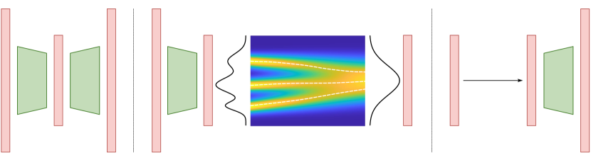
at (0,0) ; at (-6.8,-0.05) $\widehat{\boldsymbol{E}}$; at (-5.44,-0.05) $\widehat{\boldsymbol{D}}$; at (-2.93,-0.05) $\widehat{\boldsymbol{E}}$; at (6.75,-0.05) $\widehat{\boldsymbol{D}}$; at (5.08,0.4) Euler; at (5.08,0.1) method; at (-6.12,-2.4) Pre-training; at (-0.25,-2.4) Flow matching; at (5.57,-2.4) Sampling;

Figure 1: An illustration of our framework. Pre-training: Based on $m$ samples $\mathcal{Y}=\{\boldsymbol{y}_{i}\}_{i=1}^{m}$ drawn i.i.d. from pre-trained data distribution $\widetilde{\gamma}_{1}$, we minimize the empirical reconstruction loss to obtain an encoder $\widehat{\boldsymbol{E}}:[0,1]^{D}\rightarrow[0,1]^{d}$ and the corresponding decoder $\widehat{\boldsymbol{D}}:[0,1]^{d}\rightarrow\mathbb{R}^{D}$. These will serve as the bridge linking the high-dimensional input space and the low-dimensional latent space. Flow matching: For the target distribution $\gamma_{1}$ and $n$ samples $\mathcal{X}=\{\boldsymbol{x}_{i}\}_{i=1}^{n}$ drawn from it, the encoder $\widehat{\boldsymbol{E}}$ maps them to the latent space with $\pi_{1}=\widehat{\boldsymbol{E}}_{\#}\gamma_{1}$ and $\widehat{\boldsymbol{E}}(\mathcal{X})=\{\widehat{\boldsymbol{E}}(\boldsymbol{x}_{i})\}_{i=1}^{n}$. Flow matching is then applied within the latent space, where a transformer network is trained to predict the velocity field of the transformation from a standard normal distribution $\pi_{0}=\mathcal{N}(0,I_{d})$ to the target latent distribution $\pi_{1}$. Sampling: Given the estimated velocity field, we can generate samples from an approximation of the continuous flow ODE starting from the prior distribution $\pi_{0}$. The generated latent data distribution $\widehat{\pi}_{T}$ will be mapped back to the high-dimensional space by the decoder $\widehat{\boldsymbol{D}}$, resulting in the generated data distribution $\widehat{\gamma}_{T}=\widehat{\boldsymbol{D}}_{\#}\widehat{\pi}_{T}$.

2 Preliminaries

In this section, we introduce the notations used throughout this paper. Additionally, we provide details about transformer networks, pre-training, and flow matching.

Notations. Here we summarize the notations. Given a real number $\alpha$, we denote $\lfloor\alpha\rfloor$ as the largest integer smaller than $\alpha$ (in particular, if $\alpha$ is an integer, $\lfloor\alpha\rfloor=\alpha-1)$. For a vector $\boldsymbol{x}\in\mathbb{R}^{d}$, we denote its $\ell^{2}$-norm by $\|\boldsymbol{x}\|$, the $\ell^{\infty}$-norm by $\|\boldsymbol{x}\|_{\infty}=\max_{i}|x_{i}|$. We define $\boldsymbol{x}^{\otimes 2}:=\boldsymbol{x}\boldsymbol{x}^{\top}$. We define the operator norm of a matrix $A$ as $\|A\|_{\text{op}}:=\sup_{\|\boldsymbol{x}\|\leq 1}\|A\boldsymbol{x}\|$. For two matrices $A,B\in\mathbb{R}^{d\times d}$, we say $A\preceq B$ if $B-A$ is positive semi-definite. We denote the identity matrix in $\mathbb{R}^{d\times d}$ by $I_{d}$. For a twice continuously differentiable function $f:\mathbb{R}^{d}\rightarrow\mathbb{R}$, let $\nabla f,\nabla^{2}f$, and $\Delta f$ denote its gradient, Hessian, and Laplacian, respectively. For a probability density function $\pi$ and a measurable function $f:\mathbb{R}^{d}\rightarrow\mathbb{R}$, we define the $L^{2}(\pi)$-norm of $f$ as $\|f\|_{L^{2}(\pi)}:=(\int(f(\boldsymbol{x}))^{2}\pi(\boldsymbol{x})\mathrm{d}\boldsymbol{x})^{1/2}$. We define $L^{\infty}(K)$-norm as $\|f\|_{L^{\infty}(K)}:=\sup_{\boldsymbol{x}\in K}|f(\boldsymbol{x})|$. The function composition operation is marked as $g\circ f:=g(f(x))$ for functions $f$ and $g$. We use the asymptotic notation $f(x)=\mathcal{O}(g(x))$ to denote the statement that $f(x)\leq Cg(x)$ for some constant $C>0$ and $\widetilde{\mathcal{O}}(\cdot)$ to ignore the logarithm. For a vector function $\boldsymbol{v}:\mathbb{R}^{d}\rightarrow\mathbb{R}^{d^{\prime}}$, we define its $L^{2}(\pi)$-norm as $\|\boldsymbol{v}\|_{L^{2}(\pi)}:=\|\|\boldsymbol{v}\|\|_{L^{2}(\pi)}$ and $L^{\infty}(K)$-norm as $\|\boldsymbol{v}\|_{L^{\infty}(K)}:=\|\|\boldsymbol{v}\|\|_{L^{\infty}(K)}$. For any dataset $\mathcal{D}=\{\boldsymbol{x}_{i}\}_{i=1}^{n}$, we define the image of $\mathcal{D}$ under $\boldsymbol{v}$ as $\boldsymbol{v}(\mathcal{D}):=\{\boldsymbol{v}(\boldsymbol{x}_{i})\}_{i=1}^{n}$. Given two distributions $\mu$ and $\nu$, the Wasserstein-2 distance is defined as $W_{2}(\mu,\nu):=\inf_{\pi\in\Pi(\mu,\nu)}\mathbb{E}_{(x,y)\sim\pi}[\|x-y\|^{2}]^{1/2}$, where $\Pi(\mu,\nu)$ is the set of all couplings of $\mu$ and $\nu$. A coupling is a joint distribution on $\mathbb{R}^{d}\times\mathbb{R}^{d}$ whose marginals are $\mu$ and $\nu$ on first and second factors, respectively. Let $\boldsymbol{f}:\mathbb{R}^{d}\rightarrow\mathbb{R}^{d^{\prime}}$ be a measurable mapping and $\mu$ be a probability measure on $\mathbb{R}^{d}$. The push-forward measure $\boldsymbol{f}_{\#}\mu$ of a measurable set $K$ is defined as $\boldsymbol{f}_{\#}\mu:=\mu(\boldsymbol{f}^{-1}(K))$. In neural networks, the Rectified Linear Unit (ReLU) activation function is denoted by $\sigma(x)=\max\{x,0\}$ and is applied element-wise to vectors or matrices. We define the hardmax operator as $\sigma_{H}(\boldsymbol{x}):=\lim_{c\rightarrow+\infty}\exp(c\boldsymbol{x})/\|\exp(c\boldsymbol{x})\|_{1}$, where the operation is performed column-wise if the input to $\sigma_{H}$ is a matrix. The Hadamard product $\odot$ refers to the element-wise multiplication of two vectors or matrices of the same dimensions.

2.1 Transformer networks

In the last few years, academic inquiry has concentrated on the approximation power and generalization capability of ReLU neural networks (yarotsky2017error; suzuki2018adaptivity; bartlett2019nearly; yarotsky2020phase; schmidt2020nonparametric; lu2021deep; shen2022optimal). These networks become the preferred choice for theoretical analysis and are able to achieve the minimax optimal rate in many problems (huang2022error; duan2022convergence; jiao2023deep; oko2023diffusion; liu2024deep). In contrast, the theoretical understanding of transformer networks remains limited, despite their resounding success in practical applications. gurevych2022rate recently provided a framework to study the approximation properties and generalization abilities of transformer networks. We adopt their framework and extend it by incorporating control over the regularity of the neural network functions.

Given $d,d^{\prime}\in\mathbb{N}$, we define a transformer network $\boldsymbol{\phi}:\mathbb{R}^{d}\rightarrow\mathbb{R}^{d^{\prime}}$ as follows: ϕ=E_out ∘F_N^(FF) ∘F_N^(SA) ∘⋯∘F_1^(FF) ∘F_1^(SA) ∘E_in ∘P.

The first layer of the transformer network $P$, known as ”patchify”, divides the spatial input into patches. Namely, an input $\boldsymbol{x}$ of dimension $d$ is transformed into a sequence $X$ of $l$ tokens, where each token has a dimension of $d_{patch}$. These tokens are explicitly selected from components of the input, thus this layer does not require training. For simplicity, we assume $d=d_{patch}\times l$.

The input embedding layer $E_{in}:\mathbb{R}^{(d_{patch}+l)\times l}\rightarrow\mathbb{R}^{d_{model}\times l}$, incorporating position encoding, is a token-wise linear mapping: Z_0 =E_in(Concat( XI_l ))= A_in ( XI_l ) +b_in 1_l^⊤ where $A_{in}\in\mathbb{R}^{d_{model}\times(d_{patch}+l)}$ and $\boldsymbol{b}_{in}\in\mathbb{R}^{d_{model}}$ represent the weight matrix and bias vector of the embedding layer, and $\mathbbm{1}_{l}$ denotes a vector of $l$ components, each of which is 1.

The multi-head attention layer $F^{(SA)}:\mathbb{R}^{d_{model}\times l}\rightarrow\mathbb{R}^{d_{model}\times l}$ represents the interaction among tokens: F^(SA)(Z) = Z + ∑_s=1^h W_O,s(W_V,s Z) [((W_K,s Z)^⊤(W_Q,s Z)) ⊙σ_H((W_K,s Z)^⊤(W_Q,s Z))] where $h\in\mathbb{N}$ is the number of heads which we compute in parallel, $d_{k}\in\mathbb{N}$ is the dimension of the queries and keys, $d_{v}\in\mathbb{N}$ is the dimension of the values, $d_{model}=h\cdot d_{v}$, $W_{K,s},W_{Q,s}\in\mathbb{R}^{d_{k}\times d_{model}},W_{V,s}\in\mathbb{R}^{d_{v}\times d_{model}}$ and $W_{O,s}\in\mathbb{R}^{d_{model}\times d_{v}}$ are the weight matrices, and $\sigma_{H}$ is the hardmax operator. We include a skip-connection in the attention layer.

The token-wise feedforward neural network $F^{(FF)}:\mathbb{R}^{d_{model}\times l}\rightarrow\mathbb{R}^{d_{model}\times l}$ processes each token independently in parallel by applying two feedforward layers: F^(FF)(Y) = Y + W_2σ(W_1 Y + b_1 1_l^⊤) + b_21_l^⊤ where $d_{ff}\in\mathbb{N}$ denotes the hidden layer size of the feedforward layer, $W_{1}\in\mathbb{R}^{d_{ff}\times d_{model}},\boldsymbol{b}_{1}\in\mathbb{R}^{d_{ff}},W_{2}\in\mathbb{R}^{d_{model}\times d_{ff}}$ and $\boldsymbol{b}_{2}\in\mathbb{R}^{d_{model}}$ are parameters, and $\sigma$ is the ReLU activation function. The feedforward layer also includes a skip-connection.

The output embedding $E_{out}:\mathbb{R}^{d_{model}\times l}\rightarrow\mathbb{R}^{d^{\prime}}$, E_out(Z) = A_out z_1 + b_out where $Z=(\boldsymbol{z}_{1},\boldsymbol{z}_{2},\ldots,\boldsymbol{z}_{l})$, and $A_{out}\in\mathbb{R}^{d^{\prime}\times d_{model}}$ and $\boldsymbol{b}_{out}\in\mathbb{R}^{d^{\prime}}$ are the weight matrix and bias vector. It is important to highlight that only the first column of $Z$, specifically the first token, is used.

Based on the definitions provided, we configure the transformer networks as follows: T_d,d^′ (N, h, d_k, d_v, d_f f, B, J, γ) = { & ϕ: R^d →R^d^′ : ϕ in the form of (2.1), sup_x∥ϕ(x)∥ ≤B,
∥ϕ(x_1)-ϕ(x_2)∥ ≤γ∥x_1-x_2∥ for x_1, x_2 ∈[0,1]^d,
∑_r=1^N ∑_s=1^h (∥W_Q, r, s∥_0+ ∥W_K, r, s∥_0+∥W_V, r, s∥_0+ ∥W_O, r, s∥_0)
+∑_r=1^N (∥W_r, 1∥_0+∥b_r, 1∥_0+∥W_r, 2∥_0+∥b_r, 2∥_0)
+ ∥A_in∥_0+∥b_in∥_0 + ∥A_out∥