An implementation of nuclear many-body wave functions by the superposition of localized Gaussians

Abstract

We introduce a new framework for the low-energy nuclear structure calculations, which describes the single-particle wave function as a superposition of localized Gaussians. It is a hybrid of the Hartree-Fock and antisymmetrized molecular dynamics models. In the numerical calculations of oxygen, calcium isotopes and ${}^{100}{\rm Sn}$, the framework shows its potential by significantly improving upon AMD and yielding the results consistent with or even better than Hartree-Fock(-Bogoliubov) calculations based on harmonic oscillator expansions. In addition to the basic equations, general form of the matrix elements are also given.

xxxx, xxx

1 Introduction

The nuclear many body calculations often employ density functional with local density approximation or finite-range terms. The latter offer the advantage of not only better simulating the realistic properties of nuclear forces but also the potential to use interactions derived from first principles Feldmeier1998 ; Neff2003 ; Roth2005 ; Myo2015 ; Myo2017 ; Fukui2023 . To use finite-range interactions, the wave functions are usually expanded by basis functions which are tailored to the target problems minimizing computational costs. Most commonly used basis function is the harmonic oscillator (HO) basis including deformed one Gogny1975 ; Girod1983 ; Egido1980 ; Egido1995 ; Dobaczewski2004 . For a more accurate description of asymptotic forms of the wave functions, such as neutron halos, bases like transformed HO Stoitsov1998 ; Stoitsov2005 or Gaussian expansion Nakada2006 ; Nakada2008 are employed. In the time-dependent approaches, the Lagrange mesh method Hashimoto2013 has also been used. Each has its own advantages and disadvantages.

In this paper, we propose a framework which uses localized Gaussian (LG) wave packets as basis functions, and introduce its basic equations. LGs are characterized by 3-dimensional complex vectors representing their mean positions and momenta. By controlling them, a variety of nuclear structure and dynamics can be described. In particular, LGs have advantages in describing localized cluster structures Brink1965 ; Wildermuth1977 ; Saito1977 ; Horiuchi1977 ; Tohsaki1977 and reaction processes Kamimura1977 ; Saraceno1983 ; Caurier1982 ; Drozdz1982 . Moreover, they can efficiently describe systems with fewer bases making extensions to the beyond-mean-field framework relatively easier.

We show that the energy variation yields two sets of equations. The first one determines the positions and momenta of LGs, which naturally extends wave packet models such as microscopic cluster models, antisymmetrized molecular dynamics (AMD) Kanada-Enyo2003 ; Kanada-Enyo2012 ; Kimura2016 , and fermionic molecular dynamics (FMD) Feldmeier1990 ; Feldmeier1995 . The second determines the amplitudes of superposition which can be regarded as the Hartree-Fock equation determining the single-particle wave functions. Thus, this framework is a hybrid of the wave packet models and Hartree-Fock.

In addition to the formulation, we demonstrate simple numerical calculations using the Gogny D1S effective interaction Berger1991 to benchmark the new framework. We calculated the ground state of spherical nuclei, i.e., oxygen, and calcium isotopes, and compared with AMD and HFB with HO basis expansion Hilaire2007 . The new method improved AMD results, significantly in calcium isotopes. When pairing energy is negligible or not large, the new method gave equivalent or even better results compared to HF(B). The calculated proton and neutron density distributions revealed that wave functions were improved inside and outside the nucleus compared to AMD, particularly showing correct asymptotic behavior at large distances. As another example, we also present the results for ${}^{100}{\rm Sn}$. This nucleus is out of the applicability of ordinary AMD due to its larger mass number, but the present model also gave the reasonable results. By these examples, the new method showed its potential in studying various nuclear structure problems.

The paper is organized as follows. The next section introduces model wave function, its variational parameters and the formula for the energy variation of a simplified Hamiltonian. More general form of the Hamiltonian are discussed in the appendix. Section III demonstrates benchmark calculations for oxygen, calcium isotopes and ${}^{100}{\rm Sn}$. The last section summarizes this study.

2 Framework

2.1 Variational wave function

We employ a set of localized Gaussian (LG) basis functions to describe the single-particle wave functions. The LG is defined as,

$$\phi_{p}(\bm{r}) :=\braket{\bm{r}}{p}=\left(\frac{2\nu}{\pi}\right)^{3/4}\exp\Set{-\nu\left(\bm{r}-\frac{\bm{z}_{p}}{\sqrt{\nu}}\right)^{2}},$$ (1)

where $p$ (and $q,r,s,...$) is the index for the LGs, and $M$ is the number of the LGs which determines the size of the model space. The complex valued three-dimensional vector $\bm{z}_{p}$, which is the variational parameter, represents the average position and momentum of wave packet.

The single-particle wave function is expressed by a superposition of LGs,

$$\ket{i^{\alpha}}=\sum_{p=1}^{M}\ket{p}c^{\alpha}_{pi},\quad(i=1,...,Z\ {\rm or}\ N,\quad p=1,...,M),$$ (2)

where $\alpha$ denotes the isospin either proton or neutron, and $i$ (and $j,k,l,...$) is the index for the the particle with the isospin $\alpha$, which runs upto the proton or neutron number ($Z$ or $N$). $c^{\alpha}_{pi}$ is the two component spinor which is also determined by the energy variation. Thus, in this framework, the single-particle wave function has two different variational parameters, $\bm{z}_{p}$ and $c^{\alpha}_{pi}$.

Many-nucleon states composed of $Z$ protons and $N$ neutrons are expressed by an antisymmetrized product of the single-particle states, i.e., by Hartree-Fock approximation,

$$\ket{\Phi} =\mathcal{A}\bigl{[}\ket{1^{p}}\cdots\ket{Z^{p}}\ket{1^{n}}\cdots\ket{N^{n}}\bigr{]},$$ (3)

where $\ket{i^{p}}$ and $\ket{i^{n}}$ denote proton and neutron single-particle wave functions. As in the ordinary AMD for the structure calculations Kanada-Enyo2012 , one may extend the model wave function by employing the parity-projected and angular-momentum-projected ones,

$$\ket{\Phi^{\pi}} =\frac{1+\pi P_{x}}{2}\ket{\Phi},\quad(\pi=+\ \mathrm{or}\ -)$$ (4)

$$\ket{\Phi^{J\pi}_{MK}} =\frac{1+\pi P_{x}}{2}\int d\Omega D^{*}_{MK}(\Omega)R(\Omega)\ket{\Phi},$$ (5)

where $P_{x}$, $R(\Omega)$ and $D^{J}_{MK}(\Omega)$ denote the parity, rotation operators, and Wigner’s D function. The projection can be done before (PBV) or after (PAV) the energy variation.

Let us we compare the present model with others. Eq. (2) can be regarded as an extension of the AMD wave function. If $c^{\alpha}_{pi}$ is the Kronecker delta, i.e., $c^{\alpha}_{ip}=c^{\alpha}_{i}\delta_{p,\{\alpha,i\}}$, it reduces to the AMD wave function. We also note that Eq. (2) is similar to the AMD-HF Dote1997 and FMD Feldmeier1990 ; Feldmeier1995 wave functions, which also describe the single-particle wave functions by the superposition of LGs as,

$$\ket{i^{\alpha}} :=\sum_{p=1}^{M}\ket{pi^{\alpha}}c^{\alpha}_{pi},\quad(i=1,2,...,Z\ {\rm or}\ N),$$ (6)

$$\phi_{pi}^{\alpha}(\bm{r}) :=\braket{\bm{r}}{pi^{\alpha}}=\left(\frac{2\nu_{pi}^{\alpha}}{\pi}\right)^{3/4}\exp\biggl{\{}-\nu_{pi}^{\alpha}\Bigl{(}\bm{r}-\frac{\bm{z}_{pi}^{\alpha}}{\sqrt{\nu_{pi}^{\alpha}}}\Bigr{)}^{2}\biggr{\}}.$$ (7)

The difference between Eq. (2) and (6) lies in whether a LG is associated with a specific single-particle wave function or not, that is, whether the LG depends on the particle index $i$ or not. For instance, Eq. (2) uses a LG to describe both protons and neutrons, whereas AMD-HF and FMD do not. Hence, the present model more efficiently describes single-particle wave functions with smaller number of LGs. Furthermore, it can be easily extended to the quasi-particle states to handle the pairing correlations.

In relation with the Hartree-Fock framework, Eq. (2) is regarded as an implementation of Hartree-Fock by the basis expansion. However, note that the basis function $\ket{p}$ is variational through the parameter $\bm{z}_{p}$, while ordinary Hartree-Fock formulation employs fixed basis wave functions. Use of variational basis function enables the present model to describe various nuclear structures with fewer basis functions. Moreover, one can easily imagine its advantages when applied to a time-dependent problems.

2.2 Expectation value of the Hamiltonian

Here, we consider the application of this model to the nuclear structure problems. We wish to evaluate the expectation value of a Hamiltonian and obtain the optimal values of the variational parameters $\bm{z}_{p}$ and $c^{\alpha}_{ip}$ by the energy variation. For this purpose, we first introduce the overlap matrix and density matrix. The overlap matrix of LGs is defined as,

$$d_{pr} :=\braket{p}{r}=\exp\Set{-\frac{1}{2}(\bm{z}_{p}^{*}-\bm{z}_{r})^{2}}.$$ (8)

We also introduce the overlap matrix of the single-particle wave functions.

$$b^{\alpha}_{ik}:=\braket{i^{\alpha}}{k^{\alpha}}=\sum_{pr}d_{pr}\braket{c^{\alpha}_{pi}}{c^{\alpha}_{rk}}.$$ (9)

Note that the single-particle wave functions are unorthogonal. The density matrix is defined as in ordinary Hartree-Fock, but the inverse of the overlap matrix, $b^{-1}$, must be inserted due to the unorthogonality.

$$\rho^{\alpha}_{rp}:=\sum_{ik}\braket{c^{\alpha}_{pi}}{c^{\alpha}_{rk}}{b^{\alpha}}^{-1}_{ki},\quad\bm{\rho}^{\alpha}_{rp}:=\sum_{ik}\braket{c^{\alpha}_{pi}}{\bm{\sigma}}{c^{\alpha}_{rk}}{b^{\alpha}}^{-1}_{ki},$$ (10)

where $\bm{\rho}^{\alpha}$ has three component as $\bm{\rho}^{\alpha}=(\rho_{x}^{\alpha},\rho_{y}^{\alpha},\rho_{z}^{\alpha})$ corresponding to the $x,y,z$ components of the Pauli matrix $\bm{\sigma}$. It is convenient to introduce the bi-orthonormal spinors $\widetilde{c}$ and $\widetilde{\bm{c}}$,

$$\widetilde{c}^{\alpha}:=c^{\alpha}{b^{\alpha}}^{-1},\quad\widetilde{\bm{c}}^{\alpha}:=\bm{\sigma}\widetilde{c}^{\alpha}=\bm{\sigma}c^{\alpha}{b^{\alpha}}^{-1},$$ (11)

where (and in the following) we omit the index for particles ($i,j,...$) and LGs ($p,q,...$) and introduce the matrix notation for simplicity. This simplifies the expressions of the density matrix as,

$$\rho^{\alpha}=\widetilde{c}^{\alpha}{c^{\alpha\dagger}},\quad\bm{\rho}^{\alpha}=\widetilde{\bm{c}}^{\alpha}{c^{\alpha\dagger}}.$$ (12)

We also denote, in the following, the sum of the proton and neutron density matrices as,

$$\rho:=\rho^{p}+\rho^{n},\quad\bm{\rho}:=\bm{\rho}^{p}+\bm{\rho}^{n}.$$ (13)

Now, we consider the Hamiltonian composed of the kinetic energy and spin-isospin independent two-body interaction. More general cases are discussed in the appendix. Let us consider the one-body kinetic energy operator $T=\sum_{i=1}^{A}t_{i}$ with $t_{i}=-\hbar^{2}\nabla^{2}_{i}/2m$. Its matrix element by Eq. (3) is given as,

$$\braket{T}:=\frac{\braket{\Phi}{T}{\Phi}}{\braket{\Phi}{\Phi}}=\sum_{\alpha ik}\braket{i^{\alpha}}{t}{k^{\alpha}}{b^{\alpha}}^{-1}_{ki}=\sum_{pr}t_{pr}\rho_{rp},$$ (14)

where $t_{pr}$ is the matrix element of the kinetic energy calculated by LGs, i.e., $t_{pr}=\braket{p}{t}{r}$.

The matrix element of a spin-isospin independent two-body potential $V=\sum_{i<j}^{A}v_{ij}$ is given as,

$$\braket{V} :=\frac{\braket{\Phi}{V}{\Phi}}{\braket{\Phi}{\Phi}}=\frac{1}{2}\sum_{\alpha\beta ijkl}\set{\braket{i^{\alpha}j^{\beta}}{v|k^{\alpha}l^{\beta}}-\braket{i^{\alpha}j^{\beta}}{v}{l^{\beta}k^{\alpha}}}{b^{\alpha}}^{-1}_{ki}{b^{\beta}}^{-1}_{lj}$$

$$=\frac{1}{2}\sum_{pqrs}\sum_{\alpha\beta}\Set{\left(v_{pqrs}-\frac{1}{2}v_{pqsr}\right)\rho_{rp}^{\alpha}\rho_{sq}^{\beta}-\frac{1}{2}v_{pqsr}\bm{\rho}_{rp}^{\alpha}\cdot\bm{\rho}_{sq}^{\beta}},$$ (15)

where $v_{pqrs}$ is the non-antisymmetrized matrix element of the two-body potential defined by $v_{pqrs}=\braket{pq}{v}{rs}$, which is a functions of $\vec{z}^{*}_{p}$, $\vec{z}^{*}_{q}$, $\vec{z}_{r}$, and $\vec{z}_{s}$, but independent of the spinors, $c^{\alpha}_{pi}$. More general potentials can also be summarized in a similar form as presented in the appendix. By introducing the mean-field $\Gamma$, Eq. (15) is simplified as,

$$\braket{V} =\frac{1}{2}\sum_{pr}(\Gamma_{pr}\rho_{rp}+\bm{\Gamma}_{pr}\cdot\bm{\rho}_{rp}),$$ (16)

$$\Gamma_{pr} :=\sum_{sq}\left(v_{pqrs}-\frac{1}{2}v_{pqsr}\right)\rho_{sq},\quad\bm{\Gamma}_{pr}:=-\frac{1}{2}\sum_{sq}v_{pqsr}\bm{\rho}_{sq}.$$ (17)

From Eqs. (14) and (16), the expectation value of the Hamiltonian is given in a form analogous to the ordinary Hartree-Fock,

$$\braket{H} =\braket{T}+\braket{V}={\rm Tr}(t\rho)+\frac{1}{2}{\rm Tr}(\Gamma\rho+\bm{\Gamma}\cdot\bm{\rho}).$$ (18)

In the practical calculation with Gogny density functional, one also need to incorporate with the center-of-mass correction of the kinetic energy, spin-ispspin dependent and the density-dependent two-body interactions.

2.3 Energy variation

To determine the variational parameters $c^{\alpha}_{pi}$ and $\bm{z}_{p}$, we consider the stationary condition of the energy with respect to the variation of the wave function.

$$\delta\frac{\braket{\Phi}{H}{\Phi}}{\braket{\Phi}{\Phi}} =\sum_{pi\alpha}\delta c^{\alpha\dagger}_{pi}\left(\partial^{\alpha}_{pi}\frac{\braket{\Phi}{H}{\Phi}}{\braket{\Phi}{\Phi}}\right)+\sum_{p}\delta\vec{z}_{p}^{*}\cdot\left(\vec{\partial}_{p}\frac{\braket{\Phi}{H}{\Phi}}{\braket{\Phi}{\Phi}}\right)+h.c.=0,$$ (19)

where we shorthand $\partial/\partial\vec{z}^{*}_{p}$ and $\partial/\partial c^{\alpha\dagger}_{pi}$ as $\vec{\partial}_{p}$ and $\partial^{\alpha}_{pi}$, respectively. Note that we use notation of arrowed vector $\vec{z}_{p}$ to distinguish the vectors originate in the variation from others denoted by the bold fonts. From Eq. (19), we get the stationary condition for $c^{\alpha}_{pi}$ as,

$$\partial^{\alpha}_{pi}\frac{\braket{\Phi}{H}{\Phi}}{\braket{\Phi}{\Phi}} =\left[\Bigl{\{}1-\frac{1}{2}d(\rho^{\alpha}+\bm{\rho}^{\alpha}\cdot\bm{\sigma})\Bigr{\}}(h+\bm{h}\cdot\bm{\sigma})\widetilde{c}^{\alpha}\right]_{pi}=0,$$ (20)

with the definitions of

$$h:=t+\Gamma,\quad\bm{h}:=\bm{\Gamma}.$$ (21)

As explained in the appendix, Eq. (20) is equivalent to the generalized eigenvalue equation,

$$(h+\bm{h}\cdot\bm{\sigma})\widetilde{c}^{\alpha}=d\widetilde{c}^{\alpha}\varepsilon^{\alpha},$$ (22)

where $\varepsilon^{p}=\mathrm{diag}(\varepsilon^{\alpha}_{1},...,\varepsilon^{\alpha}_{Z})$ and $\varepsilon^{n}=\mathrm{diag}(\varepsilon^{\alpha}_{1},...,\varepsilon^{\alpha}_{N})$ are the single-particle energies of protons and neutrons, respectively. The eigenvectors determine the corresponding single-particle wave functions. It is obvious that Eq. (22) is equivalent to the ordinary Hartree-Fock equation when the LGs are orthonormal, i.e., $d_{pr}=\delta_{pr}$.

The stationary condition for $\vec{z}_{p}$ is given as,

$$\vec{\partial}_{p}\frac{\braket{\Phi}{H}{\Phi}}{\braket{\Phi}{\Phi}} =\left[\vec{h}\rho+\vec{\bm{h}}\cdot\bm{\rho}-\frac{1}{2}\vec{d}I\right]_{pp}=0,$$ (23)

with the definitions of

$${\vec{h}}_{pr} :=\vec{\partial}_{p}t_{pr}+\sum_{sq}\rho_{sq}\vec{\partial}_{p}\left(v_{pqrs}-\frac{1}{2}v_{pqsr}\right),\quad{\vec{\bm{h}}}_{pr}:=-\frac{1}{2}\sum_{sq}\bm{\rho}_{sq}\vec{\partial}_{p}v_{pqsr},$$ (24)

$$I :=\rho h\rho+\bm{\rho}\cdot h\bm{\rho}+\rho(\bm{h}\cdot\bm{\rho})+(\bm{\rho}\cdot\bm{h})\rho+i\bm{\rho}\cdot(\bm{h}\times\bm{\rho}).$$ (25)

Note that, in Eq. (24), the operator $\vec{\partial}_{p}$ acts only on $\vec{z}_{p}^{*}$ and not on $\vec{z}^{*}_{q}$. Eq. (23) determines the parameters of LGs as in the wave packet models such as AMD and FMD. Thus, the present model is a hybrid of the Hartree-Fock and wave packet models.

3 Numerical results

Here, we demonstrate the applicability of the present model applying to the oxygen and calcium isotopes, ${}^{16-24}{\rm O}$ and ${}^{40-60}{\rm Ca}$. The Gogny D1S density functional was used for the effective Hamiltonian, and the energy variation was performed without the parity- and angular-momentum projections. The results were compared with those by the ordinary AMD with spherical Gaussian Sugawa2001 ; Kimura2001 and HFB with deformed HO basis expansion Hilaire2007 . Note that the present model should be identical to the HF(B) for the nuclei without the pairing correlations, i.e., ${}^{16,24}{\rm O}$ and ${}^{40,48}{\rm Ca}$.

Figure 1: The calculated binding energies of oxygen and calcium isotopes in comparison with those by the ordinary AMD Sugawa2001 ; Kimura2001 and HFB Hilaire2007 . Upper panels show the calculated binding energy per particle, while the lower panels show the difference in the total energy.

Table 1: The optimal values of $\nu$ in the unit of $\rm fm^{-2}$ and the number of LGs, $M$, required for the convergence. The optimal values of $\nu$ were determined by a grid search with an interval of 0.0125 $\rm fm^{-2}$ in the present calculations, whereas they were determined by the steepest descent method in AMD calculations. We did not test a number of LGs less than 40 except for ${}^{24}{\rm O}$.

nucleus	${}^{16}{\rm O}$	${}^{18}{\rm O}$	${}^{20}{\rm O}$	${}^{22}{\rm O}$	${}^{24}{\rm O}$
$\nu$ (AMD)	0.158	0.157	0.156	0.156	0.149
$\nu$ (present)	0.2000	0.2000	0.2125	0.2125	0.1875
$M$	40	40	40	40	50

Table 2: Same with Table. 1, but for calcium isotopes. We did not test a number of LGs less than 60 except for ${}^{60}{\rm Ca}$.

nucleus	${}^{40}{\rm Ca}$	${}^{42}{\rm Ca}$	${}^{44}{\rm Ca}$	${}^{46}{\rm Ca}$	${}^{48}{\rm Ca}$
$\nu$ (AMD)	0.129	0.129	0.130	0.130	0.130
$\nu$ (present)	0.1750	0.1750	0.1750	0.1750	0.1875
$M$	60	60	60	60	60
nucleus	${}^{50}{\rm Ca}$	${}^{52}{\rm Ca}$	${}^{54}{\rm Ca}$	${}^{56}{\rm Ca}$	${}^{58}{\rm Ca}$	${}^{60}{\rm Ca}$
$\nu$ (AMD)	0.128	0.126	0.123	0.120	0.118	0.116
$\nu$ (present)	0.1750	0.1750	0.1750	0.1750	0.1750	0.1750
$M$	60	60	60	80	80	80

Figure 1 shows the calculated energies of the oxygen and calcium isotopes compared with those by AMD and HFB. Except for ${}^{16}{\rm O}$ and ${}^{40}{\rm Ca}$ which are light mass and double-LS-closed shell nuclei, AMD systematically underestimated the binding energies compared to HFB. There are two reasons for this. (1) The description of the single-particle wave function is insufficient because of the restriction to the single Gaussian form. In particular, the description of ${}^{24}{\rm O}$ and calcium isotopes heavier than ${}^{48}{\rm Ca}$ is poor, which indicates the difficulty of AMD in describing the $2s_{1/2}$, $2p_{3/2}$ and $2p_{1/2}$ orbits with radial nodes. (2) The pairing correlations are not included. Therefore, difference between the AMD and HFB in the binding energies has peaks at the mid-shell nuclei in between ${}^{16-24}{\rm O}$, ${}^{40-48}{\rm Ca}$ and ${}^{48-60}{\rm Ca}$ (see lower panels of Fig. 1).

The first problem has been resolved by the present model. The calculated energies were considerably improved, and the differences in binding energy between the present model and HFB became much smaller. The present model gave even better results (i.e., larger binding energy) than the HF(B) for ${}^{16,22,24}{\rm O}$ and ${}^{40,48}{\rm Ca}$ in which the pairing correlations are absent or not strong. Concerning the mid-shell nuclei, there still remains a difference of a few MeV, which comes from the pairing correlations. From Ref. Hilaire2007 , one sees that the pairing energies of mid-shell oxygen and calcium isotopes are approximately 5 to 10 MeV. Hence, present model will yield equivalent or even better results when the the pairing correlations is introduced, which is now under investigation.

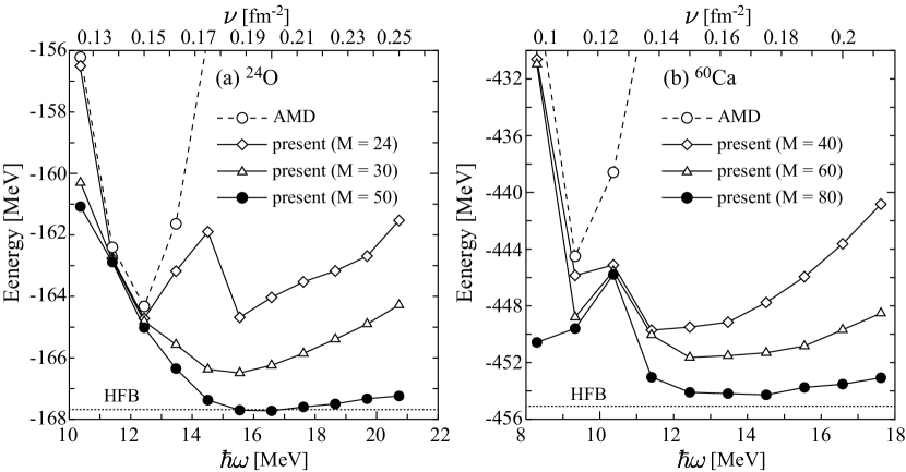
Figure 2: The calculated biding energies of ${}^{24}{\rm O}$ and ${}^{60}{\rm Ca}$ as functions of the the applied Gaussian size parameter, $\hbar\omega=2\hbar^{2}\nu/m$. The results are plotted for the different model space with $M=24$, 30 and 50 for ${}^{24}{\rm O}$, and $M=40$, 60 and 80 for ${}^{60}{\rm Ca}$. For comparison, the results of AMD and HFB are also shown. The results of HF(B) should also be dependent on the $\hbar\omega$ of the applied HO basis but no information was found in Ref. Hilaire2007 .

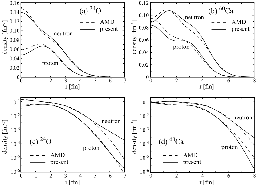
Figure 3: The calculated density distributions of protons and neutrons for ${}^{24}{\rm O}$ and ${}^{60}{\rm Ca}$ in comparison with those by the ordinary AMD. Upper and lower panels show them in the linear and logarithmic scales, respectively.

Table 1 and 2 show the optimized value of the width of LGs and the number of LGs required for the convergence. Compared to the AMD, the present model uses the LGs with narrower width to describe the fine structure of the single-particle wave functions. It is also shown that the number of LGs required for the convergence is much smaller than the 10 major shells of HO (220 basis). Figure 2 shows more detailed relationship between the energy, the width and number of LGs for the cases of ${}^{24}{\rm O}$ and ${}^{60}{\rm Ca}$. The energy calculated by AMD is strongly dependent on the magnitude of $\nu$, because it roughly determines the size and density of nucleus. On the other hand, the present model can flexibly describe various single-particle wave functions by superposing multiple LGs. Therefore, as the number of LGs increases, the dependence of the energy on $\nu$ becomes weaker, and the energy converges smoothly. In particular, the case of ${}^{60}{\rm Ca}$ is impressive. The ordinary AMD underestimates the binding energy about 10 MeV compared to HFB, while the present model gave the almost the same result with the HFB despite the lack of pairing correlations.

The improvement in the wave functions is well seen from the density distributions shown in Fig. 3. The upper panels of Fig. 3 show that the density distribution inside the nucleus has changed from that of AMD. This mainly owes to the improvement of the wave functions which have nodes inside the nucleus, such as the $2s_{1/2}$, $2p_{3/2}$ and $2p_{1/2}$. The lower panels of Fig. 3 show that the asymptotic forms outside the nucleus have also been improved. In AMD, both proton and neutron densities show Gaussian damping, and the damping rate is the same as they are described by a single Gaussian with a common value of the width parameter $\nu$. In contrast, the present model reasonably describes the exponential damping, and the damping rate is different for protons and neutrons reflecting the difference in their separation energies. In such a way, the present model greatly improves the wave functions inside and outside the nucleus.

Figure 4: The calculated density distributions of protons and neutrons for ${}^{100}{\rm Sn}$ in linear and ogarithmic scales. The number of superposed LGs is $M=100$, and the width of LGs is set to $\nu=0.1625$ fm^-2.

Finally, we demonstrate the applicability of the present model to the heavier mass systems. In the ordinary AMD, the structure calculation of such heavy nuclei was out of the scope due to the following reasons. When describing the shell structure of heavy nuclei with a limited number of LGs, the Gaussian centroids $\bm{z}_{p}$ are densely located near the center of mass increasing the overlap of LGs. Consequently, the matrix $d$ becomes ill-conditioned leading to the instability of the numerical calculations. This also makes it difficult to describe the almost constant and saturated density inside the heavy-mass nuclei. On the other hand, the present method superposes many LGs to describe the single-particle wave functions, so the overlap of LGs is not large and it is flexible enough to describe various density profiles.

As an example, for ${}^{100}{\rm Sn}$, the binding energy of 829.7 MeV was obtained by a superposition of a hundred LGs ($M=100$), which is 1.5 MeV deeper than the HFB with HO basis expansion Hilaire2007 . Note that the ordinary AMD cannot give the reasonable results for this nucleus. This again confirms the efficiency of the present model. The calculated density distributions of protons and neutrons are shown in Fig. 4. Although we cannot compare with AMD, the calculated density looks reasonable when compared with HF(B). The relatively constant density distribution inside the nucleus and the exponential damping outside the nucleus are plausibly described. The proton density distribution is slightly pushed outwards as this is a nucleus close to the proton drip line.

4 Conclusion

In this study, we have constructed a new framework using LGs and introduced its basic formulae. This framework describes the single-particle wave function as a superposition of LGs, where the weights of the superposition and the mean position and momentum of LGs are variational parameters. The energy variation consists of the equations determining the parameters for LGs and the amplitudes of the superposition. The former naturally extends the motion of Gaussian wave packets described in the microscopic cluster models, AMD, and FMD, while the latter is a Hartree-Fock equation which determines the single-particle wave function. Since the LGs themselves are variational functions, various nuclear structure and reaction problems can be efficiently described.

In the numerical calculations of oxygen and calcium isotopes using the Gogny D1S effective interaction, the new method improved upon the results of AMD, particularly in calcium isotopes. Moreover, for nuclei in which pairing energy is not significantly large, the new method yielded the results consistent to or better than HF(B) based on HO expansions. The proton and neutron density distributions revealed the improvement of the wave functions both inside and outside the nucleus with particularly accurate asymptotic behavior at large distances. The result for ${}^{100}{\rm Sn}$ also demonstrated the applicability of this method to the heavier mass nuclei. Based on these results, we expect that the new method will be useful for studying various nuclear structures and reaction dynamics.

Finally, we list some extensions of the framework to be done and reported in our future works:

• Use of deformed LGs Kimura2004 to describe deformed nuclei more efficiently.

• Introduction of pairing correlation.

• Parity, angular momentum, and particle number projections; and generator coordinate method for the beyond-mean field calculations.

• Extenstion to time-dependent calculations for applications to low-energy nuclear reactions and real-time evolution method

• Introduction of nucleon collision terms for the description of high-energy nuclear reactions and nuclear fragmentation.

Appendix A Supplementary formulas

Here, we summarize several formulae for the density matrix and the matrix element of two-body potential which are used for the energy variation.

A.1 The density matrix

As explained in the text, the density matrix is defined as $\rho^{\alpha}=\widetilde{c}^{\alpha}c^{\alpha\dagger}$ and $\bm{\rho}^{\alpha}=\widetilde{\bm{c}}^{\alpha}c^{\alpha\dagger}$. We remark that they satisfy the following identities,

$$N^{\alpha} ={\rm Tr}(d\rho^{\alpha}),$$ (26)

$$\rho^{\alpha} =\frac{1}{2}\set{\rho^{\alpha}d\rho^{\alpha}+\bm{\rho}^{\alpha}\cdot(d\bm{\rho}^{\alpha})},$$ (27)

$$\bm{\rho}^{\alpha} =\frac{1}{2}\set{\rho^{\alpha}d\bm{\rho}^{\alpha}+\bm{\rho}^{\alpha}d\rho^{\alpha}+i\bm{\rho}^{\alpha}\times(d\bm{\rho}^{\alpha})},$$ (28)

where $N^{\alpha}$ is the particle number with isospin $\alpha$. These identities reduce to the ordinary ones when $\ket{p}$ is orthonormal, i.e., $d_{pq}=\delta_{pq}$.

Straightforward calculation yields the derivative of the density matrix by $c_{tm}^{\alpha\dagger}$ as,

$$\partial^{\alpha}_{tm}\rho^{\alpha}_{rp} =\Bigl{\{}1-\frac{1}{2}d(\rho+\bm{\rho}\cdot\bm{\sigma})\Bigr{\}}_{tp}\widetilde{c}^{\alpha}_{rm},$$ (29)

$$\partial^{\alpha}_{tm}\bm{\rho}^{\alpha}_{rp} =\Bigl{\{}1-\frac{1}{2}d(\rho+\bm{\rho}\cdot\bm{\sigma})\Bigr{\}}_{tp}\widetilde{\bm{c}}^{\alpha}_{rm},$$ (30)

and the derivative by $\vec{z}^{*}_{t}$ as,

$$\vec{\partial}_{t}\rho_{rp}^{\alpha} =-\frac{1}{2}\left\{\rho^{\alpha}_{rt}(\vec{d}\rho^{\alpha})_{tp}+\bm{\rho}^{\alpha}_{rt}\cdot(\vec{d}\bm{\rho}^{\alpha})_{tp},\right\}$$ (31)

$$\vec{\partial}_{t}\bm{\rho}_{rp}^{\alpha} =-\frac{1}{2}\left\{\bm{\rho}^{\alpha}_{rt}(\vec{d}\rho^{\alpha})_{tp}+\rho^{\alpha}_{rt}(\vec{d}\bm{\rho}^{\alpha})_{tp}+i\bm{\rho}^{\alpha}_{rt}\times(\vec{d}\bm{\rho}^{\alpha})_{tp},\right\}$$ (32)

where $\vec{d}$ denotes the derivative of the overlap matrix of LGs that is defined as,

$$\vec{\partial}_{t}d_{pr} =-(\vec{z}_{t}^{*}-\vec{z}_{r})d_{tr}\delta_{tp}=:\vec{d}_{tr}\delta_{tp}.$$ (33)

In Eqs. (31) and (32), one must carefully distinguish two different vectors denoted by arrowed and bold fonts; e.g., the inner and outer products in the equations are the operations for the bold vectors. Using these formulae, it is easy to calculate the derivative of the Hamiltonian by the variational parameters as given in Eqs. (20) and (23).

A.2 The matrix element for the two-body potentials

The general form of the matrix element for spin and isospin dependent two-body potential is summarized as,

$$\braket{o}=\frac{1}{2}\sum_{pqrs}\sum_{\alpha\beta}(A^{\alpha\beta}_{pqrs}\rho_{rp}^{\alpha}\rho_{sq}^{\beta}+B^{\alpha\beta}_{pqrs}\bm{\rho}_{rp}^{\alpha}\cdot\bm{\rho}_{sq}^{\beta}+\bm{C}^{\alpha\beta}_{pqrs}\cdot\bm{\rho}_{rp}^{\alpha}\rho_{sq}^{\beta}+\bm{C}^{\alpha\beta}_{pqrs}\cdot\bm{\rho}_{sq}^{\beta}\rho_{rp}^{\alpha}),$$ (34)

where $A^{\alpha\beta}_{pqrs}$, $B^{\alpha\beta}_{pqrs}$ and $\bm{C}^{\alpha\beta}_{pqrs}$ are the functions of $\vec{z}^{*}_{p}$, $\vec{z}^{*}_{q}$, $\vec{z}_{r}$, and $\vec{z}_{s}$, and are independent of the spinors. In other words, one should arrange $A^{\alpha\beta}_{pqrs}$, $B^{\alpha\beta}_{pqrs}$ and $\bm{C}^{\alpha\beta}_{pqrs}$ so that the matrix element is expressed in the form of Eq. (34). Then, Eq. (34) can be simplified as,

$$\braket{o} =\frac{1}{2}\sum_{pr}\sum_{\alpha}(\Gamma^{\alpha}_{pr}\rho_{rp}^{\alpha}+\bm{\Gamma}^{\alpha}_{pr}\cdot\bm{\rho}_{rp}^{\alpha})=\frac{1}{2}\sum_{\alpha}\mathrm{Tr}(\Gamma^{\alpha}\rho^{\alpha}+\bm{\Gamma}^{\alpha}\cdot\bm{\rho}^{\alpha}),$$ (35)

$$\Gamma^{\alpha}_{pr} :=\sum_{sq}\sum_{\beta}(A^{\alpha\beta}_{pqrs}\rho_{sq}^{\beta}+\bm{C}^{\alpha\beta}_{pqrs}\cdot\bm{\rho}_{sq}^{\beta}),\quad\bm{\Gamma}^{\alpha}_{pr}:=\sum_{sq}\sum_{\beta}(B^{\alpha\beta}_{pqrs}\bm{\rho}_{sq}^{\beta}+\bm{C}^{\alpha\beta}_{pqrs}\rho_{sq}^{\beta}).$$ (36)

For example, the central two-body interaction of the Gogny force is given as the sum of the Gaussians,

$$v(\bm{r})=\sum_{n=1}^{2}(W_{n}+B_{n}P_{\sigma}-H_{n}P_{\tau}-M_{n}P_{\sigma}P_{\tau})e^{-r^{2}/\mu_{n}^{2}},$$ (37)

where $P_{\sigma}$ and $P_{\tau}$ are the spin and isospin exchange operators, respectively. In this case, $\bm{C}^{\alpha\beta}_{pqrs}=0$. $A^{\alpha\beta}_{pqrs}$ and $B^{\alpha\beta}_{pqrs}$ are given as,

$$A^{\alpha\beta}_{pqrs} :=\Set{(W_{n}+B_{n}/2)-\delta_{\alpha\beta}(H_{n}+M_{n}/2)}e_{pqrs}+(B_{n}/2-\delta_{\alpha\beta}M_{n}/2)e_{pqsr},$$ (38)

$$B^{\alpha\beta}_{pqrs} :=\Set{(M_{n}+H_{n}/2)-\delta_{\alpha\beta}(B_{n}+W_{n}/2)}e_{pqrs}+(H_{n}/2-\delta_{\alpha\beta}W_{n}/2)e_{pqsr},$$ (39)

$$e_{pqrs} :=(1-\lambda_{n})^{3/2}\exp\Set{-\frac{\lambda_{n}}{4}(\bm{z}_{p}^{*}-\bm{z}_{q}^{*}+\bm{z}_{r}-\bm{z}_{s})^{2}},\quad\lambda_{n}=(1+\nu\mu_{n}^{2})^{-1}.$$ (40)

Another example is the zero-range spin-orbit interaction which is defined as,

$$v(\bm{r})=iW(\bm{\sigma}_{1}+\bm{\sigma}_{2})\cdot\overleftarrow{\nabla}\times\delta(\bm{r})\overrightarrow{\nabla}.$$ (41)

For this, $A^{\alpha\beta}_{pqrs}=B^{\alpha\beta}_{pqrs}=0$, and

$$\bm{C}^{\alpha\beta}_{pqrs} =iW\nu\left(\frac{\nu}{\pi}\right)^{3/2}(1+\delta_{\alpha\beta})(\bm{z}^{*}_{p}-\bm{z}^{*}_{q})\times(\bm{z}_{r}-\bm{z}_{s})d_{pr}d_{qs}e_{pqrs},$$ (42)

$$e_{pqrs} :=\exp\Set{-\frac{1}{4}(\bm{z}_{p}^{*}-\bm{z}_{q}^{*}+\bm{z}_{r}-\bm{z}_{s})^{2}}.$$ (43)

Appendix B Stationary condition and Hartree-Fock equation

Here, we show that the stationary condition for $c^{\alpha}_{pi}$ given by Eq. (20) is equivalent to Eq. (22). To this end, it is convenient to extend the single-particle wave functions to include the unoccupied (particle) states.

$$\ket{i}=\sum_{p=1}^{M}\ket{p}c_{pi},\quad(i=1,...,2M,\quad p=1,...,M).$$ (44)

Note that the index $i$ runs up to $2M$ over the both occupied and unoccupied states. Hereafter, for simplicity, we omit the isospin index and let $N$ as the number of particles. We assume that the index $i$ is arranged so that $i\leq N$ correspond to the occupied (hole) states and $N<i\leq 2M$ correspond to the unoccupied (particle) states. We also assume that the occupied and unoccupied states are orthogonal, i.e.,

$$\braket{i}{j}=\sum_{pq}d_{pq}\braket{c_{pi}}{c_{qj}}=0\quad\text{for}\ i\leq N<j\leq 2M\ \text{or}\ j\leq N<i\leq 2M.$$ (45)

It is noted that this extension does not change the density matrix,

$$\rho=\sum_{ij=1}^{N}\braket{c_{pi}}{c_{qj}}{b}^{-1}_{ji},\quad\bm{\rho}=\sum_{ij=1}^{N}\braket{c_{pi}}{\bm{\sigma}}{c_{qj}}{b}^{-1}_{ji},$$ (46)

where the index $i$ and $j$ run up to $N$ for the occupied states. The stationary condition given by Eq. (20) also holds as it is for $i\leq N$.

Now we show that $(\rho+\bm{\rho}\cdot\bm{\sigma})d/2$ is the projection operator onto the occupied states, i.e.,

$$\frac{1}{2}(\rho+\bm{\rho}\cdot\bm{\sigma})d\widetilde{c}=\left\{\begin{array}[]{ll}\widetilde{c}&\text{for}\ i\leq N,\\ 0&\text{for}\ i>N.\end{array}\right.$$ (49)

(proof)

The left hand side of the equation is calculated as,

$$\frac{1}{2}\left[(\rho+\bm{\rho}\cdot\bm{\sigma})d\widetilde{c}\right]_{ql} =\frac{1}{2}\sum_{ijkpr}b^{-1}_{ji}b^{-1}_{kl}d_{pr}(\braket{c_{pi}}{c_{qj}}+\braket{c_{pi}}{\bm{\sigma}}{c_{qj}}\cdot\bm{\sigma})\ket{c_{rk}}$$

$$=\sum_{ijkpr}b^{-1}_{ji}b^{-1}_{kl}d_{pr}\braket{c_{pi}}{c_{rk}}\ket{c_{qj}},$$ (50)

where we have utilized the identity for the spinors,

$$\frac{1}{2}\left\{\ket{C}\braket{A}{B}+\bm{\sigma}\ket{C}\cdot\braket{A}{\bm{\sigma}}{B}\right\}=\ket{B}\braket{A}{C},$$ (51)

where $\ket{A}$, $\ket{B}$ and $\ket{C}$ denote independent spinors. In the last line of Eq. (50), $\sum_{pr}d_{pr}\braket{c_{pi}}{c_{rk}}$ is nothing but the ovelap of the single-particle states $\braket{i}{k}$ where $\ket{i}$ is an occupied state. Hence, it is equal to $b_{ik}$ if $\ket{k}$ is an occupied state, and it is zero if $\ket{k}$ is an unoccupied state. Thus, the identity given by Eq. (49) is proved.

Denoting this projection operator as $P$, the stationary condition given by Eq. (20) is rewritten as,

$$(1-P)d^{-1}(h+\bm{h}\cdot\bm{\sigma})\widetilde{c}=0.$$ (52)

Hence, the linear operator $d^{-1}(h+\bm{h}\cdot\bm{\sigma})$ and $P$ commutes. In other words, $d^{-1}(h+\bm{h}\cdot\bm{\sigma})$ does not mix the occupied and unoccupied states. From this and the positive definiteness of the matrix $d$, there exists a certain linear transformation between occupied states and that between the unoccupied states, which rearrange $\widetilde{c}$ to satisfy the set of $2M$ generalized eigenvalue equations,

$$(h+\bm{h}\cdot\bm{\sigma})\widetilde{c}=d\widetilde{c}\varepsilon,$$ (53)

where $\varepsilon=\mathrm{diag}(\varepsilon_{1},...,\varepsilon_{N},...,\varepsilon_{2M})$ are the single-particle energies of the occupied and unoccupied states. Thus, if Eq. (52) is satisfied, then Eq. (53) is also satisfied. Conversely, if Eq. (53) is satisfied, it is obvious that Eq. (52) is also satisfied. Hence, the equivalence of the stationary condition and the generalized eigenvalue equations is proved.

References

- (1) H. Feldmeier, T. Neff, R. Roth, and J. Schnack, Nuclear Physics A, 632, 61–95 (1998).
- (2) T. Neff and H. Feldmeier, Nuclear Physics A, 713, 311–371 (2003).
- (3) R. Roth, H. Hergert, P. Papakonstantinou, T. Neff, and H. Feldmeier, Physical Review C, 72, 034002 (2005).
- (4) Takayuki Myo, Hiroshi Toki, Kiyomi Ikeda, Hisashi Horiuchi, and Tadahiro Suhara, Progress of Theoretical and Experimental Physics, 2015, 073D02 (2015).
- (5) Takayuki Myo, Hiroshi Toki, Kiyomi Ikeda, Hisashi Horiuchi, and Tadahiro Suhara, Physical Review C, 96, 034309 (2017).
- (6) Tokuro Fukui, Progress of Theoretical and Experimental Physics, 2023 (2023).
- (7) D. Gogny, Nuclear Physics A, 237, 399–418 (1975).
- (8) M. Girod and B. Grammaticos, Physical Review C, 27, 2317–2339 (1983).
- (9) J.L. Egido, H.-J. Mang, and P. Ring, Nuclear Physics A, 334, 1–20 (1980).
- (10) J.L. Egido, J. Lessing, V. Martin, and L.M. Robledo, Nuclear Physics A, 594, 70–86 (1995).
- (11) J. Dobaczewski and P. Olbratowski, Computer Physics Communications, 158, 158–191 (2004).
- (12) M. V. Stoitsov, W. Nazarewicz, and S. Pittel, Physical Review C, 58, 2092–2098 (1998).
- (13) M.V. Stoitsov, J. Dobaczewski, W. Nazarewicz, and P. Ring, Computer Physics Communications, 167, 43–63 (2005).
- (14) H. Nakada, Nuclear Physics A, 764, 117–134 (2006).
- (15) H. Nakada, Nuclear Physics A, 808, 47–59 (2008).
- (16) Yukio Hashimoto, Physical Review C, 88, 034307 (2013).
- (17) D. M. Brink, Proc. Int. School of Physics Enrico Fermi, Course 36, Varenna,, (Academic Press, New York, 1965).
- (18) K. Wildermuth and Y. C. Tang, A Unified Theory of the Nucleus, (Vieweg+Teubner Verlag, 1977).
- (19) Sakae Saito, Progress of Theoretical Physics Supplement, 62, 11–89 (1977).
- (20) Hisashi Horiuchi, Progress of Theoretical Physics Supplement, 62, 90–190 (1977).
- (21) Akihiro Tohsaki-Suzuki, Progress of Theoretical Physics Supplement, 62, 191–235 (1977).
- (22) Masayasu Kamimura, Progress of Theoretical Physics Supplement, 62, 236–294 (1977).
- (23) M. Saraceno, P. Kramer, and F. Fernandez, Nuclear Physics A, 405, 88–108 (1983).
- (24) E. Caurier, B. Grammaticos, and T. Sami, Physics Letters B, 109, 150–154 (1982).
- (25) S. Drozdz, J. Okolowicz, and M. Ploszajczak, Physics Letters B, 109, 145–149 (1982).
- (26) Yoshiko Kanada-En’yo, Masaaki Kimura, and Hisashi Horiuchi, Comptes Rendus. Physique, 4, 497–520 (5 2003).
- (27) Yoshiko Kanada-En’yo, Masaaki Kimura, and Akira Ono, Progress of Theoretical and Experimental Physics, 2012, 1A202 (2012).
- (28) M. Kimura, T. Suhara, and Y. Kanada-En’yo, The European Physical Journal A, 52, 373 (2016).
- (29) H. Feldmeier, Nuclear Physics A, 515, 147–172 (1990).
- (30) H. Feldmeier, K. Bieler, and J. Schnack, Nuclear Physics A, 586, 493–532 (1995).
- (31) J.F. F. Berger, M. Girod, and D. Gogny, Computer Physics Communications, 63, 365–374 (1991).
- (32) S. Hilaire and M. Girod, The European Physical Journal A, 33, 237–241 (2007).
- (33) Akinobu Doté, Hisashi Horiuchi, and Yoshiko Kanada-En’yo, Physical Review C, 56, 1844–1854 (1997).
- (34) Y. Sugawa, M. Kimura, and H. Horiuchi, Progress of Theoretical Physics, 106, 1129–1152 (2001).
- (35) M. Kimura, Y. Sugawa, and H. Horiuchi, Progress of Theoretical Physics, 106, 1153–1177 (2001).
- (36) Masaaki Kimura, Physical Review C, 69, 044319 (2004).