Exploring the Connection Between the Normalized Power Prior and Bayesian Hierarchical Models

Abstract

The power prior is a popular class of informative priors for incorporating information from historical data. It involves raising the likelihood for the historical data to a power, which acts as a discounting parameter. When the discounting parameter is modeled as random, the normalized power prior is recommended. Bayesian hierarchical modeling is a widely used method for synthesizing information from different sources, including historical data. In this work, we examine the analytical relationship between the normalized power prior (NPP) and Bayesian hierarchical models (BHM) for i.i.d. normal data. We establish a direct relationship between the prior for the discounting parameter of the NPP and the prior for the variance parameter of the BHM. Such a relationship is first established for the case of a single historical dataset, and then extended to the case with multiple historical datasets with dataset-specific discounting parameters. For multiple historical datasets, we develop and establish theory for the BHM-matching NPP (BNPP) which establishes dependence between the dataset-specific discounting parameters leading to inferences that are identical to the BHM. Establishing this relationship not only justifies the NPP from the perspective of hierarchical modeling, but also provides insight on prior elicitation for the NPP. We present strategies on inducing priors on the discounting parameter based on hierarchical models, and investigate the borrowing properties of the BNPP.

Keywords— Bayesian analysis; Normalized power prior; Power prior; Bayesian hierarchical models.

1 Introduction

The power prior (Ibrahim and Chen, 2000) is a popular class of informative priors that allow the incorporation of historical data through a discounted likelihood. It is constructed by raising the historical data likelihood to a power $a_{0}$, where $0\leq a_{0}\leq 1$. The discounting parameter $a_{0}$ can be fixed or modeled as random. When it is modeled as random and estimated jointly with other parameters of interest (denoted by $\theta$), the normalized power prior (NPP) (Duan et al., 2006) is recommended as normalization is critical to enabling the prior to factor into a conditional distribution of $\theta$ given $a_{0}$ and a marginal distribution of $a_{0}$ (Neuenschwander et al., 2009).

Some theoretical properties of the NPP have been extensively studied. For example, Carvalho and Ibrahim (2021) show that the NPP is always proper when the initial prior is proper, and that, viewed as a function of the discounting parameter, the normalizing constant is a smooth and strictly convex function. Pawel et al. (2023a) derive the marginal posterior distribution of $a_{0}$ when a beta prior is used for $a_{0}$ for i.i.d. normal and binomial models, and show that, for these models, the marginal posterior for $a_{0}$ does not converge to a point mass at one when the sample size becomes arbitrarily large. Shen et al. (2024) extend these results by providing a formal analysis of the asymptotic behavior of the marginal posterior for $a_{0}$ for generalized linear models (GLMs). They show that the marginal posterior for the discounting parameter converges to a point mass at zero if there is any discrepancy between the historical and current data. They also show that the marginal posterior for $a_{0}$ does not converge to a point mass at one when the datasets are fully compatible, and yet, for an i.i.d. normal model and finite sample size, the marginal posterior for $a_{0}$ always has most mass around one when the datasets are fully compatible. Ye et al. (2022) prove that if the prior on $a_{0}$ is non-decreasing and if the difference between the sufficient statistics of the historical and current data is negligible from a practical standpoint, the marginal posterior mode of $a_{0}$ is close to one. Han et al. (2022) point out that the normalizing constant might be infinite with improper initial priors on $\theta$ for $a_{0}$ values close to zero, in which case the admissible set of the discounting parameter excludes values close to zero.

Several methods have been proposed which provide guidance on choosing the discounting parameter $a_{0}$ for the power prior, or the prior for $a_{0}$ for the NPP. Many quasi-Bayesian or empirical Bayes-type approaches have been developed to adaptively determine $a_{0}$ in the power prior based on the degree of congruence between the historical and current data (Gravestock et al. (2017); Gravestock and Held (2019); Liu (2018); Bennett et al. (2021); Pan et al. (2017); Psioda and Xue (2020)). Shen et al. (2024) provide a fully Bayesian approach for eliciting optimal beta priors on $a_{0}$ for the NPP based on two criteria. One criterion minimizes a weighted average of KL divergences between the marginal posterior for $a_{0}$ and user-specified target distributions based on hypothetical scenarios where there is no discrepancy and where there is a maximum tolerable discrepancy between two data sources. The other criterion minimizes a weighted average of mean squared errors based on the posterior mean of the parameter of interest when its hypothetical true value is equal to its estimate using the historical data, or when it differs from its estimate by a maximum tolerable amount. Banbeta et al. (2019) develop the dependent and robust dependent NPP which allow dependent discounting parameters for multiple historical datasets by placing a hierarchical prior on them.

Hierarchical modeling is one of the most common methods for synthesizing information from different sources (e.g., historical datasets) (Gelman et al., 2013). Chen and Ibrahim (2006) provide insights into eliciting a guide value for $a_{0}$ in the power prior using the Bayesian hierarchical models (BHM) by establishing an analytic relationship between $a_{0}$ and the variance parameter of the BHM. The analytic relationship was also established for generalized linear models and extended to the case with multiple historical datasets by Chen and Ibrahim (2006). Pawel et al. (2023b) generalize this connection to the NPP, and show that for i.i.d. normal data, the NPP with a beta prior on $a_{0}$ aligns based on the BHM with a generalized beta prior on the relative heterogeneity variance.

In this paper, we examine the analytical relationship between the NPP and the BHM for i.i.d. normal data. We establish a direct relationship between the prior for the discounting parameter of the NPP and the prior for the variance parameter of the BHM that leads to equivalent posterior inference for the two models. Such a relationship is first established for the case of a single historical dataset, and then extended to the case with multiple historical datasets with multiple discounting parameters. Establishing this relationship for multiple historical datasets is an entirely novel development. We develop a modified NPP, the BHM-matching normalized power prior (BNPP), that establishes dependence between the discounting parameters for the multiple historical datasets, resulting in inference for the parameter of interest that is identical to inference based on the BHM. Establishing this relationship not only justifies the NPP from the perspective of hierarchical modeling, but also provides insight on how one might elicit the prior for the discounting parameters through the lens of hierarchical modeling. If one starts with an appropriate prior on the variance parameter in a BHM, a prior on the discounting parameters in a BNPP is induced, providing a semi-automatic benchmark prior for discounting parameters in the NPP. Moreover, in the case of multiple historical datasets, the BNPP allows for dependent discounting of the historical datasets without the need to specify a prior for each discounting parameter, since each discounting parameter is shown to be a deterministic function of a single global discounting parameter. We present strategies on inducing priors on the discounting parameter based on the BHM, and extensively study the borrowing properties of the BNPP. We also demonstrate how our theoretical results can be applied more generally for non-normal data using asymptotics through a case study.

The rest of the paper proceeds as follows. In Section 2, we develop the formal analytical relationship between the NPP and the BHM when there is a single historical dataset for i.i.d. normal data. For multiple historical datasets, we define the BNPP and show the sufficient conditions under which it will produce equivalent posterior inference for the parameter of interest compared to the BHM. In Section 3, we visually examine the induced prior on $a_{0}$ based on choices of prior for the variance parameter in the BHM, and vice versa. We also explore the borrowing properties of the BNPP through extensive simulations and compare its performance to the NPP with independent priors on the discounting parameters. In Section 4, we apply the BNPP to real data from a pediatric lupus trial where the prior is formulated to borrow information from two adult trials. In Section 5, we close the paper with some discussion and thoughts on future research.

2 Analytical Connections between the Normalized Power Prior and Bayesian Hierarchical Models

We start by laying out the mathematical relationship between the NPP and the BHM, first for a single historical dataset and then for multiple historical datasets. For the multiple datasets case, the BHM is widely used.

2.1 Single Historical Dataset

We first consider i.i.d. normal data with a single historical dataset. Let $y=(y_{1},\dots,y_{n})$ denote the current data with sample size $n$. The current data model is

$$y_{i}\sim N(\theta,\sigma^{2}),$$

where $i=1,\dots,n$, and $\sigma^{2}$ is fixed and known. Let $y_{0}=(y_{01},\dots,y_{0n_{0}})$ denote the historical data with sample size $n_{0}$. The historical data model is

$$y_{0i}\sim N(\theta_{0},\sigma^{2}_{0}),$$

where $i=1,\dots,n_{0}$, and $\sigma^{2}_{0}$ is fixed and known.

The Bayesian hierarchical model (BHM) commonly uses priors of the form

$$\theta|\mu,v\sim N(\mu,v),\qquad\theta_{0}|\mu,v\sim N(\mu,v),$$

and hyperpriors

$$\mu\sim N(\alpha,\nu^{2}),\qquad v\sim IG(c,d),$$

where $\alpha$, $\nu$, $c$ and $d$ are fixed hyperparameters. Note that our theoretical development does not require the prior on $v$ to be the inverse Gamma distribution. For example, a half-normal prior as advocated by Gelman et al. (2013) could easily be used.

The joint posterior for $\theta$, $\theta_{0}$, $\mu$, and $v$ based on the BHM is given by

$$\pi(\theta,\theta_{0},\mu,v|y,y_{0})\propto\frac{1}{v}\exp\left\{-\frac{n(\bar{y}-\theta)^{2}}{2\sigma^{2}}-\frac{n_{0}(\bar{y}_{0}-\theta_{0})^{2}}{2\sigma_{0}^{2}}-\frac{(\theta-\mu)^{2}+(\theta_{0}-\mu)^{2}}{2v}-\frac{(\mu-\alpha)^{2}}{2\nu^{2}}\right\}\pi(v),$$

and the marginal posterior for the main effect $\theta$ is given by

$$\pi(\theta|y,y_{0})\propto\int\int\int \frac{1}{v}\exp\left\{-\frac{n(\bar{y}-\theta)^{2}}{2\sigma^{2}}-\frac{n_{0}(\bar{y}_{0}-\theta_{0})^{2}}{2\sigma_{0}^{2}}-\frac{(\theta-\mu)^{2}+(\theta_{0}-\mu)^{2}}{2v}-\frac{(\mu-\alpha)^{2}}{2\nu^{2}}\right\}\pi(v)d\theta_{0}d\mu dv.$$ (1)

The power prior (Ibrahim and Chen, 2000) is formulated as

$$\pi(\theta|D_{0},a_{0})\propto L(\theta|D_{0})^{a_{0}}\pi_{0}(\theta),$$

where $0\leq a_{0}\leq 1$ is the discounting parameter which discounts the historical data likelihood, and $\pi_{0}(\theta)$ is the initial prior for $\theta$. When $a_{0}$ is modeled as random, the normalized power prior (Duan et al., 2006) (NPP) is recommended. The NPP is formulated as

$$\pi(\theta,a_{0}|y_{0})\propto\frac{L(\theta|y_{0})^{a_{0}}\pi_{0}(\theta)}{c(a_{0})}\pi(a_{0}),$$

where $\pi(a_{0})$ is the prior for $a_{0}$ and $c(a_{0})=\int L(\theta|y_{0})^{a_{0}}\pi_{0}(\theta)d\theta$ is the normalizing constant which is a function of $a_{0}$. For the normal model specified above with the initial prior $\pi_{0}(\theta)\propto 1$, the NPP becomes

$$\pi(\theta,a_{0}|y_{0})\propto\frac{\left[\sigma_{0}^{-n_{0}}\exp\left\{-\frac{1}{2\sigma_{0}^{2}}\sum_{i=1}^{n_{0}}\left(y_{0i}-\theta\right)^{2}\right\}\right]^{a_{0}}}{c(a_{0})}\pi(a_{0}),$$

where $c(a_{0})=\int\left[\sigma_{0}^{-n_{0}}\exp\left\{-\frac{1}{2\sigma_{0}^{2}}\sum_{i=1}^{n_{0}}\left(y_{0i}-\theta\right)^{2}\right\}\right]^{a_{0}}d\theta$. Then the marginal posterior for $\theta$ based on the NPP is

$$\pi(\theta|y,y_{0})\propto\int\exp\left\{-\frac{1}{2\sigma^{2}}\sum_{i=1}^{n}\left(y_{i}-\theta\right)^{2}\right\}\frac{\left[\sigma_{0}^{-n_{0}}\exp\left\{-\frac{1}{2\sigma_{0}^{2}}\sum_{i=1}^{n_{0}}\left(y_{0i}-\theta\right)^{2}\right\}\right]^{a_{0}}}{c(a_{0})}\pi(a_{0})da_{0}.$$ (2)

When the parameter $v$ in the BHM and the parameter $a_{0}$ in the NPP are fixed, Theorem 2.2 in Chen and Ibrahim (2006) states that the posterior for $\theta$ based on the BHM and the posterior for $\theta$ based on the power prior match if and only if the prior expectation $E_{\text{BHM}}[\mu]=\alpha=0$, $\nu^{2}\rightarrow\infty$, and

$$a_{0}=\frac{1}{\frac{2vn_{0}}{\sigma_{0}^{2}}+1}.$$

This result connects the BHM and the power prior when $a_{0}$ is fixed. In this work, we extend this theorem to scenarios where $v$ is modeled as random for the BHM and $a_{0}$ is modeled as random for the NPP. Specifically, we show that there are in fact choices for (hyper)priors $\pi(v)$ in the BHM and $\pi(a_{0})$ in the NPP that lead to equivalent marginal posteriors for $\theta$.

Let $\pi_{\text{NPP}}(\theta|a_{0})$ denote the posterior for $\theta$ conditional on $a_{0}$ using the NPP and $\pi_{\text{BHM}}(\theta|v)$ denote the posterior for $\theta$ conditional on $v$ using the BHM. Our goal is to find a transformation from $a_{0}$ to $v$ such that the marginals of $\theta$ based on the two models are equivalent, i.e.,

$$\int\pi_{\text{NPP}}(\theta|a_{0})\pi(a_{0})da_{0}=\int\pi_{\text{BHM}}(\theta|v)\pi(v)dv.$$

That is, we want to find a function $a_{0}=f(v)$ such that

$$\int\pi_{\text{NPP}}(\theta|f(v))\pi(f(v))\left|\frac{df(v)}{dv}\right|dv=\int\pi_{\text{BHM}}(\theta|v)\pi(v)dv.$$

Theorem 2.1.

The marginal posterior for $\theta$ based on the BHM given in (1) and the marginal posterior for $\theta$ based on the NPP given in (2) are identical if and only if

$$a_{0}=f(v)=\frac{1}{\frac{2vn_{0}}{\sigma_{0}^{2}}+1}$$

and if

$$\left(\frac{2vn_{0}}{\sigma_{0}^{2}}+1\right)^{-2}\pi(f(v))=\pi(v).$$

Proof.

See Appendix A.1. ∎

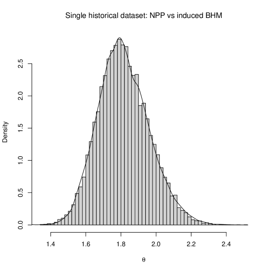
Figure 6: Single historical dataset: in this example, $n=n_{0}=20$, $\bar{y}=2$, $\bar{y}_{0}=1.5$, $\sigma^{2}=0.5$ and $\sigma^{2}_{0}=0.3$. We ran four independent chains of 10,000 iterations with 5,000 burn-ins. The histogram represents the posterior of $\theta$ using a normalized power prior with a beta($2$, $2$) prior on $a_{0}$. The density curve represents the posterior of $\theta$ using the BHM where the prior on $v$ is induced using Theorem 2.1. We observe that the two posteriors are equivalent.

Theorem 2.1 gives us a direct relationship between the prior for $a_{0}$ in the NPP and the prior for the variance parameter of the BHM. Note that the transformation from $a_{0}$ to $v$ used here is the same as in Theorem 2.2 in Chen and Ibrahim (2006). In the Appendix, we provide Figure 6 that illustrates empirically that the formulas in Theorem 2.1 lead to equivalent posteriors for $\theta$ based on the BHM and the NPP. Note that the result of Theorem 2.1 is similar to equation (20) in Pawel et al. (2023b); our result was derived independently.

2.2 BHM-matching Normalized Power Prior (BNPP) for Multiple Historical Datasets

We now consider i.i.d. normal data with historical datasets $k=1,\dots,K$. Let $y=(y_{1},\dots,y_{n})$ denote the current data with sample size $n$. The model for the current data is

$$y_{i}\sim N(\theta,\sigma^{2}),$$

where $i=1,\dots,n$, and $\sigma^{2}$ is fixed and known. Let $y_{0}=(y_{01},\dots,y_{0K})$ denote the $K$ historical datasets each with sample size $n_{01},\dots,n_{0K}$, where $y_{0k}=(y_{0k1},\dots,y_{0kn_{0k}})$ for $k=1,\dots,K$. The historical data model is

$$y_{0ki}\sim N(\theta_{0k},\sigma^{2}_{0k}),$$

where $i=1,\dots,n_{0k}$, and $\sigma^{2}_{0k}$’s are fixed and known. Let $\theta_{0}=(\theta_{01},\dots,\theta_{0K})$.

The Bayesian hierarchical model (BHM) commonly uses priors that take the form

$$\theta|\mu,v\sim N(\mu,v),\qquad\theta_{0k}|\mu,v\sim N(\mu,v),$$

and

$$\mu\propto 1,\qquad v\sim IG(c,d),$$

where $c$ and $d$ are fixed hyperparameters. We use $\pi(\mu)\propto 1$ here because the result in Theorem 2.1 can be obtained alternatively by using a uniform improper prior for $\mu$ at the outset (see Corollary 2.2. in Chen and Ibrahim (2006)). Then the joint posterior for $\theta$, $\theta_{0}$, $\mu$, and $v$ based on the BHM is given by

$$\pi(\theta,\theta_{0},\mu,v|y,y_{0})\propto \hskip 5.69046pt\pi(v)v^{-(K+1)/2}$$

$$\exp\left\{\frac{-n(\bar{y}-\theta)^{2}}{2\sigma^{2}}-\frac{1}{2}\sum_{k=1}^{K}\frac{n_{0k}(\bar{y}_{0k}-\theta_{0k})^{2}}{\sigma^{2}_{0k}}-\frac{(\theta-\mu)^{2}}{2v}-\frac{1}{2v}\sum_{k=1}^{K}(\theta_{0k}-\mu)^{2}\right\},$$

and the marginal posterior for $\theta$ is given by

$$\pi(\theta|y,y_{0})\propto\int\int\int\pi(v)v^{-(K+1)/2}\exp\left\{\frac{-n(\bar{y}-\theta)^{2}}{2\sigma^{2}}-\frac{1}{2}\sum_{k=1}^{K}\frac{n_{0k}(\bar{y}_{0k}-\theta_{0k})^{2}}{\sigma^{2}_{0k}}-\frac{(\theta-\mu)^{2}}{2v}-\frac{1}{2v}\sum_{k=1}^{K}(\theta_{0k}-\mu)^{2}\right\}d\theta_{0}d\mu dv.$$ (3)

When there are multiple historical datasets, we assume $a_{0}=(a_{01},\dots,a_{0K})$ are the discounting parameters with $a_{0k}$ corresponding to historical dataset $k$. When the $a_{0k}$’s are given independent priors, the normalized power prior (henceforth abbreviated iNPP) for $\theta$ and $a_{0}$ is given by

$$\pi_{iNPP}(\theta,a_{0}|y,y_{0})\propto\exp\left\{-\frac{1}{2\sigma^{2}}\sum_{i=1}^{n}(y_{i}-\theta)^{2}\right\}\frac{\prod_{k=1}^{K}\left[\sigma_{0k}^{-n_{0k}}\exp\left\{-\frac{1}{2\sigma_{0k}^{2}}\sum_{i=1}^{n_{0k}}\left(y_{0ki}-\theta\right)^{2}\right\}\right]^{a_{0k}}}{c(a_{0})}\prod_{k=1}^{K}\pi(a_{0k}),$$

with

$$c(a_{0})=\int\prod_{k=1}^{K}\left[\sigma_{0k}^{-n_{0k}}\exp\left\{-\frac{1}{2\sigma_{0k}^{2}}\sum_{i=1}^{n_{0k}}\left(y_{0ki}-\theta\right)^{2}\right\}\right]^{a_{0k}}d\theta.$$

In order to establish a correspondence between the NPP and the BHM for multiple historical datasets, we must assume some relationship between the discounting parameters in the NPP. We define the BHM-matching NPP (BNPP) as follows:

$$\pi_{BNPP}(\theta,a_{0}|y,y_{0})\propto\exp\left\{-\frac{1}{2\sigma^{2}}\sum_{i=1}^{n}(y_{i}-\theta)^{2}\right\}\frac{\prod_{k=1}^{K}\left[\sigma_{0k}^{-n_{0k}}\exp\left\{-\frac{1}{2\sigma_{0k}^{2}}\sum_{i=1}^{n_{0k}}\left(y_{0ki}-\theta\right)^{2}\right\}\right]^{h_{k}(a_{0})}}{c(a_{0})}\pi(a_{0}),$$

where $0<h_{k}(a_{0})<1$ is a transformation of $a_{0}$ which discounts the $k^{th}$ historical dataset, and

$$c(a_{0})=\int\prod_{k=1}^{K}\left[\sigma_{0k}^{-n_{0k}}\exp\left\{-\frac{1}{2\sigma_{0k}^{2}}\sum_{i=1}^{n_{0k}}\left(y_{0ki}-\theta\right)^{2}\right\}\right]^{h_{k}(a_{0})}d\theta.$$

Then the marginal posterior for $\theta$ with the BNPP is

$$\pi_{BNPP}(\theta|y,y_{0})\propto\int\exp\left\{-\frac{1}{2\sigma^{2}}\sum_{i=1}^{n}(y_{i}-\theta)^{2}\right\}\frac{\prod_{k=1}^{K}\left[\sigma_{0k}^{-n_{0k}}\exp\left\{-\frac{1}{2\sigma_{0k}^{2}}\sum_{i=1}^{n_{0k}}\left(y_{0ki}-\theta\right)^{2}\right\}\right]^{h_{k}(a_{0})}}{c(a_{0})}\pi(a_{0})da_{0}.$$ (4)

Our goal is to characterize $h_{k}(a_{0})$ and the transformation $a_{0}=f(v)$ such that

$$\int\pi_{\text{BNPP}}(\theta|f(v))\pi(f(v))\left|\frac{df(v)}{dv}\right|dv=\int\pi_{\text{BHM}}(\theta|v)\pi(v)dv.$$

Theorem 2.2.

The marginal posterior for $\theta$ based on the BHM given in (3) and the marginal posterior for $\theta$ based on the BNPP given in (4) are identical if

$$a_{0}=f(v)=\left[1+\sum_{k=1}^{K}\frac{\frac{n_{0k}}{\sigma^{2}_{0k}}}{\frac{n_{0k}}{\sigma^{2}_{0k}}+\frac{1}{v}}\right]^{-1},$$

$$h_{k}(a_{0})=\left(1+\frac{n_{0k}v}{\sigma^{2}_{0k}}\right)^{-1}a_{0},$$

and

$$Q(f(v))\cdot\left|\frac{df(v)}{dv}\right|\pi(f(v))=R(v)\cdot\pi(v),$$

where

$$Q(f(v))=\exp\left\{-\frac{f(v)}{2C}\left(\frac{1}{v}\sum_{k=1}^{K}N_{k}Y_{k}\right)^{2}\right\}\left[f(v)C\right]^{\frac{1}{2}}$$

and

$$R(v)=v^{-(K+1)/2}\prod_{k=1}^{K}N_{k}^{\frac{1}{2}}A^{-\frac{1}{2}}\exp\left\{\frac{\left(\sum_{k=1}^{K}Y_{k}N_{k}\right)^{2}}{2v^{2}A}\right\}\exp\left\{\frac{1}{2}\sum_{k=1}^{K}Y_{k}^{2}N_{k}\right\},$$

with $N_{k}=\left(\frac{n_{0k}}{\sigma^{2}_{0k}}+\frac{1}{v}\right)^{-1}$, $C=\sum_{k=1}^{K}\frac{n_{0k}N_{k}}{v\sigma^{2}_{0k}}$, $Y_{k}=\frac{n_{0k}\bar{y}_{0k}}{\sigma^{2}_{0k}}$ and $A=\frac{1+K}{v}-\frac{\sum_{k=1}^{K}N_{k}}{v^{2}}$. The Jacobian $\left|\frac{df(v)}{dv}\right|$ is given in the proof.

Proof.

See Appendix A.2. ∎

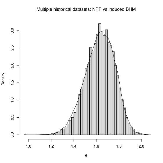
Figure 7: Multiple historical datasets: in this example, there are three historical datasets, and $n=30$, $n_{0}=(20,30,50)$, $\sigma^{2}=0.5$, $\sigma^{2}_{0}=(0.5,1,1.5)$, $\bar{y}_{0}=(1,2,3)$, and $\bar{y}=1.5$. We ran four independent chains of 8,000 iterations with 4,000 burn-ins. The histogram represents the posterior of $\theta$ using a normalized power prior with beta($2$, $2$) prior on $a_{0}$ and $h_{k}(a_{0})$ chosen according to Theorem 2.2. The density curve represents the posterior of $\theta$ using the BHM where the prior on $v$ is induced using Theorem 2.2. We observe that the two posteriors are equivalent.

For the BNPP, $h_{k}(a_{0})$ is a function of the global discounting parameter $a_{0}$ and the variance and sample size of the $k^{th}$ historical dataset. Theorem 2.2 gives a direct relationship between the prior for $a_{0}$ in the BNPP and the prior for the variance parameter of the BHM. Figure 7 in the Appendix illustrates empirically that the formulas in Theorem 2.2 lead to equivalent posteriors for $\theta$ based on the BHM and BNPP.

3 Simulations

3.1 Single historical dataset

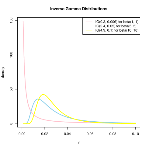
Figure 8: We choose three beta distributions with mean equal to $0.5$ as the prior for $a_{0}$ in the normalized power prior, and find the best approximating inverse gamma distribution prior for $v$ in a BHM. We observe that as we borrow more historical information, i.e. as the variance of the beta distribution decreases, the variance of the prior on $v$ also decreases, i.e. more historical information is borrowed.

In this section, we explore the connection between the prior on $a_{0}$ for the NPP and the prior on $v$ for the BHM when there is a single historical dataset. Applying the formulas provided in Theorem 2.1, we plot the induced priors on $v$ based on example choices of prior on $a_{0}$ (e.g., the uniform prior) in the NPP in Figure 1. In Figure 8 in the Appendix, we provide similar plots for three beta priors for $a_{0}$ each having mean equal to $0.5$ in the NPP, and derive the corresponding inverse gamma distribution prior for $v$ in a BHM. Conversely, we also plot the priors induced on $a_{0}$ based on example choices of prior on $v$ from the inverse gamma family in the BHM in Figure 2.

In Figure 1, beta(1,1), beta(0.5,0.5), beta(2,10) and beta(10,2) distributions are considered for the prior for $a_{0}$ in the NPP. The figure also presents the inverse gamma prior that matches most closely to the prior for $v$ induced by the prior on $a_{0}$ based on the formula in Theorem 2.1. Specifically, we solve for the inverse gamma distribution which minimizes the Kullback–Leibler (KL) divergence from the induced prior on $v$. We observe that as the prior on $a_{0}$ encourages more borrowing of historical information, i.e. as the expectation of the beta distribution increases, the expectation of the prior on $v$ decreases, i.e., the prior on $v$ correspondingly encourages more borrowing. For example, as illustrated by the two plots in the second row, in the left plot, a beta(2,10) prior on $a_{0}$ is concentrated near zero, indicating that borrowing is discouraged, and the corresponding prior on $v$ has relatively large variance. In the right plot, a beta(10,2) prior on $a_{0}$ is concentrated near one, indicating that borrowing is encouraged, and the corresponding prior on $v$ is much more concentrated near zero, also indicating that borrowing is encouraged.

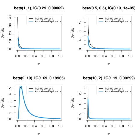
Figure 1: We choose four beta distributions as the prior for $a_{0}$ in the NPP, and find the best approximating inverse gamma distribution prior for $v$ in a BHM. The black line represents the induced prior on $v$ using Theorem 2.1, and the blue line represents the inverse gamma distribution that best approximates the induced prior.

In Figure 2, we choose IG(3,10), IG(3,1), IG(1,0.1), IG(1,0.01) as the prior for $v$ in the BHM, and find the beta prior that most closely matches the induced prior on $a_{0}$ based on the formula in Theorem 2.1. Specifically, we draw samples of $v$ from the inverse gamma distributions and transform them to samples of $a_{0}$. We then use beta regression to solve for the closest beta distribution that fits the $a_{0}$ samples. In the first row, in the left plot, the IG(3,10) distribution has mean equal to 5 and variance equal to 25, and the corresponding beta distribution is highly concentrated near zero, indicating that borrowing is discouraged. By comparison, in the right plot, the IG(3,1) distribution has mean equal to 0.5 and variance equal to 0.25, supporting comparatively more borrowing, and the corresponding prior on $a_{0}$ is much less concentrated near zero.

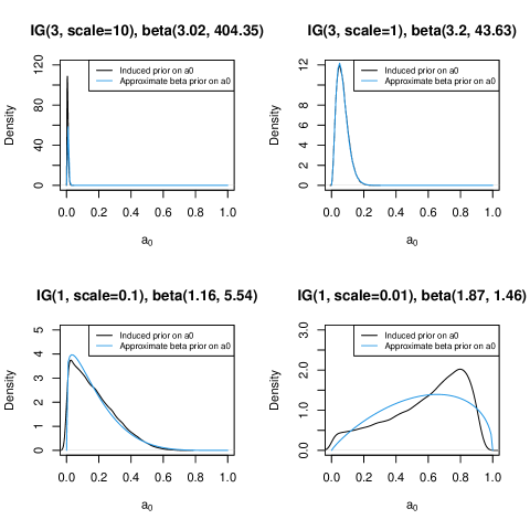
Figure 2: We choose four inverse gamma distributions as the prior for $v$ in the BHM, and find the best approximating beta prior for $a_{0}$ in a NPP. We draw samples of $v$ from the inverse gamma distributions and transform them to samples of $a_{0}$ using the formula in Theorem 2.1. We use beta regression to solve for the beta distribution that best fits the $a_{0}$ samples. The black line represents the induced prior on $a_{0}$ using Theorem 2.1, and the blue line represents the beta distribution that best approximates the induced prior.

3.2 Multiple historical datasets

When there are multiple historical datasets from which to borrow information, we explore the behavior of the BNPP and compare it to the NPP with independent $a_{0}$’s (iNPP) for various generated data scenarios. In the following set of simulations, we assume the current data $y_{1},\dots,y_{n}$ are i.i.d. observations from a $N(\theta,\sigma^{2})$ distribution. We also assume there are two historical datasets, where $y_{0k1},\dots,y_{0kn_{0k}}$ are i.i.d. observations from a $N(\theta,\sigma^{2}_{0k})$ where $k=1,2$. Let $\bar{y}$ denote the mean of the current data, and $\bar{y}_{01}$ and $\bar{y}_{02}$ denote the mean of the first and second historical datasets, respectively. Let $a_{01}$ and $a_{02}$ denote the discounting parameters for the first and second historical datasets, respectively. We assume independent uniform priors for $a_{01}$ and $a_{02}$ for the iNPP. For the BNPP, $a_{01}=h_{1}(a_{0})$ and $a_{02}=h_{2}(a_{0})$, and the prior on $v$ is chosen so that the conditions in Theorem 2.2 are satisfied where the prior on $a_{0}$ is the uniform distribution. We choose $\sigma^{2}=\sigma^{2}_{01}=\sigma^{2}_{02}=1$, $\bar{y}=0$ and $n=30$. We vary the means and the sample sizes of the historical datasets to investigate the performance of the BNPP and iNPP under various degrees of compatibility between the current and historical datasets. Specifically, through the marginal posteriors for $a_{01}$, $a_{02}$ and $\theta$, we examine how much historical information is borrowed and its impact on the inference of the main effect $\theta$ using the BNPP and iNPP. The BNPP is implemented with RStan (Stan Development Team, 2024) and the iNPP is implemented using the R package BayesPPD (Shen et al., 2023a, b).

For the BNPP, since $a_{0k}$ is a function of only $\sigma^{2}_{0k}/n_{0k}$ and $v$, and we fix $\sigma^{2}_{01}=\sigma^{2}_{02}=1$ for these simulations, the posterior densities of $a_{01}$ and $a_{02}$ will only differ if $n_{01}$ and $n_{02}$ differ. In addition, since $a_{0k}$ monotonically increases with $\sigma^{2}_{0k}/n_{0k}$, given equal variances for the historical datasets, the posterior density of $a_{0k}$ is more concentrated near zero, i.e., the historical dataset is discounted more, for larger sample sizes. For the BHM, it is well known that groups that have smaller sample size experience greater shrinkage toward the grand mean (Berry et al., 2013), so for the NPP, the smaller historical dataset has to be weighted comparatively more for the NPP to match the BHM.

In Figures 3 and 4, the first column includes density plots of the current data (black line) and two historical datasets (yellow and blue lines). The second column includes plots of the posterior densities of $a_{01}$ and $a_{02}$ using the BNPP (yellow and blue solid lines) and the iNPP (yellow and blue dashed lines). The third column includes plots of the posterior densities of $\theta$ using four different priors, the BNPP (purple), the iNPP (grey), the power prior with $a_{0}=0$ (black) and the power prior with $a_{0}=1$ (pink). In the top row of Figure 3, the current and historical datasets have the same mean, and the posteriors for $a_{01}$ and $a_{02}$ are similar using the BNPP and iNPP, and they both have modes at one. We also observe that the iNPP borrows more from the larger dataset compared to the BNPP. The posteriors for $\theta$ using the two priors are both centered at zero, yielding smaller variance than the analysis with the power prior that takes $a_{0}=0$. In the bottom row, the two historical datasets have the same mean but that mean differs substantially from the current data mean. In this case, the posteriors for $a_{01}$ and $a_{02}$ using the BNPP are concentrated near zero, while the iNPP results in significantly less discounting. As expected, the posterior for $\theta$ using the BNPP (purple line) is much closer to that using only the current data (black line).

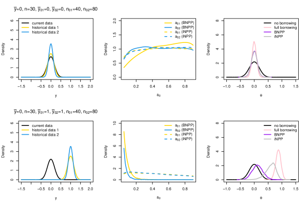
Figure 3: Marginal posteriors for $a_{01}$, $a_{02}$ and $\theta$ using the BNPP and the iNPP for simulated i.i.d. normal data. In the top row, the three datasets are fully compatible. In the bottom row, the two historical datasets are compatible but they are both incompatible with the current dataset. The first column includes plots of the densities of the current data (black line) and two historical datasets (yellow and blue lines). The second column includes plots of the posterior densities of $a_{01}$ and $a_{02}$ using the BNPP (yellow and blue solid lines) and the iNPP (yellow and blue dashed lines). The third column includes plots of the posterior densities of $\theta$ using four different priors, the BNPP (purple), the iNPP (grey), the power prior with $a_{0}=0$ (black) and the power prior with $a_{0}=1$ (pink).

In Figure 4, we assume one of the historical datasets is compatible with the current data while the other is not. In the top row, the historical dataset with the greater sample size is incompatible with the current data, while in the bottom row, the historical dataset with the greater sample size is compatible with the current data. We observe that, for both cases, the iNPP leads to more borrowing from the compatible historical dataset and less borrowing from the incompatible one in comparison to the BNPP. The BNPP discounts in accordance with the overall amount of conflict between the three datasets, and discounts more for more incompatible datasets (e.g., the top row). In the top row, the posterior for $\theta$ using the BNPP is closer to that using only the current data compared to the iNPP, due to less borrowing. In the bottom row, we can see that the posterior mean of $\theta$ is larger for the iNPP than the full borrowing case (power prior with $a_{0}=1$); this is because the first historical dataset has the same mean as the current dataset and full borrowing will lead to a mean closer to the current data mean. Moreover, the posterior for $\theta$ with iNPP is closer to that using only current data compared to the BNPP; this is because the iNPP leads to more borrowing from the compatible historical dataset and less from the incompatible historical dataset when compared to the BNPP.

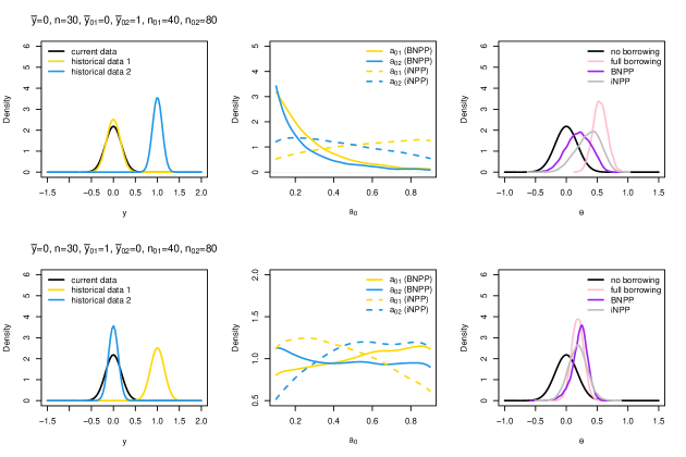
Figure 4: Marginal posteriors for $a_{01}$, $a_{02}$ and $\theta$ using the BNPP and the iNPP for simulated i.i.d. normal data. In these scenarios, one of the historical datasets is compatible with the current data while the other is not. The first column includes plots of the densities of the current data (black line) and two historical datasets (yellow and blue lines). The second column includes plots of the posterior densities of $a_{01}$ and $a_{02}$ using the BNPP (yellow and blue solid lines) and the iNPP (yellow and blue dashed lines). The third column includes plots of the posterior densities of $\theta$ using four different priors, the BNPP (purple), the iNPP (grey), the power prior with $a_{0}=0$ (black) and the power prior with $a_{0}=1$ (pink).

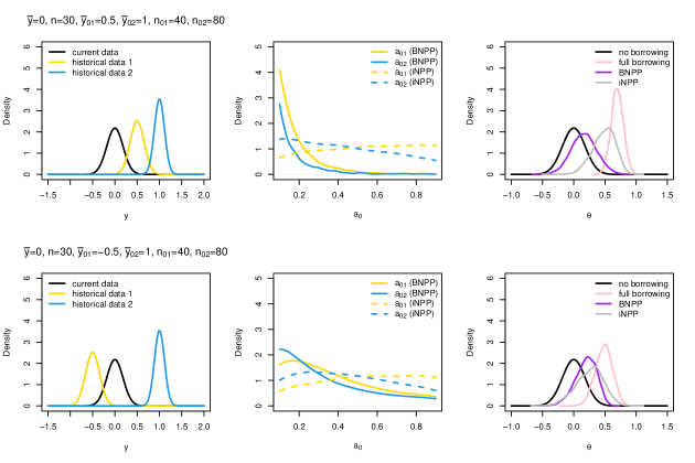
Figure 9: Marginal posteriors of $a_{01}$, $a_{02}$ and $\theta$ using the BNPP and the independent NPP for simulated i.i.d. normal data. In these scenarios, one of the historical datasets is incompatible with the current data while the other is partially compatible. The first column includes plots of the densities of the current data (black line) and two historical datasets (yellow and blue lines). The second column includes plots of the posterior densities of $a_{01}$ and $a_{02}$ using the BNPP (yellow and blue solid lines) and the iNPP (yellow and blue dashed lines). The third column includes plots of the posterior densities of $\theta$ using four different priors, the BNPP (purple), the iNPP (grey), the power prior with $a_{0}=0$ (black) and the power prior with $a_{0}=1$ (pink).

In summary, the BNPP and iNPP behave similarly when the historical and current datasets are compatible. The BNPP is more sensitive to conflicts in the data than the iNPP, and it tends to borrow more from the smaller dataset. When one of the historical datasets is compatible with the current data while the other is not, the iNPP borrows more from the compatible historical dataset compared to the BNPP which effectively bases discounting on the overall heterogeneity across all datasets. We include additional simulations when the historical datasets are partially compatible with the current dataset in Figure 9 in the Appendix.

4 Analysis of Pediatric Lupus Trial

We now demonstrate the use of the BNPP through an important application in a pediatric lupus clinical trial, where historical data from an adult phase 3 program is publicly available. Borrowing information from adult trials, so-called, partial extrapolation, is an increasingly common strategy in pediatric drug development due to the challenges in enrolling pediatric patients in clinical trials and the ability of regulators to require trials in these populations (U.S. Food and Drug Administration, 2016). The enrollment of patients in pediatric trials is often challenging due to the limited number of available patients, parental safety concerns, and technical limitations (Greenberg et al., 2018). Utilizing Bayesian methods for extrapolating adult data in pediatric trials through informative priors is a natural approach, as illustrated in the FDA guidance on complex innovative designs (U.S. Food and Drug Administration, 2019).

Belimumab (Benlysta) is a biologic for the treatment of adults with active, autoantibody-positive systemic lupus erythematosus (SLE). As a part of the pediatric investigation plan, the PLUTO clinical trial (Brunner et al., 2020) was conducted to evaluate the effect of belimumab on children aged 5 to 17 with active, seropositive SLE who receive standard therapy. Previous phase 3 trials, BLISS-52 and BLISS-76 (Furie et al., 2011; Navarra et al., 2011), established the efficacy of belimumab alongside standard therapy for adults. The FDA review of the PLUTO trial submission utilized data from these adult trials to inform the approval decision. All three trials shared the same composite primary outcome, the SLE Responder Index (SRI-4).

We perform a Bayesian analysis of the PLUTO study data ($n=92$), incorporating information from adult studies BLISS-52 ($n_{01}=548$) and BLISS-76 ($n_{02}=577$) using the BNPP and the iNPP. Since Theorem 2.2 requires i.i.d. normal data but our trial outcomes are binary, the theorem does not directly apply without approximation. Here, we assume the log odds ratio of receiving treatment is approximately normally distributed. Let $n_{t}$ and $n_{c}$ denote the number of patients in the treatment and control group in the PLUTO study, respectively. Let $p_{t}$ and $p_{c}$ denote the probability of response to treatment in the treatment and control group, respectively. The parameter of interest is the log odds ratio, denoted by $\theta$. It can be estimated by

$$\hat{\theta}=\log\left(\frac{\hat{p}_{t}}{1-\hat{p}_{t}}\right)-\log\left(\frac{\hat{p}_{c}}{1-\hat{p}_{c}}\right),$$

with asymptotic variance given by

$$Var(\hat{\theta})=\frac{1}{n_{t}p_{t}}+\frac{1}{n_{t}(1-p_{t})}+\frac{1}{n_{c}p_{c}}+\frac{1}{n_{c}(1-p_{c})}.$$

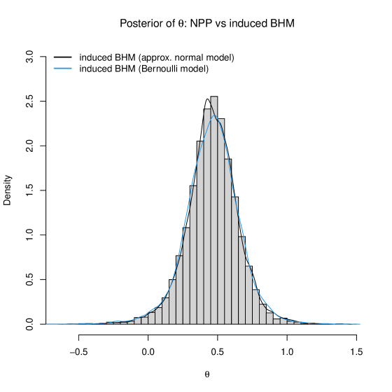
Figure 10: Pediatric lupus trial: the histogram represents the posterior of $\theta$ using a BNPP with a uniform prior on $a_{0}$ and $h_{k}(a_{0})$ chosen according to Theorem 2.2. The black density curve represents the posterior of $\theta$ using the BHM where the prior on $v$ is induced using Theorem 2.2. We observe that the two posteriors are equivalent. They are also equivalent to the posterior of $\theta$ using a Bernoulli model (blue curve) for the induced BHM. We ran four independent chains of 10,000 iterations with 5,000 burn-ins.

The approximate mean and variance of $\theta$ for the two adult studies can be computed analogously. For each current and historical dataset, we construct an approximation normal likelihood with sample size one, mean $\hat{\theta}$ and known variance Var($\hat{\theta}$), so that Theorem 2.2 can be applied. Let $a_{01}$ and $a_{02}$ denote the discounting parameters for BLISS-52 and BLISS-76, respectively. We assume independent uniform priors for $a_{01}$ and $a_{02}$ for the iNPP. For the BNPP, $a_{01}=h_{1}(a_{0})$ and $a_{02}=h_{2}(a_{0})$, and we use the induced prior on $v$ by Theorem 2.2 where $\pi(a_{0})$ is the uniform distribution. In the Appendix, we provide Figure 10 that corroborates empirically that the resulting posteriors for $\theta$ based on the BHM and the BNPP using the approximate normal model are equivalent, and they are also equivalent to the posterior for $\theta$ using a Bernoulli model for the induced BHM.

Figure 5 shows the approximate normal likelihoods of the log odds ratio for the three datasets and the marginal posteriors for $a_{01}$, $a_{02}$ and $\theta$ for the BNPP and iNPP. We can see that the estimates of the log odds ratios are quite similar for the adult studies and the pediatric study, although the variance is much smaller for the adult studies due to their larger sample sizes. The posteriors for $a_{01}$ and $a_{02}$ using BNPP and iNPP are similar, and they both have modes at one. The BNPP leads to more borrowing from the smaller dataset, while the iNPP leads to more borrowing from the larger dataset. The posteriors for $\theta$ using the two models are almost identical. The posterior means using the BNPP and iNPP are similar to that of the no borrowing model, but the posterior variances are much smaller. The posterior mean, standard deviation, and 95% credible interval for $\theta$, $a_{01}$ and $a_{02}$ for the BNPP and iNPP are displayed in Table 1. The posterior means of $\theta$ are similar for the two models. The posterior means of $a_{01}$ and $a_{02}$ using the BNPP are slightly higher than those of the iNPP, indicating more information borrowed.

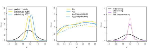
Figure 5: Marginal posteriors for $a_{01}$, $a_{02}$ and $\theta$ using the BNPP and the iNPP for the pediatric lupus study. The first column includes plots of the approximate normal densities of the log odds ratio of the PLUTO study (black line) and the two adult studies (yellow and blue lines). The second column includes plots of the posterior densities of $a_{01}$ and $a_{02}$ using the BNPP (yellow and blue solid lines) and the iNPP (yellow and blue dashed lines). The third column includes plots of the posterior densities of $\theta$ using four different priors, the BNPP (purple), the iNPP (grey), the power prior with $a_{0}=0$ (black) and the power prior with $a_{0}=1$ (pink).

Table 1: Pediatric lupus trial: posterior mean, standard deviation, and 95% credible interval for $\theta$, $a_{01}$ and $a_{02}$

Parameter	Mean	SD	95% Credible Interval
BHM-matching NPP
$\theta$	0.46	0.18	(0.08, 0.81)
$a_{01}$	0.53	0.28	(0.05, 0.98)
$a_{02}$	0.52	0.28	(0.05, 0.98)
Independent NPP
$\theta$	0.47	0.18	(0.10, 0.82)
$a_{01}$	0.51	0.29	(0.26, 0.97)
$a_{02}$	0.52	0.29	(0.28, 0.97)

5 Discussion

In this paper, we have established a direct relationship between the prior for the discounting parameter of the NPP and the prior for the variance parameter of the BHM that leads to equivalent posterior inference using the two models for i.i.d. normal data. For the case where there are multiple historical datasets, we have developed the BNPP which is shown to provide equivalent inferences compared to the BHM. Establishing this relationship gives us semi-automatic benchmark priors on $a_{0}$ from the perspective of the BHM. In the pediatric trial analysis, we have shown how Theorem 2.2 can be applied more generally for non-normal data using asymptotic approximations.

Based on our simulations, we observed that the BNPP and iNPP behave similarly when the historical and current datasets are compatible. The BNPP is more sensitive to conflicts in the data than the iNPP, and it tends to borrow more from the smaller dataset. If the historical datasets vary in the degree of compatibility, the iNPP borrows more from the compatible historical datasets while the BNPP discounts based on the overall heterogeneity across all datasets.

Based on Theorems 2.1 and 2.2, we can see that the beta prior on $a_{0}$ in an NPP does not generally translate perfectly to an inverse gamma prior on $v$ in a BHM, and thus for an NPP or BNPP to be truly equivalent to a BHM, one will need to consider non-standard priors as a general rule. Future research will investigate how Theorems 2.1 and 2.2 can be extended to non-normal i.i.d. data as well as generalized linear models.

Appendix A Proofs from Section 2

A.1 Proof of Theorem 2.1

Proof.

We first simplify the joint posterior of $\theta$ and $a_{0}$ under the NPP

$$\pi(\theta,a_{0}|y_{0}) \propto\exp\left\{-\frac{1}{2\sigma^{2}}\sum_{i=1}^{n}\left(y_{i}-\theta\right)^{2}\right\}\frac{\left[\sigma_{0}^{-n_{0}}\exp\left\{-\frac{1}{2\sigma_{0}^{2}}\sum_{i=1}^{n_{0}}\left(y_{0i}-\theta\right)^{2}\right\}\right]^{a_{0}}}{\int\left[\sigma_{0}^{-n_{0}}\exp\left\{-\frac{1}{2\sigma_{0}^{2}}\sum_{i=1}^{n_{0}}\left(y_{0i}-\theta\right)^{2}\right\}\right]^{a_{0}}d\theta}\pi(a_{0}),,$$

$$\propto\exp\left\{-\frac{1}{2\sigma^{2}}\sum_{i=1}^{n}\left(y_{i}-\theta\right)^{2}\right\}\frac{\left[\sigma_{0}^{-n_{0}}\exp\left\{-\frac{1}{2\sigma_{0}^{2}}\sum_{i=1}^{n_{0}}\left(y_{0i}-\theta\right)^{2}\right\}\right]^{a_{0}}}{\left(\frac{2\pi\sigma_{0}^{2}}{n_{0}a_{0}}\right)^{\frac{1}{2}}\exp\{-\frac{n_{0}a_{0}}{2\sigma_{0}^{2}}(-\bar{y_{0}}^{2}+\sum_{i=1}^{n_{0}}y_{0i}^{2}/n_{0})\}}\pi(a_{0}).$$

The power prior part simplifies to

$$\exp\left\{-\frac{1}{2\sigma^{2}}\sum_{i=1}^{n}\left(y_{i}-\theta\right)^{2}\right\}\left[\sigma_{0}^{-n_{0}}\exp\left\{-\frac{1}{2\sigma_{0}^{2}}\sum_{i=1}^{n_{0}}\left(y_{0i}-\theta\right)^{2}\right\}\right]^{a_{0}},$$

$$\propto N(\mu_{p},\sigma_{p}^{2})\sigma_{p}\exp\left\{\frac{1}{2}\left(\frac{n}{\sigma^{2}}+\frac{a_{0}n_{0}}{\sigma_{0}^{2}}\right)\left(\frac{\frac{n\bar{y}}{\sigma^{2}}+\frac{a_{0}n_{0}\bar{y}_{0}}{\sigma_{0}^{2}}}{\frac{n}{\sigma^{2}}+\frac{a_{0}n_{0}}{\sigma_{0}^{2}}}\right)^{2}\right\}\exp\left\{-\frac{a_{0}}{2\sigma_{0}^{2}}\sum_{i=1}^{n_{0}}y_{0i}^{2}\right\},$$

where $N(m,v)$ is the probability density function of a normal distribution with parameters $m$ and $v$ and $\mu_{p}=\frac{\frac{n\bar{y}}{\sigma^{2}}+\frac{a_{0}n_{0}\bar{y}_{0}}{\sigma_{0}^{2}}}{\frac{n}{\sigma^{2}}+\frac{a_{0}n_{0}}{\sigma_{0}^{2}}}$, $\sigma_{p}^{2}=\left(\frac{n}{\sigma^{2}}+\frac{a_{0}n_{0}}{\sigma_{0}^{2}}\right)^{-1}$. Then the joint posterior of $\theta$ and $a_{0}$ under the NPP is

$$\pi(\theta,a_{0}|y,y_{0}) \propto\exp\left\{\frac{\mu_{p}^{2}}{2\sigma_{p}^{2}}\right\}\sigma_{p}\exp\left\{-\frac{a_{0}}{2\sigma_{0}^{2}}\sum_{i=1}^{n_{0}}y_{0i}^{2}-\frac{n_{0}a_{0}}{2\sigma_{0}^{2}}\bar{y_{0}}^{2}+\frac{a_{0}}{2\sigma_{0}^{2}}\sum_{i=1}^{n_{0}}y_{0i}^{2}\right\}a_{0}^{\frac{1}{2}}N(\mu_{p},\sigma_{p}^{2})\pi(a_{0}),$$

$$\propto\sigma_{p}\exp\left\{\frac{\mu_{p}^{2}}{2\sigma_{p}^{2}}-\frac{n_{0}a_{0}}{2\sigma_{0}^{2}}\bar{y_{0}}^{2}\right\}a_{0}^{\frac{1}{2}}N(\mu_{p},\sigma_{p}^{2})\pi(a_{0}).$$

We now proceed to derive the joint posterior of $\theta$ and $v$ with a BHM. The joint posterior of $\theta$, $\theta_{0}$, $\mu$, and $v$ with the BHM is

$$\pi(\theta,\theta_{0},\mu,v|y,y_{0})\propto\pi(v)\frac{1}{v}\exp\left\{-\frac{n(\bar{y}-\theta)^{2}}{2\sigma^{2}}-\frac{n_{0}(\bar{y}_{0}-\theta_{0})^{2}}{2\sigma_{0}^{2}}-\frac{(\theta-\mu)^{2}+(\theta_{0}-\mu)^{2}}{2v}-\frac{(\mu-\alpha)^{2}}{2\nu^{2}}\right\}\pi(v).$$

Integrating out $\mu$, we get

$$\pi(\theta,\theta_{0},v|y,y_{0})\propto \hskip 5.69054pt\pi(v)\frac{1}{v}\exp\left\{-\frac{n(\bar{y}-\theta)^{2}}{2\sigma^{2}}-\frac{n_{0}(\bar{y}_{0}-\theta_{0})^{2}}{2\sigma_{0}^{2}}\right\}\times$$

$$\int\exp\left\{-\frac{(\theta-\mu)^{2}+(\theta_{0}-\mu)^{2}}{2v}-\frac{(\mu-\alpha)^{2}}{2\nu^{2}}\right\}d\mu.$$

Since

$$\int\exp\left\{-\frac{(\theta-\mu)^{2}+(\theta_{0}-\mu)^{2}}{2v}-\frac{(\mu-\alpha)^{2}}{2\nu^{2}}\right\}d\mu,$$

$$\propto\exp\left\{-\frac{1}{2v}(\theta^{2}+\theta_{0}^{2})\right\}\left(\frac{2}{v}+\frac{1}{\nu^{2}}\right)^{-\frac{1}{2}}\exp\left\{\frac{1}{2}\left(\frac{2}{v}+\frac{1}{\nu^{2}}\right)\left(\frac{\frac{\theta+\theta_{0}}{v}+\frac{\alpha}{\nu^{2}}}{\frac{2}{v}+\frac{1}{\nu^{2}}}\right)^{2}\right\},$$

Then

$$\pi(\theta,\theta_{0},v|y,y_{0}) \propto\pi(v)\frac{1}{v}\left(\frac{2}{v}+\frac{1}{\nu^{2}}\right)^{-\frac{1}{2}}\times$$

$$\exp\left\{-\frac{n(\bar{y}-\theta)^{2}}{2\sigma^{2}}-\frac{n_{0}(\bar{y}_{0}-\theta_{0})^{2}}{2\sigma_{0}^{2}}-\frac{1}{2v}(\theta^{2}+\theta_{0}^{2})+\frac{1}{2}\left(\frac{2}{v}+\frac{1}{\nu^{2}}\right)\left(\frac{\frac{\theta+\theta_{0}}{v}+\frac{\alpha}{\nu^{2}}}{\frac{2}{v}+\frac{1}{\nu^{2}}}\right)^{2}\right\}.$$

Next, integrating out $\theta_{0}$ gives

$$\pi(\theta,\theta_{0},v|y,y_{0}) \propto\pi(v)\frac{1}{v}\left(\frac{2}{v}+\frac{1}{\nu^{2}}\right)^{-\frac{1}{2}}\exp\left\{-\frac{n(\bar{y}-\theta)^{2}}{2\sigma^{2}}-\frac{\theta^{2}}{2v}\right\}\times$$

$$\int\exp\left\{-\frac{n_{0}(\bar{y}_{0}-\theta_{0})^{2}}{2\sigma_{0}^{2}}-\frac{\theta_{0}^{2}}{2v}+\frac{1}{2}\left(\frac{2}{v}+\frac{1}{\nu^{2}}\right)\left(\frac{\frac{\theta+\theta_{0}}{v}+\frac{\alpha}{\nu^{2}}}{\frac{2}{v}+\frac{1}{\nu^{2}}}\right)^{2}\right\}d\theta_{0}.$$

The integral term is proportional to

$$\exp\left\{\frac{1}{2}\left[\frac{(\theta/v)^{2}+2\theta\alpha/(v\nu^{2})+\alpha^{2}/(\nu^{4})}{\frac{2}{v}+\frac{1}{\nu^{2}}}\right]\right\}\times$$

$$\int\exp\left\{\frac{n_{0}\bar{y}_{0}\theta_{0}}{\sigma_{0}^{2}}-\frac{n_{0}\theta_{0}^{2}}{2\sigma_{0}^{2}}-\frac{\theta_{0}^{2}}{2v}+\frac{\frac{1}{2}[2\theta\theta_{0}/(v^{2})+(\theta_{0}/v)^{2}+2\theta_{0}\alpha/(v\nu^{2})]}{\frac{2}{v}+\frac{1}{\nu^{2}}}\right\}d\theta_{0}$$

$$= \exp\left\{\frac{1}{2}\left[\frac{(\theta/v)^{2}+2\theta\alpha/(v\nu^{2})+\alpha^{2}/(\nu^{4})}{\frac{2}{v}+\frac{1}{\nu^{2}}}\right]\right\}\times$$

$$\left(\frac{n_{0}}{\sigma_{0}^{2}}+\frac{1}{v}-\frac{1/(v^{2})}{\frac{2}{v}+\frac{1}{\nu^{2}}}\right)^{-\frac{1}{2}}\exp\left\{\frac{1}{2}\frac{\left(\frac{n_{0}\bar{y}_{0}}{\sigma_{0}^{2}}+\frac{\theta/(v^{2})}{\frac{2}{v}+\frac{1}{\nu^{2}}}+\frac{\alpha/(v\nu^{2})}{\frac{2}{v}+\frac{1}{\nu^{2}}}\right)^{2}}{\frac{n_{0}}{\sigma_{0}^{2}}+\frac{1}{v}-\frac{1/(v^{2})}{\frac{2}{v}+\frac{1}{\nu^{2}}}}\right\}.$$

For simplicity of notation, denote $U=\frac{2}{v}+\frac{1}{\nu^{2}}$ and $W=\frac{n_{0}}{\sigma_{0}^{2}}+\frac{1}{v}-\frac{1/(v^{2})}{\frac{2}{v}+\frac{1}{\nu^{2}}}$.
Collecting all the terms involving $\theta$ and $v$, we get

$$\pi(\theta,v|y,y_{0})\propto \hskip 5.69054pt\pi(v)\frac{1}{v}U^{-\frac{1}{2}}\exp\left\{-\frac{n(\bar{y}-\theta)^{2}}{2\sigma^{2}}-\frac{\theta^{2}}{2v}\right\}\exp\left\{\frac{1}{2}\left[\frac{(\theta/v)^{2}+2\theta\alpha/(v\nu^{2})+\alpha^{2}/(\nu^{4})}{U}\right]\right\}\times$$

$$W^{-\frac{1}{2}}\exp\left\{\frac{1}{2}\frac{\left(\frac{n_{0}\bar{y}_{0}}{\sigma_{0}^{2}}+\frac{\theta/(v^{2})}{U}+\frac{\alpha/(v\nu^{2})}{U}\right)^{2}}{W}\right\}$$

$$\propto \hskip 5.69054pt\pi(v)\frac{1}{v}U^{-\frac{1}{2}}W^{-\frac{1}{2}}\exp\left\{\frac{1}{2}\left[\frac{\alpha^{2}/(\nu^{4})}{U}+\frac{\left(\frac{n_{0}\bar{y}_{0}}{\sigma_{0}^{2}}+\frac{\alpha/(v\nu^{2})}{U}\right)^{2}}{W}\right]\right\}\times$$

$$\exp\left\{\frac{n\bar{y}\theta}{\sigma^{2}}-\frac{n\theta^{2}}{2\sigma^{2}}-\frac{\theta^{2}}{2v}+\frac{1}{2}\frac{\theta^{2}/(v^{2})}{U}+\frac{\theta\alpha/(v\nu^{2})}{U}+\frac{1}{2}\frac{\left(\frac{\theta/(v^{2})}{U}\right)^{2}+2\frac{\theta/(v^{2})}{U}\left(\frac{n_{0}\bar{y}_{0}}{\sigma_{0}^{2}}+\frac{\alpha/(v\nu^{2})}{U}\right)}{W}\right\}.$$

Rewriting the part that involves $\theta$, we get

$$\exp\left\{\frac{n\bar{y}\theta}{\sigma^{2}}-\frac{n\theta^{2}}{2\sigma^{2}}-\frac{\theta^{2}}{2v}+\frac{1}{2}\frac{\theta^{2}/(v^{2})}{U}+\frac{\theta\alpha/(v\nu^{2})}{U}+\frac{1}{2}\frac{\left(\frac{\theta/(v^{2})}{U}\right)^{2}+2\frac{\theta/(v^{2})}{U}\left(\frac{n_{0}\bar{y}_{0}}{\sigma_{0}^{2}}+\frac{\alpha/(v\nu^{2})}{U}\right)}{W}\right\},$$

$$=\exp\left[-\frac{1}{2}(A\theta^{2}-2B\theta)\right],$$

where $A=\frac{n}{\sigma^{2}}+\frac{1}{v}+\frac{1}{v^{2}U}-\frac{1}{(v^{2}U)^{2}W}$ and $B=\frac{n\bar{y}}{\sigma^{2}}+\frac{\alpha}{v\nu^{2}U}+\frac{\frac{n_{0}\bar{y}_{0}}{\sigma^{2}_{0}}+\frac{\alpha}{v\nu^{2}U}}{v^{2}UW}$.
When $\alpha=0$ and $\nu\rightarrow\infty$, $A\rightarrow\frac{n}{\sigma^{2}}+\frac{\frac{n_{0}}{\sigma_{0}^{2}}}{2v(\frac{n_{0}}{\sigma_{0}^{2}}+\frac{1}{2v})}$ and $B\rightarrow\frac{n\bar{y}}{\sigma^{2}}+\frac{n_{0}\bar{y}_{0}}{\sigma_{0}^{2}(1+\frac{2vn_{0}}{\sigma_{0}^{2}})}$.
We can see that, we obtain $\frac{B}{A}=\mu_{p}$ and $A^{-1}=\sigma^{2}_{p}$ if and only if $a_{0}=\frac{1}{1+\frac{2vn_{0}}{\sigma_{0}^{2}}}$.
Then $A=\frac{n}{\sigma^{2}}+\frac{n_{0}a_{0}}{\sigma_{0}^{2}}$ and $B=\frac{n\bar{y}}{\sigma^{2}}+\frac{n_{0}\bar{y}_{0}a_{0}}{\sigma_{0}^{2}}$. In addition, when $\alpha=0$ and $\nu\rightarrow\infty$,

$$\pi(v)\frac{1}{v}U^{-\frac{1}{2}}W^{-\frac{1}{2}}\exp\left\{\frac{1}{2}\left[\frac{\alpha^{2}/(\nu^{4})}{U}+\frac{\left(\frac{n_{0}\bar{y}_{0}}{\sigma_{0}^{2}}+\frac{\alpha/(v\nu^{2})}{U}\right)^{2}}{W}\right]\right\}$$

$$\rightarrow \hskip 5.69054pt\pi(v)2v^{-\frac{1}{2}}\left(\frac{n_{0}}{\sigma^{2}_{0}}+\frac{1}{2v}\right)^{-\frac{1}{2}}\exp\left\{\frac{\frac{1}{2}(\frac{n_{0}\bar{y}_{0}}{\sigma_{0}^{2}})^{2}}{\frac{n_{0}}{\sigma^{2}_{0}}+\frac{1}{2v}}\right\},$$

$$\propto \hskip 5.69054pt\pi(v)a_{0}^{\frac{1}{2}}\exp\left\{va_{0}\left(\frac{n_{0}\bar{y}_{0}}{\sigma_{0}^{2}}\right)^{2}\right\}.$$

Then for the BHM, we have

$$\pi(\theta,v|y,y_{0})\propto \hskip 5.69054pt\pi(v)a_{0}^{\frac{1}{2}}\exp\left\{va_{0}\left(\frac{n_{0}\bar{y}_{0}}{\sigma_{0}^{2}}\right)^{2}\right\}\exp\left[-\frac{1}{2}(A\theta^{2}-2B\theta)\right],$$

$$= \hskip 5.69054pt\pi(v)a_{0}^{\frac{1}{2}}\exp\left\{va_{0}\left(\frac{n_{0}\bar{y}_{0}}{\sigma_{0}^{2}}\right)^{2}\right\}N\left(\frac{B}{A},A^{-1}\right)A^{-\frac{1}{2}}\exp\left\{\frac{B^{2}}{2A}\right\},$$

$$= \hskip 5.69054pt\pi(v)a_{0}^{\frac{1}{2}}\exp\left\{va_{0}\left(\frac{n_{0}\bar{y}_{0}}{\sigma_{0}^{2}}\right)^{2}\right\}N\left(\mu_{p},\sigma^{2}_{p}\right)\sigma_{p}\exp\left\{\frac{\mu_{p}^{2}}{2\sigma_{p}^{2}}\right\}.$$

For the NPP, we have

$$\pi(\theta,a_{0}|y,y_{0})\propto \hskip 5.69054pt\pi(a_{0})a_{0}^{\frac{1}{2}}\exp\left\{-\frac{n_{0}a_{0}}{2\sigma_{0}^{2}}\bar{y_{0}}^{2}\right\}N(\mu_{p},\sigma_{p}^{2})\sigma_{p}\exp\left\{\frac{\mu_{p}^{2}}{2\sigma_{p}^{2}}\right\}.$$

Then a solution to

$$\int\pi_{\text{NPP}}(\theta|f(v))\pi(f(v))\left|\frac{df(v)}{dv}\right|dv=\int\pi_{\text{BHM}}(\theta|v)\pi(v)dv$$ (5)

is

$$\exp\left\{-\frac{n_{0}a_{0}}{2\sigma_{0}^{2}}\bar{y_{0}}^{2}\right\}\left|\frac{df(v)}{dv}\right|\pi(f(v))=\exp\left\{va_{0}\left(\frac{n_{0}\bar{y}_{0}}{\sigma_{0}^{2}}\right)^{2}\right\}\pi(v),$$

$$\Rightarrow \exp\left\{-\frac{n_{0}a_{0}}{2\sigma_{0}^{2}}\bar{y_{0}}^{2}\left(1+2v\frac{n_{0}}{\sigma_{0}^{2}}\right)\right\}\left|\frac{df(v)}{dv}\right|\pi(f(v))=\pi(v),$$

$$\Rightarrow \exp\left\{-\frac{n_{0}a_{0}}{2\sigma_{0}^{2}}\bar{y_{0}}^{2}\right\}\left|\frac{df(v)}{dv}\right|\pi(f(v))=\pi(v).$$

Since $\exp\left\{-\frac{n_{0}a_{0}}{2\sigma_{0}^{2}}\bar{y_{0}}^{2}\right\}\left|\frac{df(v)}{dv}\right|\propto\left(\frac{2vn_{0}}{\sigma_{0}^{2}}+1\right)^{-2}$, then

$$\left(\frac{2vn_{0}}{\sigma_{0}^{2}}+1\right)^{-2}\pi(f(v))=\pi(v)$$

leads to a solution to (5).

∎

A.2 Proof of Theorem 2.2

Proof.

For the BNPP, we assume $a_{0k}=h_{k}(a_{0})=c_{k}a_{0}$ and attempt to find the $c_{k}$ that will satisfy

$$\int\pi_{\text{BNPP}}(\theta|f(v))\pi(f(v))\left|\frac{df(v)}{dv}\right|dv=\int\pi_{\text{BHM}}(\theta|v)\pi(v)dv.$$ (6)

The joint posterior of $\theta$ and $a_{0}$ is

$$\pi(\theta,a_{0}|y,y_{0})\propto\exp\left\{-\frac{1}{2\sigma^{2}}\sum_{i=1}^{n}(y_{i}-\theta)^{2}\right\}\frac{\prod_{k=1}^{K}\left[\sigma_{0k}^{-n_{0k}}\exp\left\{-\frac{1}{2\sigma_{0k}^{2}}\sum_{i=1}^{n_{0k}}\left(y_{0ki}-\theta\right)^{2}\right\}\right]^{a_{0k}}}{c(a_{0})}\pi(a_{0}),$$

where $c(a_{0})=\int\prod_{k=1}^{K}\left[\sigma_{0k}^{-n_{0k}}\exp\left\{-\frac{1}{2\sigma_{0k}^{2}}\sum_{i=1}^{n_{0k}}\left(y_{0ki}-\theta\right)^{2}\right\}\right]^{a_{0k}}d\theta$.

This then simplifies to

$$\exp\left\{-\frac{1}{2\sigma^{2}}\sum_{i=1}^{n}(y_{i}-\theta)^{2}\right\}\frac{\exp\left\{-\sum_{k=1}^{K}\frac{a_{0k}}{2\sigma_{0k}^{2}}\sum_{i=1}^{n_{0k}}\left(y_{0ki}-\theta\right)^{2}\right\}}{\exp\left\{-\sum_{k=1}^{K}\frac{a_{0k}}{2\sigma_{0k}^{2}}(\sum_{i=1}^{n_{0k}}y^{2}_{0ki}-n_{0k}M^{2})\right\}\left[\sum_{k=1}^{K}\frac{n_{0k}a_{0k}}{2\pi\sigma^{2}_{0k}}\right]^{-\frac{1}{2}}}\pi(a_{0}),$$

where $M=\left(\sum_{k=1}^{K}\frac{a_{0k}}{\sigma_{0k}^{2}}\sum_{i=1}^{n_{0k}}y_{0ki}\right)/\left(\sum_{k=1}^{K}\frac{n_{0k}a_{0k}}{\sigma_{0k}^{2}}\right)$.

Focusing on the power prior part, we get

$$\exp\left\{-\frac{1}{2\sigma^{2}}\sum_{i=1}^{n}(y_{i}-\theta)^{2}\right\}\exp\left\{-\sum_{k=1}^{K}\frac{c_{k}a_{0}}{2\sigma_{0k}^{2}}\sum_{i=1}^{n_{0k}}\left(y_{0ki}-\theta\right)^{2}\right\},$$

$$\propto \exp\left\{-\frac{1}{2}\left(\frac{n}{\sigma^{2}}+\sum_{k=1}^{K}\frac{c_{k}n_{0k}a_{0}}{\sigma^{2}_{0k}}\right)\left[\theta^{2}-2\mu_{p}\theta+\mu_{p}^{2}-\mu_{p}^{2}\right]\right\}\exp\left\{-\sum_{k=1}^{K}\frac{c_{k}a_{0}}{2\sigma^{2}_{0k}}\sum_{i=1}^{n_{0k}}y^{2}_{0ki}\right\},$$

$$= \hskip 5.69054ptN(\mu_{p},\sigma^{2}_{p})\sigma_{p}\exp\left\{\frac{\mu^{2}_{p}}{2\sigma^{2}_{p}}\right\}\exp\left\{-\sum_{k=1}^{K}\frac{c_{k}a_{0}}{2\sigma^{2}_{0k}}\sum_{i=1}^{n_{0k}}y^{2}_{0ki}\right\},$$

where $\sigma^{2}_{p}=\left(\frac{n}{\sigma^{2}}+\sum_{k=1}^{K}\frac{c_{k}n_{0k}a_{0}}{\sigma^{2}_{0k}}\right)^{-1}$ and $\mu_{p}=\sigma^{2}_{p}\left(\frac{n\bar{y}}{\sigma^{2}}+\sum_{k=1}^{K}\frac{c_{k}n_{0k}\bar{y}_{0k}a_{0}}{\sigma^{2}_{0k}}\right)$.
Further,

$$c(a_{0})=\exp\left\{-\sum_{k=1}^{K}\frac{a_{0k}}{2\sigma_{0k}^{2}}(\sum_{i=1}^{n_{0k}}y^{2}_{0ki}-n_{0k}M^{2})\right\}\left[\sum_{k=1}^{K}\frac{n_{0k}a_{0k}}{2\pi\sigma^{2}_{0k}}\right]^{-\frac{1}{2}},$$

where $M=\left(\sum_{k=1}^{K}\frac{a_{0k}}{\sigma_{0k}^{2}}\sum_{i=1}^{n_{0k}}y_{0ki}\right)/\left(\sum_{k=1}^{K}\frac{n_{0k}a_{0k}}{\sigma_{0k}^{2}}\right)$.
We now move on to the BHM. The full posterior for the BHM is

$$\pi(\theta,\theta_{0},\mu,v|y,y_{0})\propto \hskip 5.69054pt\pi(v)v^{-(K+1)/2}\times$$

$$\exp\left\{\frac{-n(\bar{y}-\theta)^{2}}{2\sigma^{2}}-\frac{1}{2}\sum_{k=1}^{K}\frac{n_{0k}(\bar{y}_{0k}-\theta_{0k})^{2}}{\sigma^{2}_{0k}}-\frac{(\theta-\mu)^{2}}{2v}-\frac{1}{2v}\sum_{k=1}^{K}(\theta_{0k}-\mu)^{2}\right\}.$$

Integrating out $\theta_{0}$, we get

$$\pi(\theta,\theta_{0},\mu,v|y,y_{0}) \propto\pi(v)v^{-(K+1)/2}\exp\left\{\frac{-n(\bar{y}-\theta)^{2}}{2\sigma^{2}}-\frac{(\theta-\mu)^{2}}{2v}\right\}\times$$

$$\int\exp\left\{-\frac{1}{2}\sum_{k=1}^{K}\frac{n_{0k}(\bar{y}_{0k}-\theta_{0k})^{2}}{\sigma^{2}_{0k}}-\frac{1}{2v}\sum_{k=1}^{K}(\theta_{0k}-\mu)^{2}\right\}d\theta_{0}.$$

The integral above is

$$\int\exp\left\{-\frac{1}{2}\sum_{k=1}^{K}\frac{n_{0k}(\bar{y}_{0k}-\theta_{0k})^{2}}{\sigma^{2}_{0k}}-\frac{1}{2v}\sum_{k=1}^{K}(\theta_{0k}-\mu)^{2}\right\}d\theta_{0},$$

$$\propto \int\exp\left\{-\frac{1}{2}\left(\frac{\sum_{k=1}^{K}n_{0k}y^{2}_{0k}}{\sigma^{2}_{0k}}-2\sum_{k=1}^{K}\frac{n_{0k}\bar{y}_{0k}\theta_{0k}}{\sigma^{2}_{0k}}+\sum_{k=1}^{K}\frac{n_{0k}\theta^{2}_{0k}}{\sigma^{2}_{0k}}\right)-\frac{1}{2v}(\sum_{k=1}^{K}\theta^{2}_{0k}-2\mu\sum_{k=1}^{K}\theta_{0k}+K\mu^{2})\right\}d\theta_{0},$$

$$\propto \int\exp\left\{-\frac{1}{2}\left(\sum_{k=1}^{K}\left(\frac{n_{0k}}{\sigma^{2}_{0k}}+\frac{1}{v}\right)\theta^{2}_{0k}-2\left[\sum_{k=1}^{K}\left(\frac{n_{0k}\bar{y}_{0k}}{\sigma^{2}_{0k}}+\frac{\mu}{v}\right)\theta_{0k}\right]\right)\right\}d\theta_{0}\exp\left\{-\frac{1}{2v}K\mu^{2}\right\},$$

$$= \hskip 5.69054pt\exp\left\{-\frac{1}{2v}K\mu^{2}\right\}\exp\left\{\frac{1}{2}\sum_{k=1}^{K}\frac{(\frac{n_{0k}\bar{y}_{0k}}{\sigma^{2}_{0k}}+\frac{\mu}{v})^{2}}{\frac{n_{0k}}{\sigma^{2}_{0k}}+\frac{1}{v}}\right\}\prod_{k=1}^{K}\left(\frac{n_{0k}}{\sigma^{2}_{0k}}+\frac{1}{v}\right)^{-\frac{1}{2}}.$$

Collecting all the terms involving $\theta_{0}$, $\mu$ and $v$, we get

$$\pi(\theta,\mu,v|y_{0},y)\propto \hskip 5.69054pt\pi(v)v^{-(K+1)/2}\exp\left\{\frac{-n(\bar{y}-\theta)^{2}}{2\sigma^{2}}-\frac{(\theta-\mu)^{2}}{2v}-\frac{K\mu^{2}}{2v}+\frac{1}{2}\sum_{k=1}^{K}\frac{(\frac{n_{0k}\bar{y}_{0k}}{\sigma^{2}_{0k}}+\frac{\mu}{v})^{2}}{\frac{n_{0k}}{\sigma^{2}_{0k}}+\frac{1}{v}}\right\}\times$$

$$\prod_{k=1}^{K}\left(\frac{n_{0k}}{\sigma^{2}_{0k}}+\frac{1}{v}\right)^{-\frac{1}{2}}.$$

Integrating out $\mu$, we get

$$\pi(\theta,v|y_{0},y)\propto \pi(v)v^{-(K+1)/2}\prod_{k=1}^{K}\left(\frac{n_{0k}}{\sigma^{2}_{0k}}+\frac{1}{v}\right)^{-\frac{1}{2}}\exp\left\{\frac{-n(\bar{y}-\theta)^{2}}{2\sigma^{2}}\right\}$$

$$\int\exp\left\{-\frac{(\theta-\mu)^{2}}{2v}-\frac{K\mu^{2}}{2v}+\frac{1}{2}\sum_{k=1}^{K}\frac{(\frac{n_{0k}\bar{y}_{0k}}{\sigma^{2}_{0k}}+\frac{\mu}{v})^{2}}{\frac{n_{0k}}{\sigma^{2}_{0k}}+\frac{1}{v}}\right\}d\mu.$$

The integral above is given by

$$\int\exp\left\{-\frac{1}{2}\left[\left(\frac{1+K}{v}-\frac{1}{v^{2}}\sum_{k=1}^{K}\frac{1}{\frac{n_{0k}}{\sigma^{2}_{0k}}+\frac{1}{v}}\right)\mu^{2}-2\left(\frac{\theta}{v}+\sum_{k=1}^{K}\frac{\frac{n_{0k}\bar{y}_{0k}}{\sigma^{2}_{0k}v}}{\frac{n_{0k}}{\sigma^{2}_{0k}}+\frac{1}{v}}\right)\mu\right]\right\}d\mu$$

$$\times\exp\left\{-\frac{1}{2}\left[\frac{\theta^{2}}{v}-\sum_{k=1}^{K}\frac{(\frac{n_{0k}\bar{y}_{0k}}{\sigma^{2}_{0k}})^{2}}{\frac{n_{0k}}{\sigma^{2}_{0k}}+\frac{1}{v}}\right]\right\},$$

$$=\exp\left\{\frac{B^{2}}{2A}\right\}A^{-\frac{1}{2}}\exp\left\{-\frac{1}{2}\left[\frac{\theta^{2}}{v}-\sum_{k=1}^{K}\frac{(\frac{n_{0k}\bar{y}_{0k}}{\sigma^{2}_{0k}})^{2}}{\frac{n_{0k}}{\sigma^{2}_{0k}}+\frac{1}{v}}\right]\right\},$$

where $A=\frac{1+K}{v}-\frac{1}{v^{2}}\sum_{k=1}^{K}\frac{1}{\frac{n_{0k}}{\sigma^{2}_{0k}}+\frac{1}{v}}$ and $B=\frac{\theta}{v}+\sum_{k=1}^{K}\frac{\frac{n_{0k}\bar{y}_{0k}}{\sigma^{2}_{0k}v}}{\frac{n_{0k}}{\sigma^{2}_{0k}}+\frac{1}{v}}$.
Collecting all terms involving $\theta$ and $v$,

$$\pi(\theta,v|y_{0},y)\propto \hskip 5.69054pt\pi(v)v^{-(K+1)/2}\prod_{k=1}^{K}\left(\frac{n_{0k}}{\sigma^{2}_{0k}}+\frac{1}{v}\right)^{-\frac{1}{2}}A^{-\frac{1}{2}}\exp\left\{\frac{-n(\bar{y}-\theta)^{2}}{2\sigma^{2}}-\frac{\theta^{2}}{2v}+\frac{B^{2}}{2A}\right\}$$

$$\times\exp\left\{\frac{1}{2}\left[\sum_{k=1}^{K}\frac{(\frac{n_{0k}\bar{y}_{0k}}{\sigma^{2}_{0k}})^{2}}{\frac{n_{0k}}{\sigma^{2}_{0k}}+\frac{1}{v}}\right]\right\}.$$

Taking just the terms involving $\theta$, we get

$$\exp\left\{\frac{-n(\bar{y}-\theta)^{2}}{2\sigma^{2}}-\frac{\theta^{2}}{2v}+\frac{B^{2}}{2A}\right\},$$

$$\propto \exp\left\{-\frac{1}{2}\left[\left(\frac{n}{\sigma^{2}}+\frac{1}{v}-\frac{1}{v^{2}A}\right)\theta^{2}-2\left(\frac{n\bar{y}}{\sigma^{2}}+\sum_{k=1}^{K}\frac{\frac{n_{0k}\bar{y}_{0k}}{\sigma^{2}_{0k}v^{2}}}{(\frac{n_{0k}}{\sigma^{2}_{0k}}+\frac{1}{v})A}\right)\theta-\frac{\left(\sum_{k=1}^{K}\frac{\frac{n_{0k}\bar{y}_{0k}}{\sigma^{2}_{0k}}}{v(\frac{n_{0k}}{\sigma^{2}_{0k}}+\frac{1}{v})}\right)^{2}}{A}\right]\right\}.$$

Then the full posterior is

$$\pi(\theta,v|y,y_{0})$$

$$\propto \hskip 5.69054pt\pi(v)v^{-(K+1)/2}\prod_{k=1}^{K}\left(\frac{n_{0k}}{\sigma^{2}_{0k}}+\frac{1}{v}\right)^{-\frac{1}{2}}A^{-\frac{1}{2}}\exp\left\{\frac{\left(\sum_{k=1}^{K}\frac{\frac{n_{0k}\bar{y}_{0k}}{\sigma^{2}_{0k}}}{v(\frac{n_{0k}}{\sigma^{2}_{0k}}+\frac{1}{v})}\right)^{2}}{2A}\right\}\exp\left\{\frac{1}{2}\sum_{k=1}^{K}\frac{(\frac{n_{0k}\bar{y}_{0k}}{\sigma^{2}_{0k}})^{2}}{\frac{n_{0k}}{\sigma^{2}_{0k}}+\frac{1}{v}}\right\}$$

$$\times\sigma_{b}N(\mu_{b},\sigma^{2}_{b})\exp\left\{\frac{\mu^{2}_{b}}{2\sigma^{2}_{b}}\right\},$$

where $\sigma^{2}_{b}=\left(\frac{n}{\sigma^{2}}+\frac{1}{v}-\frac{1}{v^{2}A}\right)^{-1}$ and $\mu_{b}=\left(\frac{n\bar{y}}{\sigma^{2}}+\sum_{k=1}^{K}\frac{\frac{n_{0k}\bar{y}_{0k}}{\sigma^{2}_{0k}v^{2}}}{(\frac{n_{0k}}{\sigma^{2}_{0k}}+\frac{1}{v})A}\right)\sigma^{2}_{b}$.
We need to find $a_{0}$ and $c_{k}$ in terms of $v$ that can fulfill $\sigma^{2}_{b}=\sigma^{2}_{p}$ and $\mu_{b}=\mu_{p}$. We first set $\sigma^{2}_{p}=\sigma^{2}_{b}$ to get

$$\left(\frac{n}{\sigma^{2}}+\frac{1}{v}-\frac{1}{v^{2}A}\right)^{-1}=\left(\frac{n}{\sigma^{2}}+\sum_{k=1}^{K}\frac{c_{k}n_{0k}a_{0}}{\sigma^{2}_{0k}}\right)^{-1},$$

which gives

$$a_{0}=\frac{v^{-1}-v^{-2}A^{-1}}{\sum_{k=1}^{K}\frac{c_{k}n_{0k}}{\sigma^{2}_{0k}}}=\frac{v^{-1}-v^{-2}\left(\frac{K+1}{v}-\sum\limits_{k=1}^{K}\frac{1}{v^{2}\left(\frac{n_{0k}}{\sigma^{2}_{0k}}+\frac{1}{v}\right)}\right)^{-1}}{\sum_{k=1}^{K}\frac{c_{k}n_{0k}}{\sigma^{2}_{0k}}}.$$

We then set $\mu_{p}=\mu_{b}$ and get

$$\sigma^{2}_{p}\left(\frac{n\bar{y}}{\sigma^{2}}+\sum_{k=1}^{K}\frac{c_{k}n_{0k}\bar{y}_{0k}a_{0}}{\sigma^{2}_{0k}}\right)=\left(\frac{n\bar{y}}{\sigma^{2}}+\sum_{k=1}^{K}\frac{\frac{n_{0k}\bar{y}_{0k}}{\sigma^{2}_{0k}v^{2}}}{(\frac{n_{0k}}{\sigma^{2}_{0k}}+\frac{1}{v})A}\right)\sigma^{2}_{b}.$$

Since

$$v^{-1}-v^{-2}A^{-1}=\frac{vK-\sum_{k=1}^{K}N_{k}}{v\left[v(1+K)-\sum_{k=1}^{K}N_{k}\right]},$$

where $N_{k}=\left(\frac{n_{0k}}{\sigma^{2}_{0k}}+\frac{1}{v}\right)^{-1}$,

$$\sum_{k=1}^{K}\frac{\frac{n_{0k}\bar{y}_{0k}}{\sigma^{2}_{0k}v^{2}}}{(\frac{n_{0k}}{\sigma^{2}_{0k}}+\frac{1}{v})A}=\sum_{k=1}^{K}\frac{n_{0k}\bar{y}_{0k}}{\sigma^{2}_{0k}}\frac{N_{k}}{\left[v(1+K)-\sum_{k=1}^{K}N_{k}\right]},$$

and

$$\sum_{k=1}^{K}\frac{c_{k}n_{0k}\bar{y}_{0k}a_{0}}{\sigma^{2}_{0k}}=\frac{\sum_{k=1}^{K}c_{k}n_{0k}\bar{y}_{0k}/\sigma^{2}_{0k}}{\sum_{k=1}^{K}c_{k}n_{0k}/\sigma^{2}_{0k}}\frac{K-\sum_{k=1}^{K}N_{k}/v}{\left[v(1+K)-\sum_{k=1}^{K}N_{k}\right]},$$

the expression simplifies to

$$\sum_{k=1}^{K}\frac{n_{0k}\bar{y}_{0k}}{\sigma^{2}_{0k}}N_{k}=\frac{\sum_{k=1}^{K}c_{k}n_{0k}\bar{y}_{0k}/\sigma^{2}_{0k}}{\sum_{k=1}^{K}c_{k}n_{0k}/\sigma^{2}_{0k}}\left(K-\sum_{k=1}^{K}N_{k}/v\right).$$

If we put

$$c_{k}=N_{k}/v=\frac{1}{1+\frac{n_{0k}v}{\sigma^{2}_{0k}}},$$

then $\left(K-\sum_{k=1}^{K}N_{k}/v\right)=v\left(\sum_{k=1}^{K}c_{k}n_{0k}/\sigma^{2}_{0k}\right)$, and (6) is satisfied.
Plugging in $c_{k}=\left(1+\frac{n_{0k}v}{\sigma^{2}_{0k}}\right)^{-1}$ into the expression for $a_{0}$, we get

$$a_{0}= \left(\sum_{k=1}^{K}\frac{N_{k}n_{0k}}{v\sigma^{2}_{0k}}\right)^{-1}\frac{K-\sum_{k=1}^{K}N_{k}/(v)}{v(1+K)-\sum_{k=1}^{K}N_{k}},$$

$$=\frac{v}{v(1+K)-\sum_{k=1}^{K}N_{k}},$$

$$=\frac{1}{(1+K)-\sum_{k=1}^{K}\left(1+\frac{n_{0k}v}{\sigma^{2}_{0k}}\right)^{-1}},$$

$$=\left[1+\sum_{k=1}^{K}\frac{\frac{n_{0k}}{\sigma^{2}_{0k}}}{\frac{n_{0k}}{\sigma^{2}_{0k}}+\frac{1}{v}}\right]^{-1},$$

and

$$c_{k}a_{0} =\left(1+\frac{n_{0k}v}{\sigma^{2}_{0k}}\right)^{-1}\left[1+\sum_{k=1}^{K}\frac{\frac{n_{0k}}{\sigma^{2}_{0k}}}{\frac{n_{0k}}{\sigma^{2}_{0k}}+\frac{1}{v}}\right]^{-1}$$

$$=\left[1+\frac{n_{0k}v}{\sigma^{2}_{0k}}+\left(1+\frac{n_{0k}v}{\sigma^{2}_{0k}}\right)\sum_{k=1}^{K}\frac{\frac{n_{0k}}{\sigma^{2}_{0k}}}{\frac{n_{0k}}{\sigma^{2}_{0k}}+\frac{1}{v}}\right]^{-1}.$$

We can see that after the transformations, we get $0<a_{0}<1$ and $0<c_{k}a_{0}<1$ as desired.
Then we further simplify the joint posterior of $\theta$ and $a_{0}$ with a BNPP:

$$\pi_{\text{BNPP}}(\theta,a_{0}|y,y_{0})$$

$$\propto \hskip 5.69054ptN(\mu_{p},\sigma^{2}_{p})\sigma_{p}\exp\left\{\frac{\mu^{2}_{p}}{2\sigma^{2}_{p}}\right\}\exp\left\{-\sum_{k=1}^{K}\frac{c_{k}a_{0}}{2\sigma^{2}_{0k}}\sum_{i=1}^{n_{0k}}y^{2}_{0ki}\right\}\exp\left\{\sum_{k=1}^{K}\frac{a_{0k}}{2\sigma_{0k}^{2}}(\sum_{i=1}^{n_{0k}}y^{2}_{0ki}-n_{0k}M^{2})\right\}$$

$$\times\left[\sum_{k=1}^{K}\frac{n_{0k}a_{0k}}{2\pi\sigma^{2}_{0k}}\right]^{\frac{1}{2}}\pi(a_{0}),$$

$$\propto \hskip 5.69054ptN(\mu_{p},\sigma^{2}_{p})\sigma_{p}\exp\left\{\frac{\mu^{2}_{p}}{2\sigma^{2}_{p}}\right\}\exp\left\{-\sum_{k=1}^{K}\frac{a_{0k}n_{0k}}{2\sigma_{0k}^{2}}\left(\frac{\sum_{k=1}^{K}\frac{a_{0k}}{\sigma_{0k}^{2}}\sum_{i=1}^{n_{0k}}y_{0ki}}{\sum_{k=1}^{K}\frac{n_{0k}a_{0k}}{\sigma_{0k}^{2}}}\right)^{2}\right\}\left[\sum_{k=1}^{K}\frac{n_{0k}a_{0k}}{2\pi\sigma^{2}_{0k}}\right]^{\frac{1}{2}}\pi(a_{0}),$$

$$\propto \hskip 5.69054ptN(\mu_{p},\sigma^{2}_{p})\sigma_{p}\exp\left\{\frac{\mu^{2}_{p}}{2\sigma^{2}_{p}}\right\}\exp\left\{-\frac{\left(\sum_{k=1}^{K}\frac{n_{0k}a_{0k}\bar{y}_{0k}}{\sigma_{0k}^{2}}\right)^{2}}{2\sum_{k=1}^{K}\frac{n_{0k}a_{0k}}{\sigma_{0k}^{2}}}\right\}\left[\sum_{k=1}^{K}\frac{n_{0k}a_{0k}}{2\pi\sigma^{2}_{0k}}\right]^{\frac{1}{2}}\pi(a_{0}),$$

$$\propto \hskip 5.69054ptN(\mu_{p},\sigma^{2}_{p})\sigma_{p}\exp\left\{\frac{\mu^{2}_{p}}{2\sigma^{2}_{p}}\right\}\exp\left\{-\frac{\left(\sum_{k=1}^{K}\frac{n_{0k}c_{k}a_{0}\bar{y}_{0k}}{\sigma_{0k}^{2}}\right)^{2}}{2\sum_{k=1}^{L_{0}}\frac{n_{0k}c_{k}a_{0}}{\sigma_{0k}^{2}}}\right\}\left[\sum_{k=1}^{K}\frac{n_{0k}c_{k}a_{0}}{2\pi\sigma^{2}_{0k}}\right]^{\frac{1}{2}}\pi(a_{0}),$$

$$\propto \hskip 5.69054ptN(\mu_{p},\sigma^{2}_{p})\sigma_{p}\exp\left\{\frac{\mu^{2}_{p}}{2\sigma^{2}_{p}}\right\}\exp\left\{-\frac{a_{0}}{2C}\left(\sum_{k=1}^{K}c_{k}Y_{k}\right)^{2}\right\}\left[a_{0}C\right]^{\frac{1}{2}}\pi(a_{0}),$$

where $C=\sum_{k=1}^{K}\frac{n_{0k}c_{k}}{\sigma^{2}_{0k}}$ and $Y_{k}=\frac{n_{0k}\bar{y}_{0k}}{\sigma^{2}_{0k}}$.

The joint posterior of $\theta$ and $v$ with a BHM is

$$\pi(\theta,v|y,y_{0})$$

$$\propto \hskip 5.69054pt\pi(v)v^{-(K+1)/2}\prod_{k=1}^{K}N_{k}^{\frac{1}{2}}A^{-\frac{1}{2}}\exp\left\{\frac{\left(\sum_{k=1}^{K}Y_{k}N_{k}\right)^{2}}{2v^{2}A}\right\}\exp\left\{\frac{1}{2}\sum_{k=1}^{K}Y_{k}^{2}N_{k}\right\}$$

$$\sigma_{b}N(\mu_{b},\sigma^{2}_{b})\exp\left\{\frac{\mu^{2}_{b}}{2\sigma^{2}_{b}}\right\}.$$

Since $a_{0}=f(v)=\left[1+\sum_{k=1}^{K}\frac{\frac{n_{0k}}{\sigma^{2}_{0k}}}{\frac{n_{0k}}{\sigma^{2}_{0k}}+\frac{1}{v}}\right]^{-1}$, the Jacobian is

$$\left|\frac{df(v)}{dv}\right|=-\left[1+\sum_{k=1}^{K}\frac{\frac{n_{0k}}{\sigma^{2}_{0k}}}{\frac{n_{0k}}{\sigma^{2}_{0k}}+\frac{1}{v}}\right]^{-2}\left[\sum_{k=1}^{K}\frac{n_{0k}}{\sigma^{2}_{0k}}(\frac{n_{0k}}{\sigma^{2}_{0k}}+\frac{1}{v})^{-2}v^{-2}\right].$$

One solution to the equation

$$\int\pi_{\text{BNPP}}(\theta|f(v))\pi(f(v))\left|\frac{df(v)}{dv}\right|dv=\int\pi_{\text{BHM}}(\theta|v)\pi(v)dv$$

is

$$\pi_{\text{BNPP}}(\theta,f(v))\left|\frac{df(v)}{dv}\right|=\pi_{BHM}(\theta,v).$$

Since we have $\sigma_{b}=\sigma_{p}$ and $\mu_{b}=\mu_{p}$, and denote

$$Q(a_{0})=\exp\left\{-\frac{a_{0}}{2C}\left(\sum_{k=1}^{K}c_{k}Y_{k}\right)^{2}\right\}\left[a_{0}C\right]^{\frac{1}{2}}$$

and

$$R(v)=v^{-(K+1)/2}\prod_{k=1}^{K}N_{k}^{\frac{1}{2}}A^{-\frac{1}{2}}\exp\left\{\frac{\left(\sum_{k=1}^{K}Y_{k}N_{k}\right)^{2}}{2v^{2}A}\right\}\exp\left\{\frac{1}{2}\sum_{k=1}^{K}Y_{k}^{2}N_{k}\right\},$$

then equation (6) is satisfied if

$$Q(f(v))\cdot\left|\frac{df(v)}{dv}\right|\pi(f(v))=R(v)\cdot\pi(v).$$

∎

Appendix B Additional Figures

References

- Banbeta et al. (2019) Banbeta, A., van Rosmalen, J., Dejardin, D., and Lesaffre, E. (2019). Modified power prior with multiple historical trials for binary endpoints. Statistics in Medicine 38, 1147–1169.
- Bennett et al. (2021) Bennett, M., White, S., Best, N., and Mander, A. (2021). A novel equivalence probability weighted power prior for using historical control data in an adaptive clinical trial design: A comparison to standard methods. Pharmaceutical Statistics 20, 462–484.
- Berry et al. (2013) Berry, S., Broglio, K., Groshen, S., and Berry, D. (2013). Bayesian hierarchical modeling of patient subpopulations: efficient designs of phase ii oncology clinical trials. Clin Trials 10, 720–734.
- Brunner et al. (2020) Brunner, H. I., Abud-Mendoza, C., Viola, D. O., Calvo Penades, I., Levy, D., Anton, J., Calderon, J. E., Chasnyk, V. G., Ferrandiz, M. A., Keltsev, V., and et al. (2020). Safety and efficacy of intravenous belimumab in children with systemic lupus erythematosus: results from a randomised, placebo-controlled trial. Annals of the Rheumatic Diseases 79, 1340–1348.
- Carvalho and Ibrahim (2021) Carvalho, L. M. and Ibrahim, J. G. (2021). On the normalized power prior. Statistics in Medicine 40, 5251–5275.
- Chen and Ibrahim (2006) Chen, M.-H. and Ibrahim, J. (2006). The relationship between the power prior and hierarchical models. Bayesian Analysis 1,.
- Duan et al. (2006) Duan, Y., Ye, K., and Smith, E. P. (2006). Evaluating water quality using power priors to incorporate historical information. Environmetrics (London, Ont.) 17, 95–106.
- Furie et al. (2011) Furie, R., Petri, M., Zamani, O., Cervera, R., Wallace, D. J., Tegzová, D., Sanchez-Guerrero, J., Schwarting, A., Merrill, J. T., Chatham, W. W., and et al. (2011). A phase III, randomized, placebo-controlled study of belimumab, a monoclonal antibody that inhibits B lymphocyte stimulator, in patients with systemic lupus erythematosus. Arthritis and Rheumatism 63, 3918–3930.
- Gelman et al. (2013) Gelman, A., Carlin, J., Stern, H., Dunson, D., Vehtari, A., and Rubin, D. (2013). Bayesian Data Analysis, Third Edition. Chapman & Hall/CRC Texts in Statistical Science. Taylor & Francis.
- Gravestock and Held (2019) Gravestock, I. and Held, L. (2019). Power priors based on multiple historical studies for binary outcomes. Biometrical Journal 61, 1201–1218.
- Gravestock et al. (2017) Gravestock, I., Held, L., and consortium, C.-N. (2017). Adaptive power priors with empirical Bayes for clinical trials. Pharmaceutical Statistics 16, 349–360.
- Greenberg et al. (2018) Greenberg, R. G., Gamel, B., Bloom, D., Bradley, J., Jafri, H. S., Hinton, D., Nambiar, S., Wheeler, C., Tiernan, R., Smith, P. B., and et al. (2018). Parents’ perceived obstacles to pediatric clinical trial participation: Findings from the clinical trials transformation initiative. Contemporary clinical trials communications 9, 33–39.
- Han et al. (2022) Han, Z., Ye, K., and Wang, M. (2022). A study on the power parameter in power prior Bayesian analysis. The American Statistician pages 1–8.
- Ibrahim and Chen (2000) Ibrahim, J. G. and Chen, M.-H. (2000). Power prior distributions for regression models. Statistical Science 15, 46–60.
- Liu (2018) Liu, G. F. (2018). A dynamic power prior for borrowing historical data in noninferiority trials with binary endpoint. Pharmaceutical Statistics 17, 61–73.
- Navarra et al. (2011) Navarra, S. V., Guzmán, R. M., Gallacher, A. E., Hall, S., Levy, R. A., Jimenez, R. E., Li, E. K.-M., Thomas, M., Kim, H.-Y., León, M. G., and et al. (2011). Efficacy and safety of belimumab in patients with active systemic lupus erythematosus: a randomised, placebo-controlled, phase 3 trial. The Lancet 377, 721–731.
- Neuenschwander et al. (2009) Neuenschwander, B., Branson, M., and Spiegelhalter, D. J. (2009). A note on the power prior. Statistics in Medicine 28, 3562–3566.
- Pan et al. (2017) Pan, H., Yuan, Y., and Xia, J. (2017). A calibrated power prior approach to borrow information from historical data with application to biosimilar clinical trials. Journal of the Royal Statistical Society. Series C, Applied statistics 66, 979–996.
- Pawel et al. (2023a) Pawel, S., Aust, F., Held, L., and Wagenmakers, E.-J. (2023a). Normalized power priors always discount historical data. Stat 12, e591.
- Pawel et al. (2023b) Pawel, S., Aust, F., Held, L., and Wagenmakers, E.-J. (2023b). Power priors for replication studies. TEST .
- Psioda and Xue (2020) Psioda, M. A. and Xue, X. (2020). A Bayesian adaptive two-stage design for pediatric clinical trials. Journal of Biopharmaceutical Statistics 30, 1091–1108.
- Shen et al. (2024) Shen, Y., Carvalho, L. M., Psioda, M. A., and Ibrahim, J. G. (2024). Optimal priors for the discounting parameter of the normalized power prior. Statistica Sinica [Preprint].
- Shen et al. (2023a) Shen, Y., Psioda, M. A., and Ibrahim, J. G. (2023a). BayesPPD: An R package for Bayesian sample size determination using the power and normalized power prior for generalized linear models. The R Journal 14, 335–351. https://doi.org/10.32614/RJ-2023-016.
- Shen et al. (2023b) Shen, Y., Psioda, M. A., and Ibrahim, J. G. (2023b). BayesPPD: Bayesian Power Prior Design. R package version 1.1.2.
- Stan Development Team (2024) Stan Development Team (2024). RStan: the R interface to Stan. R package version 2.32.6.
- U.S. Food and Drug Administration (2016) U.S. Food and Drug Administration (2016). Leveraging existing clinical data for extrapolation to pediatric uses of medical devices: guidance for industry and Food and Drug Administration Staff.
- U.S. Food and Drug Administration (2019) U.S. Food and Drug Administration (2019). Interacting with the FDA on complex innovative trial designs for drugs and biological products: Draft guidance for industry.
- Ye et al. (2022) Ye, K., Han, Z., Duan, Y., and Bai, T. (2022). Normalized power prior Bayesian analysis. Journal of Statistical Planning and Inference 216, 29–50.