On Improved Semi-Parametric Bounds for Tail Probability and Expected Loss

Abstract

We revisit the fundamental issue of tail behavior of accumulated random realizations when individual realizations are independent, and we develop new sharper bounds on the tail probability and expected linear loss. The underlying distribution is semi-parametric in the sense that it remains unrestricted other than the assumed mean and variance. Our sharp bounds complement well-established results in the literature, including those based on aggregation, which often fail to take full account of independence and use less elegant proofs. New insights include a proof that in the non-identical case, the distributions attaining the bounds have the equal range property, and that the impact of each random variable on the expected value of the sum can be isolated using an extension of the Korkine identity. We show that the new bounds not only complement the extant results but also open up abundant practical applications, including improved pricing of product bundles, more precise option pricing, more efficient insurance design, and better inventory management.

and

1 Introduction

The exploration of the bounds on tail probability and expected loss pertaining to the sum of random variables has a long and distinguished history. In relation to a single random variable with given first moments, Chebyshev’s and Markov’s inequalities are the most widely known results pertaining to tail probability (see, e.g., Mallows,, 1956), whereas Scarf’s inequality pertains to the bound on linear expected loss (Scarf,, 1958). These inequalities find numerous practical applications in such areas as bundle pricing, inventory management, option pricing, insurance planning and loan contract design. Extensions of these results beyond the single-variable analysis can be obtained by aggregation, that is, by applying the single-variable bounds to the sum of variables. However, it is well known that bounds based on aggregation are not sharp under independence. For example, the tail probability based on aggregation converges at the rate of $N^{-1}$, where $N$ is the number of iid random variables in the sum; in contrast, the tail probability for many distributions is known to converge exponentially with respect to $N$ (see, e.g., Bernshtein,, 1946, Part 3, Chapter 2).

In this context, Chernoff, (1952) applied the moment generating function and its Taylor’s expansion, inspiring numerous subsequent results known as Hoeffding, Azuma, and McDiarmid inequalities, among others (see, e.g., Hoeffding,, 1963; Azuma,, 1967; McDiarmid,, 1989). Key to the derivation of these inequalities is that if random variables $\left(X_{1},X_{2}\right)$ are independent, then the moment generating function must satisfy $\mathbb{E}\left[e^{t\left(X_{1}+X_{2}\right)}\right]=\mathbb{E}\left[e^{tX_{1}}\right]\mathbb{E}\left[e^{tX_{2}}\right]$, where expectation is with respect to the joint distribution of $\left(X_{1},X_{2}\right)$. These inequalities have significantly facilitated further development and application of bounds on tail probabilities (see, e.g., Freedman,, 1975; Pinelis,, 1994; de la Peña,, 1999; de la Peña et al.,, 2004; Marinelli,, 2024).

We follow a similar approach and use moment generating functions to develop a one-sided Chebyshev bound and a number of related important results. The results concern tail probabilities for distributions with unknown moments beyond the mean and variance and, therefore, cannot make use of the classical Berry-Esseen inequality or similar results that involve higher-order moment assumptions and provide error bounds for approximating to the standard normal distribution (see, e.g., Billingsley, (1995), Section 27; de la Peña et al., (2009), Chapter 5). First, we show using a new approach that the iid distribution attaining the new bound is a two-point distribution. Second, we find that even with non-equal mean and variance, the extreme distribution attaining the improved bound displays the property of equal range. Third, we discuss how the new bound relates to the existing ones and how it yields a more accurate estimate than the aggregation-based bound. Fourth, we develop important practical implications of the new results. For example, the equal range property immediately implies that a mixed bundling strategy does not strictly outperform a pure bundling strategy in terms of the worst-case analysis.

When analyzing the bound on the absolute value of the sum we lose the product form characterizing tail probabilities, due to the piece-wise nature of the absolute value function. Therefore, a direct application of Chernoff-type analysis is impossible. Nonetheless we are able to achieve important improvements of the aggregation-based bound. This is done using two new results which may be of use in other areas of statistics.

First, we work out how to apply Korkine’s identity (see, e.g., Mitrinović et al.,, 1993, pp. 242-243) to a multivariate environment so that we can isolate the impact of each random variable on the absolute value of the sum. In the single-variable model, Korkine’s identity pertains to the covariance between the random variable $X$ and the indicator variable $\mathbb{I}_{\{X>0\}}$. By maximizing the covariance and keeping the mean of the indicator variable unchanged, we can determine the extreme distribution. It turns out that the same insights can be generalized to the multi-variable situation, where the extreme distribution is a two-point distribution for each random variable so that the sum follows a binomial distribution, enabling us to compute the bound on expected linear loss.

Second, we work out how to obtain the solution of a non-standard optimization problem arising in this setting. The difficulty here is that the objective function based on the endogenous binomial distribution is piece-wise with respect to the chosen tail probability. To overcome this hurdle, we first derive the relationship between the tail probability of each iid distribution and the tail probability of the sum. Subsequently, we use log-convexity to show that the optimal tail probability of each iid distribution is one of the two extreme points. This allows us to disregard the piece-wise nature of the objective function.

Along the way, we provide bounds for quantiles, which incorporate a well known result for the median, and we show that the equal range condition continues to hold for the distributions attaining the bound for the expected absolute value of the sum under independent but non-identical distributions.

The new inequalities and proofs underlie the non-asymptotic tail behavior under known mean and variance very generally and therefore should be of interest to natural, social and exact sciences. We focus on applications in economics and finance such as bundle pricing of goods and services, inventory management, option pricing and insurance planning. To show the sizeable effect resulting from the use of the new bounds, we work out the details of three special cases that provide practical improvements. An important observation is that our derivation of the bounds involves endogenous Bernoulli distributions. In this setting, the equal range property displayed by the extreme distribution becomes crucial. It ensures that the lattices in the support of the multivariate distributions are in fact squares with the same size despite possibly unequal means and variances. This significantly simplifies the derivation for the sum of multiple non-identical binomial random variables and has implications for such areas as bundle pricing.

The remainder of this paper is organized as follows. Section 2 recaps the benchmark result with a single random variable. Section 3 presents a bound on the tail probability associated with the sum of independent random variables. Section 4 develops a bound on the absolute value associated with the sum of independent random variables. Section 5 solves practical problems in relation to bundle pricing, inventory management, and option pricing based on the newly developed bounds. Section 6 concludes. Appendix presents the technical proofs associated with Section 4.

2 Benchmark Results

We define $\xi=X_{1}+X_{2}+\ldots+X_{N}$ as the sum of $N$ iid random variables (where $N\geq 1$) and let $q$ be a finite constant. The random variable $X_{n}$, $n=1,\ldots,N$, and the constant $q$ have many different important interpretations as summarized in the following table.

Table 1: Application Examples

Application	$X_{n}$	$q$
Bundle pricing	Valuation for good $n$	Bundle price
Inventory management	Demand of retailer $n$	Inventory level
Option pricing	Price change on day $n$	Strike price
Loan contract	Income from source $n$	Loan amount
Insurance policy	Damage on asset $n$	Maximum benefit

We assume that the underlying distribution of $X_{n}$ remains unknown but $\mathbb{E}\left(X_{n}\right)\equiv\mu$ and $Var\left(X_{n}\right)\equiv\sigma^{2}>0$ are known and finite. Lo, (1987) refers to this setting as semi-parametric. We are interested in the lower bound on the tail probability $\Pr\left(\xi>q\right)$ and in bounds on expected loss $\mathbb{E}\left(\xi-q\right)^{+}$ and $\mathbb{E}\left(\xi-q\right)^{-}$, where $\left(\cdot\right)^{+}=\max\left(0,\cdot\right)$ and $\left(\cdot\right)^{-}=\min\left(\cdot,0\right)$. With a given $\mu$, since $\left(\xi-q\right)^{+}$ $=\frac{\xi-q}{2}+\frac{1}{2}\left|\xi-q\right|$, it is sometimes convenient to use the upper bound of $\mathbb{E}\left(\left|\xi-q\right|\right)$, instead of $\mathbb{E}\left(\xi-q\right)^{+}$, to solve practical problems.

2.1 Single Variable

We first recap the known results with $N=1$ (where we can write $\xi=X$) as benchmarks.

Lemma 1.

(Single-Variable Bounds) It holds that (a) $\Pr\left(X-q>0\right)\geq 1-\frac{\sigma^{2}}{\left(\mu-q\right)^{2}+\sigma^{2}}$ if $\mu>q$; and (b) $\mathbb{E}\left|X-q\right|\leq\sqrt{\left(\mu-q\right)^{2}+\sigma^{2}}$.

Proof.

(a) Let $\mathbb{I}_{\{X>0\}}$ be an indicator function satisfying $\mathbb{I}=1$ if $X>0$ and $\mathbb{I}=0$ otherwise. When $\mu>q$, it must hold that $0<\mu-q\leq\mathbb{E}\left(\left(X-q\right)\cdot\mathbb{I}_{\{X>q\}}\right)$. Cauchy inequality states that for any two random variables $X$ and $Y$, it holds that $\mathbb{E}\left(XY\right)\leq\sqrt{\mathbb{E}\left(X^{2}\right)}\sqrt{\mathbb{E}\left(Y^{2}\right)}$ and the equality holds if $X$ and $Y$ are linearly dependent or comonotone (i.e., $X=\lambda Y$, where $\lambda$ is a constant). We find that

$$0<\mu-q\leq\mathbb{E}\left(\left(X-q\right)\cdot\mathbb{I}_{\{X>q\}}\right)\leq\sqrt{\mathbb{E}\left(\left(X-q\right)^{2}\right)\mathbb{E}\left(\mathbb{I}_{\{X>q\}}^{2}\right)}=\sqrt{\left(\left(\mu-q\right)^{2}+\sigma^{2}\right)\Pr(X>q)},$$

from which we find that $\Pr(X>q)\geq\frac{\left(\mu-q\right)^{2}}{\left(\mu-q\right)^{2}+\sigma^{2}}=1-\frac{\sigma^{2}}{\left(\mu-q\right)^{2}+\sigma^{2}}$. Similarly, when $\mu<q$, we find that

$$0<q-\mu\leq\mathbb{E}\left(\left(q-X\right)\cdot\mathbb{I}_{\{q>X\}}\right)\leq\sqrt{\left(\left(\mu-q\right)^{2}+\sigma^{2}\right)\Pr(q>X)},$$

yielding $\Pr(q>X)\geq\frac{\left(\mu-q\right)^{2}}{\left(\mu-q\right)^{2}+\sigma^{2}}$.

(b) We observe that $\mathbb{E}\left|X-q\right|=\mathbb{E}\sqrt{\left(X-q\right)^{2}}\leq\sqrt{\mathbb{E}\left(X-q\right)^{2}}=\sqrt{\left(\mu-q\right)^{2}+\sigma^{2}}$, where we apply Jensen’s inequality. ∎

In Section 4.1, we develop a tighter bound than part (b) of Lemma 1. Two of the following three remarks relate to the extreme distribution implied by Lemma 1, that is, to the distribution for which the equality sign holds.

Remark 1.

In part (a), the comonotonicity condition $\left(X-q\right)=\lambda\mathbb{I}_{\{X>q\}}$ yields that (i) $X=q$ when $\mathbb{I}_{\{X>q\}}=0$ and (ii) $X-q=\lambda$ when $\mathbb{I}_{\{X>q\}}=1$, where $\lambda=\frac{\left(\mu-q\right)^{2}+\sigma^{2}}{\mu-q}$. Thus, the extreme distribution attaining the bound of Lemma 1(a) is a two-point distribution satisfying: $\Pr\left(X=q\right)=\frac{\sigma^{2}}{\left(\mu-q\right)^{2}+\sigma^{2}}$ and $\Pr\left(X=\mu+\frac{\sigma^{2}}{\mu-q}\right)=\frac{\left(\mu-q\right)^{2}}{\left(\mu-q\right)^{2}+\sigma^{2}}$.

Remark 2.

For part (b), equality holds when $\left|X-q\right|=\lambda=\sqrt{\left(\mu-q\right)^{2}+\sigma^{2}}$. The extreme distribution attaining the bound of Lemma 1(b) is also a two-point distribution satisfying: $\Pr\left(X=q\pm\sqrt{\left(\mu-q\right)^{2}+\sigma^{2}}\right)=\frac{1}{2}\mp\frac{\mu-q}{2\sqrt{\left(\mu-q\right)^{2}+\sigma^{2}}}$.

Remark 3.

While Lemma 1(a) pertains to the one-sided Chebyshev inequality (also referred to as Cantelli’s inequality), Lemma 1(b) pertains to Scarf’s inequality as $\mathbb{E}\left(X-q\right)^{+}=\frac{1}{2}\mathbb{E}\left(X-q+\left|X-q\right|\right)\leq\frac{\mu-q+\sqrt{\left(\mu-q\right)^{2}+\sigma^{2}}}{2}$.

2.2 Simple Aggregate Results

With $N\geq 2$, a technical shortcut is to regard $\xi$ as a single random variable with mean $\mathbb{E}\left(\xi\right)=N\mu$ and variance $Var\left(\xi\right)=N\sigma^{2}$. Consequently, we can apply Lemma 1 to obtain the following bounds.

Lemma 2.

(Aggregate Bounds) It holds that (a) $\Pr\left(\xi>q\right)\geq 1-\frac{\sigma^{2}}{N\left(\mu-\frac{q}{N}\right)^{2}+\sigma^{2}}$ if $N\mu>q$, and (b) $\mathbb{E}\left|\xi-q\right|\leq\sqrt{N^{2}\left(\mu-\frac{q}{N}\right)^{2}+N\sigma^{2}}$.

A few observations are noteworthy. First, the term $\frac{\sigma^{2}}{N(\mu-\frac{q}{N})^{2}+\sigma^{2}}$ converges to zero at a speed of $\frac{1}{N}$. Second, the extreme distributions attaining the bounds in Lemma 2 violate the independence constraints even though $Var\left(\xi\right)=N\sigma^{2}$ is consistent with independence. Specifically, to make the proposed bounds sharp, the joint distribution underlying $\xi$ must have only two realized values as shown in Remarks 1 and 2. However, with $N\geq 2$, even if each iid $X_{n}$ has only two realized values, the sum $\xi$ must have $\left(N+1\right)$ different realized values. Thus, we can never identify an iid random distribution to make the bounds in Lemma 2 sharp. This underscores the challenge caused by independence.

3 Tail Probability

3.1 Equal Mean and Variance

We can now present the first new result as follows.

Proposition 1.

(Tail Probability) When $\mathbb{E}\left(X_{n}\right)=\mu>\frac{q}{N}$ and $Var\left(X_{n}\right)=\sigma^{2}>0$, it holds that

$$\Pr\left(\xi=X_{1}+X_{2}+\ldots+X_{N}>q\right)\geq 1-\allowbreak\frac{\sigma^{2N}}{\left(\left(\mu-\frac{q}{N}\right)^{2}+\sigma^{2}\right)^{N}}.$$ (1)

Proof.

Because each $X_{n}$ is independent, we find that

$$\mathbb{E}\left(e^{t(\xi-q)}\right)=\mathbb{E}\left[e^{t\left(X_{1}-\frac{q}{N}\right)}\right]\mathbb{E}\left[e^{t\left(X_{2}-\frac{q}{N}\right)}\right]\ldots\mathbb{E}\left[e^{t\left(X_{N}-\frac{q}{N}\right)}\right]=\left[\mathbb{E}\left(e^{t\left(X_{n}-\frac{q}{N}\right)}\right)\right]^{N}.$$

As Lemma 1(a) indicated, $\Pr\left(X_{n}\leq\frac{q}{N}\right)\leq\frac{\sigma^{2}}{\left(\mu-\frac{q}{N}\right)^{2}+\sigma^{2}}$, where the equality sign holds when the extreme distribution satisfies $\Pr\left(X_{n}=\frac{q}{N}\right)=\frac{\sigma^{2}}{\left(\mu-\frac{q}{N}\right)^{2}+\sigma^{2}}$ and $\Pr\left(X_{n}=\mu+\frac{\sigma^{2}}{\left(\mu-\frac{q}{N}\right)}\right)=\frac{\left(\mu-\frac{q}{N}\right)^{2}}{\left(\mu-\frac{q}{N}\right)^{2}+\sigma^{2}}$. For exposition simplicity, let

$$R=\mu+\frac{\sigma^{2}}{\left(\mu-\frac{q}{N}\right)}-\frac{q}{N}=\frac{\left(\mu-\frac{q}{N}\right)^{2}+\sigma^{2}}{\mu-\frac{q}{N}}$$

be the range of the extreme distribution (i.e., the maximum minus the minimum realized value).

We apply Markov’s inequality to this extreme distribution to obtain

$$\Pr\left(\xi-q>0\right)=\Pr\left(\left[e^{t\left(X_{n}-\frac{q}{N}\right)}\right]^{N}>1\right)\leq\mathbb{E}\left[e^{t\left(X_{n}-\frac{q}{N}\right)}\right]^{N}$$

$$=\left[\frac{\sigma^{2}}{\left(\mu-\frac{q}{N}\right)^{2}+\sigma^{2}}+\frac{\left(\mu-\frac{q}{N}\right)^{2}}{\left(\mu-\frac{q}{N}\right)^{2}+\sigma^{2}}e^{tR}\right]^{N},$$

if $t>0$. Similarly, if $t<0$ then we have

$$\Pr\left(\xi-q>0\right) = \Pr\left(\left[e^{t\left(X_{n}-\frac{q}{N}\right)}\right]^{N}<1\right)=1-\Pr\left(\left[e^{t\left(X_{n}-\frac{q}{N}\right)}\right]^{N}>1\right)$$

$$\geq 1-\mathbb{E}\left[e^{t\left(X_{n}-\frac{q}{N}\right)}\right]^{N}=1-\left[\frac{\sigma^{2}}{\left(\mu-\frac{q}{N}\right)^{2}+\sigma^{2}}+\frac{\left(\mu-\frac{q}{N}\right)^{2}}{\left(\mu-\frac{q}{N}\right)^{2}+\sigma^{2}}e^{tR}\right]^{N}.$$

As $t\rightarrow-\infty$, the second term in the bracket converges to zero, yielding inequality (1). ∎

With independent distributions, the bound on tail probability is a rescaling of the single-variable result (i.e., an analogy to Cramér’s Theorem). When allocating the total “budget” of $q=q_{1}+q_{2}+\dots+q_{N}$, we simply let $q_{n}=\frac{q}{N}$ when random variables are iid. We observe that when rescaling the single-variable result, we apply division to the additive relationship (such as the total budget) and multiplication to the probability of multi-fold convolution.

3.2 Extensions

As a natural extension, with non-equal mean and variance across different random variables in the sum, we need to optimize the budget allocation.

Proposition 2.

(Equal Range) When the mean and variance of each $X_{n}$ are non-identical, the extreme distribution for each independent $X_{n}$ must have equal range.

Proof.

Because the event $\xi>q$ is equivalent to the event $\sum_{n=1}^{N}\left(X_{n}-q_{n}\right)>0$, similar to the proof of Proposition 1, we find that if $t<0$, then

$$\Pr\left(\xi-q>0\right) = \Pr\left(\prod_{n=1}^{N}e^{t\left(X_{n}-q_{n}\right)}<1\right)=1-\Pr\left(\prod_{n=1}^{N}e^{t\left(X_{n}-q_{n}\right)}>1\right)$$

$$\geq 1-\mathbb{E}\left[\prod_{n=1}^{N}e^{t\left(X_{n}-q_{n}\right)}\right]^{N}=1-\prod_{n=1}^{N}\left[\frac{\sigma_{n}^{2}}{\left(\mu_{n}-q_{n}\right)^{2}+\sigma_{n}^{2}}+\frac{\left(\mu_{n}-q_{n}\right)^{2}}{\left(\mu_{n}-q_{n}\right)^{2}+\sigma_{n}^{2}}e^{tR_{n}}\right]$$

holds. Here,

$$R_{n}=\mu_{n}+\frac{\sigma_{n}^{2}}{(\mu_{n}-q_{n})}-q_{n}=\frac{\left(\mu_{n}-q_{n}\right)^{2}+\sigma_{n}^{2}}{\mu_{n}-q_{n}}$$

represents the range of the extreme distribution associated with $X_{n}$. As $t\rightarrow-\infty$, we obtain the converging result that

$$\Pr\left(\xi-q>0\right)\geq 1-\max_{q_{1},q_{2},...,q_{n}}\left\{\prod_{n=1}^{N}\left[\frac{\sigma_{n}^{2}}{\left(\mu_{n}-q_{n}\right)^{2}+\sigma_{n}^{2}}\right]\right\},$$

where $q=q_{1}+q_{2}+\dots+q_{N}$.

By focusing on

$$B=\max_{q_{1},q_{2},...,q_{N}}\left\{\prod_{n=1}^{N}\left(\frac{\sigma_{n}^{2}}{(\mu_{n}-q_{n})^{2}+\sigma_{n}^{2}}\right)\right\},$$

subject to the budget constraint $q=q_{1}+q_{2}+\dots+q_{N}$, we find that the Lagrangian equals

$$\mathcal{L}=\prod_{n=1}^{N}\left(\frac{\sigma_{n}^{2}}{(\mu_{n}-q_{n})^{2}+\sigma_{n}^{2}}\right)-\gamma\left(q_{1}+q_{2}+\dots+q_{N}-q\right).$$

The first-order conditions require that

$$\frac{\partial\mathcal{L}}{\partial q_{n}} = \frac{2\left(\mu_{n}-q_{n}\right)\sigma_{n}^{2}}{\left((\mu_{n}-q_{n})^{2}+\sigma_{n}^{2}\right)^{2}}\prod_{i\neq n}\left(\frac{\sigma_{i}^{2}}{(\mu_{i}-q_{i})^{2}+\sigma_{i}^{2}}\right)-\gamma$$

$$= \frac{2\left(\mu_{n}-q_{n}\right)}{(\mu_{n}-q_{n})^{2}+\sigma_{n}^{2}}\prod_{i=1}^{N}\left(\frac{\sigma_{i}^{2}}{(\mu_{i}-q_{i})^{2}+\sigma_{i}^{2}}\right)-\gamma=0,$$

where $\gamma$ is the Lagrangian multiplier associated with the budget constraint. We find that for any $n\neq m$,

$$\frac{2}{R_{n}}\prod_{i=1}^{N}\left(\frac{\sigma_{i}^{2}}{(\mu_{i}-q_{i})^{2}+\sigma_{i}^{2}}\right)=\gamma=\frac{2}{R_{m}}\prod_{i=1}^{N}\left(\frac{\sigma_{i}^{2}}{(\mu_{i}-q_{i})^{2}+\sigma_{i}^{2}}\right),$$

indicating that $R_{n}=R_{m}$ for any $n\neq m$. ∎

We refer to the result in Proposition 2 as the equal range property. In the two-dimensional model, Proposition 2 implies that the extreme joint distribution graphically forms a square, which has important implications in models of bundling using mixed strategies (see Section 5.1 for details).

Due to symmetry, we can also obtain the tail probability of the other direction as follows. If $\mu<\frac{q}{N}$, then

$$\Pr(\xi<q)\geq 1-\left(\frac{\sigma^{2}}{\left(\mu-\frac{q}{N}\right)^{2}+\sigma^{2}}\right)^{N}.$$ (2)

Let $\gamma\in(0,1)$ and $q_{N}\left(\gamma\right)=F_{N}^{-1}\left(\gamma\right)$, where $F_{N}$ is the $N$-fold convolution of $F$. We refer to $q_{N}\left(\gamma\right)$ as the $100\times\gamma$-th percentile of the $N$-fold convolution of $F$. Using inequalities (1) and (2), we immediately obtain the range of the percentile as follows.

Corollary 1.

(Percentile) It holds that

$$N\mu-N\sigma\sqrt{\frac{1-\gamma^{\frac{1}{N}}}{\gamma^{\frac{1}{N}}}}\leq q_{N}\left(\gamma\right)\leq N\mu+N\sigma\sqrt{\frac{1-(1-\gamma)^{\frac{1}{N}}}{(1-\gamma)^{\frac{1}{N}}}}.$$ (3)

Proof.

According to inequality (1) and the definition of $q_{N}\left(\gamma\right)$, we find that $1-\allowbreak\frac{\sigma^{2N}}{\left(\left(\mu-\frac{q}{N}\right)^{2}+\sigma^{2}\right)^{N}}\geq 1-\gamma$ must hold. By taking the root less than $N\mu$, we obtain that $N\mu-N\sigma\sqrt{\frac{1-\gamma^{\frac{1}{N}}}{\gamma^{\frac{1}{N}}}}\leq q_{N}\left(\gamma\right)$. Similarly, we obtain the bound in the different direction using the condition $1-\allowbreak\frac{\sigma^{2N}}{\left(\left(\mu-\frac{q}{N}\right)^{2}+\sigma^{2}\right)^{N}}\leq\gamma$ and taking the root larger than $N\mu$. ∎

When $\gamma=0.5$ and $N=1$, inequality (3) yields the well-known result that the median is between $\mu-\sigma$ and $\mu+\sigma$. When extending to $N\geq 2$, the median of the sum of $N$ iid random variables satisfies that

$$N\mu-N\sigma\sqrt{\frac{1-\left(0.5\right)^{\frac{1}{N}}}{\left(0.5\right)^{\frac{1}{N}}}}\leq q_{N}\left(0.5\right)\leq N\mu+N\sigma\sqrt{\frac{1-\left(0.5\right)^{\frac{1}{N}}}{\left(0.5\right)^{\frac{1}{N}}}}.$$

When $N$ approaches infinity, the correction factor $\sqrt{\frac{1-\left(0.5\right)^{\frac{1}{N}}}{\left(0.5\right)^{\frac{1}{N}}}}$ approaches zero, suggesting that the sample average of the median, which equals $\frac{1}{N}q_{N}\left(\frac{1}{2}\right)$, approaches the mean $\mu$. Without independence, the aggregation bounds predict that the median is between $N\mu-\sqrt{N}\sigma$ and $N\mu+\sqrt{N}\sigma$, where the correction factor equals $\frac{1}{\sqrt{N}}$ and is larger than $\sqrt{\frac{1-\left(0.5\right)^{\frac{1}{N}}}{\left(0.5\right)^{\frac{1}{N}}}}$ .

4 Expected Loss

We recenter each random variable by using $\mu=\mu^{\prime}-\frac{q}{N}$ as the shifted mean so that we focus on the bound for $\mathbb{E}\left(\xi\right)^{+}$. Due to recentering, a positive (negative) realized value of $X$ implies a realized value larger (smaller) than $\frac{q}{N}$.

4.1 Single-Dimensional Model

Korkine’s identity (Mitrinović et al.,, 1993, Ch. 9, pp. 242-243) pertains to covariance as follows:

$$\mathbb{E}\left[\left(X-\mathbb{E}(X)\right)\left(Y-\mathbb{E}(Y)\right)\right]=\frac{1}{2}\mathbb{E}\left[\left(X-X^{\prime}\right)\left(Y-Y^{\prime}\right)\right],$$

where $\left(X,Y\right)$ are iid copies of $\left(X^{\prime},Y^{\prime}\right)$. In the special case with $N=1$, we find that

$$\mathbb{E}\left(X\right)^{+}=\mathbb{E}\left(X\right)\mathbb{E}\left(\mathbb{I}_{\{X>0\}}\right)+\frac{1}{2}\mathbb{E}_{X,X^{\prime}}\left[\left(X-X^{\prime}\right)\left(\mathbb{I}_{\{X>0\}}-\mathbb{I}_{\{X^{\prime}>0\}}\right)\right]=\mu\left(1-\beta\right)+\frac{1}{2}T,$$

in which $X$ and $X^{\prime}$ are iid and $\beta\equiv\Pr\left(X\leq 0\right)$ is a known probability based on a given feasible distribution. With $\mu\left(1-\beta\right)$ being fixed, we wish to maximize the term $\frac{1}{2}T$, which equals the covariance between variable $X$ and indicator $\mathbb{I}_{\{X>0\}}$. The integrand $A_{1}$ in $T$ equals

$$A_{1}\equiv\left(X-X^{\prime}\right)\left(\mathbb{I}_{\{X>0\}}-\mathbb{I}_{\{X^{\prime}>0\}}\right)=\left|X-X^{\prime}\right|\left(\mathbb{I}_{\{\max\left\{X,X^{\prime}\right\}>0\}}-\mathbb{I}_{\{\min\left\{X,X^{\prime}\right\}>0\}}\right),$$

where the subscript $1$ indicates a one-dimensional model.

We observe that the indicator is weakly increasing in $X$. When $\left|X-X^{\prime}\right|$ increases, the coefficient $\left(\mathbb{I}_{\{\max\left\{X,X^{\prime}\right\}>0\}}-\mathbb{I}_{\{\min\left\{X,X^{\prime}\right\}>0\}}\right)$ weakly increases. The integrand $A_{1}$ must be zero if both $X$ and $X^{\prime}$ have the same sign. Therefore, the extreme distribution maximizing the summation $T$ must be a two-point distribution with one positive realized value and one negative realized value. According to mean-variance conditions and the probability constraint $\beta=\Pr\left(X\leq 0\right)$, we find that the extreme distribution is unique and satisfies:

$$\left\{\begin{array}[]{l}\Pr\left(X=\mu-\sigma\sqrt{\frac{1-\beta}{\beta}}\overset{def}{=}L\right)=\beta,\\ \Pr\left(X=\mu+\sigma\sqrt{\frac{\beta}{1-\beta}}\overset{def}{=}H\right)=1-\beta.\end{array}\right.$$ (4)

The range of the two-point distribution in equation (4) equals $H-L=\sigma\sqrt{\beta\left(1-\beta\right)}$.

Lemma 3.

It holds that

$$\mathbb{E}\left(X\right)^{+}\leq\mu\left(1-\beta\right)+\sigma\sqrt{\beta\left(1-\beta\right)}.$$ (5)

Importantly, the bound in Lemma 3 is tighter than Scarf’s bound because of the probability constraint $\beta=\Pr\left(X\leq 0\right)$. If we optimize the bound in inequality (5) by choosing $\beta$, we recover Scarf’s bound because the first order condition yields that $\beta^{\ast}=\frac{1}{2}\pm\frac{\mu-q}{2\sqrt{\left(\mu-q\right)^{2}+\sigma^{2}}}$ (since $\mu=\mu^{\prime}-q$ is the shifted mean). The advantage of using Lemma 3 is that via the input variable $\beta$, we can now consider what is known as the service level requirement, which is often linked to the tail probability (see, e.g., Axaster,, 2000, p. 79), whereas the standard Scarf model does not allow us to do that. de la Peña et al., (2004) proved Lemma 3 using Holder’s inequality whereas we use the unique extreme distribution to directly compute the bound. This difference in the proof becomes crucial when developing the bound for the multi-dimensional model.

Remark 4.

It holds that $\mathbb{E}\left(X\right)^{-}\geq\mu\beta-\sigma\sqrt{\beta\left(1-\beta\right)}$. Consequently, $\mathbb{E}\left(X|X>0\right)\leq H$ and $\mathbb{E}\left(X|X\leq 0\right)\geq L$, where $H$ and $L$ are shown in equation (4).

We refer to $\mathbb{E}\left(X|X\leq 0\right)$ and $\mathbb{E}\left(X|X>0\right)$ as the left and right conditional means of the iid random variable $X$, respectively. The bounds on the conditional means will play an important role in the subsequent analysis.

We highlight a crucial difference between the one-dimensional and multi-dimensional models as follows. Let $\beta=\Pr\left(X_{i}\leq 0\right)$ be the first input and $\gamma=\Pr\left(\xi\leq 0\right)$ be the second input. A notable relationship is that

$$1-\beta^{N}\geq 1-\gamma\geq\left(1-\beta\right)^{N}.$$ (6)

The first inequality indicates that the event that all $X_{i}$ are non-positive must imply the event that the sum is non-positive, but the opposite is not true. The second inequality indicates that the event that all $X_{i}$ are positive must imply the event that the sum is positive, but the opposite is not true. Inequalities (6) hold for any iid distributions. In the one-dimensional model, $\gamma=\beta$ must hold due to only one dimension; whereas in the multi-dimensional model, the one-to-one mapping between $\gamma$ and $\beta$ does not exist. Only when one of these constraints becomes binding, do we re-establish the one-to-one mapping.

4.2 Two-Point Distributions

Several known inequalities in the literature show that the extreme distributions come from the family of two-point distributions. For instance, Bentkus, (2004) proved that $\Pr(\xi\geq q)\leq c\Pr(s_{1}+s_{2}+...+s_{n}\geq q)$, where $\xi$ is a sum of $n$ independent bounded random variables, $c$ is a constant and each $s$ is iid Bernoulli, while Mattner, (2003) developed bounds based on mean and absolute deviations using Binomial distributions. Motivated by the literature, we first compute a candidate bound based on two-point distributions. In Section 4.3, we prove that the candidate bound is indeed the globally optimal bound among all feasible distributions subject to the mean-variance condition.

4.2.1 Piece-wise Objective Function

As any two-point distribution can be fully characterized by equation (4), where $\beta=\Pr(X\leq 0)$ is the decision variable, the sum $\xi$ follows an endogenous Binomial distribution satisfying the following probability mass function:

$$\Pr\left(\xi=\left(N-t\right)L+tH\right)$$ (7)

$$= \Pr\left(\xi=\left(N-t\right)\left(\mu-\sigma\sqrt{\frac{1-\beta}{\beta}}\right)+t\left(\mu+\sigma\sqrt{\frac{\beta}{1-\beta}}\right)\right)=\frac{N!}{t!(N-t)!}\beta^{N-t}\left(1-\beta\right)^{t},$$

where $t\in\left\{0,1,...,N\right\}$. We define a sequence of thresholds $\left\{\delta_{k}\right\}$ satisfying

$$0=N\mu+\sigma\left(-\left(N-k\right)\sqrt{\frac{1-\delta_{k}}{\delta_{k}}}+k\sqrt{\frac{\delta_{k}}{1-\delta_{k}}}\right),$$ (8)

where $k=1,2,...,N-1$. By default, we let $\delta_{0}=1$ and $\delta_{N}=0$ such that if $\beta\in\left[\delta_{k},\delta_{k-1}\right]$, it holds that $\left(N-t\right)L+tH>0$ for $t\geq k$ and $\left(N-t\right)L+tH\leq 0$ for $t\leq k-1$.

Lemma 4.

(Piece-wise Objective Function) Under the endogenous Binomial distribution in equation (7), the expected loss equals

$$Z\left(\beta\right)\equiv N\sigma\sqrt{\beta\left(1-\beta\right)}\frac{\left(N-1\right)!\left(1-\beta\right)^{k-1}\beta^{N-k}}{(k-1)!(N-k)!}+N\mu\sum_{t=k}^{N}\frac{N!\beta^{N-t}\left(1-\beta\right)^{t}}{t!(N-t)!},$$ (9)

for any $\beta\in\left[\delta_{k},\delta_{k-1}\right]$.

The second-order conditions reveal that each piece of the $Z(\beta)$ function is concave, resulting in multiple local optimums. The intuition is that with endogenous Binomial distributions, the zero point can fall between two different realized values of the Binomial distribution, yielding different local optimums. We illustrate the piece-wise objective function $Z\left(\beta\right)$ in Figure 1 for two constellations of $(\mu,\sigma)$ at $N=5$. We obtain a bound on the expected loss by optimizing this piece-wise objective function.

Figure 1: Piece-wise Objective Function

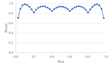
(a) With $\mu=0,\sigma=1,N=5$

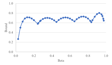
(b) With $\mu=-0.1,\sigma=1,N=5$

4.2.2 Zero Mean

The case with zero mean (i.e., $\mu=\mu^{\prime}-\frac{q}{N}=0$ ) provides invaluable insights into the piece-wise objective function. As a special case of equation (8), we find that (i) the thresholds satisfy $\delta_{k}=\frac{N-k}{N}$ (which is decreasing in $k$) and (ii) the second term on the right-hand side of equation (9) equals zero. We only need to maximize the following expression, which is the first term on the right-hand side of equation (9):

$$T\left(\beta\right)\equiv T\left(k,\beta\right)\equiv N\sigma\sqrt{\beta\left(1-\beta\right)}\frac{\left(N-1\right)!\left(1-\beta\right)^{k-1}\beta^{N-k}}{\left(k-1\right)!\left(N-k\right)!},$$

when $\beta\in\left[\frac{N-k}{N},\frac{N-k+1}{N}\right]$. Each piece $T\left(k,\beta\right)$ is continuous and strictly concave with respect to $\beta$. We obtain the local optimal solution: $\beta_{k}^{\ast}=\frac{2N-2k+1}{2N}$, which is the mid-point of the corresponding interval $\left[\frac{N-k}{N},\frac{N-k+1}{N}\right]$. Substituting the local optimal solution into $T\left(k,\beta\right)$, we obtain the local optimal objective values:

$$T^{\ast}\left(k\right)\equiv T\left(k,\beta_{k}^{\ast}\right)=N\sigma\frac{\left(N-1\right)!\left(\frac{2k-1}{2N}\right)^{k-1}\left(1-\frac{2k-1}{2N}\right)^{N-k}}{\left(k-1\right)!\left(N-k\right)!}\sqrt{\left(\frac{2k-1}{2N}\right)\left(\frac{2N-2k+1}{2N}\right)}.$$ (10)

Lemma 5.

(Local Optimums) With $\mu=0$, the local optimal objective values display the following properties: (i) Symmetric property that $T^{\ast}\left(k\right)=T^{\ast}\left(N-k\right)$ holds for any $k=1,2,...,N$; (ii) Log-convexity with respect to $k$ such that $\max_{k}\left\{T^{\ast}\left(k\right)\right\}=T^{\ast}\left(1\right)=T^{\ast}\left(N\right)$, where

$$T^{\ast}\left(1\right)=T^{\ast}\left(N\right)=N\sigma\left(1-\frac{1}{2N}\right)^{N-1}\sqrt{\frac{1}{2N}\left(1-\frac{1}{2N}\right)}.$$ (11)

As a direct consequence of Lemma 5, we find that with zero mean, it holds that $T(\beta)\leq N\sigma\left(1-\frac{1}{2N}\right)^{N-1}\sqrt{\frac{1}{2N}\left(1-\frac{1}{2N}\right)}$; but there exist two extreme distributions with $\beta=\frac{1}{2N}$ or $\beta=\frac{2N-1}{2N}$ attaining this bound. We illustrate the sequence of $T^{\ast}(k)$ in Figure 2 using $N=5$ and $\sigma=1$. The solid curve depicts the piece-wise objective function while the dashed curve connects all the local peaks as a log-convex curve.

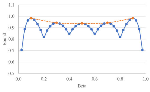
Figure 2: Log-Convexity

4.2.3 Optimal Bound

Equation (9) yields two noteworthy cases: (i) when $\beta\in\left[\delta_{1},1\right]$, we find that

$$Z\left(\beta\right) = Z_{1}\left(\beta\right)\equiv N\mu\left(\sum_{t=1}^{N}\left(\begin{array}[]{c}N\\ t\end{array}\right)\beta^{N-t}\left(1-\beta\right)^{t}\right)+T\left(1,\beta\right)$$

$$= N\mu\left(1-\beta^{N}\right)+N\sigma\sqrt{\beta\left(1-\beta\right)}\beta^{N-1}.$$

since $k=1$, and (ii) when $\beta\in\left[0,\delta_{N-1}\right]$, we find that

$$Z\left(\beta\right) = Z_{N}\left(\beta\right)\equiv N\mu\left(\sum_{t=N}^{N}\left(\begin{array}[]{c}N\\ t\end{array}\right)\beta^{N-t}\left(1-\beta\right)^{t}\right)+T\left(N,\beta\right)$$

$$= N\mu\left(1-\beta\right)^{N}+N\sigma\sqrt{\beta\left(1-\beta\right)}\left(1-\beta\right)^{N-1},$$

since $k=N$. We show that when optimizing the piece-wise objective function $Z\left(\beta\right)$, the optimal solution either falls in the rightmost interval $\left[\delta_{1},1\right]$ or the leftmost interval $\left[0,\delta_{N-1}\right]$ but never falls in the middle. Thus, we either optimize $Z_{1}(\beta)$ or $Z_{N}(\beta)$ to determine the optimal bound. We summarize the results as follows.

Proposition 3.

(Expected Loss) With identical mean and variance, if $\mu<0$, it holds that

$$Z^{\ast}\left(\beta\right)=N\mu+N\hat{\beta}_{1}^{N}\left(-\mu+\sigma\sqrt{\frac{1-\hat{\beta}_{1}}{\hat{\beta}_{1}}}\right),$$

where

$$\hat{\beta}_{1}=\frac{(2N-1)\sigma^{2}+N\mu^{2}-\mu\sqrt{\left(2N-1\right)\sigma^{2}+N^{2}\mu^{2}}}{2N\left(\sigma^{2}+\mu^{2}\right)};$$ (14)

otherwise, if $\mu>0$, then

$$Z^{\ast}\left(\beta\right)=N\left(1-\hat{\beta}_{2}\right)^{N}\left(\mu+\sigma\sqrt{\frac{\hat{\beta}_{2}}{1-\hat{\beta}_{2}}}\right),$$

where

$$\hat{\beta}_{2}=\frac{\sigma^{2}+N\mu^{2}-\mu\sqrt{\left(2N-1\right)\sigma^{2}+N^{2}\mu^{2}}}{2N\left(\sigma^{2}+\mu^{2}\right)}.$$ (15)

Proposition 3 is mainly due to the log-convexity of $T^{\ast}\left(k\right)$. When maximizing a log-convex objective function, the optimal solution must be an extreme point. Interestingly, inequalities (6) imply two extreme points, corresponding to the intervals $\left[\delta_{1},1\right]$ and $\left[0,\delta_{N-1}\right]$. Thus, based on the sign of $\mu$ (i.e., whether $N\mu^{\prime}>q$ or $N\mu^{\prime}<q$), we choose either (14) or (15) to determine the candidate bound on the expected loss.

With non-identical means and variances but under two-point distributions, if $q$ is larger than the total means, then we solve

$$Z=\max_{\beta_{n}}\left\{\sum_{n=1}^{N}\mu_{n}+\left(\Pi_{n=1}^{N}\beta_{n}\right)\cdot\sum_{n=1}^{N}\left(-\mu_{n}+\sigma_{n}\sqrt{\frac{1-\beta_{n}}{\beta_{n}}}\right)\right\}$$ (16)

to obtain the desired bound. Again, we find that the extreme distributions continue to display the equal range property as $\sigma_{n}\left(\sqrt{\frac{\beta_{n}^{\ast}}{1-\beta_{n}^{\ast}}}+\sqrt{\frac{1-\beta_{n}^{\ast}}{\beta_{n}^{\ast}}}\right)=R^{\ast}$ holds.

4.3 Extreme Distribution

A distinguishing feature of our derivation is that both the tail indicator function $\mathbb{I}_{\{X>0\}}$ and linear loss $\max(0,\xi)$ have two linear pieces, making two-point distributions the extreme distributions. We can extend Korkine’s identity to a multi-dimensional environment. Let $\xi_{(i)}=X_{1}+...+X_{N}-X_{i}=\xi-X_{i}$ be the sum excluding the $i$-th random variable and let $X_{i}^{\prime}$ be an independent copy of $X_{i}$, both satisfying the mean-variance conditions. Also denote $\xi^{\prime}=\xi_{(i)}+X_{i}^{\prime}$, meaning that we keep the other $\left(N-1\right)$ random variables intact but randomize the $i$-th random variable one at a time. We observe that

$$\left(\xi-\xi^{\prime}\right)\left(\mathbb{I}_{\{\xi>0\}}-\mathbb{I}_{\{\xi^{\prime}>0\}}\right)=\left(X_{i}-X_{i}^{\prime}\right)\left(\mathbb{I}_{\{X_{i}+\xi_{(i)}>0\}}-\mathbb{I}_{\{X_{i}^{\prime}+\xi_{(i)}>0\}}\right).$$

We define the component summation $T_{i}$ as follows:

$$T_{i}=\mathbb{E}_{\left(X_{i},X_{i}^{\prime},\xi_{(i)}\right)}\left[\left(X_{i}-X_{i}^{\prime}\right)\left(\mathbb{I}_{\{X_{i}+\xi_{(i)}>0\}}-\mathbb{I}_{\{X_{i}^{\prime}+\xi_{(i)}>0\}}\right)\right].$$ (17)

Due to symmetry caused by equal mean and variance, we obtain an intuitive and important relationship as follows.

Lemma 6.

(Total and Component Summations) The total summation $T$ contains $N$ identical component summations, i.e., $T=NT_{i}$.

Lemma 6 implies that

$$\mathbb{E}\left(\xi\right)^{+}=\mathbb{E}\left(\xi\right)\mathbb{E}\left(\mathbb{I}_{\{\xi>0\}}\right)+\frac{1}{2}T=N\mu\Pr\left(\xi>0\right)+\frac{1}{2}NT_{i}.$$

We define the integrand of the component summation as

$$A_{N}=\left|X_{i}-X_{i}^{\prime}\right|\left(\mathbb{I}_{\{\max\left(X_{i},X_{i}^{\prime}\right)+\xi_{(i)}>0\}}-\mathbb{I}_{\{\min\left(X_{i},X_{i}^{\prime}\right)+\xi_{(i)}>0\}}\right),$$

where the subscript $N$ indicates the $N$-dimensional model. We now find that

$$\mathbb{E}\left(\xi\right)^{+}=N\mu\Pr\left(\xi>0\right)+\frac{N}{2}\sum_{X_{i}}\sum_{X_{i}^{\prime}}\sum_{\xi_{(i)}}A_{N}\Pr\left(X_{i}\right)\Pr\left(X_{i}^{\prime}\right)\Pr\left(\xi_{(i)}\right).$$ (18)

An important advantage of equation (18) is that we can derive the $Z(\beta)$ function with fewer steps (see the second proof of Lemma 4 in Appendix A). Equation (18) also has other future applications as it isolates the impact of each individual random variable and bridges between the sum and variance (or absolute deviation) of the random variables.

Theorem 1.

(Extreme Distribution) When determining the upper bound on $\mathbb{E}\left(\xi\right)^{+}$, it suffices to consider only the two-point distributions satisfying equation (4).

To understand the intuition of Theorem 1, we can assume $X_{i}>0>X_{i}^{\prime}$ without loss of generality such that the integrand $A_{N}$ increases along with the absolute value $\left|X_{i}-X_{i}^{\prime}\right|$. The indicator function $\mathbb{I}_{\{X_{i}+\xi_{(i)}>0\}}$ weakly increases with respect to $X_{i}$ and $\xi_{(i)}$. We find that $A_{N}$ must be increasing when $X_{i}^{\prime}$ decreases. Specifically, we find that (i) when $\xi_{(i)}\leq-X_{i}$, $A_{N}=0$ as both indicators are zero; (ii) when $-X_{i}<\xi_{(i)}\leq-X_{i}^{\prime}$, $A=\left(X_{i}-X_{i}^{\prime}\right)$ as the first indicator equals one but the second indicator equals zero; and (iii) when $-X_{i}^{\prime}<\xi_{(i)}$, $A=0$ as both indicators are one. Thus, to increase the integrand, we increase $X_{i}$ but decrease $X_{i}^{\prime}$ as much as possible. By doing so, we also widen the interval $(-X_{i},-X_{i}^{\prime}]$, over which $A_{N}$ is strictly positive, making the expected value $\mathbb{E}\left(A_{N}\right)$ even larger. Therefore, the extreme distributions maximizing $\mathbb{E}\left(\xi\right)^{+}$ must come from the family of two-point distributions. The candidate solutions in Proposition 3 are indeed globally optimal.

4.4 Contrasting with Aggregate Bounds

It is useful to contrast the bounds in Lemma 2 with those in Propositions 1 and 3. Figure 3(a) evaluates the bounds $\frac{\sigma^{2}}{N\left(\mu-\frac{q}{N}\right)^{2}+\sigma^{2}}\allowbreak$ and $\frac{\sigma^{2N}}{\left(\left(\mu-\frac{q}{N}\right)^{2}+\sigma^{2}\right)^{N}}$ using the parameters: $\mu=\sigma=1$ and $q=0.9$. Graphically, the former is higher than the latter; and the gap between them can be visibly wide. Conceptually, the former relaxes the independent constraints, providing an overestimate (underestimate) for the left (right) tail. To highlight the speed of convergence, we also depict the curves (in light grey) based on the normal distribution. Figure 3(a) confirms that relative to normal prior, the bound produced by Proposition 1 on the tail probability is fairly accurate when $N$ increases (while that produced by Lemma 2 is much less accurate).

Using the parameters $\mu^{\prime}=0=\mu-\frac{q}{N}$ and $\sigma=1$, we find that $\mathbb{E}|\xi|=2\mathbb{E}(\xi)^{+}$. Figure 3(b) contains plots of the aggregation bound $\mathbb{E}|\xi|=\sqrt{N^{2}\left(\mu-\frac{q}{N}\right)^{2}+N\sigma^{2}}$ and $2Z_{N}^{\ast}$. Graphically, the former bound is higher than the latter as the former relaxes the independence constraints. In addition to visualization, we also obtain several notable converging results. When each $X_{n}$ follows iid standard normal distributions, we obtain that

$$\mathbb{E}(\xi)^{+}=\frac{1}{\sqrt{2\pi}}\sqrt{N}\approx 0.399\sqrt{N}=0.5\mathbb{E}|\xi|,$$

where $\frac{1}{\sqrt{2\pi}}$ is the standard normal density evaluated at point $x=0$. In contrast, equation (11) yields that

$$\lim_{N\rightarrow\infty}\sqrt{N}\left(1-\frac{1}{2N}\right)^{N-1}\sqrt{\frac{1}{2N}\left(1-\frac{1}{2N}\right)}=\frac{1}{\sqrt{2e}}\approx 0.429,$$

indicating that the improved upper bound on expected loss equals $Z^{\ast}=0.429\sqrt{N}$, which is about $7.5\%$ higher than the exact value under standard normal prior. The aggregation bound on expected loss yields $\bar{Z}=0.5\sqrt{N}$, which is significantly higher than $0.429\sqrt{N}$.

Figure 3: Contrasting with Benchmark

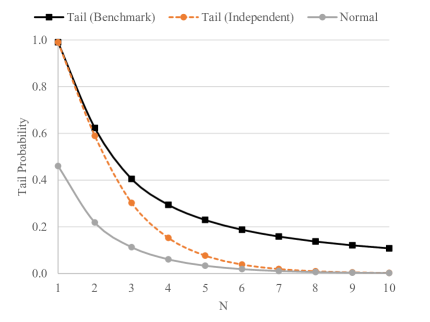
(a) Tail Probability

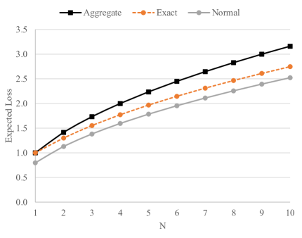
(b) Expected Linear Loss

5 Applications

5.1 Bundle Pricing

Consider the bundle pricing problems.

5.1.1 Equal Mean and Variance

The firm selling $N$ goods in a bundle chooses a posted price $q$ and the customer’s valuation for good $n$ offered in the bundle is $X_{n}$. To ensure that the firm’s ex-post payoff is lower semicontinuous, we assume that only when $X>q$, the customer buys the good; otherwise, the customer walks away. With lower semicontinuity, the bound in Proposition 1 is attained rather than approached. With identical mean and variance, the firm solves the following model:

$$Z=\max_{q}\left\{q-\frac{q\sigma^{2N}}{\left(\left(\mu-\frac{q}{N}\right)^{2}+\sigma^{2}\right)^{N}}\right\}.$$

Corollary 2.

(Pure Bundle Price) Let $t_{N}^{\ast}$ be the root of the polynomial equation:

$$1-2Nt^{2}-\left(t^{2}+1\right)^{N}+t^{2}+2Nt\frac{\mu}{\sigma}-\allowbreak t^{2}\left(t^{2}+1\right)^{N}=0.$$ (19)

Then, the firm’s optimal bundle price is $q_{N}^{\ast}=N\left(\mu-t_{N}^{\ast}\sigma\right)$.

Proof.

We introduce the safety factor $t$ as follows to define the extreme distribution:

$$\left\{\begin{array}[]{l}\Pr\left(\tilde{X}_{i}=\mu-t\sigma\right)=\frac{1}{1+t^{2}}\equiv\beta,\\ \Pr\left(\tilde{X}_{i}=\mu+\frac{1}{t}\sigma\right)=\frac{t^{2}}{1+t^{2}}=1-\beta,\end{array}\right.$$

for each good. We find that for $N\geq 1$, $q=N\left(\mu-t\sigma\right)$ is the bundle price, yielding an expected profit as follows:

$$Z=N(\mu-\sigma t)\left(1-\frac{1}{\left(t^{2}+1\right)^{N}}\right).$$ (20)

When using a component pricing strategy, each product yields an expected profit $Z_{i}=(\mu-\sigma t)\left(1-\frac{1}{t^{2}+1}\right)$. It must hold that

$$Z=N(\mu-\sigma t)\left(1-\frac{1}{\left(t^{2}+1\right)^{N}}\right)\geq N(\mu-\sigma t)\left(1-\frac{1}{t^{2}+1}\right)=NZ_{i},$$

implying that pure bundling is always better than component pricing. To determine the optimal bundle price under independence, we take the first derivative of equation (20) with respect to $t$ as follows:

$$\frac{\partial Z}{\partial t}=\frac{N\sigma}{\left(t^{2}+1\right)^{n}}-N\sigma+2N^{2}t\frac{\mu}{\left(t^{2}+1\right)^{N+1}}-2N^{2}t^{2}\frac{\sigma}{\left(t^{2}+1\right)^{N+1}}=0,$$

which is equivalent to

$$N\sigma\left(1-2Nt^{2}-\left(t^{2}+1\right)^{N}+t^{2}+2Nt\frac{\mu}{\sigma}-\allowbreak t^{2}\left(t^{2}+1\right)^{N}\right)=0.$$

We then confirm Equation (19). ∎

In contrast, if we apply Lemma 2, we solve

$$\tilde{Z}=\max_{q}\left\{q-\frac{q\sigma^{2}}{N\left(\mu-\frac{q}{N}\right)^{2}+\sigma^{2}}\right\}.$$

We obtain a bundle price $\tilde{q}_{N}=N\mu-t^{\#}\sqrt{N}\sigma$, where $t_{N}^{\#}$ solves a cubic equation $t^{3}+3t=\frac{2N\mu}{\sqrt{N}\sigma}=\frac{2\sqrt{N}\mu}{\sigma}$.

Table 2: Bundle Pricing Solutions

$N$	$\tilde{q}_{N}$	$\tilde{Z}_{N}^{\ast}$	$q_{N}^{\ast}$	$Z_{N}^{\ast}$	$\frac{q_{N}^{\ast}-\tilde{q}_{N}}{q_{N}^{\ast}}$	$\frac{Z_{N}^{\ast}-\tilde{Z}_{N}}{Z_{N}^{\ast}}$
$1$	$1.346$	$0.769$	$1.346$	$0.769$	$0.0\%$	$0.0\%$
$2$	$3.000$	$2.000$	$3.000$	$2.250$	$0.0\%$	$11.1\%$
$3$	$4.767$	$3.401$	$4.824$	$3.991$	$1.2\%$	$14.8\%$
$4$	$6.602$	$4.903$	$6.749$	$5.861$	$2.2\%$	$16.3\%$
$5$	$8.484$	$6.476$	$8.741$	$7.811$	$2.9\%$	$17.1\%$
$10$	$18.311$	$14.966$	$19.234$	$18.144$	$4.8\%$	$17.5\%$
$20$	$38.979$	$33.468$	$41.337$	$40.010$	$5.7\%$	$16.4\%$

We contrast the two solutions $\left(\tilde{q}_{N},q_{N}^{\ast}\right)$ and the optimal objective values $\left(\tilde{Z}_{N},Z_{N}^{\ast}\right)$ in Table 2. The parameters include $\mu=2.5$ and $\sigma=1$. As $N$ increases, the gap between $\tilde{q}_{N}$ and $q_{N}^{\ast}$ widens (where $\tilde{q}_{N}$ is consistently lower than $q_{N}^{\ast}$). The gap in the profit is also remarkable, underscoring that independence impacts the quality of the bundle pricing solution.

5.1.2 Unequal Means and Variances

When mean and variance are non-identical across different products, we apply Proposition 2 to define

$$R=\frac{\left(\mu_{n}-q_{n}\right)^{2}+\sigma_{n}^{2}}{\mu_{n}-q_{n}},\text{ for all }n\text{,}$$

as the universal range of all random variables. The firm’s objective function equals

$$Z=\max_{R,q_{n}}\left\{\left(\sum_{n=1}^{N}q_{n}\right)\left[1-\prod_{n=1}^{N}\left(\frac{\sigma_{n}^{2}}{\left(\mu_{n}-q_{n}\right)^{2}+\sigma_{n}^{2}}\right)\right]\right\}.$$ (21)

The constraint on the range $R$ ensures that the internal budget allocation of $q_{n}$ maximizes the product of $\prod_{n=1}^{N}\left(\frac{\sigma_{n}^{2}}{\left(\mu_{n}-q_{n}\right)^{2}+\sigma_{n}^{2}}\right)$. Additionally, the definition of $R$ implies that $q_{n}=-\frac{1}{2}R+\mu_{n}\pm\frac{1}{2}\sqrt{R^{2}-4\sigma_{n}^{2}}$ such that $R\geq 2\sigma_{n}$ must hold. If both roots of $q_{n}$ are positive, we take the smaller root; if there is a negative root, we take the positive root. Due to this inconvenience of having two possible roots, we do not recommend replacing all $q_{n}$ with only one variable $R$. Instead, we endogenously choose $R$ and impose constraints that the range of each random variable must equal $R$.

5.1.3 Mixed Bundle Pricing

In the risk-based model (where the underlying distribution is known), mixed bundle strategies (weakly) outperform pure bundle strategies. Notably, a mixed bundle strategy offers $p_{n}$ for buying only product $n$ and a bundle price $p_{B}$ for buying all the products as a bundle. It usually holds that $p_{B}\leq\sum_{n=1}^{N}p_{n}$ in a mixed bundle strategy. However, in terms of the worst distribution, mixed bundle strategy is equally effective as pure bundle strategy.

Corollary 3.

(Mixed Bundle) When the firm’s objective is to maximize the worst-case expected income, the mixed bundle strategy is equally effective as the pure bundle strategy.

Proof.

As the extreme distribution displays equal range property, we can easily verify that the event $X_{n}>p_{n}$ but $X_{n}+\xi_{(n)}=\xi\leq p_{B}$ occurs with zero probability (i.e., the customer finds that buying only product $n$ gives her the higher utility than buying the bundle). Therefore, the firm’s worst-case expected profit under mixed bundle strategy with $p_{B}$ is identical to that under a pure bundle strategy with $p_{b}$. We conclude that mixed bundle strategy does not improve the firm’s worst-case expected profit when valuations for each good are independent. ∎

Due to Corollary 3, we either apply Proposition 2 or Equation (21) to determine the pure bundle price, depending on whether the mean and variance are identical. This result stands in contrast to Eckalbar, (2010) and Bhargava, (2013) who advocate mixed bundles under uniform distributions. With two products ($N=2$), standard uniform distributions, and zero production costs, both Eckalbar, and Bhargava, show that (i) the optimal mixed bundle is to charge $p_{n}=\frac{2}{3}$ for product $n$ and $p_{B}=\frac{4-\sqrt{2}}{3}$ for both products; and (ii) the pure bundle strategy is to charge $p_{b}=\sqrt{\frac{2}{3}}$ for a pure bundle of both products (i.e., the price for individual product is set at $p_{n}=1$ so that no customer buys only product $n$).

These distribution-specific strategies perform unsatisfactorily under their corresponding extreme distributions with the same mean and variance. Specifically, we use $\mu=0.5$ and $\sigma=\sqrt{\frac{1}{12}}$ as the inputs in our semi-parametric analysis. We find that under mixed or pure bundle strategy where the bundle price is the same (i.e., $p_{B}=p_{b}$), the firm’s most unfavorable distribution remains the same, making the mixed and pure bundle strategies equally effective. The intuition is that the joint distribution forms a square (as suggested by Proposition 2) so that the event a customer buys only product $n$ does not occur in the equilibrium. When $p_{B}=\frac{4-\sqrt{2}}{3}$, the firm’s expected income under the extreme distribution equals merely $0.086$; and when $p_{b}=\sqrt{\frac{2}{3}}$, the firm’s expected income under the extreme distribution equals merely $0.137$. In contrast, when using the robust bundle strategy, the bundle price is $q^{\ast}=0.527$ and the firm’s expected income is $0.338$. Additionally, when $q^{\ast}=0.527$ is used in the uniform distribution, the firm’s expected income equals $0.454$. We observe that the distribution-specific prices are too high while the robust bundle price provides a much better guarantee while the solution based on uniform prior performs unsatisfactorily. Additionally, our method can easily scale to an arbitrary number of products.

5.2 Inventory Management

The firm (that owns a central warehouse) chooses an inventory level $q$ prior to receiving the realized demand $X_{n}$ from retailer $n$. Each retailer is treated equally with the same understocking and overstocking costs $b$ and $h$. Thus, the choice of $q$ is equivalent to choosing a forecast for $\xi$ subject to a generalized linear scoring rule. The ex post loss function equals:

$$Z\left(q,\xi\right)=b\left(\xi-q\right)^{+}+h\left(q-\xi\right)^{+}=\frac{h+b}{2}|\xi-q|+\frac{b-h}{2}\left(\xi-q\right).$$

According to Proposition 3, the firm solves the following model:

$$Z=\min_{q}\left\{\frac{\left(b+h\right)}{2}\max_{\beta}\left[N\mu-q+2\beta^{N}\left(q-N\mu\right)+2N\beta^{N}\sigma\sqrt{\frac{1-\beta}{\beta}}\right]+\frac{\left(b-h\right)}{2}\left(N\mu-q\right)\right\},$$

which represents a zero-sum game between the firm and adverse nature. The firm chooses $q$ to minimize the cost $T(\beta,q)$ but adverse nature chooses $\beta$ to maximize the cost.

Corollary 4.

(Inventory Risk-Pooling) Let $\beta^{\ast}=\left(\frac{b}{b+h}\right)^{\frac{1}{N}}$ be a constant. When $\frac{b}{b+h}\geq\frac{1}{2}$, the firm’s most unfavorable distribution is the following two-point distribution:

$$\left\{\begin{array}[]{l}\Pr\left(\tilde{X}=\mu-\sigma\sqrt{\frac{1-\beta^{\ast}}{\beta^{\ast}}}\right)=\beta^{\ast},\\ \Pr\left(\tilde{X}=\mu+\sigma\sqrt{\frac{\beta^{\ast}}{1-\beta^{\ast}}}\right)=1-\beta^{\ast}.\end{array}\right.$$ (22)

The firm’s optimal inventory level equals:

$$q^{\ast}=N\mu+\sigma\left(\frac{2\beta^{\ast}-1}{2\sqrt{(1-\beta^{\ast})\beta^{\ast}}}-\left(N-1\right)\sqrt{\frac{1-\beta^{\ast}}{\beta^{\ast}}}\right).$$ (23)

The firm’s optimal objective value equals:

$$Z^{\ast}=b\sigma N\sqrt{\frac{1-\beta^{\ast}}{\beta^{\ast}}}.$$ (24)

Proof.

As $\frac{b}{b+h}\geq 0.5$, the firm orders more inventory than the aggregate mean, giving rise to the case of $N\mu<q$. Using the identity that $\left(\xi-q\right)^{+}$ $=\frac{\xi-q}{2}+\frac{1}{2}\left|\xi-q\right|$ and Proposition 3, we find that the payoff function equals

$$Z\left(\beta,q\right)=\frac{\left(b+h\right)}{2}\left[N\mu-q+2\beta^{N}\left(q-N\mu\right)+2N\beta^{N}\sigma\sqrt{\frac{1-\beta}{\beta}}\right]+\frac{\left(b-h\right)}{2}\left(N\mu-q\right).$$

We solve the first-order conditions to determine the saddle point:

$$\frac{\partial Z}{\partial q} = \left(h+b\right)\beta^{N}-b=0$$

$$\frac{\partial Z}{\partial\beta} = \left(h+b\right)\left[N\beta^{N-1}\left(q-N\mu\right)+\frac{N\sigma\beta^{N-1}\left(1-2\beta\right)}{2\sqrt{\left(1-\beta\right)\beta}}+(N-1)N\beta^{N-2}\sigma\sqrt{\left(1-\beta\right)\beta}\right]=0$$

The first condition $\frac{\partial z}{\partial q}=0$ immediately yields Equation (22). With some algebra, we find that the second condition $\frac{\partial Z}{\partial\beta}=0$, along with the newly established Equation (22), yields that

$$\left(q-N\mu\right)2\sqrt{\left(1-\beta\right)\beta}+\sigma\left(1-2\beta\right)+2(N-1)\sigma\left(1-\beta\right)=0.$$

After re-organizing the terms, we confirm Equation (23). Because $\frac{\partial^{2}Z}{\partial q^{2}}=0$, it is easy to verify the second-order conditions to confirm that the pair $(\beta^{\ast},q^{\ast})$ constitutes a saddle point. Finally, substituting $\beta^{\ast}$ and $q^{\ast}$ in to $Z(\beta,q)$, we find that the value of the zero-sum game equals $Z^{\ast}=b\sigma N\sqrt{\frac{1-\beta^{\ast}}{\beta^{\ast}}}$. ∎

In statistical literature, it is known that the linear penalty costs constitute a strictly proper scoring rule for forecasting the percentile (see Theorem 6 in Gneiting and Raftery,, 2007). Hence, the optimal inventory level $q^{\ast}$ shown in Equation (23) is the robust optimal forecast in response to the asymmetric piece-wise linear scoring rule.

If we apply the nonsharp bound in Lemma 2, we solve

$$\tilde{Z}=\min_{q}\left\{\frac{\left(b+h\right)}{2}\sqrt{N^{2}\left(\mu-\frac{q}{N}\right)^{2}+N\sigma^{2}}+\frac{\left(b-h\right)}{2}\left(N\mu-q\right)\right\},$$

and find $\tilde{q}=N\mu+\frac{\sqrt{N}\sigma}{2}\left(\sqrt{\frac{b}{h}}-\sqrt{\frac{h}{b}}\right)$ and $\tilde{Z}=\sigma\sqrt{Nbh}$. We contrast the two solutions $\left(\tilde{q},q^{\ast}\right)$ and the optimal costs $\left(\tilde{Z},Z^{\ast}\right)$ in Table 3. The parameters are $\mu=2.5$, $\sigma=1$, $b=4$, and $h=1$. As $N$ increases, the gap between $\tilde{q}$ and $q^{\ast}$ is moderate (where $\tilde{q}$ is consistently higher than $q^{\ast}$). The gap in terms of the expected cost is more visible (which is as high as $5.6\%$), underscoring that independence impacts the quality of the inventory solution.

Table 3: Inventory Solutions

$N$	$\tilde{q}$	$\tilde{T}$	$q^{\ast}$	$T^{\ast}$	$\frac{\tilde{q}-q^{\ast}}{q^{\ast}}$	$\frac{\tilde{T}-T^{\ast}}{T^{\ast}}$
$1$	$3.250$	$2.000$	$3.250$	$2.000$	$0.0\%$	$0.0\%$
$2$	$6.061$	$2.828$	$5.940$	$2.748$	$2.0\%$	$2.9\%$
$3$	$8.799$	$3.464$	$8.605$	$3.335$	$2.3\%$	$3.9\%$
$4$	$11.500$	$4.000$	$11.249$	$3.832$	$2.2\%$	$4.4\%$
$5$	$14.177$	$4.472$	$13.879$	$4.273$	$2.1\%$	$4.7\%$
$10$	$27.372$	$6.325$	$26.901$	$6.009$	$1.7\%$	$5.3\%$
$20$	$53.354$	$8.944$	$52.655$	$8.474$	$1.3\%$	$5.6\%$

5.3 Option Pricing

Suppose that the price change of a trading asset in day $n$ from the starting value of zero is $X_{n}$. Thus, after $N$ trading days, the price of the asset becomes $\xi=X_{1}+X_{2}+\ldots+X_{N}$. For simplicity, we assume that the asset brings no dividends and consider an European call option on this asset with strike price $q$ and maturity in $N$ days. The expected pay-off of the option is $\mathbb{E}\left(\xi-q\right)^{+}$ and risk-neutral price is $e^{-rN}\mathbb{E}\left(\xi-q\right)^{+}$, where $r$ is the risk-free rate. Lo, (1987) proved the following sharp bounds

$$\mathbb{E}\left(\xi-q\right)^{+}\leq\mu-q\frac{\mu^{2}}{\mu^{2}+\sigma^{2}},\text{ if }q\leq\frac{\mu^{2}+\sigma^{2}}{2\mu}$$

and

$$\mathbb{E}\left(\xi-q\right)^{+}\leq\frac{1}{2}(\mu-q+\sqrt{(q-\mu)^{2}+\sigma^{2}}),\text{ otherwise.}$$

The last bound coincided with the benchmark established in Lemma 2 of Section 2.2.

Instead of using simulations from a specified parametric distribution (which is very restrictive as an incorrect prior distribution can cause significant loss, for instance, in the bundle pricing example), the improved bounds in Propositions 1 and 3 are essential for valuation of options since traders need to estimate the probability of reaching the strike price $\xi>0$ (price higher than the current price) and to assess $\mathbb{E}\left|\xi\right|$. Both bounds are clearly important for valuation of options. While Cox et al., (1979) developed the option pricing model based on Binomial distributions, Proposition 3 implies that such a result constitutes an upper bound estimate on $\mathbb{E(}\xi)^{+}$.

To incorporate unequal mean and variance (i.e., the scenario of price shocks or price dynamics), we can apply Equation (16) to choose the parameters as the input data for the Binomial option pricing model that Cox et al., (1979) study. The equal range property ensures that the lattices are squares with the same size despite unequal mean and variance. As Table 1 indicated, we can interpret $\xi$ as the aggregate claim of multiple property damages and then the bound on $\mathbb{E(}\xi)^{+}$ provides an upper bound estimate of the expected aggregate claim.

In an applied example, we consider the share price of National Australia Bank Ltd. (NAB.ASX). We use the data from 10 May to 17 November 2023 as the training data to compute the mean and standard deviation. This training period happens to exclude any dividend. The average price change on each trading day is $0.0194$ Australian dollar and standard deviation is $0.2752$ Australian dollar. As at 10 May, the closing price is $26.26$. We set the strike price at $q=28.8$. We also include the normal prior benchmark and set the discount rate at $r=0$ for convenience. We compute the price for an European call option with different expiration days, reported in Table 4.

Table 4: Option Prices of NAB Ltd.

Strike Price $q=28.8$	$N=10$	$N=30$	$N=60$	$N=100$	$N=200$
Aggregation	$0.078$	$0.256$	$0.580$	$1.108$	$2.727$
Improved	$0.077$	$0.245$	$0.532$	$0.971$	$2.572$
Normal Prior	$0.001$	$0.069$	$0.333$	$0.823$	$2.313$

A quick observation is that the aggregation bound proposed by Lo, (1987) tends to overprice the European call option (as the second row of Table 4 indicated). The closed form expression and high accuracy make Proposition 3 an attractive alternative to many standard convex algorithms (see Henrion et al.,, 2023, for updated literature in this area). In general, Equation (14) is more suitable for call European options as the strike price is often higher than the mean while Equation (15) is more suitable for put European options as the strike price is often lower than the mean.

6 Conclusion

We develop two sets of results associated with the sum of independent random variables using only the mean and variance. The results complement earlier Chebyshev-type results such as Bentkus, (2004), de la Peña et al., (2004), and Yang and Mo, (1985) and provide important new insights, proof strategies and tighter bounds than those obtained by aggregation. We show significant improvements arising from using the new bounds in such popular applications as bundle pricing, inventory management and option pricing.

Appendix: Proofs Related to Section 4

Proof of Lemma 3:

As a direct result of Corollary 1, it must hold that $\mu-\sigma\sqrt{\frac{1-\beta}{\beta}}\leq 0\leq\mu+\sigma\sqrt{\frac{\beta}{1-\beta}}$ (otherwise $\beta=\Pr\left(X\leq 0\right)$ cannot be feasible). Under the extreme distribution in Equation (4), the integrand $A_{1}$ equals zero if $X=X^{\prime}$; otherwise, $A_{1}$ equals $H-L=\sigma\sqrt{\frac{\beta}{1-\beta}}+\sigma\sqrt{\frac{1-\beta}{\beta}}=\sigma\sqrt{\beta(1-\beta)}$, which is the range of the two-point distribution. We confirm that the summation equals

$$T = \sum_{X}\sum_{X^{\prime}}\left[\left(X-X^{\prime}\right)\left(\mathbb{I}_{\{X>0\}}-\mathbb{I}_{\{X^{\prime}>0\}}\right)\right]\Pr\left(X\right)\Pr\left(X^{\prime}\right)$$

$$= 2\left(\sigma\sqrt{\frac{\beta}{1-\beta}}+\sigma\sqrt{\frac{1-\beta}{\beta}}\right)\beta\left(1-\beta\right)=2\sigma\sqrt{\beta-\beta^{2}},$$

yielding inequality (5). $\blacksquare$

Proof of Lemma 4:

We provide two different proofs of Lemma 4. The first proof directly uses the probability mass function of the endogenous Binomial distribution while the second proof uses Korkine’s identity.

Proof.

Using the definition of $\delta_{k}$ and the probability mass function in (7), we find that

$$\mathbb{E}(\xi)^{+}\equiv Z\left(\beta\right)=\sum_{t=k}^{N}\left[N\mu+\sigma\left(-\left(N-t\right)\sqrt{\frac{1-\beta}{\beta}}+t\sqrt{\frac{\beta}{1-\beta}}\right)\right]\frac{N!\left(1-\beta\right)^{t}\beta^{N-t}}{t!(N-t)!}.$$

We define a sequence of $\left\{y_{t}\right\}$ as follows. For $t=N$, it holds that

$$y_{N}=N\sqrt{\frac{\beta}{1-\beta}}\left(1-\beta\right)^{N}=N\left(1-\beta\right)^{N-1}\sqrt{\beta\left(1-\beta\right)}.$$

For $t\leq N-1$, it holds that

$$y_{t} = \left(-\left(N-t\right)\sqrt{\frac{1-\beta}{\beta}}+t\sqrt{\frac{\beta}{1-\beta}}\right)\frac{N!\left(1-\beta\right)^{t}\beta^{N-t}}{t!(N-t)!}$$

$$= -\left(N-t\right)\sqrt{\frac{1-\beta}{\beta}}\frac{N!\left(1-\beta\right)^{t}\beta^{N-t}}{t!(N-t)!}+t\sqrt{\frac{\beta}{1-\beta}}\frac{N!\left(1-\beta\right)^{t}\beta^{N-t}}{t!(N-t)!}$$

$$= -N\sqrt{\beta\left(1-\beta\right)}\frac{\left(N-1\right)!\left(1-\beta\right)^{t}\beta^{N-t-1}}{t!(N-t-1)!}+N\sqrt{\beta\left(1-\beta\right)}\frac{\left(N-1\right)!\left(1-\beta\right)^{t-1}\beta^{N-t}}{\left(t-1\right)!(N-t)!}.$$

Contrasting $y_{t}$ and $y_{t+1}$ (for $t\leq N-1$), we find that the negative term of $y_{t}$ equals the positive term of $y_{t+1}$. Hence, the summation equals

$$y_{k}+y_{k+1}+...+y_{N}$$

$$= -N\sqrt{\beta\left(1-\beta\right)}\frac{\left(N-1\right)!\left(1-\beta\right)^{k}\beta^{N-k-1}}{k!(N-k-1)!}+N\sqrt{\beta\left(1-\beta\right)}\frac{\left(N-1\right)!\left(1-\beta\right)^{k-1}\beta^{N-k}}{\left(k-1\right)!(N-k)!}$$

$$-N\sqrt{\beta\left(1-\beta\right)}\frac{\left(N-1\right)!\left(1-\beta\right)^{k+1}\beta^{N-k-2}}{(k+1)!(N-k-2)!}+N\sqrt{\beta\left(1-\beta\right)}\frac{\left(N-1\right)!\left(1-\beta\right)^{k}\beta^{N-k-1}}{k!(N-k-1)!}$$

$$...-N\sqrt{\beta\left(1-\beta\right)}\frac{\left(N-1\right)!\left(1-\beta\right)^{N-1}}{(N-1)!}+N\sqrt{\beta\left(1-\beta\right)}\frac{\left(N-1\right)!\left(1-\beta\right)^{N-2}\beta}{(N-2)!1!}$$

$$+N\left(1-\beta\right)^{N-1}\sqrt{\beta\left(1-\beta\right)}$$

$$= N\sqrt{\beta\left(1-\beta\right)}\frac{\left(N-1\right)!\left(1-\beta\right)^{k-1}\beta^{N-k}}{\left(k-1\right)!(N-k)!},$$

whereby only the positive term of $y_{t}$ is not cancelled out. Thus, the expected loss equals

$$Z\left(\beta\right) = \sigma\left(y_{k}+y_{k+1}+...+y_{N}\right)+N\mu\sum_{t=k}^{N}\frac{N!\left(1-\beta\right)^{t}\beta^{N-t}}{t!(N-t)!}$$

$$= N\sigma\sqrt{\beta\left(1-\beta\right)}\frac{\left(N-1\right)!\left(1-\beta\right)^{k-1}\beta^{N-k}}{\left(k-1\right)!(N-k)!}+N\mu\sum_{t=k}^{N}\frac{N!\left(1-\beta\right)^{t}\beta^{N-t}}{t!(N-t)!},$$

which proves Equation (9). ∎

Proof.

We apply Equation (18) to compute the expected loss under the endogenous Binomial distribution. We observe that if $\beta\in\left[\delta_{k},\delta_{k-1}\right]$, $\left(N-t\right)L+tH$ is positive for $t\geq k$ but is negative for $t\leq k-1$. Thus, when $\xi_{(i)}=\left(N-k\right)L+\left(k-1\right)H$, it holds that $H+\xi_{(i)}=\left(N-k\right)L+kH>0$ and $L+\xi_{(i)}=\left(N-k+1\right)L+\left(k-1\right)H\leq 0$. The coefficient equals $\left(\mathbb{I}_{\{H+\xi_{(i)}>0\}}-\mathbb{I}_{\{L+\xi_{(i)}>0\}}\right)=1$. This event occurs with probability $\frac{(N-1)!\left(1-\beta\right)^{k-1}\beta^{N-k}}{(k-1)!(N-k)!}$. For all the other $\xi_{(i)}\neq\left(N-k\right)L+\left(k-1\right)H$, the two indicators have the same value, making the coefficient $\left(\mathbb{I}_{\{H+\xi_{(i)}>0\}}-\mathbb{I}_{\{L+\xi_{(i)}>0\}}\right)=0$. Hence, we find that when $\beta\in\left[\delta_{k},\delta_{k-1}\right]$, Equation (18) equals

$$Z\left(\beta\right) = N\mu\sum_{t=k}^{N}\frac{N!\beta^{N-t}\left(1-\beta\right)^{t}}{t!\left(N-t\right)!}$$

$$+\frac{N}{2}2\sigma\left(\sqrt{\frac{\beta}{1-\beta}}+\sqrt{\frac{1-\beta}{\beta}}\right)\beta\left(1-\beta\right)\frac{\left(N-1\right)!\left(1-\beta\right)^{k-1}\beta^{N-k}}{\left(k-1\right)!\left(N-k\right)!},$$

which is identical to Equation (9). ∎

Proof of Lemma 5:

We recall that over the interval $\left[\delta_{k},\delta_{k-1}\right]$, the piece-wise objective function equals

$$T\left(k,\beta\right)=N\sigma\sqrt{\beta\left(1-\beta\right)}\frac{\left(N-1\right)!\left(1-\beta\right)^{k-1}\beta^{N-k}}{\left(k-1\right)!\left(N-k\right)!}.$$

It is more convenient to take logarithm and consider $\ln(T(k,\beta))=\ln(N\sigma)+\left(k-\frac{1}{2}\right)\ln\left(1-\beta\right)+\left(N-k+\frac{1}{2}\right)\ln\beta$. The first order condition yields that

$$\frac{\partial\ln T\left(k,\beta\right)}{\partial\beta}=-\frac{\left(2N-2k-2N\beta+1\right)}{2\beta\left(\beta-1\right)}=0,$$

indicating that $\beta_{k}^{\ast}=\frac{1}{2N}\left(2N-2k+1\right)$. Substituting $\beta_{k}^{\ast}$ into $T\left(k,\beta\right)$, we obtain the local optimal objective value $T^{\ast}\left(k\right)$ shown in Equation (10). The second order condition yields that

$$\frac{\partial^{2}\ln T\left(k,\beta\right)}{\partial\beta^{2}}=-\frac{1}{2\beta^{2}\left(\beta-1\right)^{2}}\left(2N-2k-2\beta-4N\beta+4k\beta+2N\beta^{2}+1\right).$$

The numerator is a convex and quadratic function with respect to $\beta$. The determinant of this quadratic equation equals

$$\Delta=\left(-2-4N+4k\right)^{2}-4\cdot 2N\cdot\left(2N-2k+1\right)=-4\left(2k-1\right)\left(2N-2k+1\right)\allowbreak<0$$

due to $1\leq k\leq N$. Thus, the numerator is always positive, meaning that $\frac{\partial^{2}\ln T\left(k,\beta\right)}{\partial\beta^{2}}<0$ and making $\ln T\left(k,\beta\right)$ a log-concave function with respect to $\beta$. We conclude that $\beta_{k}^{\ast}=\frac{1}{2N}\left(2N-2k+1\right)$ is a local optimal solution over the interval $\left[\delta_{k},\delta_{k-1}\right]$.

(i) The symmetry property as illustrated in Figure 1(a) is trivial due to the relationship

$$\beta_{k}^{\ast}=\frac{1}{2N}\left(2N-2k+1\right)=1-\frac{1}{2N}\left(2N-2\left(N-k\right)+1\right)=\allowbreak 1-\beta_{N-k}^{\ast}$$

and the symmetry of $T\left(k,\beta\right)=T\left(N-k,1-\beta\right)$.

(ii) To prove the log-convex property, we take logarithm such that

$$\ln T_{k} = \ln\Gamma\left(N\right)-\ln\Gamma\left(k\right)-\ln\Gamma\left(N-k+1\right)$$

$$+\left(k-\frac{1}{2}\right)\ln\left(\frac{2k-1}{2N}\right)+\left(N-k+\frac{1}{2}\right)\ln\left(1-\frac{2k-1}{2N}\right),$$

where $\Gamma\left(k\right)=\left(k-1\right)!$ is the Gamma function. Since

$$\frac{\partial^{2}}{\partial k^{2}}\left(\left(k-\frac{1}{2}\right)\ln\left(\frac{2k-1}{2N}\right)+\left(N-k+\frac{1}{2}\right)\ln\left(1-\frac{2k-1}{2N}\right)\right)=\frac{1}{k-\frac{1}{2}}+\frac{1}{N-k+\frac{1}{2}},$$

and $\ln\Gamma\left(N\right)$ is a constant, our task is to show that

$$G=\frac{\partial^{2}\ln\Gamma\left(k\right)}{\partial k^{2}}+\frac{\partial^{2}\ln\Gamma\left(N-k+1\right)}{\partial k^{2}}<\frac{1}{k-\frac{1}{2}}+\frac{1}{N-k+\frac{1}{2}}.$$

It is known that $\frac{\partial^{2}\ln\Gamma\left(k\right)}{\partial k^{2}}=\psi^{(1)}\left(k\right)$ is the Trigamma function satisfying $\psi^{(1)}\left(k\right)\approx\frac{1}{k}+\frac{1}{2k^{2}}+\frac{1}{6k^{3}}-\frac{1}{30x^{5}}+...$. As the fourth term has a negative coefficient, we use the first three terms of the expansion to construct an upper bound on $G$ as follows:

$$G\leq\frac{1}{k}+\frac{1}{2k^{2}}+\frac{1}{6k^{3}}+\frac{1}{N-k+1}+\frac{1}{\left(N-k+1\right)^{2}}+\frac{1}{6\left(N-k+1\right)^{3}},$$

which is consistent with Theorem 4 in Gordon, (1994). Due to symmetry, it suffices to show that

$$\frac{1}{k}+\frac{1}{2k^{2}}+\frac{1}{6k^{3}}-\frac{1}{k-\frac{1}{2}}=-\frac{k+1}{6k^{3}\left(2k-1\right)}<0,$$

for any $1\leq k\leq N$. We conclude that $G<\frac{1}{k-\frac{1}{2}}+\frac{1}{N-k+\frac{1}{2}}$, which ensures that $\frac{\partial^{2}}{\partial k^{2}}\left(\ln(T_{k})\right)>0$. $\blacksquare$

Proof of Proposition 3:

When optimizing $Z_{1}(\beta)$, we solve the following first order condition:

$$\frac{\partial Z_{1}\left(\beta\right)}{\partial\beta} = \frac{\partial}{\partial\beta}\left(N\mu\left(1-\beta^{N}\right)+N\sigma\sqrt{\beta\left(1-\beta\right)}\beta^{N-1}\right)$$

$$= -\frac{N\beta^{N-1}}{2\sqrt{\beta\left(1-\beta\right)}}\left(\sigma-2N\sigma+2N\sigma\beta+2N\mu\sqrt{\beta\left(1-\beta\right)}\right)=0,$$

which results in Equation (14). The candidate solution $\hat{\beta}_{1}$ is in the interior of $\left[\delta_{1},1\right]$, meaning that

$$-\left(N-1\right)\sigma\sqrt{\frac{1-\hat{\beta}_{1}}{\hat{\beta}_{1}}}+\sigma\sqrt{\frac{\hat{\beta}_{1}}{1-\hat{\beta}_{1}}}>0.$$

Thus, under $\hat{\beta}_{1}$, only when all $X_{n}=\mu-\sigma\sqrt{\frac{1-\hat{\beta}_{1}}{\hat{\beta}_{1}}}$, can the sum $\xi$ be negative. The expected loss indeed equals $Z^{\ast}=N\mu-N\hat{\beta}_{1}^{N}\left(\mu-\sigma\sqrt{\frac{1-\hat{\beta}_{1}}{\hat{\beta}_{1}}}\right)$ under this extreme two-point distribution. Similarly, by optimizing $Z_{N}\left(\beta\right)$ we solve the following first order condition:

$$\frac{\partial Z_{N}\left(\beta\right)}{\partial\beta} = \frac{\partial}{\partial\beta}\left(N\mu\left(1-\beta\right)^{N}+N\sigma\sqrt{\beta\left(1-\beta\right)}\left(1-\beta\right)^{N-1}\right)$$

$$= -\frac{N\left(1-\beta\right)^{N}\sqrt{\beta\left(1-\beta\right)}}{2\beta\left(1-\beta\right)^{2}}\left(2N\sigma\beta-\sigma+2N\mu\sqrt{\beta\left(1-\beta\right)}\right)=0,$$

which results in Equation (15).

Next, we investigate the sign of $g\left(\mu\right)=\frac{1}{N}\left(Z_{1}(\hat{\beta}_{1})-Z_{N}(\hat{\beta}_{N})\right)$. When $\mu=0$, Lemma 5 has shown that $g\left(0\right)=0$. Applying the envelope theorem, we find that

$$g^{\prime}\left(\mu\right)=\frac{1}{N}\frac{\partial Z_{1}(\beta)}{\partial\mu}|_{\beta=\hat{\beta}_{1}}-\frac{1}{N}\frac{\partial Z_{N}(\beta)}{\partial\mu}|_{\beta=\hat{\beta}_{N}}=1-\hat{\beta}_{1}^{N}-\left(1-\hat{\beta}_{N}\right)^{N}.$$

At the point $\mu=0$, it holds that

$$g^{\prime}\left(\mu\right)|_{\mu=0}=1-\left(\frac{2N-1}{2N}\right)^{N}-\left(1-\frac{1}{2N}\right)^{N}<0.$$

Thus, when $\Delta\mu>0$ (which occurs when $\mu$ increases from zero to a positive number), $g\left(\mu\right)\simeq\left[g^{\prime}\left(\mu\right)|_{\mu=0}\right]\Delta\mu<0$, suggesting that $Z_{1}(\hat{\beta}_{1})-Z_{N}(\hat{\beta}_{N})<0$, making $\hat{\beta}_{N}$ a better solution than $\hat{\beta}_{1}$. Likewise, when $\Delta\mu<0$ (which occurs when $\mu$ decreases from zero to a negative number), $g\left(\mu\right)\simeq\left[g^{\prime}\left(\mu\right)|_{\mu=0}\right]\Delta\mu>0$, suggesting that $Z_{1}(\hat{\beta}_{1})-Z_{N}(\hat{\beta}_{N})>0$, making $\hat{\beta}_{1}$ a better solution than $\hat{\beta}_{N}$.

Using the same method, we can contrast $\max\left\{Z_{1}(\hat{\beta}_{1}),Z_{N}(\hat{\beta}_{N})\right\}$ with any other local optimum objective value $Z_{k}(\hat{\beta}_{k})$, where $k\in\left\{2,3,...,N-1\right\}$. We notice that

$$Z_{k}\left(\beta\right) = \frac{N!}{(N-k)!(k-1)!}\sigma\sqrt{\beta(1-\beta)}(1-\beta)^{k-1}\beta^{N-k}$$

$$+N\mu\left(1-\beta^{N}-N\beta^{N-1}(1-\beta)-...-\frac{N!}{(N-k+1)!(k-1)!}\beta^{N-k+1}(1-\beta)^{k-1}\right).$$

The first order condition yields that

$$\frac{\partial Z_{k}\left(\beta\right)}{\partial\beta}=-\frac{\sigma}{2}\frac{N!\beta^{N-k+1}\left(1-\beta\right)^{k-1}}{(N-k)!(k-1)!\sqrt{\beta\left(1-\beta\right)}}\left[\left(2k-1\right)\sigma-2N\sigma+2N\sigma\beta+2N\mu\sqrt{\beta\left(1-\beta\right)}\right]=0.$$

Thus, we find that

$$\hat{\beta}_{k}=\frac{\sigma^{2}\left(2N-2k+1\right)+N\mu^{2}-\mu\sqrt{N^{2}\mu^{2}+\sigma^{2}\left(2k-1\right)\left(2N-2k+1\right)}}{2N\left(\sigma^{2}+\mu^{2}\right)}.$$

In a special case with $\mu=0$, we recover the same result in the proof of Lemma 5 that $\hat{\beta}_{k}=\frac{2N-2k+1}{2N}$. When $\mu<0$ (which implies $\Delta\mu<0$), we find that

$$\frac{1}{N}\frac{\partial}{\partial\mu}Z_{k}(\hat{\beta}_{k})|_{\mu=0} = 1-\hat{\beta}_{k}^{N}-N\hat{\beta}_{k}^{N-1}(1-\hat{\beta}_{k})-...-\frac{N!}{(N-k+1)!(k-1)!}\hat{\beta}_{k}^{N-k+1}(1-\hat{\beta}_{k})^{k-1}$$

$$= 1-\left(\frac{2N-2k+1}{2N}\right)^{N}-...-\frac{N!}{(N-k+1)!(k-1)!}\left(\frac{2N-2k+1}{2N}\right)^{N-k+1}\left(\frac{2k-1}{2N}\right)^{k-1}$$

$$> 1-\left(\frac{2N-1}{2N}\right)^{N}=\frac{\partial}{\partial\mu}Z_{1}(\hat{\beta}_{1})|_{\mu=0}.$$

At the point $\mu=0$, Lemma 5 already shows that $Z_{1}(\hat{\beta}_{1})>Z_{k}(\hat{\beta}_{k})$. We find that $Z_{1}(\hat{\beta}_{1})-Z_{k}(\hat{\beta}_{k})\simeq\frac{\partial}{\partial\mu}\left(Z_{1}(\hat{\beta}_{1})-Z_{k}(\hat{\beta}_{k})\right)|_{\mu=0}\Delta\mu>0$, making $\hat{\beta}_{1}$ the global optimal solution for $Z\left(\beta\right)$ when $\mu<0$. Similarly, we find that when $\mu>0$, $Z_{N}(\hat{\beta}_{N})>Z_{k}(\hat{\beta}_{k})$.

In summary, the global optimal solution is 1) $\hat{\beta}_{1}$ when $\mu<0$ or 2) $\hat{\beta}_{N}$ when $\mu>0$. Certainly, Lemma 5 already shows that when $\mu=0$, there exist two global optimal solutions $\hat{\beta}_{1}=\frac{2N-1}{2N}$ and $\hat{\beta}_{N}=\frac{1}{2N}$. $\blacksquare$

References

- Axaster, (2000) Axaster, S. (2000). Inventory Control. Springer, London, United Kingdom.
- Azuma, (1967) Azuma, K. (1967). Weighted sums of certain dependent random variables. Tohoku Mathematical Journal, 19(3):357–367.
- Bentkus, (2004) Bentkus, V. (2004). On Hoeffding’s inequalities. The Annals of Probability, 32(2):1650 – 1673.
- Bernshtein, (1946) Bernshtein, S. (1946). Theory of probability. Gostekhizdat, Moscow.
- Bhargava, (2013) Bhargava, H. K. (2013). Mixed bundling of two independently valued goods. Management Science, 59(9):2170–2185.
- Billingsley, (1995) Billingsley, P. (1995). Probability and Measure. Wiley Series in Probability and Statistics. Wiley.
- Chernoff, (1952) Chernoff, H. (1952). A measure of asymptotic efficiency for tests of a hypothesis based on the sum of observations. The Annals of Mathematical Statistics, 23(4):493 – 507.
- Cox et al., (1979) Cox, J. C., Ross, S. A., and Rubinstein, M. (1979). Option pricing: a simplified approach. Journal of Financial Economics, 7(3):229–263.
- de la Peña, (1999) de la Peña, V. H. (1999). A general class of exponential inequalities for martingales and ratios. The Annals of Probability, 27(1):537–564.
- de la Peña et al., (2004) de la Peña, V. H., Ibragimov, R., and Jordan, S. (2004). Option bounds. Journal of Applied Probability, 41(A):145–156.
- de la Peña et al., (2009) de la Peña, V. H., Lai, T. L., and Shao, Q.-M. (2009). Self-Normalized Processes: Limit Theory and Statistical Applications. Springer Berlin Heidelberg, Berlin, Heidelberg.
- Eckalbar, (2010) Eckalbar, J. C. (2010). Closed-form solutions to bundling problems. Journal of Economics & Management Strategy, 19(2):513–544.
- Freedman, (1975) Freedman, D. A. (1975). On Tail Probabilities for Martingales. The Annals of Probability, 3(1):100 – 118.
- Gneiting and Raftery, (2007) Gneiting, T. and Raftery, A. E. (2007). Strictly proper scoring rules, prediction, and estimation. Journal of the American Statistical Association, 102(477):359–378.
- Gordon, (1994) Gordon, L. (1994). A stochastic approach to the gamma function. The American Mathematical Monthly, 101(9):858–865.
- Henrion et al., (2023) Henrion, D., Kirschner, F., De Klerk, E., Korda, M., Lasserre, J.-B., and Magron, V. (2023). Revisiting semidefinite programming approaches to options pricing: Complexity and computational perspectives. INFORMS Journal on Computing, 35(2):335–349.
- Hoeffding, (1963) Hoeffding, W. (1963). Probability inequalities for sums of bounded random variables. Journal of the American Statistical Association, 58(301):13–30.
- Lo, (1987) Lo, A. W. (1987). Semi-parametric upper bounds for option prices and expected payoffs. Journal of Financial Economics, 19(2):373–387.
- Mallows, (1956) Mallows, C. L. (1956). Generalizations of Tchebycheff’s inequalities. Journal of the Royal Statistical Society: Series B (Methodological), 18(2):139–168.
- Marinelli, (2024) Marinelli, C. (2024). On some semi-parametric estimates for european option prices. Journal of Applied Probability, page 1–11.
- Mattner, (2003) Mattner, L. (2003). Mean absolute deviations of sample means and minimally concentrated binomials. The Annals of Probability, 31(2):914 – 925.
- McDiarmid, (1989) McDiarmid, C. (1989). On the method of bounded differences. In Surveys in Combinatorics, London Mathematical Society Lectures Notes 141, pages 148–188. Cambridge University Press, Cambridge, UK.
- Mitrinović et al., (1993) Mitrinović, D., Pečarić, J. E., and Fink, A. M. (1993). Classical and New Inequalities in Analysis. Kluwer Academic Publishers, Springer Dordrecht, Amsterdam.
- Pinelis, (1994) Pinelis, I. (1994). Optimum bounds for the distributions of martingales in banach spaces. The Annals of Probability, 22(4):1679 – 1706.
- Scarf, (1958) Scarf, H. (1958). A min-max solution of an inventory problem. Studies in the Mathematical Theory of Inventory and Production, 10(2):201–209.
- Yang and Mo, (1985) Yang, M. C. K. and Mo, T. C. (1985). Distribution-free confidence bounds for . Journal of the American Statistical Association, 80(389):227–230.