Optimal Batch Allocation for Wireless Federated Learning
Abstract
Federated learning aims to construct a global model that fits the dataset distributed across local devices without direct access to private data, leveraging communication between a server and the local devices. In the context of a practical communication scheme, we study the completion time required to achieve a target performance. Specifically, we analyze the number of iterations required for federated learning to reach a specific optimality gap from a minimum global loss. Subsequently, we characterize the time required for each iteration under two fundamental multiple access schemes: time-division multiple access (TDMA) and random access (RA). We propose a step-wise batch allocation, demonstrated to be optimal for TDMA-based federated learning systems. Additionally, we show that the non-zero batch gap between devices provided by the proposed step-wise batch allocation significantly reduces the completion time for RA-based learning systems. Numerical evaluations validate these analytical results through real-data experiments, highlighting the remarkable potential for substantial completion time reduction.
Index Terms:
Batch allocation, federated learning, multiple access, wireless distributed learning.I Introduction
The rapid advancement of Internet of Things (IoT) technology has led to an explosive increase in the number of IoT devices. It is estimated that the number of IoT connections will surpass 34 billion by 2023, according to Ericsson’s recent report [1]. This exponential growth in IoT devices has resulted in the generation of vast volumes of data. Simultaneously, the dramatic evolution of machine learning techniques, particularly in the realm of artificial intelligence (AI), has opened new avenues for harnessing the wealth of data generated by these devices.
However, due to the vast scale of IoT datasets, constructing a single centralized machine for storage and processing becomes impractical. Furthermore, numerous types of data generated by IoT, such as financial and health information, are personal and highly sensitive. This naturally results in data owners being hesitant to grant access to centralized entities. To address such challenges of handling large-scale data while preserving data privacy, federated learning has emerged as a promising solution [2]. In a federated learning system, a central server coordinates the learning process, while local devices compute models, i.e., artificial neural network models, using their own locally stored data. Importantly, no data is exchanged between the server and the devices. Instead, the local models computed by the devices are transmitted to the server. Upon receiving these local models, the server aggregates them to produce a global model, which is subsequently sent back to the devices for the next iteration. This iterative process continues, ultimately resulting in the training of the global model.
One of the key advantages of federated learning is that it does not require direct access to local data. The server constructs the global model by aggregating local models, making it well-suited for applications involving sensitive or private data. Furthermore, since the entire dataset is distributed across numerous devices, the computational load on each device is substantially lower than that in centralized learning. This distributed nature of federated learning also enables the exploitation of parallel computing techniques [3].
However, a limitation of federated learning is that no single entity can access the entire dataset. Consequently, updating the global model in each iteration may be less efficient compared to centralized counterparts, often requiring more iterations to achieve the desired performance. Additionally, communication is essential in each iteration, as local models must be transmitted from the devices to the server, and the updated global model is sent from the server to the devices. This communication overhead can become a bottleneck in federated learning [4].
In response to these challenges, researchers have focused on developing communication-efficient federated learning techniques. Notable approaches include Federated Averaging (FedAvg), which aggregates local models from a subset of devices to reduce communication overhead [2]. Moreover, in [5], the authors have proposed an updates scheme that compresses parameters of local models to reduce communication cost. In addition, strategies involving periodic transmission of local models have been proposed in [6, 7] to decrease communication frequency. Some methods have even leveraged primal-dual optimization techniques to further reduce communication requirements [8].
Another approach seeks to minimize the number of communications by introducing event-triggered aggregation, where local models are sent to the server only when the difference between the most recently sent model and the current local model exceeds a predefined threshold [9]. This approach aligns with the development of decentralized systems that address optimization problems in a distributed manner [10].
In addition to that, another line of research focuses on resource optimization for enhancing bandwidth and energy efficiency. Energy-efficient strategies have considered the amount of energy used in both transmission and computation, leading to solutions that minimize energy consumption for federated learning [11, 12]. Bandwidth allocation schemes that select users with a probability distribution have also been explored in [13]. Further work in [14] has aimed to jointly optimize power and bandwidth allocation to minimize energy and time requirements. Furthermore, the impact of the number of participating devices on communication costs and computing loads has been studied in [15], with an exploration of the optimal number of devices for federated learning systems.
To enhance the efficiency of model training, adaptive batch sizes to accelerate convergence behavior and reduce the number of required iterations have been studied in [16, 17]. In particular, techniques such as deep reinforcement learning have been employed to determine batch sizes, aligning them with the capabilities of individual devices. Furthermore, optimizing the exponential factor governing batch size increases has been explored to minimize the required time of federated learning in [18].
It is worth mentioning that existing literature often assumes uniform batch sizes across all participating devices, resulting in the simultaneous transmission of their locally updated models. This can lead to excessive interference and congestion for local model transmission at each device, particularly when dealing with a large number of devices. In light of these challenges, our research is centered on heterogeneous batch allocation, where different batch sizes are assigned to individual devices. This heterogeneous allocation naturally introduces variability in the time duration required for updating local models on different devices, thereby reducing the effective number of devices accessing the wireless channel and mitigating communication overhead. To the best of our knowledge, strategies that allocate different batch sizes to each of devices have not been thoroughly investigated. Additionally, we consider two fundamental multiple access schemes: time-division multiple access (TDMA) and random access (RA) for transmitting local models to the server. For clarity, our contributions are summarized as follows.
-
•
The completion time of federated learning is characterized, representing the time required for achieving a specified optimality gap from the optimal model. To accomplish this goal, the number of iterations necessary to guarantee the desired optimality gap is firstly determined. Subsequently, the expression for the time duration of each iteration is derived, considering two distinct multiple access schemes.
-
•
A novel step-wise batch allocation algorithm is proposed that is specifically designed to minimize the iteration time within federated learning scenarios sharing the same wireless resource among multiple devices. It is proved that the proposed batch allocation is optimal when TDMA is utilized.
-
•
When RA is applied, optimal batch allocation strategies are identified for the two-device case and necessary and sufficient conditions for optimal batch allocation in the three-device case are established. For scenarios involving a general number of devices, the step-wise batch allocation is shown to significantly reduce the completion time of federated learning compared to the conventional equal-sized batch allocation.
-
•
The performance of the proposed batch allocation algorithms is rigorously evaluated through a series of extensive experiments. The significant impact of appropriately spacing batch sizes between devices is underscored, leading to a substantial reduction in completion time for both TDMA-based and RA-based federated learning systems.
The rest of this paper is organized as follows. In Section II, we formally formulate the completion time minimization for federated learning systems. In Section III, we characterize the completion time of federated learning achieving a specified optimality gap from the optimal model. Then, we analyze the iteration time in Section IV and optimal batch location in Section V for both TDMA and RA protocols. Moreover, we verify our analysis via numerical results in Section VI. Finally, Section VII concludes the paper.
II Problem Formulation
II-A Federated Learning System
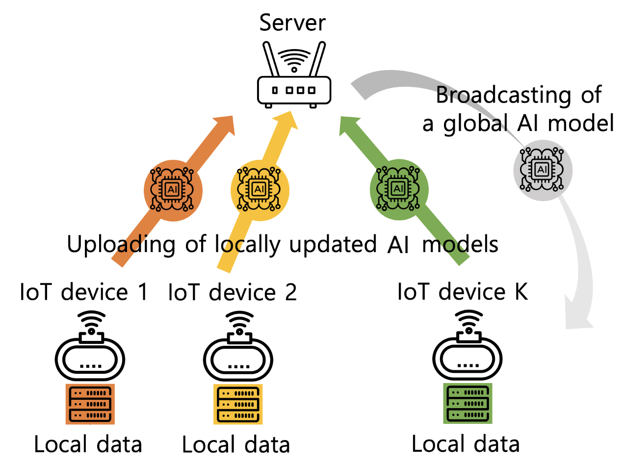
We consider a federated learning system depicted in Fig. 1 consisting of a single server and IoT devices. Each device has its own local data set , where . Then, the entire data set in this system is represented as . The aim of the federated learning system is to find an optimal global model which fits to the entire data set without directly accessing to local data. Specifically, let denote a global model and its global loss function is defined as
| (1) |
where is the local loss function for device measured by the local data set . In other words,
| (2) |
where is the loss function for each data sample . Hence, an optimal model can be expressed as
| (3) |
and the corresponding minimum global loss is given by .
To protect local data stored at the devices, the server is not allowed to directly access to local data stored at the devices. Hence, each device is required to compute and update local model based on its own local data set. After updating, the updated local model will be delivered to the server. The server then receives the updated local models from the devices and aggregates them to produce a global model for the next iteration. By iterating such local update at each device and aggregation at the server, the federated learning system can obtain an optimal global model without accessing local data stored in devices.
Due to the large scale of data stored on devices, we use stochastic gradient descent for updating models. Stochastic gradient descent involves computing gradients with randomly selected data samples. The subset of data samples chosen for computing gradients is called a batch. Thus, if device utilizes batch of size at the th iteration, the stochastic gradient is represented as
| (4) |
where denotes the global model at the th iteration. Without loss of generality, we assume that the batch size is assigned in ascending order with respect to the device index , i.e., if . We assume that the stochastic gradient is an unbiased estimator of the true gradient. In other words,
| (5) |
is satisfied, where the expectation takes with respect to which is a chosen data sample at the th iteration. By using the stochastic gradient in (4), device updates the global model at the th iteration as
| (6) |
where is the step size at the th iteration.
Then, after receiving for all at the server, the global model for the th iteration is constructed as
| (7) |
where . Note that is an updated local model at device and is different from a global model , which is the output of aggregation at the server.
Remark 1
The main focus of this paper is about batch allocation and the corresponding transmission control between devices when the same number of data samples for batches is assumed at each iteration. For notational simplicity, therefore, denote by ignoring the index .
Through the repetition of local updates on devices and global aggregation at the server, an optimal global model can be obtained. In this paper, our focus is on the completion time required to obtain an updated global model at the server, approaching the optimal state within a certain gap. To measure the completion time, we adopt a time-slotted model where each time slot is defined as a specific duration. Consequently, by counting the number of time slots needed to establish the optimal model, we can measure the completion time for federated learning.
II-B Minimization of Completion Time
In this paper, the completion time of the federated learning system is defined as the time duration for constructing that satisfies
| (8) |
where is a target optimality gap. Provided that a model at the th iteration satisfies (8), the completion time is represented as
| (9) |
where is the time duration for updating at the th iteration.
In federated learning, each iteration consists of four steps: 1) distribution of a global model from the sever to each device; 2) local updating at each device based on its own data; 3) transmission of an updated model from each device to the server; 4) aggregation of updated models at the server. For model distribution, the server can broadcast an aggregated model to all devices using a downlink shared channel. Additionally, the computing capability of the server is generally much better than that of IoT devices. Therefore, we focus on steps 2 and 3 to evaluate .
Let represent the required time duration for device at the th iteration. Then. . The aim of this paper is to minimize the expected completion time that is represented as
| (10) |
where the expectation accounts for the randomness of batch constructions and communications depending on transmission protocols.
II-B1 Computing time for local updates
We assume that the computing capability of devices are the same such that each device can compute gradient of data samples per time slot. Recall that the batch size of device at the th iteration is given by . Hence, if we represent the computing time of device at the th iteration as , we have
| (11) |
where is the ceiling function.
II-B2 Communication time for model transmission
Description of transmission protocols of nodes for updated model delivery to the server is more complicated than the computing time description. For simplicity, we assume that each slot duration is normalized such that a single model can be transmitted from a device to the server. However, as multiple devices participate in federated learning, a multiple access protocol between devices is required to send their updated models. In this paper, we consider two fundamental multiple access schemes: TDMA and RA.
In the case of TDMA, a central scheduler can allocate distinct time slots for each of the devices, thereby avoiding interference or collisions that might occur due to simultaneous transmissions from multiple devices. On the other hand, RA allows each device to decide its transmission in a distributed manner, so that collisions can occur. Thus, each device is required to repeatedly transmit its updated model with a certain probability until successful transmission occurs. The detailed analysis on the communication time for both TDMA and RA will be given in Section IV.
III Characterization of the Number of Required Iterations
From the definition in (8), is the expected number of iterations required for constructing a global model that can achieve a minimum global loss within a constant gap of . In this section, we characterize when the target optimality gap is given. To analyze the convergence behavior of the federated learning system, we introduce the following assumptions that hold for arbitrary models and .
Assumption 1
The global loss function is -smooth. Specifically,
| (12) |
for any and .
From Assumption 1, the following inequality holds for any and :
| (13) |
where is the inner product of and .
Assumption 2
The global loss function is -strongly convex. Specifically,
| (14) |
for any and .
Assumption 3
For some constant , the mean squared norm of stochastic gradients are upper-bounded by
| (15) |
for all .
From Assumption 2, the following Lemma holds.
Lemma 1
Suppose that is -strongly convex. Then, for any ,
| (16) |
Proof:
From Assumption 3, we can obtain the following lemma which bounds the second moment of stochastic gradients dependent on the batch size.
Lemma 2
Recall that is the stochastic gradient computed at device in the th iteration with batch size . From Assumption 3, the second moment of is upper-bounded as
| (20) |
for all and .
Proof:
Now, using the given assumptions and lemmas, we can find the number of iterations required to achieve the optimality gap .
Theorem 1
Set the sequence of step sizes as
| (23) |
for some constants , and . Suppose that is the global model at the th iteration. Then
| (24) |
is satisfied, where
| (25) |
Proof:
From the -smoothness in (13),
| (26) |
where the first equality holds from (6) and (7). Then, by taking the expectation with respect to defined as batches chosen at the th iteration by all devices, we have
| (27) |
where the second inequality holds from (5). Here, the expectation is over the distribution of data selected for the th iteration and becomes deterministic at the th iteration.
The second term in (III) is further upper-bounded by
| (28) |
where holds since for all and holds from Lemma 2. Hence, from (III) and (III), we have
| (29) |
where the result in Lemma 1 is used.
By taking the expectation for both sides of (III) over the whole sequence of samples chosen until the th iteration, the following inequality is obtained after some manipulations:
| (30) |
Corollary 1
Given , is satisfied if . That is,
| (33) |
Proof:
IV Analysis on Iteration Time
In Section III, we have characterized the number of required iterations as a function of . To specify the expected completion time in (II-B), the expected time duration required for each iteration should be analyzed. Moreover, as the randomness from data selection and communication is identical to every iteration, the expected iteration time is the same. Thus, to enhance readability and avoid confusion, we omit the iteration index from here on.
As stated in Section II-B, the required time duration for local updates is straightforwardly given as (11). Hence, after , device is available for transmitting its updated local model. We focus on the analysis of communication time for updated model transmission in this section. As briefly mentioned in Section II-B2, this paper explores exemplary communication models of both centralized and distributed, namely TDMA and RA, respectively. In the following two subsections, we investigate the iteration time for each multiple access scheme.
IV-A Iteration Time for TDMA
For TDMA, multiple devices are scheduled to transmit in different time slots. Suppose that, at a certain time slot, only one device has completed its local updates. In such a case, it’s evident that the device should transmit during that time. However, if multiple devices are ready for transmission, without loss of generality, we assume that the server prioritizes scheduling the device with the lower index first. Note that device indices are assigned in ascending order according to the batch size. Consequently, the time slot when device is scheduled to transmit is given as
| (35) |
where is the time slot when device is scheduled to transmit and .
Since the iteration time is defined as the time duration until the last device has delivered its local model to the server, the iteration time is the same as the time slot scheduled for the device which has the largest batch size. Therefore,
| (36) |
where the last equality holds since for any , , and . Then, by applying (35) recursively, the iteration time using TDMA can be rewritten as
| (37) |
IV-B Iteration Time for RA
In the case of RA, we assume a simple RA protocol where each device decides whether to transmit or not using a certain probability known as the transmission probability, denoted by . As a result, multiple devices may transmit during the same time slot, leading to potential collisions. In essence, successful transmission takes place only if one of the devices transmits while the others remain silent. In the event of a collision, retransmission of the updated model becomes necessary until the server successfully receives it. Consequently, the probability of successful transmission when devices are available for transmission is expressed as
| (38) |
As seen in (38), successful transmission is probabilistically determined and, as a consequence, the number of time slots used for delivering updated models is also stochastically given. Hence, we consider the expected iteration time denoted as .
Note that the devices finishing local updates attempt transmission of their updated models to the server. Hence, device , which is allocated the largest batch size, can send updated model after . Moreover, due to collision, some devices which have completed updating earlier than device may fail to deliver their updated models until time slot . Hence, device may compete for channel access with other devices that have not successfully transmitted updated models until time slot . Let us denote as the number of devices that are required to transmit their updated models at time slot . Denote as the communication time duration in which devices have successfully delivered their updated models, which is measured from time slot . Then, the expected iteration time for RA is represented by
| (39) |
As devices are attempting for transmission, can be expressed as a sum of inter-delivery time defined as the time duration between consecutive successful deliveries. Let be the th inter-delivery time, measured by the time duration between the th successful transmission and the th successful transmission. We have
| (40) |
Considering that the devices attempt transmission until being successful, follows the geometric distribution. Provided that devices are available at time slot , is geometrically distributed with a probability . After the first successful transmission, the second inter-delivery time is measured with the number of available devices , which means the probability of successful transmission is changed to . Consequently, the conditional probability mass function (PMF) for the th inter-delivery time given that devices are available at time slot is written as
| (41) |
where Then, we have
| (42) |
where holds from the total probability, holds from (40), holds from (41) and the fact that
| (43) |
Next, we will first investigate the distribution of for and , and then consider arbitrary values of .
IV-B1 Two-devices case
Let us consider the case where . Then, becomes either one or two. First, we derive the probability that . The event means that device has succeeded in transmission before time slot . Hence
| (45) |
Obviously,
| (46) |
IV-B2 Three-devices case
For , can be or . Obviously,
| (48) |
The event implies that one of the devices has succeeded in transmission before time slot . Denote the time slot of the first successful delivery by . Then, depending on the value of , we can derive joint probabilities as follows.
Consider an event . When , the event means that all communication attempts are failed during the time slots . Thus,
| (49) |
On the other hand, if , the first successful delivery should occur when device and device are competing each other. In this case, after the first successful delivery, the remaining device is still attempting to transmit. To have for this case, the remaining device fails in delivery during the time slots between and . Therefore, is expressed as in (50).
| (50) |
| (51) |
When , all communication attempts are failed before time slot . Hence,
| (52) |
By replacing and in (48) with (51) and (52), we have
| (53) |
Using the PMF of expressed in (51), (52) and (IV-B2), we obtain for as in (54).
| (54) |
IV-B3 N-devices case
For a general case with devices, the possible range of values for is given by . In this case, we need to consider instances of the successful delivery time. Furthermore, the joint probability of and varies depending on the range of each successful delivery. Additionally, each sequence of successful deliveries has different probabilities due to the varying number of available devices. As an example, when , there exist distinct cases for . Consequently, addressing the complete PMF of and computing for all involves considering numerous cases. As a result, obtaining a closed-form expression for the PMF of becomes intractable. Instead, we can numerically derive the distribution of for a general -device system using Monte Carlo simulations.
V Optimal Batch Allocation
In Section IV, we have analyzed the iteration time for both TDMA and RA protocols when the set of batch sizes are given. In this section, we focus on an optimal batch allocation of under the constraint that .
V-A Completion Time
From (33) and (37), we can rewrite the completion time in (9) for TDMA in (9) as
| (55) |
For the case of RA, the expected completion time is given by
| (56) |
Because the sum of batch size is a constant, the number of iterations required to achieve a target optimality gap becomes also a constant. Thus, to minimize the completion time or the expected completion time, we need to minimize the iteration time for each iteration procedure, which depends on for both TDMA and RA. To minimize waiting or retransmission time for uploading locally updated models, we propose a batch allocation algorithm called the step-wise batch allocation. The pseudo code of the proposed algorithm is stated in Algorithm 1.
V-B Batch Allocation for TDMA
In the following, we will prove that the output of the step-wise batch allocation achieves the minimum iteration time for TDMA.
To show the optimality of the proposed step-wise batch allocation, we first derive a lower bound on when the total batch size is given.
Proposition 1
Suppose that there exists a positive integer satisfying that . Then the iteration time for TDMA is lower-bounded by
| (57) |
Proof:
We prove this proposition by contradiction. For such purpose, assume that is achievable. From (35), every device should be scheduled no later than . That means
| (58) |
for . Moreover, in federate learning, only the devices that have finished their local updates can participate in transmission. Thus,
| (59) |
Combining (58) and (59), we have
| (60) |
Then, from (11) and (60) , we have
| (61) |
Since , we can find an upper bound on using (61).
| (62) | ||||
| (63) |
However, (63) contradicts to the assumption that . As a consequence, , which completes the proof. ∎
By using Proposition 1, we can prove the optimality of the proposed step-wise batch allocation algorithm, stated in Theorem 2.
Theorem 2
Suppose that there exists a positive integer satisfying that . Then the step-wise batch allocation from Algorithm 1 achieves by setting .
Proof:
First, let us consider the case where . For this case, is given by
| (64) |
for . From (64),
| (65) |
and, as a result, we have
| (66) |
Therefore, each device can be scheduled one time slot earlier than the next device. Consequently, at the th time slot, all devices except for device have completed updating models and transmitted updated models to the server. Moreover, device finishes updating at the th time slot. As a consequence, it is possible for device to send its updated model at the th time slot. That means that the step-wise batch allocation algorithm can achieve for .
For , the resulting batch allocation from Algorithm 1 becomes identical to that for by removing some batch assigned in the later loop. Since reducing the allocated batch size cannot increase the computation or communication time, is still achievable for this case. This completes the proof. ∎
V-C Batch Allocation for RA
When RA is employed for transmitting updated models, the time duration for computation and communication affects the expected iteration time, as demonstrated in (44). If the server assigns equal-size batches to all devices, the time required for local updates is reduced by leveraging parallel computing. However, after updating the models, all devices will simultaneously attempt transmission, leading to longer communication times due to heavy contention. On the other hand, if there are variations in batch sizes allocated to devices, the time slot when the last device with the largest batch size completes its updates can be delayed. However, devices with smaller batch sizes will have opportunities to transmit updated models while other devices are still in the process of updating their models.
Hence, it is crucial to allocate an appropriate batch size to each of devices. By combining (11) and (44), the expected iteration time for RA is approximately given as , where we ignore the ceiling operation in (11). Therefore, we aim to address the following optimization problem to minimize the expected iteration time for RA:
| (67) |
subject to
| (68) |
Denote the solution of the optimization problem P1 by . Note that, in order to solve P1, we need to know the distribution of . In Section IV-B, we established a closed-form expression for the distribution of when and . Based on these results, we derive the optimal batch allocation when in the following theorem.
Proof:
By defining the difference between and as , we have and . Then from (47), the original problem P1 can be rewritten as
| (70) |
For notational convenience, denote the objective function in (70) by . Then, the derivative of is given by
| (71) |
Suppose that for . Then, the completion time increases as increases within the feasible range of . As a result, provides the optimal batch allocation, given by . Note that the condition is rewritten as
| (72) |
Hence, if , then holds for .
On the other hand, if for , the completion time decreases as increases. Hence, provides the optimal batch allocation, given by for this case. In a similar manner, if , holds for .
Lastly, there is a case where neither nor holds for . In that case, the optimal condition corresponds to the point where the derivative is equal to zero. Hence, from the condition , we have
| (73) |
Hence, and . This completes the proof. ∎
For , P1 can be rewritten as (74) subject to
| (75) |
where and . Since the optimization problem P3 is a convex programming problem, we can find an optimal solution using the Karush–Kuhn–Tucker (KKT) conditions [19]. Let us denote the objective function in (74) as and the Lagrangian function as
| (76) |
Then, the corresponding KKT conditions are represented as
| (77) | ||||
| (78) | ||||
| (79) | ||||
| (80) | ||||
| (81) |
| (74) |
For , obtaining a closed-form expression for the PMF of is intractable since it requires accounting for all combinations of realizations of successful delivery times. However, the optimal solutions for and demonstrate that different sizes of batches between the devices is necessary to reduce the expected iteration time. Moreover, when TDMA is used, the step-wise batch allocation in Algorithm 1 with is shown to be optimal. Hence, for we numerically optimize in Algorithm 1 to minimize the iteration time for RA in Section VI. Unlike TDMA in which a single time slot is required for transmitting the updated model of each device due to centralized scheduling, devices communicate stochastically for RA, which might necessitate a larger number of time slots, i.e., .
VI Experiments
In this section, we present experimental results demonstrating the completion time using real datasets.
We evaluate the performance of the step-wise batch allocation in Algorithm 1 based on the MNIST classification. For the sake of simplicity, we concentrate on binary classification, using only the “” and “” classes from the MNIST dataset, as detailed in [20]. Additionally, we employ the cross-entropy loss function. For this case, we have and . The remaining parameters are set as , , , and .
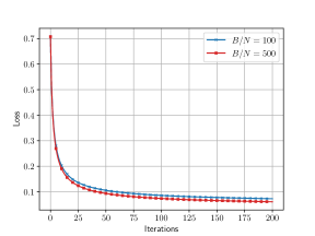
To validate the efficacy of derived in Theorem 1 and Corollary 1, we assess the training loss in Fig. 2. The model undergoes training with an average batch size per device denoted as over a span of 200 iterations. From Corollary 1, the values of and are specified as and respectively for both cases. Notably, at the th iteration, the corresponding loss values are recorded as and for , respectively. Treating the loss value at the 200th iteration as an approximation of the minimum loss, the optimal gap is attained at the th iteration for both cases, while is achieved at the rd iteration for and at the nd iteration for , respectively.
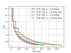
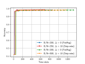
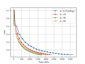
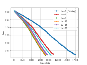
In Fig. 3 and 4, we compare the performance of federated learning with different size of batch gap under the TDMA protocol. We applied the step-wise batch allocation in Algorithm 1. It is worth highlighting that federated learning with is essentially equivalent to FedAvg [2]. As seen in the figures, the step-wise batch allocation with exhibits faster convergence compared to FedAvg, which corresponds to the case where . Indeed, Theorem 2 proved that the proposed step-wise batch allocation with minimizes the completion time.
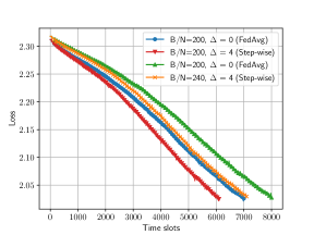
In Fig. 5, we evaluate the value of loss function as a function of time slots using RA for , , and . We again applied the step-wise batch allocation in Algorithm 1. Although the communication protocol has been changed from TDMA to RA, models are updated and aggregated under the same rule using SGD. Consequently, performance of learning does not change notably even after change of communication protocol. As seen in the figure, the step-wise batch allocation with shows fastest reduction of loss function compared with the case where .
For , the optimal batch allocation was determined in Theorem 3 by disregarding the ceiling operation. In Fig. 6, the gap between iteration time and average computing time, defined as , is compared with experimental results. In the figure, ‘Opt. with integer relaxation’ corresponds to the solution of (70). Then, ‘Opt. without integer relaxation’ is obtained by applying the ceiling operation to ‘Opt. with integer relaxation’. Due to integer constraints, a gap from the theoretically optimal point obtained under integer relaxation is inevitable. However, this gap can be considered negligible.
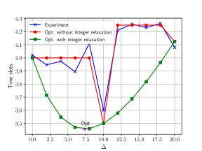
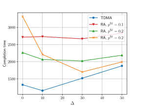
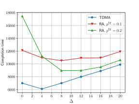
Fig. 7 represents the completion time as a function of for different values of the transmission probability for RA. The completion time of TDMA is also included. When TDMA is utilized, the server schedules transmissions in a way that avoids collisions, resulting in the lowest completion time for federated learning. Moreover, as for RA increases, the performance of step-wise batch allocation with an appropriate batch gap achieves a lower completion time. It is known that the that minimizes communication time for RA is given as the inverse of the number of nodes [21]. Thus, for , the optimal transmission probability is determined as . However, when comparing the completion times for and in Fig. 7, the completion time for is smaller than that of by properly setting .
In addition to the MNIST dataset, we conducted experiments with the CIFAR-10 dataset. For CIFAR-10 classification, we employed a convolutional neural network (CNN). Since CNN does not adhere to the assumptions that allow us to determine the required number of iterations, we set the number of iterations to for training CNN. With , , and , we present the results for the loss function using TDMA and RA, and the completion time in Figs. 8, 9, and 10, respectively. We consider the batch gap size in the set .
As observed in the figures, the step-wise batch allocation in Algorithm 1 significantly reduces the completion time without compromising the model’s performance. In particular, the optimal batch gap is given by for TDMA, i.e., in Theorem 2. The minimum completion time is achievable when for RA. Note that the values of the optimal batch gap in Fig. 10 are smaller than those in Fig. 7. This is because the computing capability of each node is reduced from to , making a smaller size of the batch gap sufficient to cause a deviation in computing time across devices. For instance, a batch gap larger than results in unnecessary idle time slots, leading to a longer completion time.
VII Conclusion
In this paper, we thoroughly investigated completion time, representing the time required for federated learning over a wireless channel to achieve a predefined performance for a machine learning model. In our pursuit of characterizing completion time, we derived the number of iterations necessary to reach the desired performance level and analyzed the time duration for each iteration.
In scenarios where the server can allocate time slots for communication with each device, we introduced a novel batch allocation algorithm. Our research has conclusively demonstrated the optimality of this proposed algorithm in minimizing completion time. Moreover, when random access is employed, the use of identical batch sizes results in a high number of packet collisions, leading to extended duration for each iteration. To address this issue and further reduce completion time, we introduced a batch allocation algorithm that leverages batch gaps between devices. By allowing different batch sizes for each device, we successfully mitigated contention for channel access. As a result, the step-wise batch allocation approach, incorporating suitable batch gaps while considering factors such as batch size, computing speed, and transmission probability, emerges as a promising strategy for reducing completion time.
Our findings underscore the importance of optimizing wireless federated learning systems from a holistic perspective that encompasses both communication and computation aspects. The synergy between these two domains is crucial for achieving efficient and effective federated learning over wireless networks.
References
- [1] Ericsson, “Ericsson mobility report,” 2023. [Online]. Available: https://www.ericsson.com/en/reports-and-papers/mobility-report/reports/june-2023
- [2] B. McMahan, E. Moore, D. Ramage, S. Hampson, and B. A. y Arcas, “Communication-efficient learning of deep networks from decentralized data,” in Proc. of the 20th International Conference on Artificial Intelligence and Statistics, Apr. 2017, pp. 1273–1282.
- [3] P. Kairouz, H. B. McMahan, B. Avent, A. Bellet, M. Bennis, A. N. Bhagoji, K. Bonawitz, Z. Charles, G. Cormode, R. Cummings et al., “Advances and open problems in federated learning,” Foundations and Trends® in Machine Learning, vol. 14, no. 1–2, pp. 1–210, 2021.
- [4] T. Zhang, L. Gao, C. He, M. Zhang, B. Krishnamachari, and A. S. Avestimehr, “Federated learning for the internet of things: Applications, challenges, and opportunities,” IEEE Internet of Things Magazine, vol. 5, no. 1, pp. 24–29, 2022.
- [5] J. Konečnỳ, H. B. McMahan, F. X. Yu, P. Richtárik, A. T. Suresh, and D. Bacon, “Federated learning: Strategies for improving communication efficiency,” arXiv preprint arXiv:1610.05492, 2016. [Online]. Available: https://arxiv.org/abs/1610.05492
- [6] S. U. Stich, “Local sgd converges fast and communicates little,” arXiv preprint arXiv:1805.09767, 2018.
- [7] H. Yu, S. Yang, and S. Zhu, “Parallel restarted sgd with faster convergence and less communication: Demystifying why model averaging works for deep learning,” in Proceedings of the AAAI Conference on Artificial Intelligence, vol. 33, no. 01, 2019, pp. 5693–5700.
- [8] G. Lan, S. Lee, and Y. Zhou, “Communication-efficient algorithms for decentralized and stochastic optimization,” Mathematical Programming, vol. 180, no. 1-2, pp. 237–284, 2020.
- [9] C. Liu, H. Li, Y. Shi, and D. Xu, “Distributed event-triggered gradient method for constrained convex minimization,” IEEE Transactions on Automatic Control, vol. 65, no. 2, pp. 778–785, 2019.
- [10] L. Gao, S. Deng, H. Li, and C. Li, “An event-triggered approach for gradient tracking in consensus-based distributed optimization,” IEEE Transactions on Network Science and Engineering, vol. 9, no. 2, pp. 510–523, 2022.
- [11] Z. Yang, M. Chen, W. Saad, C. S. Hong, and M. Shikh-Bahaei, “Energy efficient federated learning over wireless communication networks,” IEEE Transactions on Wireless Communications, vol. 20, no. 3, pp. 1935–1949, 2020.
- [12] X. Cao, G. Zhu, J. Xu, Z. Wang, and S. Cui, “Optimized power control design for over-the-air federated edge learning,” IEEE Journal on Selected Areas in Communications, vol. 40, no. 1, pp. 342–358, 2022.
- [13] M. Chen, H. V. Poor, W. Saad, and S. Cui, “Convergence time optimization for federated learning over wireless networks,” IEEE Transactions on Wireless Communications, vol. 20, no. 4, pp. 2457–2471, 2020.
- [14] S. Wan, J. Lu, P. Fan, Y. Shao, C. Peng, and K. B. Letaief, “Convergence analysis and system design for federated learning over wireless networks,” IEEE Journal on Selected Areas in Communications, vol. 39, no. 12, pp. 3622–3639, 2021.
- [15] J. Song and M. Kountouris, “Wireless distributed edge learning: How many edge devices do we need?” IEEE Journal on Selected Areas in Communications, vol. 39, no. 7, pp. 2120–2134, 2020.
- [16] A. Devarakonda, M. Naumov, and M. Garland, “Adabatch: Adaptive batch sizes for training deep neural networks,” arXiv preprint arXiv:1712.02029, 2017.
- [17] J. Zhang, S. Guo, Z. Qu, D. Zeng, Y. Zhan, Q. Liu, and R. Akerkar, “Adaptive federated learning on non-iid data with resource constraint,” IEEE Transactions on Computers, vol. 71, no. 7, pp. 1655–1667, 2022.
- [18] D. Shi, L. Li, M. Wu, M. Shu, R. Yu, M. Pan, and Z. Han, “To talk or to work: Dynamic batch sizes assisted time efficient federated learning over future mobile edge devices,” IEEE Transactions on Wireless Communications, vol. 21, no. 12, pp. 11 038–11 050, 2022.
- [19] S. Boyd and L. Vandenberghe, Convex optimization. Cambridge university press, 2004.
- [20] Y. Shi, Y. Zhou, and Y. Shi, “Over-the-air decentralized federated learning,” in 2021 IEEE International Symposium on Information Theory (ISIT), 2021, pp. 455–460.
- [21] S.-W. Jeon and H. Jin, “Online estimation and adaptation for random access with successive interference cancellation,” IEEE Transactions on Mobile Computing, vol. 22, no. 9, pp. 5418–5433, 2023.