Performance Analysis and ISI Mitigation with Imperfect Transmitter in Molecular Communication
Abstract
In molecular communication (MC), molecules are released from the transmitter to convey information. This paper considers a realistic molecule shift keying (MoSK) scenario with two species of molecule in two reservoirs, where the molecules are harvested from the environment and placed into different reservoirs, which are purified by exchanging molecules between the reservoirs. This process consumes energy, and for a reasonable energy cost, the reservoirs cannot be pure; thus, our MoSK transmitter is imperfect, releasing mixtures of both molecules for every symbol, resulting in inter-symbol interference (ISI). To mitigate ISI, the properties of the receiver are analyzed and a detection method based on the ratio of different molecules is proposed. Theoretical and simulation results are provided, showing that with the increase of energy cost, the system achieves better performance. The good performance of the proposed detection scheme is also demonstrated.
Molecular communication (MC), imperfect transmitter, energy cost, inter symbol interference (ISI).
1 Introduction
Molecular communication (MC), which is inspired by biological communication, employs molecules as information carriers between nanomachines [1, 2, 3]. MC is envisioned as a promising approach to the problem of communication in nanoscale networks [4]. MC has various potential healthcare applications in health monitoring, disease diagnosis, and targeted drug delivery[5]. MC has also been employed to model the spread of infectious disease via aerosols during the outbreak of COVID-19 [6, 7, 8].
In MC, as the molecules released from the transmitter diffuse freely to the receiver without external energy, diffusion-based molecular communication (DMC) is highly energy efficient in terms of propagation. However, due to the small size of the nanomachine, its energy reserves are restricted. Therefore, energy efficiency becomes a significant constraint in DMC, so energy cost in DMC can not be ignored, especially in creating the transmitter. Related works in the literature have considered transmitter design in terms of molecule synthesis: for example, an energy model for DMC considering the energy expended on molecule synthesis, secretory vesicle production, and vesicle transportation to the cell membrane is proposed in [9]. In [10], thermodynamic energy consumption associated with particle emission in DMC signal transmission is studied. In [11], from the thermodynamic properties, the energy cost of DMC is studied without considering the diffusion of the molecules. To improve the energy efficiency, in [12], a power adjustment technique and a decision feedback filter are proposed. In [13], a DMC powered by a nanoscale energy-harvesting mechanism is studied.
In MC, the transmitter can either generate signaling molecules as needed or have a reservoir of such molecules available for transmission [2, 14]. In this paper, we focus on the latter case, where signaling molecules are stored in a reservoir, and harvested from the environment [15]. Even if molecules are synthesized as needed [9, 16], for example by genetically engineered bacteria [17], it is still necessary to store them at least briefly. Furthermore, the molecules in these reservoirs are not necessarily pure: in addition to the intended molecules, there also exist interfering molecules. In biological systems, it is common for cells or tissues to release information molecules that also contain other types of molecules. A specific example of such a phenomenon can be observed with Antimicrobial Peptides (AMPs). AMPs are a class of small molecular proteins that exhibit antimicrobial activity and contribute to immune defense [18, 19]. In certain cases, a single cell has the capability to release two types of AMPs. Some AMPs act as signaling molecules, influencing the behavior of other cells and modulating immune responses. On the other hand, there are AMPs that function as interfering molecules, targeting and disrupting the physiological processes of pathogens. This interference can occur through various mechanisms such as the disruption of pathogen cell membranes, interference with their metabolism, or inhibition of their growth [20].
In MC, information is encoded in the physical properties of the molecules (e.g. the number of molecules, the type of molecules, or the release time of the molecules). In this paper we use the type of molecules to encode information, a method known as molecule shift keying (MoSK). For example, in binary molecular shift keying (BMoSK), two types of molecules are required to encode the information: bit 0 is expressed with molecule A, while bit 1 is expressed with molecule B; the receiver can then decide which bit was sent based on whether it observes more of one molecule than the other. Variants of MoSK are actively studied. A depleted MoSK scheme is proposed in [21], where multiple types of molecules are simultaneously employed to transmit the parallel streams of concentration shift keying for each symbol. In [22], a molecular transition shift keying scheme is proposed, in which two types of molecules can be released, but the released molecule type is chosen based on previous transmissions. In [23], the performance of DMC systems with BMoSK modulation was analyzed. In [24], a layered molecular shift keying (LMoSK) modulation scheme was proposed in which each type of molecule was used to define a communication layer.
In MC, diffusion results in channel memory and inter-symbol interference (ISI), which reduce the information rate [12]. To mitigate these issues, modulation/channel coding schemes [25, 26, 27, 28, 29] and detection schemes [30, 31, 32, 33, 34, 35, 36, 37] have been proposed. Arjmandi et al. [25] proposed an ISI-avoiding modulation scheme by enlarging the time instances of the same type of molecules. In [28], molecular type permutation shift keying was proposed, which mitigates ISI by encoding the information bits in permutations of diverse types of molecules. A precoder scheme based on the concentration difference of two types of molecules was also proposed to mitigate the ISI. In [29], a hybrid modulation scheme was proposed to mitigate ISI based on molecules pulse position and concentration. In [38], a binary direction shift keying modulation scheme is proposed to mitigate multiuser interference, wherein molecules are released in two different directions. By studying the local convexity of the received signals, Li et al. [30] proposed to detect the received symbols based on molecular concentration difference. Chang et al. [31] proposed an adaptive detection scheme to mitigate ISI based on the reconstruction of the channel impulse response. Maximum likelihood (ML) detection schemes [32, 33, 34] and symbol-by-symbol ML detection schemes [35, 36] have also been proposed in molecular communication. Moreover, non-coherent detection schemes based on K-means clustering were studied in [37]. Further machine learning methods have been proposed to mitigate the ISI in molecular communication [39, 40]. However, for machine learning schemes, it is challenging to obtain substantial amounts of data for training.
In this paper, based on the works from [11], which investigated the purification process involving the movement of molecules between reservoirs, it was revealed that the establishment of reservoirs incurs a free energy cost. However, due to practical energy constraints, achieving complete separation of different molecule types becomes infeasible; as a result, it is necessary to tolerate partially impure reservoirs. This impurity, in turn, causes significant interference at the receiver. Consequently, we address an MC system with an imperfect transmitter featuring two reservoirs. Within these reservoirs, molecules are mixed, and distinctions between the two molecule types are created by moving molecules between the reservoirs. This transfer process necessitates energy input, and due to practical energy considerations, the reservoirs contain interfering molecules, which leads to severe interference at the receiver. Unlike [41] where the errors in an imperfect transmitter arise from the molecules being probabilistically released from the transmitter membrane, and unlike [11], which primarily centers on the energy consumption associated with moving molecules between reservoirs, this paper provides an analysis of system performance in the presence of an imperfect transmitter, ISI, and counting noise. Additionally, a detection method is proposed to mitigate ISI based on the ratio of different molecules.
The main contributions of this paper are summarized as follows.
-
•
An imperfect transmitter is considered, where one kind of molecule is moved from one reservoir to the other and the energy consumption is analyzed.
-
•
As the released molecules contain interfering molecules, we analyze the properties of the received molecules under the imperfect transmitter and the channel memory.
-
•
A detection method based on the ratio of different types of molecules is proposed to mitigate the ISI.
The remainder of this paper is organized as follows. In section II, we introduce the system model of the considered imperfect transmitter MC system. In section III, the performance of the proposed imperfect transmitter MC system is analyzed. Numerical and simulation results are presented in Section IV. Finally, in Section V, we conclude this paper.
2 System Model
Consider a system, analogous to the one described in [11], wherein the environment comprises a mixture of two molecular types, denoted as and . In this context, we make the assumption that and exclusively constitute the molecular composition of the environment. The initial concentration of these molecules is quantified by a molar fraction of , denoted as . This molar fraction, a metric expressing the concentration of relative to the overall concentration of both and , is defined as the ratio of the moles of to the total moles of both and molecules present in the environment.
In the binary MoSK molecular communication system, two molecular reservoirs are required to store two types of molecules. In this paper, we assume the information molecules collected from the environment are mixed, i.e., each reservoir can contain both kinds of molecules, though at different concentrations. Initially, the contents of the reservoirs are acquired from the environment, resulting in equal concentrations of each type of molecule in the low and high reservoirs. In order to use MoSK, we need a different concentration in each reservoir, so that one primarily contains one molecule and the other primarily contains the other, although in this scenario the concentrations will be impure. Thus, we propose moving one molecular type from one reservoir to the other. This creates a concentration difference between the two reservoirs, allowing the detector to decode information based on the ratio of the two molecular concentrations. However, it is important to note that the act of purifying the reservoirs requires energy. This process increases the chemical potential of the reservoirs with respect to the environment and requires an investment of free energy [42]. Thus, even though no energy is required to synthesize molecules, the thermodynamic properties of the system require a fundamental amount of energy in order to purify the reservoirs.
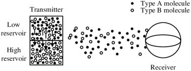
The transmitter creates two reservoirs of molecules from the environmental mixture, both initially at concentration . From these, it creates a difference of concentration between the two reservoirs by transferring molecules of from one to the other: the donating reservoir is called the low reservoir, with concentration ; while the receiving reservoir is called the high reservoir, with concentration . (The terms low and high refer to the concentration of , which is low in the donating reservoir and high in the receiving reservoir.) However, due to practical energy constraints during the moving process, complete separation of different molecule types becomes infeasible. This results in reservoirs containing interfering molecules that are subsequently released, contributing to the occurrence of severe ISI at the receiver. The transmitter sends a bit by selecting molecules from either the low reservoir (to send 0) or the high reservoir (to send 1). The communication system is depicted in Figure 1. The reservoirs are replenished at the beginning of the communication session and contain a sufficient number of molecules in order to transmit all required symbols. To create the concentration difference of A and B molecules between the low and high reservoirs, B molecules are moved from the low reservoir to the high reservoir, a process which consumes free energy. The ratio in each reservoir is not actively controlled, but the method of selecting molecules for transmission will maintain the concentration constant, on average, in each reservoir.
Creating the reservoir requires an input of free energy because of the changing chemical potential. From [11], if molecules of type are moved from the low reservoir to the high reservoir (where is small compared to the total number of molecules in the reservoir), then the energy cost can be expressed as [11, Eqn. (25)]
| (1) |
where and are the total number of molecules in the low and high reservoirs, respectively, is Boltzmann’s constant, is the absolute temperature, and are the fraction of molecules in the low and high reservoirs, respectively. Then, after moving molecules of type from the low reservoir to the high reservoir, the mole fractions of type molecules in the low and high reservoirs can be approximated as
| (2) | ||||
To analyze the performance of our transmission scheme, from (1), we focus on how the number of moved molecules varies with the energy . Assume that , and let represent the total number of molecules in both reservoirs. Then (1) can be expressed as
| (3) | ||||
To simplify the notation, define , the number of molecules moved as a fraction of the reservoir size, and define . Then (3) can be expressed as
| (4) |
By assumption, the number of moved molecules is much smaller than the number of molecules in the low or high reservoir. Thus, . By employing a Taylor series [43, 44], we can write
| (5) | ||||
Therefore, (4) can be expressed as
| (6) | ||||
From now on we will ignore the term. Therefore, for the given energy cost, the number of moved molecules can be expressed as
| (7) |
Then, based on (2), and can be expressed as
| (8) | ||||
The number of and molecules in the low and high reservoirs are respectively
| (9) | ||||
After moving molecules of type from the low reservoir to the high reservoir, there is a concentration difference of molecules between the low and high reservoir, and can be expressed as , where and are the concentration of and molecules in the low reservoir, and are the concentration of and molecules in the high reservoir, respectively. In the communication process, MoSK is employed. Therefore, during the th bit interval, to transmit molecules from the low reservoir for bit , the transmitted signal can be expressed as
| (10) |
where is a random variable representing the fraction of selected molecules of each type, i.e., is the fraction of molecules in the selected molecules (where the mean fraction of molecules in the low reservoir is , which is the transmitted signal); and is the fraction of molecules in the selected molecules (where the mean fraction of molecules in the low reservoir is , which is interference).
Similarly, to transmit molecules from the high reservoir for bit , the transmitted signal can be expressed:
| (11) |
where is the fraction of molecules in the selected molecules and the mean fraction of molecules in the high reservoir is , which is interference; is the fraction of molecules in the selected molecules and the mean fraction of molecules in the high reservoir is , which is intend to transmit.
3 Performance analysis
Our goal in this paper is to find a tradeoff between the chemical potential energy required to create the transmitter, and the bit error rate from using the transmitter; thus, in this section, we derive an expression for the probability of error. Compared to the traditional MoSK, the performance analysis in the considered MC system with an imperfect transmitter is more challenging, as the transmitted molecules are mixed with and molecules whether for bit 0 and bit 1. Meanwhile, as the released molecules include the intended molecules and the other type of molecules, which are interference molecules, therefore, the released mixed molecules make more severe ISI compared to the traditional MoSK in MC, resulting in the BER performance decrease. In this section, we focus on the analysis of the system performance of the considered MC system with the imperfect transmitter. Assuming the probability of transmitting bit 0 is , so the probability of transmitting bit 1 is .
3.1 Analysis of the received molecules
Compared to the distance between the transmitter and the receiver, the size of the information molecules and reservoirs are assumed to be very small, then, the transmitter is modeled by a point transmitter. Considering a 3D absorbing receiver, the fraction of molecules absorbed by the receiver until time , , can be expressed as
| (12) |
where is the radius of the receiver, is the distance between the transmitter and the receiver, is the diffusion coefficient of the released molecules (The diffusion coefficient of and molecules are assumed to be the same, which is a common assumption in MC, such as for isomers [45]). Considering molecules are released by the transmitter and the transmitted signal, the the average number of received molecules can be expressed as
| (13) |
During the th bit interval, the hitting probability can be expressed as
| (14) |
where is the bit interval.
As the transmission contains and molecules, the mean number of received molecules can be expressed as
| (15) |
where is the number of received molecules during the th bit interval which molecules transmitted at the beginning of th bit interval, is the number of molecules received during the th bit interval but transmitted from the previous bit interval and defined as ISI, is the counting noise of molecules which can be modeled by the Gaussian distribution , where depends on the average number of received molecules. The quantity can be expressed as
| (16) |
where is the transmitted molecules in the th bit interval and selected from the low or high reservoir; is the fraction of molecules in the selected reservoir; is the probability of molecules transmitted at the beginning of the th bit interval and observed by the receiver during the th bit interval.
The number of molecules received as ISI, , can be expressed as
| (17) |
where is the number of ISI molecules which are transmitted at the th bit interval and can be expressed as
| (18) |
where is the probability of molecules transmitted at the beginning of th bit interval and observed by the receiver during the th bit interval. As the number of transmitted molecules is large, then, can be approximated by a normal distribution: . Therefore, can also be approximate by a normal distribution.
Similarly, the mean number of received molecules can be expressed as
| (19) |
where
| (20) |
| (21) |
and can be expressed as
| (22) |
Similarly, can be approximated by a normal distribution: . Therefore, can also be approximate by a normal distribution. is the counting noise of molecules which can be modeled by the Gaussian distribution , where depends on the average number of received molecules.
3.2 Detection and ISI mitigation
The detector can be formulated by the binary hypothesis testing problem with the received and molecules. Though in [46], a binary hypothesis testing scheme has been employed, however, different to [46], in this paper, due to the imperfect transmitter, the transmitted molecules are mixed, making the analysis of received molecules more complex. The hypotheses are given by:
-
•
: molecules are emitted from the low reservoir. ;,
-
•
: molecules are emitted from the high reservoir; ;;
where and denote the probability density function of received and molecules under , respectively, while and denote the probability density function of received and molecules under , respectively. As the and molecules select from the low or high reservoir by probability and the number of transmitted molecules is large, therefore, and can be approximated by the normal distribution [9].
Under hypothesis , the mean number of received and molecules can be expressed as
| (23) |
and
| (24) |
where and are the fraction of and molecules in the selected reservoir, respectively. And the number of received and molecules under can be approximated by the normal distribution, , . The mean and variance of received molecules under during the th bit interval can be expressed as
| (25) | ||||
and as the symbols are selected independently and propagation of each molecule is independent, the event that a molecule arrives at the receiver in a particular interval is independent of every other molecule, thus, the sum of these events as in equation ( 25) is also independent, so the variance of the sum is the sum of the underlying variances.
| (26) | ||||
where
| (27) | ||||
The mean and variance of received molecules under during the th bit interval can be expressed as
| (28) | ||||
and
| (29) | ||||
where
| (30) | ||||
While under hypothesis , the mean number of received and molecules can be expressed as
| (31) | ||||
and
| (32) | ||||
Therefore, the number of received and molecules under follows can be approximated by the normal distribution, , . The mean and variance of received molecules under during the th bit interval can be expressed as
| (33) | ||||
and
| (34) | ||||
where is given by (27). The mean and variance of received molecules under can be expressed as
| (35) | ||||
and
| (36) | ||||
where is given by (30).
Since the transmitted molecules comprise a mixture of type and type molecules, and the ratio of A to B differs between the low and high reservoirs. Therefore, at the receiver, based on the Neyman-Pearson criterion, the maximum likelihood decision rule in the th bit interval can be expressed as
| (37) | ||||
where denotes the ratio of received A and B molecules under , denotes the ratio of received A and B molecules under , and is the decision threshold. Therefore, at the receiver, we can employ to determine the received bits, and the decision rule can be expressed as
| (40) |
Based on (23) (30), under , , where and . Based on (31) (36), under , , where and . Therefore, and .
Obviously, the proposed detector effectively reduces the influence of interference molecules, consequently mitigating ISI. Furthermore, as the energy cost increases, the gap of molecules between the low and high reservoir widens. This reduction in released interference molecules leads to a more pronounced mitigation of ISI.
The average probability of error () from time slot 1 to can be expressed as [47]
| (41) |
The detailed calculation of is shown in the appendix.
4 performance evaluation
In this section, we analyze the performance of the considered MC system with an imperfect transmitter. In the simulation, the parameters are set in Table I. Especially, the Particle-Based Simulator (PBS) for MC is a simulation framework designed to emulate the behavior of individual molecules. In this simulation, the bit interval is discretized into time steps of duration . Each step involves the movement of molecules, and their movement in each direction follows a Gaussian distribution with a mean of 0 and a standard deviation of , where is the diffusion coefficient of information molecules. Notably, the Signal-to-Noise Ratio (SNR), representing the ratio of the average squared number of observed molecules to the noise power[48], is set at 15dB.
| Symbol | Explanation | Value |
|---|---|---|
| Diffusion coefficient | m2/s | |
| Distance between transmitter and receiver | 10 m | |
| Radius of the receiver | 4 m | |
| Bit interval | 1 s | |
| Discrete steps | 100 | |
| Number of transmitted molecules | 1000 | |
| Boltzmann’s constant | 1.3807 | |
| Absolute temperature | 298.15 |
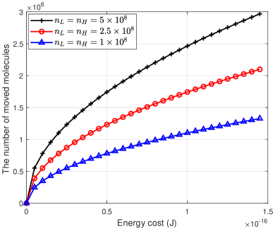
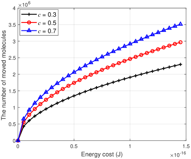
In Figs. 2 and 3, the number of molecules moved between reservoirs is shown to vary with the energy cost, measured in Joule (J), for different numbers of molecules in the reservoirs, as derived in (7). The number of moved molecules increases with the energy cost, and for the given energy cost, for more molecules (as shown in Fig. 2) or higher concentration of molecules in the reservoirs (as shown in Fig. 3), a larger number of molecules can be moved. With the increase of moved molecules, the lower concentration of molecules in the reservoir, then, the larger energy cost is required. These results illustrate that creating a near-perfect transmitter (where each reservoir contains only one kind of molecule) is very costly.
In Fig. 4, we analyze how the BER varies with detection threshold under different mole fractions of molecules in the low and high reservoirs, as derived in (41). It is shown in Fig. 4 that, for a given mole fraction of molecules in the transmitter, there exists an optimal detection threshold, which varies with the mole fractions of the transmitter. The system achieves better performance for the larger difference of the mole fraction between the low and high reservoirs. In the figure, the “perfect” line indicates the perfect transmitter which means that there are only molecules in the low reservoir and only molecules in the high reservoir, as there is no interference molecule from the transmitter; therefore, it achieves the best performance. Thus, the figure indicates that the system performance can be improved at the cost of energy consumption. As shown in Fig. 8, compared to and , and achieves lower BER, as the ratio of and is larger than and , which results in a more substantial gap in the number of received molecules between A and B. Consequently, when employing the proposed detection scheme, and achieves better BER performance. Moreover, PBS is conducted to validate the analytical results.
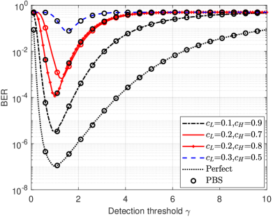
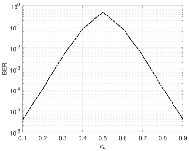
Fig. 5 shows how the BER varies with , which is defined as the mole fraction of molecules in the low reservoir, as derived from (25)-(36) and (39). Recalling the transmission scheme for transmitting each symbol, it can be seen from Fig. 5, when is farther from 0.5, the performance of the system is better; this is because when is farther from 0.5, the fraction of signal molecules is much larger than the interfering molecules. This result also reflects the result in Fig. 4.
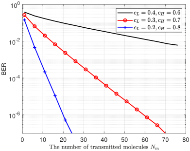
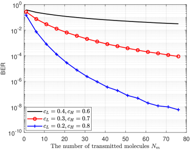
Figs. 6 and 7 demonstrate how the BER varies with the number of transmitted molecules , and clearly show that the BER decreases with the increase of . In Fig. 6, neither ISI nor counting noise are considered, while in Fig. 7, only ISI is considered. Thus, in Fig. 6, BER arises only from the imperfections in the transmitter. Therefore, as the number of transmitted molecules increases, the error probability of selected molecules from the reservoirs decreases. Furthermore, with a larger gap between the and , the concentration of molecules in the low reservoir and the concentration of molecules in the high reservoir are both larger; thus, the BER decreases as the error probability of molecules transmitted from the reservoirs is lower. Meanwhile, in Fig. 7, as counting noise is considered which is related to the number of received molecules and the volume of the receiver, therefore, the slope of the BER decreases with the increase of .
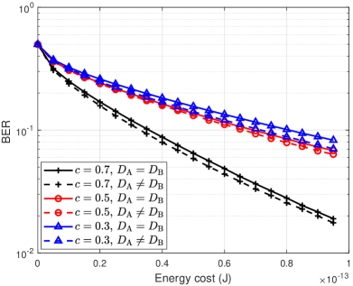
In Fig. 8, we show how the BER varies with the energy cost under differing initial concentrations of molecules in the reservoirs both considering ISI and counting noise as derived from (25)-(36) and (39). As shown in Fig. 8, the BER decreases with the increase of energy cost, as with the increase of energy cost, more molecules are moved from the low reservoir to the high reservoir, then the gap of molecules between the low and high reservoir is larger, therefore, the BER decreases. And due to a reduction in released interference molecules, the ISI can also be mitigated, albeit at the expense of an increased energy cost. For the larger , under the given energy cost, more molecules are moved, and the gap is also larger compared to a small , therefore, it achieves better BER performance. Fig. 8 also indicates that the slope of the BER decreases with the increase of energy cost, indicating a problem of diminishing returns. As shown in Fig. 8, for different diffusion coefficients, the system achieves better BER performance, which is due to one diffusion coefficient being significantly larger: in this case, the released molecules more quickly diffuse away, resulting in less ISI, and better BER performance.
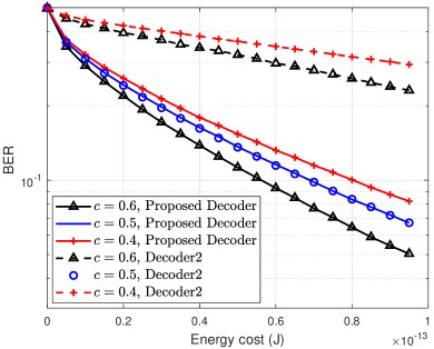
In Fig. 9, we compare the BER performance between the proposed detection method, which is derived in (37), and the conventional detection method (Decoder2), which compares the number of received different types of molecules. As shown in Fig. 9, when , the two decoders achieve the same performance. This is because, when , i.e. there are the same number of A and B molecules initially in the reservoirs, then after moving B molecules from the low reservoir to the high reservoir, there are more A molecules in the low reservoir and more B molecules in the high reservoir; therefore, the same performance is achieved, as seen in the figure. However, when , after moving B molecules from the low reservoir to the high reservoir, it may no longer be the case that there are more A molecules in the low reservoir and more B molecules in the high reservoir, e.g. when , for constant energy cost, after moving B molecules, maybe there are still more B molecules both in the low and high reservoir, making the BER performance of Decoder2 decrease. Therefore, the proposed detector can effectively reduce the impact of interference molecules, simultaneously mitigating ISI.
5 conclusion
In this paper, a molecular communication system with an imperfect transmitter is considered, in which the transmitter contains reservoirs with different concentrations of message-bearing molecules. Unlike the conventional assumption of a perfect transmitter, the molecules in the reservoirs are mixed, but there is a difference between the concentration of different types of molecules. Moreover, our system explicitly takes into account the chemical potential energy required to create the transmitter. Under these assumptions, a detection method based on the ratio of different types of molecules is proposed, and the average BER is derived. Simulation results showed that, with the increase of the difference of concentrations, the system achieves better BER performance, and the ideal transmitter achieves the best performance. However, there is a tradeoff between increased performance and energy expenditure, and we are able to quantify that tradeoff. The imperfect transmitter can also be applied to CSK modulation with a single reservoir, potentially offering a simpler alternative by adjusting the number of molecules that are emitted and mixed with those molecules outside of the reservoir, which would be an interesting topic of future research.
Appendix A
Here we give a detailed calculation of in . This can be detailed expressed as
| (42) | ||||
Assuming , then can be expressed as
| (43) | ||||
The quantity can be expressed as
| (44) | ||||
The quantity can be expressed as
| (45) | ||||
The quantity can be expressed as
| (46) | ||||
The quantities and can be expressed as
| (47) | ||||
| (48) | ||||
| (49) | ||||
| (50) | ||||
where
| (51) | ||||
| (52) | ||||
The variance of the counting noise of type molecules can be expressed as
| (53) | ||||
The variance of the counting noise of type molecules can be expressed as
| (54) | ||||
References
- [1] T. Nakano, A. W. Eckford, and T. Haraguchi, Molecular communication. Cambridge University Press, 2013.
- [2] N. Farsad, H. B. Yilmaz, A. Eckford, C.-B. Chae, and W. Guo, “A comprehensive survey of recent advancements in molecular communication,” IEEE Communications Surveys & Tutorials, vol. 18, no. 3, pp. 1887–1919, 2016.
- [3] V. Jamali, A. Ahmadzadeh, W. Wicke, A. Noel, and R. Schober, “Channel modeling for diffusive molecular communication—a tutorial review,” Proceedings of the IEEE, vol. 107, no. 7, pp. 1256–1301, 2019.
- [4] N.-R. Kim, A. W. Eckford, and C.-B. Chae, “Symbol interval optimization for molecular communication with drift,” IEEE transactions on Nanobioscience, vol. 13, no. 3, pp. 223–229, 2014.
- [5] X. Bao, Q. Shen, Y. Zhu, and W. Zhang, “Relative localization for silent absorbing target in diffusive molecular communication system,” IEEE Internet of Things Journal, vol. 9, no. 7, pp. 5009–5018, 2021.
- [6] M. Khalid, O. Amin, S. Ahmed, B. Shihada, and M.-S. Alouini, “Modeling of viral aerosol transmission and detection,” IEEE Transactions on Communications, vol. 68, no. 8, pp. 4859–4873, 2020.
- [7] M. Schurwanz, P. A. Hoeher, S. Bhattacharjee, M. Damrath, L. Stratmann, and F. Dressler, “Infectious disease transmission via aerosol propagation from a molecular communication perspective: Shannon meets coronavirus,” IEEE Communications Magazine, vol. 59, no. 5, pp. 40–46, 2021.
- [8] X. Chen, M. Wen, F. Ji, Y. Huang, Y. Tang, and A. W. Eckford, “Detection interval of aerosol propagation from the perspective of molecular communication: How long is enough?” IEEE Journal on Selected Areas in Communications, 2022.
- [9] M. Ş. Kuran, H. B. Yilmaz, T. Tugcu, and B. Özerman, “Energy model for communication via diffusion in nanonetworks,” Nano Communication Networks, vol. 1, no. 2, pp. 86–95, 2010.
- [10] M. Pierobon and I. F. Akyildiz, “Capacity of a diffusion-based molecular communication system with channel memory and molecular noise,” IEEE Transactions on Information Theory, vol. 59, no. 2, pp. 942–954, 2012.
- [11] A. W. Eckford, B. Kuznets-Speck, M. Hinczewski, and P. J. Thomas, “Thermodynamic properties of molecular communication,” in 2018 IEEE International Symposium on Information Theory (ISIT). IEEE, 2018, pp. 2545–2549.
- [12] B. Tepekule, A. E. Pusane, H. B. Yilmaz, C.-B. Chae, and T. Tugcu, “Isi mitigation techniques in molecular communication,” IEEE Transactions on Molecular, Biological and Multi-Scale Communications, vol. 1, no. 2, pp. 202–216, 2015.
- [13] V. Musa, G. Piro, L. A. Grieco, and G. Boggia, “A lean control theoretic approach to energy-harvesting in diffusion-based molecular communications,” IEEE Communications Letters, vol. 24, no. 5, pp. 981–985, 2020.
- [14] M. Kuscu, E. Dinc, B. A. Bilgin, H. Ramezani, and O. B. Akan, “Transmitter and receiver architectures for molecular communications: A survey on physical design with modulation, coding, and detection techniques,” Proceedings of the IEEE, vol. 107, no. 7, pp. 1302–1341, 2019.
- [15] B. A. Bilgin and O. B. Akan, “A fast algorithm for analysis of molecular communication in artificial synapse,” IEEE transactions on Nanobioscience, vol. 16, no. 6, pp. 408–417, 2017.
- [16] Z. Cheng, Y. Tu, M. Xia, and K. Chi, “Energy efficiency analysis of multi-hop mobile diffusive molecular communication,” Nano Communication Networks, vol. 26, p. 100313, 2020.
- [17] B. D. Unluturk, A. O. Bicen, and I. F. Akyildiz, “Genetically engineered bacteria-based biotransceivers for molecular communication,” IEEE Transactions on Communications, vol. 63, no. 4, pp. 1271–1281, 2015.
- [18] R. Nordström and M. Malmsten, “Delivery systems for antimicrobial peptides,” Advances in colloid and interface science, vol. 242, pp. 17–34, 2017.
- [19] M. C. Teixeira, C. Carbone, M. C. Sousa, M. Espina, M. L. Garcia, E. Sanchez-Lopez, and E. B. Souto, “Nanomedicines for the delivery of antimicrobial peptides (amps),” Nanomaterials, vol. 10, no. 3, p. 560, 2020.
- [20] J. Li, S. Hu, W. Jian, C. Xie, and X. Yang, “Plant antimicrobial peptides: structures, functions, and applications,” Botanical Studies, vol. 62, no. 1, pp. 1–15, 2021.
- [21] M. H. Kabir, S. R. Islam, and K. S. Kwak, “D-mosk modulation in molecular communications,” IEEE transactions on Nanobioscience, vol. 14, no. 6, pp. 680–683, 2015.
- [22] B. Tepekule, A. E. Pusane, H. B. Yilmaz, C.-B. Chae, and T. Tugcu, “Isi mitigation techniques in molecular communication,” IEEE Transactions on Molecular, Biological and Multi-Scale Communications, vol. 1, no. 2, pp. 202–216, 2015.
- [23] L. Shi and L.-L. Yang, “Performance of diffusive molecular communication systems with binary molecular shift keying modulation.” IET Communications, vol. 14, no. 2, pp. 262–273, 2020.
- [24] M. Wen, F. Liang, and Y. Tang, “Layered molecular shift keying for molecular communication via diffusion,” IEEE Communications Letters, 2021.
- [25] H. Arjmandi, M. Movahednasab, A. Gohari, M. Mirmohseni, M. Nasiri-Kenari, and F. Fekri, “Isi-avoiding modulation for diffusion-based molecular communication,” IEEE Transactions on Molecular, Biological and Multi-Scale Communications, vol. 3, no. 1, pp. 48–59, 2017.
- [26] A. O. Kislal, H. B. Yilmaz, A. E. Pusane, and T. Tugcu, “Isi-aware channel code design for molecular communication via diffusion,” IEEE transactions on Nanobioscience, vol. 18, no. 2, pp. 205–213, 2019.
- [27] A. Keshavarz-Haddad, A. Jamshidi, and P. Akhkandi, “Inter-symbol interference reduction channel codes based on time gap in diffusion-based molecular communications,” Nano Communication Networks, vol. 19, pp. 148–156, 2019.
- [28] Y. Tang, M. Wen, X. Chen, Y. Huang, and L.-L. Yang, “Molecular type permutation shift keying for molecular communication,” IEEE Transactions on Molecular, Biological and Multi-Scale Communications, vol. 6, no. 2, pp. 160–164, 2020.
- [29] M. C. Gursoy, D. Seo, and U. Mitra, “A concentration-time hybrid modulation scheme for molecular communications,” IEEE Transactions on Molecular, Biological and Multi-Scale Communications, vol. 7, no. 4, pp. 288–299, 2021.
- [30] B. Li, M. Sun, S. Wang, W. Guo, and C. Zhao, “Local convexity inspired low-complexity noncoherent signal detector for nanoscale molecular communications,” IEEE Transactions on Communications, vol. 64, no. 5, pp. 2079–2091, 2016.
- [31] G. Chang, L. Lin, and H. Yan, “Adaptive detection and isi mitigation for mobile molecular communication,” IEEE Transactions on Nanobioscience, vol. 17, no. 1, pp. 21–35, 2017.
- [32] A. Noel, K. C. Cheung, and R. Schober, “Optimal receiver design for diffusive molecular communication with flow and additive noise,” IEEE transactions on Nanobioscience, vol. 13, no. 3, pp. 350–362, 2014.
- [33] A. Singhal, R. K. Mallik, and B. Lall, “Performance analysis of amplitude modulation schemes for diffusion-based molecular communication,” IEEE Transactions on Wireless Communications, vol. 14, no. 10, pp. 5681–5691, 2015.
- [34] L. Brand, M. Garkisch, S. Lotter, M. Schäfer, A. Burkovski, H. Sticht, K. Castiglione, and R. Schober, “Media modulation based molecular communication,” IEEE Transactions on Communications, vol. 70, no. 11, pp. 7207–7223, 2022.
- [35] S. Ghavami and F. Lahouti, “Abnormality detection in correlated gaussian molecular nano-networks: Design and analysis,” IEEE transactions on Nanobioscience, vol. 16, no. 3, pp. 189–202, 2017.
- [36] Y. Fang, A. Noel, N. Yang, A. W. Eckford, and R. A. Kennedy, “Symbol-by-symbol maximum likelihood detection for cooperative molecular communication,” IEEE Transactions on Communications, vol. 67, no. 7, pp. 4885–4899, 2019.
- [37] X. Qian, M. Di Renzo, and A. Eckford, “K-means clustering-aided non-coherent detection for molecular communications,” IEEE Transactions on Communications, vol. 69, no. 8, pp. 5456–5470, 2021.
- [38] K. Aghababaiyan, H. Kebriaei, V. Shah-Mansouri, B. Maham, and D. Niyato, “Enhanced modulation for multiuser molecular communication in internet of nano things,” IEEE Internet of Things Journal, vol. 9, no. 20, pp. 19 787–19 802, 2022.
- [39] X. Qian and M. Di Renzo, “Receiver design in molecular communications: An approach based on artificial neural networks,” in 2018 15th international symposium on wireless communication systems (ISWCS). IEEE, 2018, pp. 1–5.
- [40] X. Qian, M. Di Renzo, and A. Eckford, “Molecular communications: Model-based and data-driven receiver design and optimization,” IEEE Access, vol. 7, pp. 53 555–53 565, 2019.
- [41] X. Huang, Y. Fang, A. Noel, and N. Yang, “Membrane fusion-based transmitter design for molecular communication systems,” in ICC 2021-IEEE International Conference on Communications. IEEE, 2021, pp. 1–6.
- [42] H. Leff and A. F. Rex, Maxwell’s Demon 2 Entropy, Classical and Quantum Information, Computing. CRC Press, 2002.
- [43] R. S. Elliott, Mathematical Supplement: Part I: Taylor’s Series, 1993, pp. 557–563.
- [44] H. S. Bear, Taylor Series, 2003, pp. 155–160.
- [45] N.-R. Kim and C.-B. Chae, “Novel modulation techniques using isomers as messenger molecules for nano communication networks via diffusion,” IEEE Journal on Selected Areas in Communications, vol. 31, no. 12, pp. 847–856, 2013.
- [46] D. Jing, Y. Li, and A. W. Eckford, “An extended kalman filter for distance estimation and power control in mobile molecular communication,” IEEE Transactions on Communications, 2022.
- [47] N. Varshney, W. Haselmayr, and W. Guo, “On flow-induced diffusive mobile molecular communication: First hitting time and performance analysis,” IEEE Transactions on Molecular, Biological and Multi-Scale Communications, vol. 4, no. 4, pp. 195–207, 2018.
- [48] Z. Luo, L. Lin, W. Guo, S. Wang, F. Liu, and H. Yan, “One symbol blind synchronization in simo molecular communication systems,” IEEE Wireless Communications Letters, vol. 7, no. 4, pp. 530–533, 2018.