FraGNNet: A Deep Probabilistic Model for Mass Spectrum Prediction
Abstract
The process of identifying a compound from its mass spectrum is a critical step in the analysis of complex mixtures. Typical solutions for the mass spectrum to compound (MS2C) problem involve matching the unknown spectrum against a library of known spectrum-molecule pairs, an approach that is limited by incomplete library coverage. Compound to mass spectrum (C2MS) models can improve retrieval rates by augmenting real libraries with predicted spectra. Unfortunately, many existing C2MS models suffer from problems with prediction resolution, scalability, or interpretability. We develop a new probabilistic method for C2MS prediction, FraGNNet, that can efficiently and accurately predict high-resolution spectra. FraGNNet uses a structured latent space to provide insight into the underlying processes that define the spectrum. Our model achieves state-of-the-art performance in terms of prediction error, and surpasses existing C2MS models as a tool for retrieval-based MS2C.
1 Introduction
Small molecule identification from complex mixtures is a challenging problem with far-reaching implications. Determining the chemical composition of a liquid sample is a critical step not only in the discovery of novel compounds but also in the recognition of known compounds within new contexts. Tandem mass spectrometry (MS/MS) is a widely employed tool for molecule identification, with applications ranking from drug discovery to environmental science to metabolism research (Dueñas et al., 2022; Gowda & Djukovic, 2014; Peters, 2011; Lebedev, 2013). Analyzing the set of MS/MS spectra measured from a liquid sample (such as human blood or plant extract) can reveal important information about its constitution.
The mass spectrum to compound (MS2C) problem refers to the task of identifying a molecule from its mass spectrum. Existing MS2C workflows often rely on comparing the spectrum of an unknown molecule against a library of reference spectra with known identities. However, spectral libraries are far from comprehensive, so retrieval-based MS2C might not work even for molecules that are otherwise well-characterized.
Many computational approaches attack the MS2C problem head-on by attempting to predict structural features of the molecule directly from the spectrum. Some models infer high-level chemical properties from the spectrum (Dührkop et al., 2015; Voronov et al., 2022) and use these features to recommend likely candidate structures from existing chemical databases (Dührkop et al., 2015, 2019; Goldman et al., 2023b, c) or guide generative models towards potential matches (Stravs et al., 2022). Other methods formulate the problem as sequence-to-sequence translation (Butler et al., 2023; Shrivastava et al., 2021) and attempt to predict a string representation of the structure from the spectrum.
Compound to mass spectrum (C2MS) prediction can be viewed as an indirect approach for solving the MS2C problem. Instead of attempting to infer structural features from the spectrum, C2MS models work by boosting the effectiveness of existing retrieval-based MS2C workflows. Accurate C2MS models can predict spectra for millions of molecules that are missing from spectral libraries, improving coverage by orders of magnitude. This kind of library augmentation has been a mainstay in retrieval-based MS2C workflows for over a decade (Wolf et al., 2010; Allen et al., 2015; Wishart et al., 2018) and has lead to the successful identification of novel compounds (Skinnider et al., 2021; Wang et al., 2023).
Despite numerous advances, challenges with MS2C remain (Schymanski et al., 2017), motivating the development of better C2MS models. Ideally, mass spectra should be predicted at a high resolution, to avoid loss of information. The prediction model itself must be reasonably fast, so that large-scale library generation for MS2C is feasible. Finally, model predictions should be interpretable enough to facilitate manual validation of MS2C identifications.
In this work, we make the following contributions:
-
•
We introduce FraGNNet, a novel method for mass spectrum prediction that integrates combinatorial bond-breaking methods with principled probabilistic modelling.
-
•
We argue that this approach meets key requirements in the areas of resolution, scalability, and interpretability.
-
•
Through comparisons with strong baseline models, we demonstrate that FraGNNet achieves state-of-the-art performance on spectrum prediction and compound retrieval tasks.
2 Background
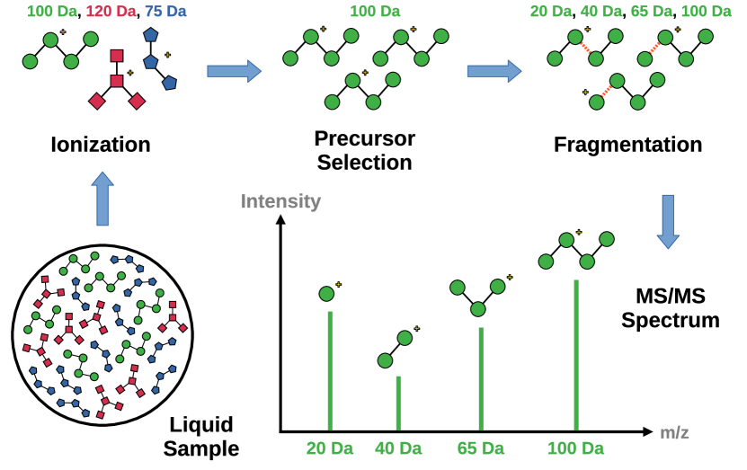
At a high level, tandem mass spectrometry provides information about a molecule’s structure by measuring how it fragments. The experimental process is outlined in Figure 1. First, molecules in the sample are ionized: at this stage they are referred to as precursor ions, because they have not yet undergone fragmentation. In liquid samples, each molecule may become associated with a charged adduct during ionization. For example, if the adduct is a hydrogen ion \ceH+, an \ce[M+\ceH]+ precursor ion will form. Following ionization, the mass to charge ratio () of each precursor ion is subsequently measured using a mass analyzer. After the precursor values are are recorded, ions with a particular are selected for further analysis in the form of fragmentation. The fragmentation process is typically facilitated by energetic collisions with neutral gas particles, and can be influenced by experimental parameters such as collision energy.
After fragmentation, the resulting charged ions are sent back to the mass analyzer for measurement, producing a distribution over fragment values that reflects how often each fragment was formed. Often there are multiple fragments with nearly identical , complicating analysis of the spectrum. Since the fragmentation process is stochastic, an individual precursor ion can break down into different fragments with different probabilities. However, with a sufficiently high precursor ion concentration, enough independent fragmentations can occur such that sampling error is no longer a concern. The mass spectrum is defined as the probability distribution over the fragment values. Since the charge is usually or for small molecules, the spectrum can also be interpreted as a distribution over masses, where each mass is measured in Daltons (Da). Throughout this work, we focus our analysis on \ce[M+\ceH]+ spectra (where is always ), although our methods can easily be extended to other types of precursor ions.
The process of fragmentation involves breakage and formation of bonds between atoms in the molecule. Each fragment is, by definition, composed of a subset of the atoms in the original precursor. Fragmentation is typically modelled as a sequence of high-energy reactions. Generally, a reaction involves a charged fragment (which could be the precursor) being converted into two sub-fragments, only one of which is charged. The neutral (uncharged) sub-fragment is described as a neutral loss because it cannot be measured by the mass spectrometer and ends up getting discarded. The charged sub-fragment may undergo further reactions to produce additional fragments. The most common type of reaction is an -Cleavage, which results in the removal of a single bond. More complicated reactions are possible (McLafferty, 1959; Biemann, 1962; van Tetering et al., 2024), but in many cases these reactions can be approximated as sequences of bond breakages.
Mathematically, a mass spectrum can be represented as a finite set of tuples where each mass has an associated probability . Individual tuples are often referred to as peaks, with the mass being called the peak location and the probability being called the peak intensity. The problem of spectrum prediction can be formulated as a standard supervised learning task. The dataset is composed of tuples where is a molecule and is its associated mass spectrum. The set of masses in a particular spectrum is denoted as . The goal of a C2MS model is to predict from .
3 Related Work
The increasing availability of small molecule MS/MS data has lead to a proliferation of machine learning models for spectrum prediction. Existing methods can be broadly grouped into two categories, binned and structured, based on how they represent the spectrum.
Binned methods approximate the spectrum as a sequence of discrete mass bins with associated peak intensities. This reduces the spectrum prediction problem to a vector regression task, which can be readily solved without extensive domain-specific model customization. Binned approaches generally vary based on the strategy they employ for encoding the input molecule: multi-layer percetprons (Wei et al., 2019), 2D (Zhu et al., 2020; Li et al., 2022) and 3D (Hong et al., 2023) graph neural networks, and graph transformers (Young et al., 2023) have all been used successfully. However, selecting an appropriate bin size can be challenging: bins that are too large result in loss of information, while bins that are too small can be overly sensitive to measurement error and yield high-dimensional spectrum vectors that are impractical to model. This presents a fundamental roadblock for the application of binned models in retrieval-based MS2C.
Structured approaches sidestep the binning problem by modelling the spectrum as a distribution over chemical formulae, whose masses can be calculated trivially with extremely high precision. Some methods predict the formula distribution directly, using either autoregressive formula generation (Goldman et al., 2023a) or a large fixed formula vocabulary (Murphy et al., 2023). Others rely on recursive fragmentation (Wang et al., 2021; Zhu & Jonas, 2023) or autoregressive generation (Goldman et al., 2024) to model a distribution over fragments, which induces a distribution over formulae. While structured MS2C models can generate very high resolution spectra, they tend to be slower than binned approaches due to the increased complexity of the output space.
There is a natural trade-off between a model’s scalability and the amount of information it can provide about the fragmentation process. Methods that infer fragment distributions are most informative, since they explicitly describe how the molecule breaks apart. However, these models tend to involve stronger priors and more complex prediction schemes (Wang et al., 2021; Zhu & Jonas, 2023; Goldman et al., 2024) to facilitate efficient exploration of the combinatorial fragment space. FraGNNet takes a pragmatic approach, achieving a level of interpretability that approaches that of the most sophisticated fragmentation models, while maintaining high performance and scalability (see Appendix C).
4 Methods
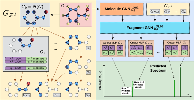
4.1 Overview
The goal of our method is to predict a high resolution MS/MS spectrum based on an input molecular structure. The model works in two stages: first, a heuristic bond-breaking algorithm (Section 4.2) generates a set of plausible molecule fragments. Then, a probabilistic model (Section 4.3) parameterized by a graph neural network (Section 4.4) predicts a distribution over these fragments. The fragment distribution induces a distribution over chemical formulae, which is converted to a mass spectrum by mapping formula masses. This approach allows for extremely high resolution peak predictions with built-in formula and fragment annotations.
4.2 Recursive Fragmentation
A small organic molecule can be represented as an undirected graph . Each node represents an atom in the molecule with an associated element label (where is a finite set of common elements) and each edge represents a covalent bond between atoms. Let be the set of connected subgraphs of the graph .
Definition 4.1.
The graph is called a fragmentation DAG with respect to the graph if the following properties hold:
-
1.
Each node maps to a connected subgraph
-
2.
A directed edge from node to node can exist if and only if is a connected subgraph of .
Note that the root node of always maps to the original graph , and the leaves of correspond to individual atoms .
Most fragments in a mass spectrum can be modelled as products of a series of bond breakages. Such fragments will thus appear as nodes , and their fragmentation history can be represented as a path from the root to . It is possible to derive a set of chemical formulae , where each formula is a -dimensional vector representing the element counts of atoms in . This set can be used to calculate the set of possible peak locations in the spectrum, where is the mass of formula .
The fragmentation DAG can be a useful tool for spectrum prediction (Wang et al., 2021; Goldman et al., 2023a, 2024), providing information about peak locations and relationships between fragments in the spectrum. However, computing from through exhaustive edge removal can be expensive, requiring on the order of operations. Inspired by previous approaches from the literature (Wolf et al., 2010; Ruttkies et al., 2016; Allen et al., 2015; Ridder et al., 2014; Goldman et al., 2024), we approximate using a few simplifying assumptions.
Definition 4.2.
The graph is called a heavy atom skeleton of if is the largest connected subgraph of such that (hydrogen) for all .
Since is often smaller than by a factor of 2-3, calculating is considerably faster than calculating . We employ a recursive edge removal (i.e. bond-breaking) algorithm that only considers nodes that are at most hops away from the root , producing a connected subgraph .
For simplicity of notation, we refer to as , with vertex set and edge set . Since, by definition, each node corresponds to a subgraph that does not contain any hydrogen atoms, we employ a heuristic to model the possible number of hydrogens associated with each . Let be the number of hydrogen atoms in that are connected to the subgraph . We define the set as the range of hydrogen counts for the subgraph , where is a tolerance parameter.
This induces a set of possible formulae and associated masses , where is a formula with the same heavy atom counts as and hydrogens, and is its corresponding mass. Hydrogen transfers are common in fragmentation, so allowing for flexibility in the hydrogen counts can result in a more representative set of formulae.
Definition 4.3.
The set
is the set of masses derived from the approximate heavy-atom fragmentation DAG with hydrogen tolerance .
4.3 Probabilistic Formulation
Our model can be interpreted as a structured latent variable model whose latent distributions depend on a molecular graph and its approximate fragmentation DAG .
To begin, we define the following latent probability distributions:
Definition 4.4.
Let be a discrete finite probability distribution over the DAG nodes , parameterized by a neural network .
Definition 4.5.
Let be a discrete finite conditional distribution between DAG nodes and associated formulae , parameterized by a neural network .
Both distributions depend implicitly on the molecular graph , but for clarity of notation we have omitted this. Note that for each node , has support over formulae.111There is additional filtering for chemical validity which may mask out some formulae, but for clarity this has been omitted.
The joint distribution can be loosely interpreted as identifying which substructures are generated during fragmentation, with modelling the heavy atom structures of the probable fragments and identifying the number of hydrogens associated with each of those fragments.
By marginalizing over the nodes , it is possible to calculate a distribution over formulae . Since each formula has an associated mass, the discrete distribution can be easily converted to a continuous distribution over masses. Following (Allen et al., 2015), we formulate as a mixture of univariate Gaussians as outlined in Equation 1:
| (1) | ||||
The conditional is a narrow truncated Gaussian centered on the formula mass, , with variance proportional to and truncation occurring at standard deviation from the mean. This Gaussian model approximates the typical error distribution of the mass analyzer (Allen et al., 2015). At inference time it is convenient to approximate as a discrete distribution with , where is the Dirac delta function.
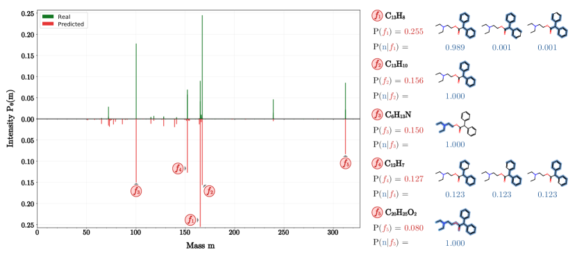
It is possible to calculate another distribution using Bayes Theorem. Intuitively identifies which fragments are contributing to a predicted peak centered at formula – for this reason we refer to it as the peak annotation distribution. While not directly used to generate the spectrum, can be helpful for interpreting model behaviour (see Section 5.3, Figure 3).
In Appendix D, we describe alternate versions of , , and that account for fragment subgraph isomorphism.
4.4 Neural Network Parameterization
The distributions and are parameterized by a two-stage graph neural network (GNN, Battaglia et al. 2018) as defined by Equation 2:
| (2) |
The first stage , called the Molecule GNN, operates on the input molecular graph . The second stage , called the Fragment GNN, combines information from the fragmentation DAG and the molecule embeddings to predict the distributions and .
4.4.1 Molecule GNN
The Molecule GNN takes the input molecular graph and outputs embeddings for the atoms in the graph. The atom embeddings and bond embeddings are initialized with specific features from (see Appendix E).
GNN models work by iteratively updating node states through the aggregation of neighbourhood information. uses the GINE architecture (Xu et al., 2018; Fey & Lenssen, 2019), which incorporates both node and edge information in its updates. The GINE update rule is given by equation 3, where is the GNN layer index, , and is a standard multi-layer perceptron (MLP):
| (3) |
The final atom embeddings are subsequently passed to the Fragment GNN for further processing.
4.4.2 Fragment GNN
The Fragment GNN is another GINE network that propagates information along the approximate fragmentation DAG. Each DAG node is featurized using information about its associated subgraph , precisely described in Equations 4 and 5. The vector is a concatenation of three terms: is the average atom embedding for atoms in ; is an embedding of the subgraph formula ; and is an embedding of the depth in the DAG at which node is located.
| (4) | ||||
| (5) |
The edge embeddings are also initialized with subgraph information: they capture differences between adjacent DAG nodes. Refer to Appendix F for full details.
The DAG nodes are processed by the Fragment GNN in a manner that is similar to Equation 3. After layers of processing, a small output MLP is applied to each node embedding , producing a dimensional vector representing the unnormalized logits for for each . The other latent distributions in Section 4.3 are calculated from the joint through normalization, marginalization, and application of Bayes Theorem.
While performing model ablations (see Appendix H), we discovered that edge information could be omitted without degradation in performance, allowing for 2x faster training and inference. As a result, the experiments in Section 5 use a variant of that excludes the neighbourhood aggregation term from the GINE update.
4.5 Loss Function
We fit the parameters of the model with maximum likelihood estimation, using stochastic gradient descent. The loss function is based on the negative log-likelihood of the data, defined in Equation 6:
| (6) |
For each spectrum, a subset of the peak masses are defined to be Outside of the Support (OS) if they are far enough from away the predicted set of masses such that their predicted probability is 0 (Equation 7). The rest of the masses are deemed to be Inside of the Support (IS).
| (7) |
Modelling the OS probability can provide useful information about the reliability of the predicted spectrum. With slight modification, FraGNNet can be adapted to predict , an estimation of . Adjusting the loss function to incorporate an OS cross-entropy term yields Equation 8:
| (8) |
In cases where , perfectly optimizing yields predictions which have (incorrectly) redistributed to other peaks. This undesirable behaviour can be avoided by minimizing instead.
4.6 Latent Entropy Regularization
Latent entropies can provide insight into the model’s understanding of the fragmentation process. describes the diversity of fragment skeletons that were generated; describes variability in hydrogen configurations for each skeleton; describes variability in peak annotations.
Since entropy is differentiable, joint optimization of latent entropy and prediction error is possible using gradient-based methods. The normalized entropy is preferable for optimization since it accounts for differences in latent support size caused by variations in the size of the input molecule. Incorporating normalized entropy into the objective function, as demonstrated in Equation 9, effectively imposes entropy regularization on the latent distributions:
| (9) |
The tunable hyperparameters control the influence of the entropy regularizers. Since is minimized, setting will maximize the corresponding normalized entropy , and vice versa. Entropy regularization can be useful when assessing consistency of peak annotations, as demonstrated in Section 5.3.
| Split | Model | ||||
|---|---|---|---|---|---|
| InChIKey | FragNet-D4 | ||||
| InChIKey | FragNet-D3 | ||||
| InChIKey | Iceberg-ADV | - | |||
| InChIKey | Iceberg | - | |||
| InChIKey | MassFormer | - | - | - | |
| InChIKey | NEIMS | - | - | - | |
| Scaffold | FragNet-D4 | ||||
| Scaffold | FragNet-D3 | ||||
| Scaffold | Iceberg-ADV | - | |||
| Scaffold | Iceberg | - | |||
| Scaffold | MassFormer | - | - | - | |
| Scaffold | NEIMS | - | - | - |
5 Experiments
5.1 Spectrum Prediction (C2MS)
FraGNNet’s C2MS performance is evaluated on a heldout portion of the NIST20 MS/MS dataset (Appendix I), to allow for comparison with other binned and structured prediction models from the literature.
ICEBERG (Goldman et al., 2024) is a structured method for high-resolution spectrum prediction that uses a two-stage model. The first stage autoregressively predicts a set of fragments, and the second stage predicts a mapping between those fragments and the peaks in the spectrum (see Appendix C). The stages are trained independently, with the first stage approximating the output of a heuristic fragmenter, MAGMa (Ridder et al., 2014), that uses signals from the spectrum to find a minimal set of fragments that explain the peaks. We introduce ICEBERG-ADV (advantaged), a variant of ICEBERG that replaces the first stage of the model with the exact MAGMa output. This modification removes sampling error in the fragment generation process, creating an artificially easier learning problem that should result in better performance. We emphasize that ICEBERG-ADV is only suitable for benchmarking: in most realistic C2MS problems ground truth spectra are not available at inference time, meaning that MAGMa cannot be applied.
The other baseline models, MassFormer (Young et al., 2023) and NEIMS (Wei et al., 2019), both predict binned spectra at a lower resolution. The former uses a pretrained graph transformer model (Ying et al., 2021) to encode the molecule, while the latter relies on domain-specific chemical fingerprint representations (Rogers & Hahn, 2010).
The results are summarized in Table 1. FraGNNet-D4, a version of our model that uses a approximation of the fragmentation DAG, clearly outperforms other models in terms of cosine similarity. The binned spectrum approaches (NEIMS and MassFormer) score much worse in terms of cosine hungarian similarity (Appendix G) due to the limited resolution afforded by their binned spectrum representation.
Increasing fragmentation depth from to seems to have a positive impact on performance. Lower with FraGNNet-D4 is indicative of better mass coverage when compared to FraGNNet-D3, leading to better similarity scores. Both models are able to estimate to some degree, suggesting that FraGNNet can identify situations at inference time where its fragmentation model will be inaccurate.
5.2 Compound Retrieval (MS2C)
FraGNNet was also evaluated in a retrieval-based MS2C task. Our setup is similar to previous methods (Goldman et al., 2024; Murphy et al., 2023): for each in the NIST20 Test set (roughly 4000 pairs, Appendix I) a candidate set is constructed from and 49 other compounds sampled from PubChem (Kim et al., 2019). Each is selected to have high chemical similarity with as measured by Tanimoto similarity between chemical fingerprints (Rogers & Hahn, 2010). The C2MS models are tasked with predicting a set of spectra for molecules . The spectra are ranked by their cosine hungarian similarity (Appendix G) with the real spectrum , inducing a ranking on the molecules . The models are scored based on their ability to correctly rank in the Top- for . FraGNNet outperform all baseline models for for all values of (see Tables 2 and 8).
| Model | Top-1 | Top-3 | Top-5 | Top-10 |
|---|---|---|---|---|
| FraGNNet-D4 | ||||
| FraGNNet-D3 | ||||
| ICEBERG | ||||
| MassFormer | ||||
| NEIMS |
5.3 Annotation Consistency
When interpreting mass spectral data, practitioners will annotate each peak in the spectrum with a substructure to explain what happened during fragmentation. FraGNNet’s latent distribution provides a map from formulae to DAG nodes and their associated subgraphs . can be interpreted as a peak annotation distribution (see Figure 3 for an example), with the mode identifying the subgraph that contributes most to the peak located at .
It is difficult to evaluate the correctness of peak annotations (human-derived or otherwise) without additional experimental analysis (van Tetering et al., 2024). However, we can measure the consistency of annotations across models that perform equally well. Inter-model differences in latent distributions that do not affect overall C2MS performance are indicative of ambiguity in the fragmentation process. Similar to how ensembles can be used to estimate prediction uncertainty (Lakshminarayanan et al., 2017), identifying annotation inconsistencies across a group of models with comparable average performance could be a useful strategy for flagging unreliable annotations.
To investigate annotation consistency, we trained two separate ensembles of 15 FraGNNet-D3 models. The Standard Ensemble is composed of models without entropy regularization (). The Entropy Ensemble is composed of five models with high entropy (), five models with low entropy (), and five models without regularization (). Aside from entropy regularization, all models use the same optimization hyperparameters and only differ by initialization seed.
| Metric | Entropy Ens | Standard Ens |
|---|---|---|
| Mean | ||
| CV | ||
| Mean | ||
| CV | ||
| Cons | ||
| Maj |
Table 3 demonstrates how these two ensembles achieve comparable average cosine similarity, but differ significantly in annotation distribution . The Entropy Ensemble experiences more variability in latent entropy , with a coefficient of variation that is roughly twice as large as that of the Standard Ensemble. Trends in entropy are reflected in annotation agreement: the Entropy Ensemble has a lower average rate of annotation consensus than the Standard Ensemble (0.745 vs 0.818). Additionally, the average fraction of individual models that agree with the ensemble majority vote is lower in the Entropy Ensemble (0.922 vs 0.939). These trends are also reflected in the isomorphic annotation distribution (Appendix J), although the entropy variations and resulting annotation disagreements are lower in comparison to those associated with .
Altogether, these results demonstrate how ensembles can be used to identify unreliable FraGNNet structure annotations. Furthermore, they suggest that ensembling models with different latent entropies can improve sensitivity to annotation ambiguity without sacrificing performance.
6 Discussion
In this work we introduce FraGNNet, a deep probabilistic model for spectrum prediction. Our work shows that pairing combinatorial fragmentation with neural networks can achieve state-of-the-art C2MS performance. FraGNNet is unique in its interpretable latent representation of the fragmentation DAG. Features such as OS prediction and tunable entropy regularization further differentiate it from existing models. Strong results in the compound retrieval task demonstrate potential utility in MS2C applications.
Several aspects of our approach could be improved. The DAG calculation is a computational bottleneck, requiring recursive bond-removal operations. Additionally, the presence of OS peaks are a reflection of an imperfect fragmentation model, which cannot be fixed with better optimization or more data. Complex reactions like cyclizations are difficult to model, since they introduce an explosion in the size of the fragment space. Developing a method that samples chemical reactions could be a viable solution for identifying fragments that cannot be generated by simple bond-breaking. Alternatively, ensembling FraGNNet with a more flexible C2MS model, such as a binned predictor, could be an effective method of capturing OS peaks. Finally, adding support for unmerged spectrum prediction and increasing precursor adduct coverage are straightforward improvements that would broaden FraGNNet’s practical applicability to MS2C tasks.
References
- Allen et al. (2015) Allen, F., Greiner, R., and Wishart, D. Competitive fragmentation modeling of ESI-MS/MS spectra for putative metabolite identification. Metabolomics, 11(1):98–110, February 2015. ISSN 1573-3890. doi: 10.1007/s11306-014-0676-4. URL https://doi.org/10.1007/s11306-014-0676-4.
- Battaglia et al. (2018) Battaglia, P. W., Hamrick, J. B., Bapst, V., Sanchez-Gonzalez, A., Zambaldi, V., Malinowski, M., Tacchetti, A., Raposo, D., Santoro, A., Faulkner, R., Gulcehre, C., Song, F., Ballard, A., Gilmer, J., Dahl, G., Vaswani, A., Allen, K., Nash, C., Langston, V., Dyer, C., Heess, N., Wierstra, D., Kohli, P., Botvinick, M., Vinyals, O., Li, Y., and Pascanu, R. Relational inductive biases, deep learning, and graph networks. arXiv:1806.01261 [cs, stat], October 2018. URL http://arxiv.org/abs/1806.01261.
- Behnel et al. (2011) Behnel, S., Bradshaw, R., Citro, C., Dalcin, L., Seljebotn, D. S., and Smith, K. Cython: The best of both worlds. Computing in Science & Engineering, 13(2):31–39, 2011.
- Bemis & Murcko (1996) Bemis, G. W. and Murcko, M. A. The Properties of Known Drugs. 1. Molecular Frameworks. Journal of Medicinal Chemistry, 39(15):2887–2893, January 1996. ISSN 0022-2623. doi: 10.1021/jm9602928. URL https://doi.org/10.1021/jm9602928.
- Biemann (1962) Biemann, K. The application of mass spectrometry in organic chemistry: Determination of the structure of natural products. Angewandte Chemie International Edition in English, 1(2):98–111, 1962. doi: https://doi.org/10.1002/anie.196200981. URL https://onlinelibrary.wiley.com/doi/abs/10.1002/anie.196200981.
- Biewald (2020) Biewald, L. Experiment tracking with weights and biases, 2020. URL https://www.wandb.com/. Software available from wandb.com.
- Butler et al. (2023) Butler, T., Frandsen, A., Lightheart, R., Bargh, B., Taylor, J., Bollerman, T. J., Kerby, T., West, K., Voronov, G., Moon, K., Kind, T., Dorrestein, P., Allen, A., Colluru, V., and Healey, D. MS2mol: A transformer model for illuminating dark chemical space from mass spectra, 2023. URL https://chemrxiv.org/engage/chemrxiv/article-details/6492507524989702c2b082fc.
- Dueñas et al. (2022) Dueñas, M. E., Peltier‐Heap, R. E., Leveridge, M., Annan, R. S., Büttner, F. H., and Trost, M. Advances in high‐throughput mass spectrometry in drug discovery. EMBO Molecular Medicine, 15(1):e14850, December 2022. ISSN 1757-4676. doi: 10.15252/emmm.202114850. URL https://www.ncbi.nlm.nih.gov/pmc/articles/PMC9832828/.
- Dührkop et al. (2015) Dührkop, K., Shen, H., Meusel, M., Rousu, J., and Böcker, S. Searching molecular structure databases with tandem mass spectra using csi:fingerid. Proceedings of the National Academy of Sciences, 112(41):12580–12585, 2015. ISSN 0027-8424. doi: 10.1073/pnas.1509788112. URL https://www.pnas.org/content/112/41/12580.
- Durant et al. (2002) Durant, J. L., Leland, B. A., Henry, D. R., and Nourse, J. G. Reoptimization of MDL keys for use in drug discovery. Journal of Chemical Information and Computer Sciences, 42(6):1273–1280, 2002. ISSN 0095-2338. doi: 10.1021/ci010132r.
- Dührkop et al. (2019) Dührkop, K., Fleischauer, M., Ludwig, M., Aksenov, A. A., Melnik, A. V., Meusel, M., Dorrestein, P. C., Rousu, J., and Böcker, S. SIRIUS 4: a rapid tool for turning tandem mass spectra into metabolite structure information. Nature Methods, 16(4):299–302, April 2019. ISSN 1548-7105. doi: 10.1038/s41592-019-0344-8. URL http://www.nature.com/articles/s41592-019-0344-8.
- Falcon & The PyTorch Lightning team (2019) Falcon, W. and The PyTorch Lightning team. PyTorch Lightning, March 2019. URL https://github.com/Lightning-AI/lightning.
- Fey & Lenssen (2019) Fey, M. and Lenssen, J. E. Fast graph representation learning with pytorch geometric. CoRR, abs/1903.02428, 2019. URL http://arxiv.org/abs/1903.02428.
- Goldman et al. (2023a) Goldman, S., Bradshaw, J., Xin, J., and Coley, C. Prefix-Tree Decoding for Predicting Mass Spectra from Molecules. In Oh, A., Neumann, T., Globerson, A., Saenko, K., Hardt, M., and Levine, S. (eds.), Advances in Neural Information Processing Systems, volume 36, pp. 48548–48572. Curran Associates, Inc., 2023a. URL https://proceedings.neurips.cc/paper_files/paper/2023/file/97d596ca21d0751ba2c633bad696cf7f-Paper-Conference.pdf.
- Goldman et al. (2023b) Goldman, S., Wohlwend, J., Stražar, M., Haroush, G., Xavier, R. J., and Coley, C. W. Annotating metabolite mass spectra with domain-inspired chemical formula transformers. Nature Machine Intelligence, 5(9):965–979, 2023b. ISSN 2522-5839. doi: 10.1038/s42256-023-00708-3. URL https://www.nature.com/articles/s42256-023-00708-3. Number: 9 Publisher: Nature Publishing Group.
- Goldman et al. (2023c) Goldman, S., Xin, J., Provenzano, J., and Coley, C. W. MIST-CF: Chemical Formula Inference from Tandem Mass Spectra. Journal of Chemical Information and Modeling, September 2023c. ISSN 1549-9596. doi: 10.1021/acs.jcim.3c01082. URL https://doi.org/10.1021/acs.jcim.3c01082. Publisher: American Chemical Society.
- Goldman et al. (2024) Goldman, S., Li, J., and Coley, C. W. Generating Molecular Fragmentation Graphs with Autoregressive Neural Networks. Analytical Chemistry, 96(8):3419–3428, February 2024. ISSN 0003-2700. doi: 10.1021/acs.analchem.3c04654. URL https://doi.org/10.1021/acs.analchem.3c04654. Publisher: American Chemical Society.
- Gowda & Djukovic (2014) Gowda, G. N. and Djukovic, D. Overview of Mass Spectrometry-Based Metabolomics: Opportunities and Challenges. Methods in molecular biology (Clifton, N.J.), 1198:3–12, 2014. ISSN 1064-3745. doi: 10.1007/978-1-4939-1258-2“˙1. URL https://www.ncbi.nlm.nih.gov/pmc/articles/PMC4336784/.
- Hagberg et al. (2008) Hagberg, A., Swart, P., and S Chult, D. Exploring network structure, dynamics, and function using networkx. Technical report, Los Alamos National Lab.(LANL), Los Alamos, NM (United States), 2008.
- Heller et al. (2015) Heller, S. R., McNaught, A., Pletnev, I., Stein, S., and Tchekhovskoi, D. InChI, the IUPAC International Chemical Identifier. Journal of Cheminformatics, 7(1):23, May 2015. ISSN 1758-2946. doi: 10.1186/s13321-015-0068-4. URL https://doi.org/10.1186/s13321-015-0068-4.
- Hong et al. (2023) Hong, Y., Li, S., Welch, C. J., Tichy, S., Ye, Y., and Tang, H. 3DMolMS: prediction of tandem mass spectra from 3D molecular conformations. Bioinformatics, 39(6):btad354, May 2023. ISSN 1367-4811. doi: 10.1093/bioinformatics/btad354. URL https://doi.org/10.1093/bioinformatics/btad354. _eprint: https://academic.oup.com/bioinformatics/article-pdf/39/6/btad354/50661428/btad354.pdf.
- Huber et al. (2020) Huber, F., Verhoeven, S., Meijer, C., Spreeuw, H., Castilla, E. M. V., Geng, C., Hooft, J. J. j. v. d., Rogers, S., Belloum, A., Diblen, F., and Spaaks, J. H. matchms - processing and similarity evaluation of mass spectrometry data. Journal of Open Source Software, 5(52):2411, August 2020. ISSN 2475-9066. doi: 10.21105/joss.02411. URL https://joss.theoj.org/papers/10.21105/joss.02411.
- Kim et al. (2019) Kim, S., Chen, J., Cheng, T., Gindulyte, A., He, J., He, S., Li, Q., Shoemaker, B. A., Thiessen, P. A., Yu, B., Zaslavsky, L., Zhang, J., and Bolton, E. E. PubChem 2019 update: improved access to chemical data. Nucleic Acids Research, 47(Database issue):D1102–D1109, January 2019. ISSN 0305-1048. doi: 10.1093/nar/gky1033. URL https://www.ncbi.nlm.nih.gov/pmc/articles/PMC6324075/.
- Kong et al. (2022) Kong, K., Li, G., Ding, M., Wu, Z., Zhu, C., Ghanem, B., Taylor, G., and Goldstein, T. Robust optimization as data augmentation for large-scale graphs. In Proceedings of the IEEE/CVF Conference on Computer Vision and Pattern Recognition, pp. 60–69, 2022.
- Kuhn (1955) Kuhn, H. W. The Hungarian method for the assignment problem. Naval Research Logistics Quarterly, 2(1-2):83–97, March 1955. ISSN 0028-1441, 1931-9193. doi: 10.1002/nav.3800020109. URL https://onlinelibrary.wiley.com/doi/10.1002/nav.3800020109.
- Lakshminarayanan et al. (2017) Lakshminarayanan, B., Pritzel, A., and Blundell, C. Simple and Scalable Predictive Uncertainty Estimation using Deep Ensembles. In Advances in Neural Information Processing Systems, volume 30. Curran Associates, Inc., 2017. URL https://proceedings.neurips.cc/paper_files/paper/2017/hash/9ef2ed4b7fd2c810847ffa5fa85bce38-Abstract.html.
- Landrum (2022) Landrum, G. Rdkit: Open-source cheminformatics, 2022. URL http://www.rdkit.org.
- Lebedev (2013) Lebedev, A. T. Environmental Mass Spectrometry. Annual Review of Analytical Chemistry, 6(1):163–189, 2013. doi: 10.1146/annurev-anchem-062012-092604. URL https://doi.org/10.1146/annurev-anchem-062012-092604.
- Li et al. (2022) Li, X., Zhu, H., Liu, L.-p., and Hassoun, S. Ensemble Spectral Prediction (ESP) Model for Metabolite Annotation. arXiv:2203.13783 [cs, q-bio], March 2022. URL http://arxiv.org/abs/2203.13783. arXiv: 2203.13783.
- McLafferty (1959) McLafferty, F. W. Mass Spectrometric Analysis. Molecular Rearrangements. Analytical Chemistry, 31(1):82–87, January 1959. ISSN 0003-2700. doi: 10.1021/ac60145a015. URL https://doi.org/10.1021/ac60145a015. Publisher: American Chemical Society.
- Murphy et al. (2023) Murphy, M., Jegelka, S., Fraenkel, E., Kind, T., Healey, D., and Butler, T. Efficiently predicting high resolution mass spectra with graph neural networks. In Krause, A., Brunskill, E., Cho, K., Engelhardt, B., Sabato, S., and Scarlett, J. (eds.), Proceedings of the 40th International Conference on Machine Learning, volume 202 of Proceedings of Machine Learning Research, pp. 25549–25562. PMLR, July 2023. URL https://proceedings.mlr.press/v202/murphy23a.html.
- Nakata & Shimazaki (2017) Nakata, M. and Shimazaki, T. PubChemQC Project: A Large-Scale First-Principles Electronic Structure Database for Data-Driven Chemistry. Journal of Chemical Information and Modeling, 57(6):1300–1308, June 2017. ISSN 1549-9596. doi: 10.1021/acs.jcim.7b00083. URL https://doi.org/10.1021/acs.jcim.7b00083.
- Paszke et al. (2019) Paszke, A., Gross, S., Massa, F., Lerer, A., Bradbury, J., Chanan, G., Killeen, T., Lin, Z., Gimelshein, N., Antiga, L., Desmaison, A., Köpf, A., Yang, E., DeVito, Z., Raison, M., Tejani, A., Chilamkurthy, S., Steiner, B., Fang, L., Bai, J., and Chintala, S. PyTorch: An Imperative Style, High-Performance Deep Learning Library. arXiv:1912.01703 [cs, stat], December 2019. URL http://arxiv.org/abs/1912.01703.
- Peters (2011) Peters, F. T. Recent advances of liquid chromatography–(tandem) mass spectrometry in clinical and forensic toxicology. Clinical Biochemistry, 44(1):54–65, January 2011. ISSN 0009-9120. doi: 10.1016/j.clinbiochem.2010.08.008. URL https://www.sciencedirect.com/science/article/pii/S0009912010003486.
- Python Core Team (2021) Python Core Team. Python: A dynamic, open source programming language. Python Software Foundation, 2021. URL https://www.python.org/.
- Ridder et al. (2014) Ridder, L., Hooft, J. J. J. v. d., and Verhoeven, S. Automatic Compound Annotation from Mass Spectrometry Data Using MAGMa. Mass Spectrometry, 3(Special_Issue_2):S0033–S0033, 2014. doi: 10.5702/massspectrometry.S0033.
- Rogers & Hahn (2010) Rogers, D. and Hahn, M. Extended-Connectivity Fingerprints. Journal of Chemical Information and Modeling, 50(5):742–754, May 2010. ISSN 1549-9596. doi: 10.1021/ci100050t. URL https://doi.org/10.1021/ci100050t.
- Ruttkies et al. (2016) Ruttkies, C., Schymanski, E. L., Wolf, S., Hollender, J., and Neumann, S. MetFrag relaunched: incorporating strategies beyond in silico fragmentation. Journal of Cheminformatics, 8(1):3, January 2016. ISSN 1758-2946. doi: 10.1186/s13321-016-0115-9. URL https://doi.org/10.1186/s13321-016-0115-9.
- Schymanski et al. (2017) Schymanski, E. L., Ruttkies, C., Krauss, M., Brouard, C., Kind, T., Dührkop, K., Allen, F., Vaniya, A., Verdegem, D., Böcker, S., Rousu, J., Shen, H., Tsugawa, H., Sajed, T., Fiehn, O., Ghesquière, B., and Neumann, S. Critical Assessment of Small Molecule Identification 2016: automated methods. Journal of Cheminformatics, 9(1):22, March 2017. ISSN 1758-2946. doi: 10.1186/s13321-017-0207-1. URL https://doi.org/10.1186/s13321-017-0207-1.
- Shervashidze et al. (2011) Shervashidze, N., Schweitzer, P., Leeuwen, E. J. v., Mehlhorn, K., and Borgwardt, K. M. Weisfeiler-Lehman Graph Kernels. Journal of Machine Learning Research, 12(77):2539–2561, 2011. URL http://jmlr.org/papers/v12/shervashidze11a.html.
- Shrivastava et al. (2021) Shrivastava, A. D., Swainston, N., Samanta, S., Roberts, I., Wright Muelas, M., and Kell, D. B. MassGenie: A Transformer-Based Deep Learning Method for Identifying Small Molecules from Their Mass Spectra. Biomolecules, 11(12):1793, November 2021. ISSN 2218-273X. doi: 10.3390/biom11121793. URL https://www.ncbi.nlm.nih.gov/pmc/articles/PMC8699281/.
- Skinnider et al. (2021) Skinnider, M. A., Wang, F., Pasin, D., Greiner, R., Foster, L. J., Dalsgaard, P. W., and Wishart, D. S. A deep generative model enables automated structure elucidation of novel psychoactive substances. Nature Machine Intelligence, 3(11):973–984, November 2021. ISSN 2522-5839. doi: 10.1038/s42256-021-00407-x. URL https://www.nature.com/articles/s42256-021-00407-x. Number: 11 Publisher: Nature Publishing Group.
- Stein (2012) Stein, S. Mass Spectral Reference Libraries: An Ever-Expanding Resource for Chemical Identification. Analytical Chemistry, 84(17):7274–7282, September 2012. ISSN 0003-2700. doi: 10.1021/ac301205z. URL https://doi.org/10.1021/ac301205z.
- Stein & Scott (1994) Stein, S. E. and Scott, D. R. Optimization and testing of mass spectral library search algorithms for compound identification. Journal of the American Society for Mass Spectrometry, 5(9):859–866, September 1994. ISSN 1044-0305. doi: 10.1016/1044-0305(94)87009-8. URL https://pubs.acs.org/doi/10.1016/1044-0305%2894%2987009-8.
- Stravs et al. (2022) Stravs, M. A., Dührkop, K., Böcker, S., and Zamboni, N. MSNovelist: de novo structure generation from mass spectra. Nature Methods, 19(7):865–870, July 2022. ISSN 1548-7105. doi: 10.1038/s41592-022-01486-3. URL https://www.nature.com/articles/s41592-022-01486-3. Number: 7 Publisher: Nature Publishing Group.
- Tancik et al. (2020) Tancik, M., Srinivasan, P. P., Mildenhall, B., Fridovich-Keil, S., Raghavan, N., Singhal, U., Ramamoorthi, R., Barron, J. T., and Ng, R. Fourier features let networks learn high frequency functions in low dimensional domains. CoRR, abs/2006.10739, 2020. URL https://arxiv.org/abs/2006.10739.
- van Tetering et al. (2024) van Tetering, L., Spies, S., Wildeman, Q. D. K., Houthuijs, K. J., van Outersterp, R. E., Martens, J., Wevers, R. A., Wishart, D. S., Berden, G., and Oomens, J. A spectroscopic test suggests that fragment ion structure annotations in MS/MS libraries are frequently incorrect. Communications Chemistry, 7(1):1–11, February 2024. ISSN 2399-3669. doi: 10.1038/s42004-024-01112-7. URL https://www.nature.com/articles/s42004-024-01112-7. Number: 1 Publisher: Nature Publishing Group.
- Voronov et al. (2022) Voronov, G., Frandsen, A., Bargh, B., Healey, D., Lightheart, R., Kind, T., Dorrestein, P., Colluru, V., and Butler, T. Ms2prop: A machine learning model that directly predicts chemical properties from mass spectrometry data for novel compounds. bioRxiv, 2022. doi: 10.1101/2022.10.09.511482. URL https://www.biorxiv.org/content/early/2022/10/11/2022.10.09.511482.
- Wang et al. (2021) Wang, F., Liigand, J., Tian, S., Arndt, D., Greiner, R., and Wishart, D. S. CFM-ID 4.0: More Accurate ESI-MS/MS Spectral Prediction and Compound Identification. Analytical Chemistry, August 2021. ISSN 0003-2700. doi: 10.1021/acs.analchem.1c01465. URL https://doi.org/10.1021/acs.analchem.1c01465.
- Wang et al. (2023) Wang, F., Pasin, D., Skinnider, M. A., Liigand, J., Kleis, J.-N., Brown, D., Oler, E., Sajed, T., Gautam, V., Harrison, S., Greiner, R., Foster, L. J., Dalsgaard, P. W., and Wishart, D. S. Deep Learning-Enabled MS/MS Spectrum Prediction Facilitates Automated Identification Of Novel Psychoactive Substances. Analytical Chemistry, 95(50):18326–18334, December 2023. ISSN 0003-2700. doi: 10.1021/acs.analchem.3c02413. URL https://doi.org/10.1021/acs.analchem.3c02413. Publisher: American Chemical Society.
- Wei et al. (2019) Wei, J. N., Belanger, D., Adams, R. P., and Sculley, D. Rapid prediction of electron–ionization mass spectrometry using neural networks. ACS Central Science, 5(4):700–708, April 2019. ISSN 2374-7943, 2374-7951. doi: 10.1021/acscentsci.9b00085. URL https://pubs.acs.org/doi/10.1021/acscentsci.9b00085.
- Wishart et al. (2018) Wishart, D. S., Feunang, Y. D., Marcu, A., Guo, A. C., Liang, K., Vázquez-Fresno, R., Sajed, T., Johnson, D., Li, C., Karu, N., Sayeeda, Z., Lo, E., Assempour, N., Berjanskii, M., Singhal, S., Arndt, D., Liang, Y., Badran, H., Grant, J., Serra-Cayuela, A., Liu, Y., Mandal, R., Neveu, V., Pon, A., Knox, C., Wilson, M., Manach, C., and Scalbert, A. HMDB 4.0: the human metabolome database for 2018. Nucleic Acids Research, 46(D1):D608–D617, January 2018. ISSN 1362-4962. doi: 10.1093/nar/gkx1089.
- Wolf et al. (2010) Wolf, S., Schmidt, S., Müller-Hannemann, M., and Neumann, S. In silico fragmentation for computer assisted identification of metabolite mass spectra. BMC Bioinformatics, 11(1):148, March 2010. ISSN 1471-2105. doi: 10.1186/1471-2105-11-148. URL https://doi.org/10.1186/1471-2105-11-148.
- Wu et al. (2018) Wu, Z., Ramsundar, B., Feinberg, E. N., Gomes, J., Geniesse, C., Pappu, A. S., Leswing, K., and Pande, V. MoleculeNet: a benchmark for molecular machine learning. Chemical Science, 9(2):513–530, January 2018. ISSN 2041-6539. doi: 10.1039/C7SC02664A. URL https://pubs.rsc.org/en/content/articlelanding/2018/sc/c7sc02664a. Publisher: The Royal Society of Chemistry.
- Xu et al. (2018) Xu, K., Hu, W., Leskovec, J., and Jegelka, S. How Powerful are Graph Neural Networks? September 2018. URL https://openreview.net/forum?id=ryGs6iA5Km.
- Yang et al. (2014) Yang, X., Neta, P., and Stein, S. E. Quality Control for Building Libraries from Electrospray Ionization Tandem Mass Spectra. Analytical Chemistry, 86(13):6393–6400, July 2014. ISSN 0003-2700, 1520-6882. doi: 10.1021/ac500711m. URL https://pubs.acs.org/doi/10.1021/ac500711m.
- Ying et al. (2021) Ying, C., Cai, T., Luo, S., Zheng, S., Ke, G., He, D., Shen, Y., and Liu, T.-Y. Do transformers really perform bad for graph representation? Neural Information Processing Systems (NeurIPS), 2021.
- Young et al. (2023) Young, A., Wang, B., and Röst, H. MassFormer: Tandem Mass Spectrum Prediction for Small Molecules using Graph Transformers, May 2023. URL http://arxiv.org/abs/2111.04824. arXiv:2111.04824 [cs, q-bio].
- Zhu et al. (2020) Zhu, H., Liu, L., and Hassoun, S. Using Graph Neural Networks for Mass Spectrometry Prediction. arXiv:2010.04661 [cs], October 2020. URL http://arxiv.org/abs/2010.04661.
- Zhu & Jonas (2023) Zhu, R. L. and Jonas, E. Rapid Approximate Subset-Based Spectra Prediction for Electron Ionization–Mass Spectrometry. Analytical Chemistry, 95(5):2653–2663, February 2023. ISSN 0003-2700. doi: 10.1021/acs.analchem.2c02093. URL https://doi.org/10.1021/acs.analchem.2c02093. Publisher: American Chemical Society.
Appendix A Recursive Fragmentation Algorithm
The approximate fragmentation DAG is constructed by calling Algorithm 1 on the heavy-atom skeleton of the molecule , with initial depth parameter . BFSCC is a breadth-first search algorithm that returns the set of nodes and edges in a graph that can be reached from a given input node. ID is a function that takes a subset of the (ordered) graph nodes and maps them to a unique integer id (our implementation simply converts the binary representation of the subgraph node mask to a decimal integer).
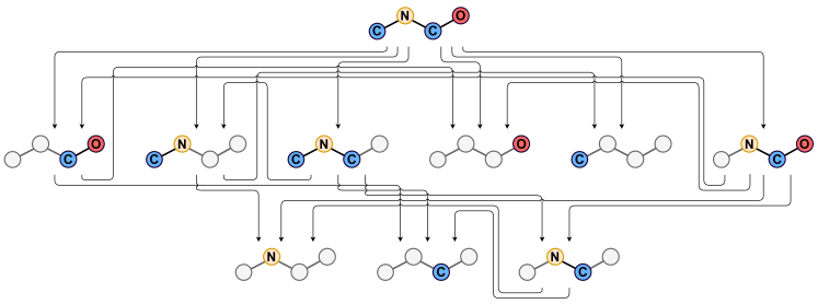
Figure 4 is a visualization of the full fragmentation DAG for an example molecule. Since this molecule is small and linear, the resulting DAG consists of only 10 nodes and 19 edges.
Appendix B Fragmentation DAG Statistics
| Statistic | ||
|---|---|---|
| # Formulae | ||
| # Nodes | ||
| # Nodes | ||
| # Edges | ||
| Recall (0.01 Da) | ||
| Recall (10 ppm) | ||
| Weighted recall (0.01 Da) | ||
| Weighted recall (10 ppm) |
Table 4 describes the size of approximate fragmentation DAG and the coverage of its associated mass set under two different parameterizations. is the configuration used by FraGNNet-D3, and is the configuration for FraGNNet-D4.
Recall () is measured as the fraction of peaks in the spectrum that can be explained by a mass (Equation 10) while weighted recall () incorporates peak intensities (Equation 11).
| (10) |
| (11) |
For the 0.01 Da approach , while for the 10 ppm approach . In our experiments, the output distribution is defined such that iff . Under this definition of the output distribution, weighted recall with 10ppm tolerance is equivalent to the probability .
Appendix C Conceptual Comparisons with Related C2MS Models
In this section, we contrast FraGNNet with two other closely-related structured C2MS models: CFM and ICEBERG.
CFM (Competitive Fragmentation Modelling, Allen et al. 2015; Wang et al. 2021) is the most widely used C2MS tool. Like FraGNNet, it uses a combinatorially generated fragmentation DAG to model a distribution over fragments. However, the level of detail in the DAG is much greater. CFM explicitly models the location of hydrogens and higher order bonds, and implements several complex fragmentation reactions (McLafferty, 1959; Biemann, 1962) that our method does not. In principle, CFM can produce higher quality peak annotations than FraGNNet, since each fragment is (likely) a valid chemical chemical structure and not simply a heavy-atom subgraph and associated hydrogen count. However, this interpretability comes at a cost: the DAG construction step can last over an hour for very large molecules due to its complexity. We do not directly compare with CFM due to difficulties in scaling the model training to larger datasets such as NIST20 (Goldman et al., 2023a, 2024; Murphy et al., 2023). Furthermore, previous work from the literature has demonstrated that it is outperformed by more recent C2MS models (Young et al., 2023; Murphy et al., 2023; Goldman et al., 2024).
ICEBERG (Inferring Collision-induced-dissociation by Estimating Breakage Events and Reconstructing their Graphs, Goldman et al. 2024) is a state-of-the-art C2MS model. As outlined in Section 5.1, ICEBERG is composed of two sub-modules. The first module (the fragment generator) autoregressively predicts a simplified fragmentation DAG, and the second module (the intensity predictor) outputs a distribution over those fragments. The fragment generator is trained to approximate a fragmentation tree that is constructed by a variant of the MAGMa algorithm (Ridder et al., 2014). MAGMa applies a combinatorial atom removal strategy to generate a fragmentation DAG from an input molecular graph : the resulting DAG has a similar set of fragment nodes to , but may contain different edges (refer to Ridder et al. 2014; Goldman et al. 2024 for full details). The MAGMa DAG is then simplified using a number of pruning strategies. Fragments with masses that are not represented by any peak in the spectrum are removed, as are fragments that map to same peak as another (chemical heuristics are used to determine which fragment should be kept in such cases). Unlike our approach, no distinction is made between isomorphic fragments that originate from different parts of the molecule. Redundant paths between fragments are removed to convert the DAG into a proper tree, which is required for autoregressive generation.
ICEBERG’s aggressive pruning removes information from the DAG that could be important for correctly predicting the spectrum. However, this pruning also facilitates more expressive representations of the fragments that remain: since the total number of fragments is lower, the computational and memory cost per fragment can be much higher. This tradeoff underlines the key conceptual difference between FraGNNet and ICEBERG. The former uses a more complete fragmentation DAG but must employ a simpler representation for each individual fragment. The latter can afford a more complex fragment representation but only considers a small subset of the DAG. Our experiments in Section 5.1 suggest that retaining DAG information may be important, since FraGNNet outperforms both ICEBERG (which uses a stochastic approximation to the pruned DAG) and ICEBERG-ADV (which uses extra information from the spectrum to exactly calculate the pruned DAG).
Note that DAG node pruning might also affect predicted peak annotations. Our experiments in Section 5.3 suggest that it is plausible for a single peak to map to multiple fragments, as indicated by non-zero annotation entropies . Compared to FraGNNet, ICEBERG is much more restricted in its ability to model such fragments, preventing it from considering the entire set of plausible annotations.
Appendix D Fragment Subgraph Isomorphism
In mass spectrometry, it is possible for fragments with identical molecular structure to originate from different parts of the molecular graph, having been created through distinct sequences of fragmentation steps. In our model, this phenomenon is represented by pairs of DAG nodes whose corresponding subgraphs are isomorphic (i.e. there exists a node bijection between and that is both label-preserving and edge-preserving).
With the exception of (which does not involve fragments), each of the latent distributions from Section 4.3 can be adapted to account for fragment graph isomorphism. To describe this process precisely, we rely on Definition D.1 and Corollary D.2:
Definition D.1.
Let be a finite set of labelled graphs . Each is a member of one of isomorphism classes , . Assume an arbitrary total ordering for each isomorphic class . Let be the set of graphs such that .
Corollary D.2.
.
For each DAG node such that , we define as the total probability of all subgraphs isomorphic to using Equation 12:
| (12) |
The conditional distributions and are defined in a similar manner using Equations 13 and 14 respectively:
| (13) | ||||
| (14) |
These distributions can provide additional insight into model behaviour, as demonstrated in Appendix J. Intuitively, they remove excess entropy caused by uncertainty over the location in the molecule from which a particular fragment originated.
Appendix E Molecule Features
| Feature | Values |
|---|---|
| Atom Type (Element) | |
| Atom Degree | |
| Atom Orbital Hybridization | |
| Atom Formal Charge | |
| Atom Radical State | |
| Atom Ring Membership | |
| Atom Aromatic | |
| Atom Mass | |
| Atom Chirality | |
| Bond Degree |
Appendix F Fragment Features
F.1 Fourier Embeddings
We use Fourier embeddings (Goldman et al., 2023a; Tancik et al., 2020) to represent certain ordinal features such as mass formulae and collision energies. Given an integer feature , the corresponding Fourier embedding can be calculated using Equation 15:
| (15) |
In principle, it may be easier for the model to handle inputs at inference that have not been seen in training when compared with a standard one-hot encoding scheme. The periods are increasing powers of 2 (we use for our experiments).
F.2 DAG Node Features
The DAG node embeddings (Equation 4) are initialized with formula information and fragmentation depth information . The formula embedding for DAG node is a concatenation of Fourier embeddings corresponding to heavy atom counts in , described in Equation 16:
| (16) |
The depth embedding is a multi-hot representation of the fragment node’s depth in the DAG. The depth set is defined as the set of path lengths between the root node and the fragment node , and is always a subset of where is the fragmentation depth.
F.3 DAG Edge Features
The embeddings are initialized for each directed edge using Equation 17. Assuming travels from node to node , let be the set of atoms in that are not in . As described in Equation 18, is simply the average of the atom embeddings in .
| (17) | ||||
| (18) |
The term is an embedding of the difference of node formulas using Fourier embeddings, similar to . These features explicitly capture neutral loss information that would otherwise need to be inferred from the DAG.
F.4 Collision Energy Embedding
Let be the set of collision energies that were merged to create spectrum for molecule in the dataset. The collision energy embedding is a representation of . Each collision energy is a positive integer ranging from 0 to 200 (they are normalized relative to the mass of the precursor, see Young et al. 2023 for more details). The collision energy embedding is simply an average of Fourier embeddings for each collision energy, described by Equation 19:
| (19) |
The collision energy embedding is concatenated with the output Fragment GNN embedding for each DAG node before being passed to the output MLP.
Appendix G Spectrum Similarity Metrics
Mass spectra are typically compared using a form of cosine similarity (Stein & Scott, 1994). The binned approach involves discretizing each spectrum into a 1-dimensional vector of intensities, and calculating the cosine similarity between the spectrum vectors (Wei et al., 2019; Young et al., 2023; Zhu et al., 2020). In our experiments, binned cosine similarity is calculated with a bin size of 0.01 Da. An alternate approach measures similarity by matching peaks that are close in mass (Huber et al., 2020; Murphy et al., 2023). This can be formalized as the linear sum assignment problem below, where indexes spectrum , indexes spectrum and are shorthand for respectively:
| (20) | ||||
| s.t. |
We set the tolerance parameter to reflect a 10ppm mass error. This maximization problem can be solved efficiently using the Hungarian algorithm (Kuhn, 1955).
Appendix H Model Ablations
| Model | ||
|---|---|---|
| FraGNNet-D3 | ||
| FraGNNet-D3 (-CE) | ||
| FraGNNet-D3 (+Edges) | ||
| FraGNNet-D4 | ||
| FraGNNet-D4 (-CE) | ||
| FraGNNet-D4 (+Edges) |
We perform two kinds of ablations: (-CE) corresponds to the removal of merged collision energy information (Appendix F.4), (+Edges) corresponds to the addition of edge embeddings and message passing in the Fragment GNN. The removal of collision energy information seems to have a significant impact on both FraGNNet-D3 and FraGNNet-D4 performance, while the addition of DAG edge information does not seem to have a strong effect.
Appendix I Datasets and Splits
We train and evaluate all models on the NIST 2020 MS/MS dataset (Stein, 2012; Yang et al., 2014), a large commercial library of MS data. To ensure homogeneity, the original dataset is filtered for \ce[M+\ceH]+ spectra from Orbitrap instruments. Following (Young et al., 2023; Goldman et al., 2024), spectra for the same compound acquired at different collision energies are averaged (a process commonly referred to as collision energy merging). The resulting dataset contains 21,114 unique molecules and their merged spectra. Models are trained using of the data, with for validation and used as a heldout test set. Two strategies for data splitting are employed: a simple random split by molecule ID using the InChIKey hashing algorithm (Heller et al., 2015), and a more challenging split that clusters molecules based on their Murcko Scaffold (Bemis & Murcko, 1996), a coarse representation of 2D molecular structure. Scaffold splits are commonly used to evaluate generalization of deep learning models in cheminformatics applications (Wu et al., 2018).
Appendix J Annotation Consistency Continued
J.1 Isomorphic Distribution Results
| Metric | Entropy Ens | Standard Ens |
|---|---|---|
| Mean | ||
| CV | ||
| Mean | ||
| CV | ||
| CONS | ||
| MAJ |
The isomorphic distributions have lower average normalized entropy than their counterparts . Intuitively this is because part of the entropy can be explained as distributing probability over subgraphs that are isomorphic. Note that the Entropy Ensemble still has twice the amount of entropy variation (in terms of CV ) than the Standard Ensemble, and lower CONS and MAJ metrics. These results are consistent with the analysis of the non-isomorphic distributions presented in Table 3.
J.2 Metric Definitions
Consider an ensemble of models . Let be the set of formulae derived from the approximate heavy-atom fragmentation DAG with hydrogen tolerance (similar to in Definition 4.3, but for formulae).
For molecule in the dataset, the ensemble annotation consensus metric CONS is defined in Equation 21:
| (21) | ||||
The majority agreement metric MAJ , which measures the fraction of models in the ensemble that agree with the most common annotation, is defined in Equation 22:
| (22) | ||||
In practice, instead of using the full formula set , we restrict the set to formulae that satisfy .
Appendix K Compound Retrieval Continued
| Model | Top-1 | Top-3 | Top-5 | Top-10 |
|---|---|---|---|---|
| FraGNNet-D4 | ||||
| FraGNNet-D3 | ||||
| ICEBERG | ||||
| MassFormer | ||||
| NEIMS |
The retrieval results on the Scaffold split are largely consistent with the results on the InChIKey split (Table 2), although the improvement of FraGNNet-D4 over the other models is more pronounced. All models perform worse on the Scaffold split than they do on the InChIKey split, as expected.
Appendix L Implementation Details
The FraGNNet model and baselines were implemented in Python (Python Core Team 2021, version 3.10.13), using Pytorch (Paszke et al. 2019, version 2.1.0, CUDA 11.8) and Pytorch Lightning (Falcon & The PyTorch Lightning team 2019, version 2.1.2). Weights and Biases (Biewald 2020, version 0.16.1) was used to track model performance. The recursive fragmentation algorithm was implemented in Cython (Behnel et al. 2011, version 3.0.6). The graph neural network modules in FraGNNet were implemented using Pytorch Geometric (Fey & Lenssen 2019, version 2.4.0). The data preprocessing and molecule featurization used RDKit (Landrum 2022, version 2022.09.4).
Appendix M Parameter Counts
| Model | Parameters |
|---|---|
| FraGNNet-D4 | |
| FraGNNet-D3 | |
| ICEBERG-ADV | |
| ICEBERG | |
| MassFormer | |
| MassFormer (-OUT) | |
| NEIMS | |
| NEIMS (-OUT) |
The parameter counts for the all of the models are summarized in Table 9. Note that ICEBERG-ADV has fewer parameters than ICEBERG since it does not use autoregressive fragment generation. The parameter counts for the binned models (MassFormer and NEIMS) are dominated by the weights for the final fully connected layer that maps to the 150,000 dimensional output spectrum. These approaches were originally designed for lower resolutions (0.1 Da binning), where the output spectrum has fewer bins.
Appendix N Baseline Model Implementation Details
All baseline models were re-implemented in our framework, to facilitate fair comparison across methods. Some of the models were originally designed to support additional covariates such as precursor adduct and instrument type: as our experiments were restricted to MS/MS data of a single precursor adduct (\ce[M+\ceH]+) and instrument type (Orbitrap), we excluded these features in our implementations.
-
•
NEIMS: Neural Electron Ionization Mass Spectrometry (NEIMS, Wei et al. 2019) was the first deep learning C2MS model, originally designed for low resolution (1.0 Da bins) electron-ionization mass spectrometry (EI-MS) prediction. NEIMS represents the input molecule using a domain-specific featurization method called a molecular fingerprint, which capture useful properties of the molecule such as the presence or absence of various substructures. More recent works (Zhu et al., 2020; Young et al., 2023; Goldman et al., 2023a) have adapted NEIMS to ESI-MS/MS prediction at higher resolutions (0.1 Da bins). We based our implementation on the version from Young et al. 2023 which uses three different kinds of molecular fingerprint representations: the Extended Connectivity (Morgan) fingerprint (Rogers & Hahn, 2010), the RDKit fingerprint (Landrum, 2022), and the Molecular Access Systems (MACCS) fingerprint (Durant et al., 2002). We adapted the model to use the same collision energy featurization strategy as FraGNNet (Equation 19). Finally, to avoid an excess of parameters, we replaced the final fully-connected layer’s weight matrix with a low-rank approximation. This layer maps from the latent dimension to the output dimension , corresponding to the mass range with 0.01 Da bins. The low-rank approximation was implemented as product of two learnable weight matrices: a matrix and a matrix, where .
-
•
MassFormer: The MassFormer model (Young et al., 2023) is a binned C2MS method originally designed for low resolution (1.0 Da bins) ESI-MS/MS prediction. It uses a graph transformer architecture (Ying et al., 2021) that is pre-trained on a large chemical dataset (Nakata & Shimazaki, 2017) and then fine-tuned on spectrum prediction. We preserved most aspects of the model’s original implementation but adapted the collision energy featurization and low rank output matrix approximation () from the NEIMS baseline. Unlike the original MassFormer paper, we did not employ FLAG (Kong et al., 2022), a strategy for adversarial data augmentation in graphs, since none of the other models were using data augmentation.
-
•
ICEBERG: We describe the ICEBERG model (Goldman et al., 2024) in the main text (Section 5.1) and discuss it further in Appendix C. Our implementation is essentially unchanged from the original version, although in our experiments the model is trained using binned cosine similarity with 0.01 Da bins (previously, it was trained using 0.1 Da bins).