Thermodynamic formulation of vacuum energy density in flat spacetime and potential implications for the cosmological constant

Abstract

We propose a thermodynamical definition of the vacuum energy density ${\rho_{\rm vac}}$, defined as $\langle{\rm vac}|T_{\mu\nu}|{\rm vac}\rangle=-{\rho_{\rm vac}}\,g_{\mu\nu}$, in quantum field theory in flat Minkowski space in $D$ spacetime dimensions, which can be computed in the limit of high temperature, namely in the limit $\beta=1/T\to 0$. It takes the form ${\rho_{\rm vac}}={\rm const}\cdot m^{D}$ where $m$ is a fundamental mass scale and ${\rm``const"}$ is a computable constant which can be positive or negative. Due to modular invariance ${\rho_{\rm vac}}$ can also be computed in a different non-thermodynamic channel where one spatial dimension is compactifed on a circle of circumference $\beta$ and we confirm this modularity for free massive theories for both bosons and fermions for $D=2,3,4$. We list various properties of ${\rho_{\rm vac}}$ that are generally required, for instance ${\rho_{\rm vac}}=0$ for conformal field theories, and others, such as the constraint that ${\rho_{\rm vac}}$ has opposite signs for free bosons verses fermions of the same mass, which is related to constraints from supersymmetry. Using the Thermodynamic Bethe Ansatz we compute ${\rho_{\rm vac}}$ exactly for 2 classes of integrable QFT’s in $2D$ and interpreting some previously known results. We apply our definition of ${\rho_{\rm vac}}$ to Lattice QCD data with two light quarks (up and down) and one additional massive flavor (the strange quark), and find it is negative, ${\rho_{\rm vac}}\approx-\left(200\,{\rm MeV}\right)^{4}$. Finally we make some remarks on the Cosmological Constant Problem since ${\rho_{\rm vac}}$ is central to any discussion of it.

I Introduction

This article is mainly concerned with the vacuum energy density of a quantum field theory (QFT) in arbitrary spacetime dimension $D$ for flat Minkowski space. The vaccum energy density ${\rho_{\rm vac}}$ of a QFT

$$\langle T_{\mu\nu}\rangle=\langle{\rm vac}|T_{\mu\nu}|{\rm vac}\rangle=-{\rho_{\rm vac}}\,g_{\mu\nu},$$ (1)

is difficult to compute due to the need to drastically regulate ultra-violet divergences even in free QFT’s. One needs a consistent prescription and this is the main focus of this article.

To motivate our proposed prescription, let us consider a simple harmonic oscillator with quantized energies $E_{n}=\hbar\omega(n+\tfrac{1}{2})$. If the SHO is completely isolated, i.e. nothing else exists, then it is in fact impossible to measure the zero point energy $\hbar\omega/2$ since both classical and quantum mechanics are invariant under arbitrary shifts of the potential $V\to V+v_{0}$. To measure the zero point energy one needs to couple it to some environment. One could imagine the particle is charged and couple it to photons, and measure energies of photons emitted in transitions between levels, such as for the hydrogen atom. However a single measurement will only measure energy differences $E_{n_{2}}-E_{n_{1}}$ and not the zero point energy since it is independent of the shift by $v_{0}$. On the other hand with many such measurements one could ultimately infer the lowest energy level. The point is one needs to explore all energy levels in order to determine the lowest one. If the particle is not charged, one can couple it to universal gravity, however the effects are much too small to be measured in a laboratory at present. Finally one is led to the idea of coupling the system to a generic heat bath at temperature $T$. The advantage of this is that one need not be very specific about the interactions with the heat bath. The Boltzmann distribution certainly depends on the zero point energy, namely it is not invariant under shifts by $v_{0}$, and ${\rho_{\rm vac}}$ can be extracted from various thermodynamic quantities such as specific heats, etc. However the zero point energy is mingled with high energy states and some work is required to extract it. This is the approach followed in this article.

This thermodynamic approach was proposed for integrable QFT’s in D=2 spacetime dimensions in Mingling . That work relied mainly on the exact Thermodynamic Bethe Ansatz (TBA) to calculate the free energy ZamoTBA ; KlassenMelzer ; MussardoBook , and the proper interpretation of the bulk term (see below for the definition). The TBA here is a relativistic version of Yang-Yang thermodynamics YangYang . In this article we attempt to extend these ideas to QFT’s in $D=d+1$ spacetime dimensions. Without the tools of integrability this problem is much more difficult, nevertheless some general results may be obtained. As we will see, even for the massive free field case, ${\rho_{\rm vac}}$ has some interesting properties.

In some literature an analogy is made between ${\rho_{\rm vac}}$ and the Casimir effect. They are in fact very different. The Casimir effect refers to the force experienced by conducting plates as a function of their separation $a$ and has been measured. What is measured is actually simply related to just the leading term in the free energy density of photons, namely $c_{\rm uv}$ in equations (15) where $\beta$ is the spacing between the plates. These photons have an equation of state $p=\rho/3$ in $D=4$ spacetime dimensions, which is not at all the same as ${\rho_{\rm vac}}$ considered here. This is clear from the standard formulas for the leading contribution to the Casimir force which only depend on $\hbar$ and $a$, and not on the fine structure constant $e^{2}$, nor the mass of the electron, where $\beta$ plays the role of the spacing $a$, which can be derived from (12), (15). In fact we will argue below that ${\rho_{\rm vac}}=0$ for any conformal field theory (CFT).

Since ${\rho_{\rm vac}}$ is central to any discussion of the Cosmological Constant Problem (CCP), we begin with remarks concerning this in the next section. There we point out that there is some ambiguity in formulating the CCP depending on what the researcher assumes the ultimate resolution will be. We therefore describe one well-defined formulation of the CCP that in principle can be verified or ruled out with currently known physics. In Section III we propose a non-perturbative definition of ${\rho_{\rm vac}}$ based on quantum statistical mechanics and point out some of it’s advantages. This leads us to list some required properties of ${\rho_{\rm vac}}$, one of which relies on a restricted modular invariance. In Section IV we calculate ${\rho_{\rm vac}}$ for massive free QFT’s in $D=2,3$ and $4$ spacetime dimensions and perform a check of modularity. In Section V we return to $2D$ integrable theories. We first consider the sine-Gordon model and point out how ${\rho_{\rm vac}}$ is consistent with certain (fractional) supersymmetric points. Next we consider theories with a spectrum of particles, the affine Toda field theories, and discuss the known fact that ${\rho_{\rm vac}}$ can be obtained from the S-matrix for the lightest particle scattering with itself and depends only on the mass $m_{1}$ of this lightest particle. We show how to obtain this result at weak coupling in a semi-classical approach, where ${\rho_{\rm vac}}\propto m_{1}^{2}/\mathfrak{g}$ where $\mathfrak{g}$ is a coupling and the free field limit is $\mathfrak{g}\to 0$. After performing these consistency checks, we apply these ideas to QCD with two light and one heavy quark. Using Lattice QCD data at high temperatures we extract the vacuum energy and find it is negative, ${\rho_{\rm vac}}=-(200\,{\rm MeV})^{4}$.

II Remarks on the Cosmological Constant Problem

Since ${\rho_{\rm vac}}$ is central to any potential resolution of the Cosmological Constant Problem (CCP), in this section we make some relevant remarks and provide one well-defined approach where our definition of ${\rho_{\rm vac}}$ below plays the central role.

II.1 Ambiguities in formulating the CCP

Perhaps one reason there has been little progress on the CCP is that it depends strongly on the assumptions made concerning its final resolution. Different assumptions can lead to very different approaches to the problem. For a philosophical discussion on this point see Philosophy . In the next subsection we will limit the scope and properly define a version of the CCP that is closest to Weinberg’s original formulation Weinberg and can potentially be verified or falsified based on currently known high energy physics.

Let us begin with what is actually measured. The standard model of cosmology is based on Einstein’s equations

$$R_{\mu\nu}-\tfrac{1}{2}g_{\mu\nu}\,R+\Lambda\,g_{\mu\nu}=\dfrac{8\pi G}{c^{4}}\,T_{\mu\nu}$$ (2)

for the Friedmann-Lemaître -Robertson-Walker metric. Above $T_{\mu\nu}$ is the classical stress tensor for the existing observable matter, including Dark Matter, and radiation only, and takes the form

$$T_{\mu\nu}={\rm diag}\left(\rho,p,p,p\right)$$ (3)

where $\rho$ is the energy density and $p$ the pressure. This $T_{\mu\nu}$ can in principle be measured in a laboratory in flat Minkowski space independently of its cosmological implications. Although $T_{\mu\nu}$ involves $\hbar$ in various equations of state, such as the energy density of photons, Einstein’s equations and the measurement of $\Lambda$ are purely classical. The cosmological constant $\Lambda$ can be measured in astrophysics, and observations show that it is small and positive. Converting $\Lambda$ into an energy density

$$\rho_{\Lambda}=\dfrac{\Lambda c^{4}}{8\pi G},$$ (4)

very large scale astrophysical measurements give WMAP

$$\rho_{\Lambda}\approx 10^{-9}~{}{\rm Joule}/{\rm meter}^{3}\approx(0.003\,{\rm eV})^{4}.$$ (5)

If one views $\Lambda$ as a new fundamental constant that is independent of Newton’s constant $G$ in classical General Relativity, then there really isn’t a CCP. Rather the CCP arises when one considers whether the zero point vacuum energy gravitates. To be precise we should then consider the following:

$$R_{\mu\nu}-\tfrac{1}{2}g_{\mu\nu}\,R+\Lambda_{0}\,g_{\mu\nu}=\dfrac{8\pi G}{c^{4}}\,\left(T_{\mu\nu}+\langle T_{\mu\nu}\rangle\right),$$ (6)

where

$$\langle T_{\mu\nu}\rangle=\langle{\rm vac}|T_{\mu\nu}|{\rm vac}\rangle=-{\rho_{\rm vac}}\,g_{\mu\nu},$$ (7)

and $\Lambda_{0}$ is the “bare” CC. Moving the $\Lambda_{0}$ term to the RHS one obtains the effective

$$\rho_{\Lambda}={\rho_{\rm vac}}+\rho_{\Lambda_{0}}$$ (8)

From this point of view, it is the above $\rho_{\Lambda}$ that is measured to be the numerical value in (5).

The various versions of the CCP in the literature can be delineated in the following partial list, whose items are not necessarily mutually exclusive, and are all currently reasonable assumptions: (i) It may be that $\Lambda_{0}$ is a new fundamental constant of Nature and understanding it is like trying to understand why $G\neq 0$.   (ii) Perhaps ${\rho_{\rm vac}}$ does not gravitate. This assumption can be motivated by the fact that classical mechanics is unaffected by a shift of the potential energy, which shifts the zero point energy. The same is true for an isolated quantum mechanical system. In this case $\rho_{\Lambda}$ only arises from the free parameter $\Lambda_{0}$ which requires the new fundamental constant $\Lambda_{0}$. On the other hand, as for $T_{\mu\nu}$, in principle ${\rho_{\rm vac}}$ can be measured independently of cosmology and should gravitate.   (iii) If ${\rho_{\rm vac}}$ does gravitate, and if it does not give the measured value when properly calculated, then a non-zero $\Lambda_{0}$ must be invoked to fine tune to the measured value.   (iv) The issue can only be resolved by a complete formulation of Quantum Gravity, namely quantum fields in quantized spacetime, or at the very least QFT in curved spacetime. In particular the assumption is that ${\rho_{\rm vac}}$ cannot be simply computed in flat Minkowski space.

II.2 Definition of one formulation of the CCP and its modest assumptions

Regardless of one’s point of view on what the eventual resolution entails, ${\rho_{\rm vac}}$ is central to the CCP. Let us now limit the scope of (i)-(iv) above in such a manner that the CCP can be resolved in principle under these assumptions with our current understanding of QFT in Minkowski space. Certainly one can take issue with these assumptions, however for further progress on the CCP, it is a worthwhile exercise to consider this conservative version, and other well-defined versions, in order, at the very least to to understand if they are ruled out or not.

Assumption 1.

A Principle of Nothingness.    We assume the bare $\Lambda_{0}=0$. One can argue in favor of this as follows. Suppose the Universe is void, which is to say all the known particles do not exist. One can then wonder whether the Universe exists at all! In any case, this implies $T_{\mu\nu}=0$ as a quantum operator and thus $\langle T_{\mu\nu}\rangle=0$. In such a void, Newton’s constant doesn’t appear in Einstein’s equations but only $\Lambda_{0}$, and the solution is deSitter space. Thus Minkowski space is unstable. This Principle of Nothingness is equivalent to demanding that Minkowski space is stable in the void.

Assumption 2.

${\rho_{\rm vac}}$ does gravitate. There is no reason to expect that it doesn’t, since the zero point energy is measurable when coupled to an environment such as a heat bath. As we will explain below, in principle ${\rho_{\rm vac}}$ can be measured by finite temperature measurements in Minkowski space.

Assumption 3.

${\rho_{\rm vac}}$ can be computed in Minkowski space without quantum gravity. In support of this, let us mention that in the standard model of Cosmology, one does not need to understand QED, i.e. quantized radiation (photons) and electrons, in curved spacetime, to understand for instance the Cosmic Microwave Background of photons.

Assumption 4.

A full theory of Quantum Gravity and matter is not necessary to understand the measured $\rho_{\Lambda}$. This is an assumption which may turn out to be wrong. We make this assumption since a complete theory of Quantum Gravity may be out of reach for a very long time, so it is worthwhile understanding whether the CCP can be explained by currently known physics, even if only to rule out this possibility. String Theory is a promising candidate, but to date cannot predict ${\rho_{\rm vac}}$; furthermore positive values of the CC appear to be rare in the space of vacua in String Theory. It is however a theory with a single mass scale, which is essentially the Planck scale, and the space of string vacua does not have an independent parameter $\Lambda_{0}$, Let us also mention that measurements of $\rho_{\Lambda}$ are on very large length scales where one does not expect quantum gravity to be significant, in contrast with the initial Big Bang singularity or the singular black hole interior.

III Non-perturbative definition of vacuum energy based on thermodynamics in any dimension

III.1 Two channels and modular invariance

Consider a QFT in euclidean space where one of the dimensions is compactified on a circle of circumference $\beta$. See Figure 1. There are two points of view of such a theory.

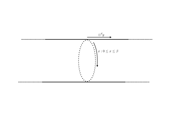
Figure 1: An infinite cylinder in $D=d+1$ spacetime dimensions. For the thermal channel, $x$ is euclidean time and $y$ refers to $d$ spatial directions. For the SpC channel $x$ is a single compactified spatial coordinate and one $y$ coordinate is time $-\infty<t<\infty$.

Thermal channel.    If the compactified direction is euclidean time, then this is interpreted as the QFT at finite temperature $T=1/\beta$. In this picture the Hilbert space corresponds to particles of arbitrary continuous momentum ${\bf{k}}$ in $d$ spatial dimensions. We will refer to this as the Thermal channel.

Spatially compactified channel. The compactified direction can be viewed as a spatial coordinate. For $D=2$, one would say the hamiltonian “lives” on the circle, i.e. the Hilbert space is the quantized states on a circle, and the other direction corresponds to time evolution. In this case, one component of the spatial momenta are not continuous but quantized. We will refer to this as the SpC  channel.

As we will see below even for free QFT’s, the Thermal channel has several advantages. One is that the integrals involved are convergent if the theory is UV complete. On the other hand, the SpC channel requires a detailed regularization that in principle makes it non-universal. As discussed below Modularity can serve as a constraint for the regularization procedure.

III.2 Thermodynamic definition of ${\rho_{\rm vac}}$

Let us first consider the Thermal channel. As usual we define the partition function and free energy density ${\cal F}$,

$$Z={\rm Tr}\,e^{-\beta H},~{}~{}~{}~{}~{}{\cal F}=-\dfrac{1}{\beta{\cal V}}\log Z$$ (9)

where ${\cal V}$ is the $d$ dimensional uncompactified spatial volume. The energy density and pressure are given by

$$\rho=\partial_{\beta}\left(\beta{\cal F}\right),~{}~{}~{}~{}~{}p=-{\cal F}$$ (10)

and the entropy density is

$${\cal S}=\beta^{2}\,\dfrac{\partial{\cal F}}{\partial\beta}=\beta\,(\rho+p).$$ (11)

Let us assume that there is a single fundamental mass scale $m$ such that all physical masses are proportional to $m$. The Standard Model of particle physics is such a model if one accepts that all fundamental masses arise from spontaneous symmetry breaking in the Higgs sector. String Theory is also a theory with a single mass scale. Then it is convenient to define the scaling function $c(r)$:

$${\cal F}=-\dfrac{\chi(D)}{\beta^{D}}\,\,c(r),~{}~{}~{}~{}~{}r\equiv m\beta,~{}~{}~{}~{}~{}\chi(D)\equiv\pi^{-D/2}\Gamma(D/2)\zeta(D).$$ (12)

The function $\chi(z)$ satisfies the functional equation

$$\chi(z)=\chi(1-z)$$ (13)

in the entire complex plane (except at the pole at $z=1$), as first discovered by Riemann. This functional equation will be be crucial to Modularity discussed below. The normalization in (12) is such that for a free massless boson, $\lim_{r\to 0}c(r)=c_{\rm uv}=1$ independent of $r$. For $D=2$ unitary theories, $c_{\rm uv}$ is the Virasoro central charge.

For unitary theories in 2D, the c-theorem implies $c(r)$ decreases with $r$ctheorem . For our thermodynamic definition of $c(r)$,

$$\partial_{r}c(r)<0~{}~{}~{}~{}~{}~{}~{}\Longrightarrow~{}~{}\rho>(D-1)p.$$ (14)

For the free massive free theories considered below, this condition is satisfied. As we will see below it is also satisfied for QCD (See Figure 4.) It would be nice to show that $c(r)$ decreases based on general principles, however this is beyond the scope of the present article.

If the QFT is UV complete, then there should be a power series expansion in $r$:

$$\lim_{r\to 0}\,c(r)=c_{\rm uv}+\sum_{\mathfrak{p}>0}c_{\mathfrak{p}}\,r^{\mathfrak{p}}$$ (15)

where $\mathfrak{p}$ denotes certain powers. These powers are not necessarily integers, but can depend on the anomalous scaling dimension of relevant operators in the UV. Also as we will see, some powers have $\log r$ corrections.

Definition of ${\rho_{\rm vac}}$.     Vacuum energy with $p=-\rho$ would correspond to $\partial_{\beta}{\cal F}=0$ based on (10), and this is not satisfied for arbitrary ${\cal F}(\beta)$ as expected. However if $c(r)\sim r^{D}$ then $\partial_{\beta}{\cal F}=0$. We thus identify ${\rho_{\rm vac}}$ with the $c_{\scriptscriptstyle{D}}$ term:

$$c_{\rm vac}(r)=c_{\scriptscriptstyle{D}}r^{D},$$ (16)

where $c_{{\scriptscriptstyle{D}}}$ is a constant. This leads to the definition

$${\rho_{\rm vac}}=-c_{{\scriptscriptstyle{D}}}\,\chi(D)\,m^{D}.$$ (17)

Since $r\to 0$ corresponds to $\beta\to 0$ for fixed $m$, the above ${\rho_{\rm vac}}$ is effectively calculated in the UV since it corresponds to the limit of infinite temperature.

Now consider the SpC channel. Here $\beta$ is not interpreted as a temperature but rather a finite spatial size. Formally one has

$${\cal F}=\langle{\rm vac;\beta}|\,H|{\rm vac;\beta}\rangle$$ (18)

where $|{\rm vac;\beta}\rangle$ is a complicated $\beta$-dependent vacuum. As we will see, computations in this channel are more complicated than for the Thermal channel since it requires some subtle regularization of divergences.

III.3 Required properties of ${\rho_{\rm vac}}$

In this section we list several properties of ${\rho_{\rm vac}}$ we require to be valid, as they will serve as non-trivial checks of our proposal.

Property 1.

We assume that the QFT is UV complete such that the power series (15) is well-defined.

Property 2.

If the QFT is conformally invariant, i.e. a CFT, then ${\rho_{\rm vac}}=0$. The reason is simple: the CFT only has the leading $c_{\rm uv}$ term in the expansion (15). This implies free massless particles have ${\rho_{\rm vac}}=0$.

Property 3.

The entropy associated with the vacuum state is zero. This is evident from (11) with $p=-\rho$.

Property 4.

Bose-Fermi symmetry. Introduce a statistical parameter $s$, where $s=1,-1$ corresponds to bosons, fermions respectively. For the complete ${\cal F}(r)$ there is no Bose-Fermi symmetry for a particle of a fixed mass since there is no such symmetry between the Bose-Einstein (BE) and Fermi-Dirac (FD) distributions. However for the term that defines ${\rho_{\rm vac}}$, we expect that bosons and fermions contribute with opposite signs, namely ${\rho_{\rm vac}}\propto s$. The arguments are simple and well-known, nevertheless we repeat them here, in part since we wish to present an analogous result for interacting theories.

Consider the action for a single bosonic field $\phi$ in zero spatial dimensions:

$$S=\int dt\left(\dfrac{1}{2}\partial_{t}\phi\partial_{t}\phi-\dfrac{\omega^{2}}{2}\phi^{2}\right)$$ (19)

The equation of motion is $\partial_{t}^{2}\phi=-\omega^{2}\phi$, thus $\phi$ can be expanded as follows: $\phi=\left(ae^{-i\omega t}+a^{\dagger}e^{i\omega t}\right)/\sqrt{2\omega}$. Canonical quantization gives $[a,a^{\dagger}]=1$, and the hamiltonian is

$$H=\dfrac{1}{2}\left(\partial_{t}\phi\partial_{t}\phi+\omega^{2}\phi^{2}\right)=\dfrac{\omega}{2}(aa^{\dagger}+a^{\dagger}a)=\omega(a^{\dagger}a+\dfrac{1}{2})$$ (20)

The zero-point energy is identified as $\omega/2$.

For fermions, the zero point energy has the opposite sign. To see this, consider a zero dimensional version of a Majorana fermion with action

$$S=\int dt\left(i\overline{\psi}\partial_{t}\overline{\psi}-i\psi\partial_{t}\psi-\omega\overline{\psi}\psi\right)$$ (21)

The equation of motion is $\partial_{t}\psi=-i\omega\overline{\psi}$, and $\partial_{t}\overline{\psi}=-i\omega\psi$, and thus $\psi,\overline{\psi}$ have the following expansion: $\psi=\dfrac{1}{\sqrt{2}}\left(be^{i\omega t}+b^{\dagger}e^{-i\omega t}\right)$, and $\overline{\psi}=\dfrac{1}{\sqrt{2}}\left(-be^{i\omega t}+b^{\dagger}e^{-i\omega t}\right)$. Canonical quantization leads to $\{b,b^{\dagger}\}=1,b^{2}={b^{\dagger}}^{2}=0$, and the hamiltonian is

$$H=\omega\overline{\psi}\psi=\dfrac{\omega}{2}\left(b^{\dagger}b-bb^{\dagger}\right)=\omega(b^{\dagger}b-\dfrac{1}{2})$$ (22)

and the zero point energy is $-\omega/2$.

For non-free theories, this property also follows trivially from supersymmetry . It is well-known that a finite temperature breaks supersymmetry, for the simple reason that there is no such symmetry between the BE and FD distributions Grisaru . However a simple argument shows that supersymmetry implies that ${\rho_{\rm vac}}=0$. Let $Q$ be a conserved supercharge where schematically $Q^{2}=H$. If $Q|{\rm vac}\rangle=0$, then $\langle{\rm vac}|H|{\rm vac}\rangle=0$, implying that bosons and fermions have zero point energies of opposite sign, and ${\rho_{\rm vac}}=0$.

Let us also mention a generalization that is realized in $2D$. Suppose the hamiltonian $H$ is in the center of the universal enveloping algebra of some conserved charges $Q$. For instance the sine-Gordon model at certain rational points of the coupling constant has conserved charges satisfying $Q^{p}=H$ where $p$ is an even integer Vafa . Then by the same argument, if $Q|{\rm vac}\rangle=0$ then ${\rho_{\rm vac}}=0$. We will confirm this below when we consider ${\rho_{\rm vac}}$ for the sine-Gordon model.

Property 5.

Modularity.    Deceptively simple as it may appear, calculations of ${\rho_{\rm vac}}$ in the Thermal and SpC channels must agree. As we will show below, this is rather non-trivial since the calculations are completely different. In these computations, Riemann’s functional equation (13) is crucial.

For a $2D$ conformal field theory, one can impose boundary conditions on our infinite cylinder such that it is a torus. Here the partition function enjoys the full $SL(2,\mathbb{Z})$ modular invariance Cardy . A subgroup of the modular group simply exchanges the two cycles, i.e. exchanges space and time, which is the distinction between the Thermal and SpC channels. For non-conformal theories in arbitrary dimensions we expect the latter to hold not only for ${\rho_{\rm vac}}$ but for the entire ${\cal F}$, and will refer to it as Modularity.

Property 6.

For this article, we don’t implicitly assume nor consider spontaneous symmetry breaking (SSB). We will see that in QCD for instance, one does not need to assume SSB to compute ${\rho_{\rm vac}}$. We should also mention that examples with SSB of supersymmetry were already considered in Mingling .

IV The massive free field case in $D$ spacetime dimensions

IV.1 The naive computation that leads to a discrepancy by $10^{120}$ orders of magnitude

Although this computation should be obsolete by now, we present it here since the discrepancy by a factor of $10^{120}$ is still often quoted in the literature. It will also serve as a point of comparison with a properly regularized definition below. Consider a free massive bosonic or fermionic field, which can be viewed as an infinite collection of harmonic oscillators with zero point energy $\sqrt{{\bf{k}}^{2}+m^{2}}$:

$$\rho_{\rm vac,cutoff}=\dfrac{s}{2}\int_{|{\bf{k}}|\leq{k_{c}}}\dfrac{d^{d}{\bf{k}}}{(2\pi)^{d}}\,\sqrt{{\bf{k}}^{2}+m^{2}}.$$ (23)

There is already one problem in that if one naively computes the pressure using a similar expression, it does not satisfy $p=-\rho$ Martin . Using

$$\int\dfrac{d^{d}{\bf{k}}}{(2\pi)^{d}}=\Omega_{d}\int k^{d-1}dk,~{}~{}~{}~{}~{}~{}\Omega_{d}=\dfrac{1}{\Gamma(\tfrac{d}{2})2^{d-1}\pi^{d/2}}~{}~{}~{}~{}~{}~{}k=|{\bf{k}}|$$ (24)

the integral can be performed for arbitrary $d$ and expressed in terms of a hyper-geometric function:

$$\rho_{\rm vac,cutoff}=s\,\left(\dfrac{m\,{k_{c}}^{d}}{2d}\right)\,\Omega_{d}~{}_{2}F_{1}\left[-\tfrac{1}{2},\tfrac{d}{2},\tfrac{2+d}{2},-\tfrac{{k_{c}}^{2}}{m^{2}}\right].$$ (25)

For our purposes it is more useful to consider each integer spacetime dimension $D$ separately. For ${k_{c}}\gg m$ one finds

$$\rho_{\rm vac,cutoff}=s\begin{cases}\dfrac{{k_{c}}^{2}}{4\pi}+\dfrac{m^{2}}{4\pi}\,\log(2{k_{c}}/m)~{}~{}~{}~{}~{}~{}~{}~{}~{}(D=2)\\ \\ \dfrac{{k_{c}}^{3}}{12\pi}-\dfrac{m^{3}}{12\pi}~{}~{}~{}~{}~{}~{}~{}~{}~{}~{}~{}~{}~{}~{}~{}~{}~{}~{}~{}~{}~{}~{}~{}(D=3)\\ \\ \dfrac{{k_{c}}^{4}}{16\pi^{2}}-\dfrac{m^{4}}{32\pi^{2}}\,\log(2{k_{c}}/m)~{}~{}~{}~{}~{}(D=4)\end{cases}$$ (26)

The $120$ orders of magnitude arises when one chooses the cut-off ${k_{c}}$ to be the Planck scale and compares with the measured value (5). Note the $\log$ corrections in even dimensions, which will reappear below with a proper regularization that removes the cut-off dependence. Note also the difference in signs for $D=2$ verses $D=4$.

IV.2 Thermal Channel

We begin with a standard result from quantum statistical mechanics:

$${\cal F}=\dfrac{s}{\beta}\int\dfrac{d^{d}{\bf{k}}}{(2\pi)^{d}}\,\log\left(1-s\,e^{-\beta\,\omega_{\bf{k}}}\right),~{}~{}~{}~{}~{}\omega_{k}=\sqrt{{\bf{k}}^{2}+m^{2}}$$ (27)

An important advantage of the Thermal channel is that the above integrals are already convergent. It remains to extract $c_{\rm vac}(r)$ from it. Rescaling ${\bf{k}}\to 2\pi{\bf{k}}/\beta$

$${\cal F}=\dfrac{s}{\beta^{d+1}}\Omega_{d}\,\int_{0}^{\infty}dkk^{d-1}\log\left(1-s\,e^{-\,\sqrt{k^{2}+r^{2}}}\right),~{}~{}~{}~{}~{}r=m\beta.$$ (28)

Expanding out the $\log$, the scaling function $c(r)$ can then be expressed

$$c(r)=\dfrac{r^{{\scriptscriptstyle{D}}/2}\pi^{-{\scriptscriptstyle{D}}/2}}{2^{({\scriptscriptstyle{D}}-2)/2}\,\chi({\scriptscriptstyle{D}})}\,\sum_{n=1}^{\infty}\dfrac{s^{n+1}}{n^{{\scriptscriptstyle{D}}/2}}\,K_{\tfrac{{\scriptscriptstyle{D}}}{2}}(nr)$$ (29)

where $K_{\nu}(z)$ is the modified Bessel function. Using the expansion

$$\lim_{r\to 0}K_{\tfrac{{\scriptscriptstyle{D}}}{2}}(nr)=r^{-{\scriptscriptstyle{D}}/2}\,2^{({\scriptscriptstyle{D}}-2)/2}\,n^{-{\scriptscriptstyle{D}}/2}\,\Gamma(\tfrac{{\scriptscriptstyle{D}}}{2})+{\cal O}(r^{{\scriptscriptstyle{D}}/2}),$$ (30)

and the following property of the Riemann zeta function

$$\zeta(z)=\sum_{n=1}^{\infty}\dfrac{1}{n^{z}}=(1-\dfrac{1}{2^{z-1}})^{-1}\,\sum_{n=1}^{\infty}\dfrac{(-1)^{n+1}}{n^{z}},~{}~{}~{}~{}~{}\Re(z)>1,$$ (31)

one can easily show that the leading term is

$$\lim_{r\to 0}c(r)=c_{\rm uv}=\begin{cases}1,~{}~{}{~{}~{}~{}~{}~{}~{}~{}~{}~{}~{}~{}\rm for~{}bosons}~{}~{}~{}(s=1)\\ 1-\dfrac{1}{2^{{\scriptscriptstyle{D}}-1}},~{}~{}{\rm for~{}fermions}~{}(s=-1).\end{cases}$$ (32)

We now turn to the small $r$ corrections in order to determine ${\rho_{\rm vac}}$. As we will see, each spacetime dimension $D$ should be treated separately.

IV.2.1 $D=2$

This case was studied to all orders in $r$ by Mussardo in his book MussardoBook . In fact there Modularity was established to all orders.

For our purposes of computing the $c_{\rm vac}(r)\propto r^{2}$ term we carry out the calculation in a somewhat simpler but similar fashion. As for the TBA we consider

$$\dfrac{1}{r}\partial_{r}c(r)=-\dfrac{1}{\zeta(2)}\sum_{n=1}^{\infty}s^{n+1}\,K_{0}(nr),$$ (33)

where

$$K_{0}(nr)=-\left(\log r+\log n-\log 2+\gamma_{E}\right)+{\cal O}(r^{2}).$$ (34)

One encounters the following sum which we regulate with the zeta function:

$$\sum_{n=1}^{\infty}s^{n+1}\doteq s\,\zeta(0)=-s/2,$$ (35)

where the symbol $\doteq$ denotes regularization based on the $\zeta(z)$ function. One also encounters the sum $\sum_{n=1}^{\infty}s^{n+1}\,\log n$. Using

$$\sum_{n=1}^{\infty}\dfrac{s^{n+1}}{n^{\epsilon}}=\sum_{n+1}^{\infty}s^{n+1}\,e^{-\epsilon\log n},$$ (36)

one regulates this as

$$\sum_{n=1}^{\infty}s^{n+1}\,\log n~{}\doteq-s\,\zeta^{\prime}(0)=\dfrac{s}{2}\log 2\pi,$$ (37)

where $\zeta^{\prime}(z)=\partial_{z}\zeta(z)$. Integrating over $r$ one obtains

$$c(r)=c_{\rm uv}+\dfrac{3r^{2}s}{2\pi^{2}}\left(\log(4\pi/r)+\tfrac{1}{2}-\gamma_{E}\right)+{\cal O}(r^{4}),$$ (38)

where $\gamma_{E}=0.5772..$ is the Euler-Mascheroni constant. From equation (17) one finally obtains

$${\rho_{\rm vac}}=-s\,\dfrac{m^{2}}{4\pi}\left(\log(4\pi/r)+\tfrac{1}{2}-\gamma_{E}\right).$$ (39)

IV.2.2 $D=3$

This case has some new features in comparison with $2D$. Begin with

$$c(r)=\sqrt{\dfrac{2}{\pi}}\,\left(\dfrac{r^{3/2}}{\zeta(3)}\right)\sum_{n=1}^{\infty}\dfrac{s^{n+1}}{n^{3/2}}\,K_{\tfrac{3}{2}}(nr)$$ (40)

For half-integers $\nu$, $K_{\nu}(z)$ has simple expressions:

$$K_{\tfrac{3}{2}}(nr)=\sqrt{\dfrac{\pi}{2}}\,e^{-nr}\,r^{-3/2}\,\left(\dfrac{1+nr}{n^{3/2}}\right),$$ (41)

which leads to the exact formula

$$c(r)=\dfrac{s}{\zeta(3)}\left[{\rm Li}_{3}(s\,e^{-r})+r\,{\rm Li}_{2}(s\,e^{-r})\right],$$ (42)

where ${\rm Li}_{z}(x)=\sum_{n=1}^{\infty}\,x^{n}/n^{z}$ is a poly-logarithm. Expanding the poly-log in powers of $r$:

$$\lim_{r\to 0}c(r)=c_{\rm uv}+\dfrac{1}{\zeta(3)}\left[\dfrac{s\log(1-s)}{2}\,r^{2}+\dfrac{r^{3}}{3(1-s)}\right]+{\cal O}(r^{4}).$$ (43)

Note that there is no $\log r$ term in comparison with $2D$. However one needs to regularize the singular $s$ dependence for $s=1$, and we do this again by analytic continuation of $\zeta(z)$. Using (35)

$$\dfrac{1}{1-s}=\sum_{n=1}^{\infty}s^{n+1}\,\doteq-s/2.$$ (44)

Expanding $\log(1-s)$ and using (35)

$$\log(1-s)\doteq\dfrac{1}{4}.$$ (45)

Putting all this together one obtains

$$c(r)=c_{\rm uv}+\dfrac{s\,r^{2}}{8\zeta(3)}-\dfrac{s\,r^{3}}{6\zeta(3)}+{\cal O}(r^{4}).$$ (46)

Based on (17) one then finds the simple result

$${\rho_{\rm vac}}=s\,\dfrac{m^{3}}{12\pi}.$$ (47)

Note that it satisfies the Bose-Fermi Property 3.

IV.2.3 $D=4$

Here

$$c(r)=-\dfrac{\pi^{2}\beta^{4}}{\zeta(4)}\,{\cal F}.$$ (48)

The calculation is similar to the $2D$ case. To simplify it we just deal with $c(r)$ directly rather than $\partial_{r}c(r)$:

$$c(r)=\dfrac{45\,r^{2}}{\pi^{4}}\sum_{n=1}^{\infty}\dfrac{s^{n+1}}{n^{2}}\,K_{2}(nr)$$ (49)

Expanding the Bessel function

$$K_{2}(nr)=\left(\dfrac{2}{n^{2}r^{2}}-\dfrac{1}{2}\right)+\dfrac{r^{2}n^{2}}{32}\left(3-4\gamma_{E}-4\log(nr/2)\right)+{\cal O}(r^{4}).$$ (50)

Regularizing sums involving the statistical parameter $s$ as above, one obtains

$$c(r)=c_{\rm uv}-\dfrac{15r^{2}}{16\pi^{2}}(3+s)-\dfrac{45\,s\,r^{4}}{16\pi^{4}}\left(\log(4\pi/r)+\tfrac{3}{4}\ -\gamma_{E}\right)+{\cal O}(r^{6}).$$ (51)

This leads to

$${\rho_{\rm vac}}=s\,\dfrac{m^{4}}{32\pi^{2}}\left(\log(4\pi/r)+\tfrac{3}{4}-\gamma_{E}\right),$$ (52)

Note that the $r^{2}$ term in $c(r)$ is not proportional to $s$ as expected due to the asymmetry between BE and FD distributions. However the $r^{4}$ term which determines ${\rho_{\rm vac}}$ is indeed consistent with Bose-Fermi symmetry Property 3.

Remark.    Note that for all $3$ cases of $D$, ${\rho_{\rm vac}}$ has the opposite sign to the cut-off expressions (26), which is presumably due to the subtraction of divergent terms as ${k_{c}}\to\infty$. It is also interesting that up to this sign, the $\log$ terms in even dimensions follows simply by replacing the cut-off ${k_{c}}\to 2/\beta$ which is consistent with the fact that $\beta\to 0$ is the UV limit.

IV.3 Spatially compactified channel: Modularity

The SpC channel is essentially the same as for the naive calculation in Section IVA, however regularized with $\beta$. Calculations in the SpC channel are more difficult for at least two reasons. First is that UV divergences are severe. Riemann’s functional identity (13) will play a central role in regulating these divergences. Secondly, the statistical parameter $s$ is not simply a parameter as in the Thermal channel, such that bosons and fermions have to be treated separately. Given these significant differences, we carry out calculations of ${\rho_{\rm vac}}$ in this channel as a check of Modularity, Principle 4. This also serves as a check of Bose-Fermi symmetry, Principle 3.

For arbitrary $D=d+1$, we begin with

$${\cal F}_{\rm sum}=\dfrac{s}{2\beta}\sum_{n}\int\dfrac{d^{d-1}{\bf{k}}}{(2\pi)^{d-1}}~{}\sqrt{{\bf{k}}^{2}+\left(\dfrac{2\pi n}{\beta}\right)^{2}+m^{2}},~{}~{}~{}~{}~{}~{}~{}{\rm where}~{}\begin{cases}~{}~{}~{}~{}~{}n\in\mathbb{Z}~{}{\rm for}~{}{\rm bosons}~{}(s=1)\\ n\in\mathbb{Z}+\tfrac{1}{2}~{}{\rm for}~{}{\rm fermions}(s=-1).\end{cases}$$ (53)

We require that as for the Thermal channel, in the infra-red (IR) $\lim_{r\to\infty}{\cal F}(r)\to 0$. More generally this is a consequence of a massive theory where the infra-red limit of the QFT is empty since all masses are going to infinity in this limit, i.e. $\lim_{r\to\infty}c(r)=0$. This also implies the entropy density ${\cal S}$ in (11) is zero in this limit, as it should be. It is implicit in this condition that the theory does not have a non-trivial IR fixed point CFT, which is of course known to be the case for free massive QFT’s.

Following Mussardo MussardoBook , we deal with this with the subtraction:

$${\cal F} = {\cal F}_{\rm sum}-{\cal F}_{\rm int}$$ (54)

$${\cal F}_{\rm int} = \dfrac{s}{2\beta}\int_{-\infty}^{\infty}dx\int\dfrac{d^{d-1}{\bf{k}}}{(2\pi)^{d-1}}\sqrt{{\bf{k}}^{2}+\left(\dfrac{2\pi x}{\beta}\right)^{2}+m^{2}}.$$ (55)

The above expression for ${\cal F}$ still has UV divergences, however as we will see, they are more easily interpreted.

We present calculations for $D=2$ bosons and fermions in more detail since similar details appear for $D=4$. We leave the general case of $D=3$ bosons and fermions, and $D=4$ fermions as an exercise.

IV.3.1 D=2 Bosons

Here the single spatial momentum ${\bf{k}}$ is quantized and there are no leftover spatial integrals:

$${\cal F}_{\rm sum}=\dfrac{1}{2\beta}\sum_{n\in\mathbb{Z}}\sqrt{m^{2}+\left(\dfrac{2\pi n}{\beta}\right)^{2}}$$ (56)

Expanding out the square root in powers of $r=m\beta$,

$${\cal F}_{\rm sum}=\dfrac{\pi}{\beta^{2}}\sum_{n\in\mathbb{Z}}\sqrt{n^{2}+\dfrac{r^{2}}{4\pi^{2}}}=\dfrac{\pi}{\beta^{2}}\sum_{n\in\mathbb{Z}}\left(|n|+\dfrac{r^{2}}{8\pi^{2}\,|n|}\right)+{\cal O}(r^{4})$$ (57)

For $\zeta(z)$ with $z\neq 1$, one can rely on analytic continuation:

$$\sum_{n\in\mathbb{Z}}|n|=2\,\zeta(-1)=-\tfrac{1}{6}.$$ (58)

On the other hand, the other sum cannot be dealt with this way because of the pole in $\zeta(z)$ at $z=1$. Indeed one encounters a singularity due to the zero mode $n=0$:

$$\sum_{n\in\mathbb{Z}}\dfrac{1}{|n|}=2\,\zeta(1)+\tfrac{1}{0}.$$ (59)

We discard this $\tfrac{1}{0}$ singularity, since as we will see this is needed to satisfy the Bose-Fermi Property 3, as there is no zero mode for fermions. Leaving the singular $\zeta(1)$ as unevaluated for the moment, in summary we have

$${\cal F}_{\rm sum}=-\dfrac{\pi}{12\beta^{2}}+\dfrac{r^{2}}{4\pi\beta^{2}}\,\zeta(1)+{\cal O}(r^{4}).$$ (60)

Next we turn to ${\cal F}_{\rm int}$. The integral over $x$ is still divergent, thus we introduce a cut-off ${N_{c}}$ in the integral over $x$:

$${\cal F}_{\rm int}=-\dfrac{2\pi}{\beta^{2}}\,\int_{0}^{N_{c}}dx\,\sqrt{x^{2}+(r/2\pi)^{2}}.$$ (61)

Expanding out the square-root,

$${\cal F}_{\rm int}=\dfrac{\pi}{\beta^{2}}\left({N_{c}}^{2}+\dfrac{r^{2}}{4\pi^{2}}\left(\log(4\pi/r)+\log{N_{c}}+\tfrac{1}{2}\right)\right)+\ldots$$ (62)

We now regularize $\zeta(1)$ in (60) in a way that is equivalent to the $N_{c}$ regularization of ${\cal F}_{\rm int}$. Using the harmonic number:

$$\zeta_{c}(1)=\sum_{n=1}^{N_{c}}\dfrac{1}{n}=\log{N_{c}}+\gamma_{E}+\ldots$$ (63)

Putting this all together, the $\log N_{c}$ cancels and one reproduces equations (38) and (39) for $s=1$.

IV.3.2 D=2 fermions

Here the calculation nearly identical, except for the sums over $n$ half-integer. This implies there is no zero mode $n=0$ to deal with. The sums over $n$ can be dealt with using the Hurwitz $\zeta$ function

$$\zeta(z,a)=\sum_{n=0}^{\infty}\dfrac{1}{(n+a)^{z}},$$ (64)

which satisfies

$$\zeta(z,\tfrac{1}{2})=(2^{z}-1)\zeta(z).$$ (65)

This leads to

$$\sum_{n\in\mathbb{Z}+\tfrac{1}{2}}|n| = 2\,\zeta(-1,\tfrac{1}{2})=\tfrac{1}{12}$$ (66)

$$\sum_{n\in\mathbb{Z}+\tfrac{1}{2}}\dfrac{1}{|n|} = 2\,\zeta(1,\tfrac{1}{2})=2\,\zeta(1).$$ (67)

Repeating arguments for the $2D$ boson case in the last sub-section, the final result again agrees with equations (38),(39), in this case for $s=-1$.

IV.3.3 D=4 bosons

In this case there are two one leftover spatial ${\bf{k}}$ integrals. Again rescaling ${\bf{k}}\to 2\pi{\bf{k}}/\beta$ one obtains

$${\cal F}_{\rm sum}=\dfrac{2\pi^{2}}{\beta^{4}}\sum_{n\in\mathbb{Z}}\int_{0}^{k_{c}}dk\,k\,\sqrt{n^{2}+k^{2}+\dfrac{r^{2}}{4\pi^{2}}}.$$ (68)

The integral over $k$ is simpler if one considers $\partial_{r}{\cal F}$. Dropping all $k_{c}$ dependence as ${k_{c}}\to\infty$ one has

$$\partial_{r}{\cal F}_{\rm sum}=-\dfrac{r}{2\beta^{4}}\sum_{n\in\mathbb{Z}}\sqrt{n^{2}+\left(\dfrac{r}{2\pi}\right)^{2}}.$$ (69)

Expanding the square-root,

$$\partial_{r}{\cal F}_{\rm sum}=-\dfrac{2\pi}{\beta^{4}}\left(\dfrac{r}{2\pi}\,\zeta(-1)+\dfrac{r^{3}}{16\pi^{3}}\zeta(1)\right)+{\cal O}(r^{3}),$$ (70)

and integrating this equation one finds

$${\cal F}_{\rm sum}(r)-{\cal F}_{\rm sum}(0)=-\dfrac{1}{2\beta^{4}}\left(r^{2}\zeta(-1)+\dfrac{r^{4}}{16\pi^{2}}\zeta(1)\right)+{\cal O}(r^{6}).$$ (71)

The leading $r=0$ term is

$${\cal F}_{\rm sum}(r=0)=-\dfrac{4\pi^{2}}{3\beta^{4}}\zeta(-3)$$ (72)

which leads to $c_{\rm uv}=4\pi^{4}\zeta(-3)/3\zeta(4)=1$, as expected.

Next consider ${\cal F}_{\rm int}$. Using essentially the same arguments as for $D=2$, one finds

$$\partial_{r}{\cal F}_{\rm int}=-\dfrac{r^{3}}{8\pi^{2}\beta^{4}}\left(\log\left(4\pi/r\right)+\log{N_{c}}+\tfrac{1}{2}\right).$$ (73)

Integrating this equation:

$${\cal F}_{\rm int}=-\dfrac{r^{4}}{32\pi^{2}\beta^{4}}\left(\log\left(4\pi/r\right)+\log{N_{c}}+\tfrac{3}{4}\right)+\ldots$$ (74)

One can easily check that ${\cal F}={\cal F}_{\rm sum}-{\cal F}_{\rm int}$ gives the same result as equations (51), (52) for $s=1$, hence establishing modularity in this $D=4$ bosonic case.

V Integrable theories in $D=2$

There are many integrable QFT’s in $D=2$ spacetime dimensions available for exploring the above ideas, and can be useful for further developing them. These integrable QFT’s are characterized by a factorizable S-matrix, and the exact free energy density, and thus $c(r)$, can be computed exactly in the Thermal channel from the TBA, which involves a complicated integral equation. The term $c_{\rm vac}(r)\propto r^{2}$ which determines ${\rho_{\rm vac}}$ is commonly referred to as the “bulk” term $c_{\rm bulk}$. For diagonal scattering, namely where scattering of particles of type $a$ and $b$ produces particles of the same type, there exists a universal formula for $c_{\rm vac}$ due to Al. Zamolodchikov ZamoTBA . Very interestingly, ${\rho_{\rm vac}}$ depends only on physical S-matrix parameters of the scattering of the lightest particle with itself and the scale of ${\rho_{\rm vac}}$ is set by the physical mass of this lightest particle. Since the S-matrices can be bootstrapped starting with the lightest particle, we henceforth refer to this property as the Lightest Mass Bootstrap (LMB) property. Destri and deVega obtained the same result in the Toda example below in a very different manner that is closer to the SpC channel DestriDeVega ; we will return to discussing the latter work below.

One subtlety must be kept in mind while interpreting the results. In 2D the notion of whether a physical particle is a boson or fermion is blurred since there is no spin-statistics theorem. In particular, the TBA equations are necessarily of fermionic type, otherwise the solutions are not well-defined in the UV MussardoSimon . In the S-matrix description, the statistical parameter $s=\pm 1$ is defined as

$$\lim_{\theta\to 0}S(\theta)=s$$ (75)

where $\theta$ is the rapidity, $E=m\cosh\theta,~{}p=m\sinh\theta$, and for all physical theories with non-trivial S-matrix, $s=-1$.

We first consider the sine-Gordon model which has a rich spectrum of particles. We considered this case already in Mingling , however we repeat some of this here in order to make some additional observations. As we will see, ${\rho_{\rm vac}}$ satisfies Property 3 at certain (fractional) supersymmetric points. It will also be interesting to observe how ${\rho_{\rm vac}}$ behaves near the marginal point.

The second example is a model of multiple scalar fields, the affine Toda theories, where each field leads to a physical particle of a given mass. We will show how the exact result at weak coupling can be derived in a semi-classical analysis. This example may serve as a tool to understand ${\rho_{\rm vac}}$ using ordinary perturbation theory in a way that may lead to insights in higher dimensions, however this is not pursued here.

V.1 Exact formula for ${\rho_{\rm vac}}$

Let us present the general formula for ${\rho_{\rm vac}}$ for theories with diagonal scattering ZamoTBA ; KlassenMelzer and explain the LMB property in this context. The basic building blocks of the two-body S-matrices $S(\theta)$ are factors of $f_{\alpha}(\theta)$:

$$S(\theta)=\prod_{\alpha\in{\cal A}}f_{\alpha}(\theta),~{}~{}~{}~{}~{}f_{\alpha}(\theta)\equiv\dfrac{\sinh\tfrac{1}{2}\left(\theta+i\pi\alpha\right)}{\sinh\tfrac{1}{2}\left(\theta-i\pi\alpha\right)},$$ (76)

and ${\cal A}$ is a finite set of $\alpha$’s. The angles $\pi\alpha$ correspond to resonance poles in the complex $\theta$ plane for the S-matrices.

Suppose the theory consists of many particles with masses $m_{a},~{}{a=1,2,\ldots}$, where $m_{1}$ is the lightest particle, and the S-matrix for the scattering of $m_{1}$ with itself is $S_{11}(\theta)$ of the form (76). Then one has the simple formula

$$c_{\rm vac}=-\dfrac{3r^{2}}{\pi\mathfrak{g}},~{}~{}~{}~{}~{}~{}r=m_{1}\beta,~{}~{}~{}~{}~{}\mathfrak{g}=2\sum_{\alpha\in{\cal A}}\sin\pi\alpha.$$ (77)

Finally (17) gives

$${\rho_{\rm vac}}=\dfrac{m_{1}^{2}}{2\mathfrak{g}}.$$ (78)

V.2 sine-Gordon/massive Thirring model

The sine-Gordon theory can be defined by the following action for a single scalar field:

$${\cal S}=\int d^{2}x\left(\dfrac{1}{8\pi}(\partial_{\mu}\phi\,\partial^{\mu}\phi)+2\mu\cos(\sqrt{2}\,\widehat{\beta}\phi)\right).$$ (79)

The cosine term has scaling dimension $\Gamma_{\rm uv}=2\widehat{\beta}^{2}$, thus it is relevant for $0<\widehat{\beta}^{2}<1$. This unitary theory has a UV completion which is just a free boson with $c_{\rm uv}=1$. In is equivalent to the massive Thirring model with action Coleman

$${\cal S}=\int d^{2}x\left(i\overline{\psi}\gamma^{\mu}\partial_{\mu}\psi-m\overline{\psi}\psi-\tfrac{g}{2}(\overline{\psi}\gamma^{\mu}\psi)^{2}\right),~{}~{}~{}~{}~{}~{}g=\pi\left(1/{(2\widehat{\beta}^{2})}-1\right).$$ (80)

The charged solitons of the sine-Gordon model correspond to the Thirring fermion. The free fermion point occurs at $\widehat{\beta}^{2}=1/2$. For $\widehat{\beta}^{2}<1/2$ there is a rich spectrum of bound states of the fermion and the complete S-matrix was found in ZamoZamo0 , with the help of the Yang-Baxter equation.

For generic $\widehat{\beta}$, the scattering is non-diagonal. However at the couplings $\widehat{\beta}^{2}=1/j,~{}~{}~{}~{}{\rm for}~{}~{}j=2,3,\ldots$ then there are $j-2$ breathers and the scattering is diagonal. These points are referred to as “reflectionless” due to the diagonal scattering. The soliton is obviously the lightest mass particle. Letting $s,\overline{s}$ denote the soliton, anti-soliton, it’s S-matrix is well-known ZamoZamo0 :

$$S_{s\overline{s}}=\prod_{k=1}^{j-2}f_{k/(j-1)}(\theta).$$ (81)

This gives $\mathfrak{g}=2\sum_{k=1}^{j-2}\sin(\pi k/(j-1))=2\cot(\pi/(2j-2))$. Expressing $j$ in terms of $\widehat{\beta}$, then at the reflectionless points

$${\rho_{\rm vac}}=\dfrac{m_{s}^{2}}{4}\,\tan\left(\dfrac{\pi\widehat{\beta}^{2}}{2(1-\widehat{\beta}^{2})}\right).$$ (82)

It was argued that we can analytically continue the above formula to $\widehat{\beta}^{2}>1/2$, where there are only solitons in the spectrum.

The above formula has several very interesting and illustrative features. See Figure 2.

$\bullet$   For generic irrational $0<\widehat{\beta}^{2}<1$, ${\rho_{\rm vac}}$ is finite. This suggests that the $\log r$ corrections in the free theory found in (39) can be eliminated in the interacting theory, presumably by absorbing them into the definition of physical masses.

$\bullet$   Below the free fermion point $\widehat{\beta}^{2}=1/2$, ${\rho_{\rm vac}}$ is positive. At the free fermion point it diverges. We interpret this reflecting the $\log m\beta$ correction in (39) which diverges as $\beta\to 0$.

$\bullet$   In the limit of weak coupling $\widehat{\beta}^{2}\to 0$, ${\rho_{\rm vac}}$ vanishes, in spite of there being an infinite number of bound states in addition to the Thirring fermion:

$$\lim_{\widehat{\beta}\to 0}{\rho_{\rm vac}}=m_{s}^{2}\left(\dfrac{\pi\widehat{\beta}^{2}}{8}+\dfrac{\pi\widehat{\beta}^{4}}{8}+\dfrac{(\pi^{3}+12\pi)\widehat{\beta}^{6}}{96}+{\cal O}(\widehat{\beta}^{8})\right).$$ (83)

It would be interesting to understand this with Feynman diagrams in perturbation theory.

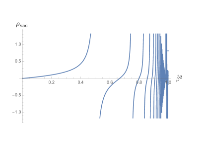
Figure 2: ${\rho_{\rm vac}}$ for the sine-Gordon model as a function of the coupling $\widehat{\beta}^{2}$.

$\bullet$   At the marginal point $\widehat{\beta}^{2}=1$, ${\rho_{\rm vac}}$ is indeterminate. In fact between the free fermion point and the marginal one, where the spectrum consists only of the Thirring fermion, ${\rho_{\rm vac}}$ undergoes an infinite number of oscillations around zero.

$\bullet$   The above ${\rho_{\rm vac}}$ is consistent with Property 3 in its supersymmetric version. Although the notion of a fermion verses boson is ambiguous in $2D$, supersymmetry is not ambiguous. For $\widehat{\beta}^{2}=2/3$ the sine-Gordon model has a hidden ${\cal N}=2$ supersymmetry BLfractional , and indeed ${\rho_{\rm vac}}=0$ at this coupling. However this explains only one of the points where ${\rho_{\rm vac}}=0$. The other such points also have an explanation. In BernardLeClair it was shown that the sine-Gordon theory has non-local conserved charges $Q_{\pm},\overline{Q}_{\pm}$ that satisfy the quantum affine algebra ${\cal U}_{q}(\widehat{{\rm su}(2)})$ where $q=e^{-i\pi/\widehat{\beta}^{2}}$. When

$$\widehat{\beta}^{2}=p/(p+1),$$ (84)

where $p\geq 1$ is an integer, $q=-e^{-i\pi/p}$ is a root of unity. In Vafa it was shown that when $p$ is an even positive integer, the quantum affine algebra corresponds to a fractional supersymmetry, where the conserved charges have spin $\pm 1/p$. For general $p$, “fractional supersymmetry” refers to the fact that mathematically the hamiltonian $H$ is in the center of the universal enveloping quantum affine algebra, namely $[Q,H]=0$ for all the non-local charges $Q$. For instance, for $p=4$, $Q^{4}=H$, where $Q^{4}=Q_{+}Q_{-}Q_{+}Q_{-}+....$ is quartic in the conserved charges $Q_{\pm}$. If $Q|{\rm vac}\rangle=0$, then ${\rho_{\rm vac}}$ should be zero, and indeed it is for these values of $\widehat{\beta}$.

$\bullet$   Finally let us turn to the divergences in (82). Namely ${\rho_{\rm vac}}$ diverges at the odd $p$ points in (84), and this is more difficult to explain. For $p=1$, above we attributed this divergence to the $\log m\beta$ term in the free fermion theory, however for higher $p$ this explanation does not apply since the theory is not free. In Mingling we proposed that these divergences arise from a kind of “resonance” phenomenon. Namely the terms in (15) with $c_{\mathfrak{p}>D}$ generally arise from conformal perturbation theory about the UV. It can happen that these perturbative terms can mix with the ${\rho_{\rm vac}}$ term $c_{{\scriptscriptstyle{D}}}r^{D}$ if the anomalous dimension of operators that perturb the UV CFT are rational, such that higher terms can give an additional power $\mathfrak{p}=D$ in (15). For the sine-Gordon model this this resonance condition is simply $p$ an odd integer in (84) Mingling . However a better understanding of this divergence is desirable, at least in order to understand whether it can happen in higher dimensions. We suspect this is unlikely since anomalous dimensions are not rational in general for $D>2$.

V.3 Affine Toda field theories

In this section we consider a model of multiple interacting scalar fields with exponential interactions, namely the affine Toda theories based on SU(N+1). The S-matrices were first proposed in Fateev . For a comprehensive treatment and review of such theories see Braden , and references therein. In 2D such a theory is super-renormalizable. We present it to illustrate the LMB mechanism in this case where each particle corresponds to a scalar field in the theory. It is also subject to a weak coupling expansion, which can be compared with the exact result. We will carry this out to lowest order in a semi-classical approximation. We will also provide some evidence for a phase transition at the self-dual point.

V.3.1 Exact ${\rho_{\rm vac}}$

Let $G$ denote a finite dimensional Lie algebra of ADE type, i.e. simply laced, of rank $\mathfrak{r}$. Denote the simple roots as $\bm{\alpha}_{i}$, $i=1,2,\dots\mathfrak{r}$:

$$\bm{\alpha}_{i}=(\alpha_{i}^{1},\alpha_{i}^{2},\ldots,\alpha_{i}^{r})\equiv\{\alpha_{i}^{a},~{}a=1,2,\ldots\mathfrak{r}\}$$ (85)

Introduce $\mathfrak{r}$ real scalar fields $\bm{\phi}$:

$$\bm{\phi}=(\phi^{1},\phi^{2},\ldots,\phi^{r})\equiv\{\phi^{a},~{}a=1,2,\ldots,\mathfrak{r}\}$$ (86)

such that $\bm{\alpha}_{i}\cdot\bm{\phi}=\sum_{a=1}^{\mathfrak{r}}\alpha_{i}^{a}\phi^{a}$. The untwisted affine Lie algebra $\widehat{G}$ has one additional root $\bm{\alpha}_{0}$: $\bm{\alpha}_{0}=-\sum_{i=1}^{\mathfrak{r}}\bm{\alpha}_{i}$. For simply laced $G$ one can take $\bm{\alpha}_{i}^{2}=2~{}~{}\forall i$. With these definitions one can define the $2d$ Euclidean action

$${\cal S}=\int d^{2}x\left(\dfrac{1}{8\pi}\partial\bm{\phi}\cdot\partial\bm{\phi}+V(\bm{\phi})\right),~{}~{}~{}~{}~{}V(\bm{\phi})=\mu\,\sum_{i=0}^{r}e^{b\,\bm{\alpha}_{i}\cdot\bm{\phi}}.$$ (87)

The $1/8\pi$ normalization corresponds to standard $2d$ conformal field theory conventions where $\langle\phi^{a}(x)\phi^{b}(0)\rangle=-\delta_{ab}\log x^{2}$ which fixes the convention for the coupling $b$. In particular in the QFT, $V(\bm{\phi})$ is a strongly relevant perturbation of anomalous scaling dimension $-2b^{2}$.

Henceforth for concreteness we specialize to $G=A_{N}={\rm SU}(N+1)$ where $\mathfrak{r}=N$. Then the Cartan matrix for ${\rm SU}(N+1)$ is $C_{ij}=\bm{\alpha}_{i}\cdot\bm{\alpha}_{j}$, where the non-zero values for $i\neq j$ are $C_{ij}=-1$ for $i=j\pm 1$ ($i,j\in\{1,2,\ldots,N\}$). From the classical mass matrix based on the quadratic term in the potential,

$$V(\bm{\phi})=\ldots+\tfrac{1}{2}\left[M^{2}\right]_{ab}\phi^{a}\phi^{b}+\ldots$$ (88)

one finds

$$\left[M^{2}\right]_{ab}=4\pi\mu\,b^{2}\left(\sum_{i=0}^{N}\alpha_{i}^{a}\alpha_{i}^{b}\right).$$ (89)

It is diagonal $M^{2}={\rm diag}(m_{1}^{2},m_{2}^{2},\ldots m_{N}^{2})$, with masses

$$m_{a}^{2}=16\pi\mu\,b^{2}\,\sin^{2}\left(\dfrac{a\pi}{N+1}\right).$$ (90)

Let $S_{11}(\theta)$ denote the S-matrix for the particle of mass $m_{1}$ with itself:

$$S_{11}=\prod_{\alpha}f_{\alpha}=f_{\tfrac{2}{h}}\,f_{-\tfrac{2\gamma}{h}}\,f_{\tfrac{2(\gamma-1)}{h}},~{}~{}~{}h=N+1,~{}~{}~{}~{}~{}~{}\gamma=\dfrac{b^{2}}{1+b^{2}}$$ (91)

$h$ is the dual Coxeter number, and $f_{\alpha}(\theta)$ is defined above. Then

$$\mathfrak{g}=2\sum_{\alpha}\sin\pi\alpha=-8\sin(\pi/h)\sin(\pi\gamma/h)\sin(\pi(1-\gamma)/h).$$ (92)

Based on equation (17), one then finds

$${\rho_{\rm vac}}=-\dfrac{m_{1}^{2}}{16\,\sin(\pi/h)\,\sin(\pi\gamma/h)\,\sin(\pi(1-\gamma)/h)}.$$ (93)

There are some interesting features here also. In the zero coupling limit this leads to

$$\lim_{b\to 0}\,{\rho_{\rm vac}}=-\dfrac{(N+1)\,m_{1}^{2}}{16\pi\,b^{2}\,\sin^{2}\left(\tfrac{\pi}{N+1}\right)}+{\cal O}(1).$$ (94)

An interesting feature is that if the physical mass $m_{1}$ is fixed then because of the $1/b^{2}$ dependence it appears non-perturbative. However this may simply be a result of expressing in terms of $m_{1}$ since $m_{1}\propto b^{2}$ in (90). Expanding ${\rho_{\rm vac}}$ for $N=1$ (the sinh-Gordon model) one finds

$$\lim_{b\to 0}\,{\rho_{\rm vac}}=-m_{1}^{2}\left(\dfrac{1}{8\pi b^{2}}-\dfrac{1}{8\pi}-\dfrac{\pi b^{2}}{48}+\dfrac{\pi b^{4}}{48}-\dfrac{(60+7\pi^{2})\pi b^{6}}{2880}+\ldots\right)~{}~{}~{}~{}~{}(N=1)$$ (95)

Again it would be interesting to understand this expansion in perturbation theory. As previously stated, the leading $1/b^{2}$ term may appear non-perturbative, however in terms of $\mu$ instead of $m_{1}\propto b^{2}$ it is not. Remarkably, this was already understood using the S-matrix bootstrap and Feynman diagrams by Destri-deVega DestriDeVega . They calculated all tadpole diagrams and showed that all the UV divergences could be absorbed into physical masses.

V.3.2 Semi-classical analysis

.

Let us show that weak coupling limit in (94) is in perfect agreement with a semi-classical analysis. The vacuum energy in this limit is simply the minimum of the potential:

$$\dfrac{\delta V}{\delta\bm{\phi}}\Bigl{|}_{\bm{\phi}=\bm{\phi}_{0}}=0$$ (96)

which implies $\bm{\phi}_{0}=0$. Thus

$$\lim_{b\to 0}\,{\rho_{\rm vac}}=V(\bm{\phi}_{0})=(N+1)\mu.$$ (97)

Expressing $\mu$ in terms of $m_{1}$ as given in (90) one obtains precisely (94), apart from the sign. We attribute this sign discrepancy to the fact that in the thermal TBA channel in 2D, the particles must be treated as fermions rather than bosons. The higher order terms in (95) must arise from the corrections to this semi-classical approximation.

V.3.3 Evidence for a phase transition at $b=1$.

It turns out ${\rho_{\rm vac}}$ is always negative. The case $N=1$ corresponds to the sinh-Gordon model. A plot of ${\rho_{\rm vac}}$ in this case is shown in Figure 3, and is very similar for other $N$. More importantly, it suggests a quantum phase transition in the vicinity of $b=1$, since increasing $b$ starting from zero ${\rho_{\rm vac}}$ increases until $b=1$ then it starts to decrease. This property relates to a long-term open question concerning the properties of the sinh-Gordon above the self-dual point of the S-matrix at $b=1$. The same issue arises for all the affine Toda theories. The S-matrices and ${\rho_{\rm vac}}$ satisfy the strong-weak coupling duality $b\to 1/b$, however the action has no such symmetry. Thus the definition of the sinh-Gordon theory by analytic continuation from the perturbative region $0<b<1$ to $1<b<\infty$ using the duality is questionable. This has been studied in great detail using various methods in Konik , and significant evidence for some phase transition at $b=1$ is seen, however a description of the theory for $b>1$ was beyond their scope, except that it was proposed there that the theory is massless. Recently a proposal for the sinh-Gordon beyond the self-dual point was proposed in BLfreezing by invoking a Coulomb background that is shifted from the Liouville one, and this reproduces some known results in disordered systems; however a complete description of the theory above $b=1$ is still lacking. Nevertheless it is interesting that ${\rho_{\rm vac}}$ gives some evidence for such a phase transition if our interpretation is correct.

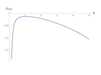
Figure 3: ${\rho_{\rm vac}}$ for the sinh-Gordon model (N=1) as a function of $b$ based on equation (93).

VI QCD in 4D:    Estimation of ${\rho_{\rm vac}}$ from numerical lattice results for 3 flavors.

Lattice QCD at finite temperature is well enough developed by now that its data can be used to provide a rough estimate of ${\rho_{\rm vac}}$ based on the proposal of this article. We refer to the articles Karsch ; Bazavov . Bazavov et. al. considered 3 flavors with masses $m_{u}=m_{d}=m_{s}/30$ where $m_{s}\approx 90\,{\rm MeV}$ is the strange quark mass, which is fit to the $s\overline{s}$ meson mass of $695\,{\rm MeV}$. Data on the pressure is presented in Figure 4. The critical de-confinement temperature is $T_{c}\approx 155\,{\rm MeV}$. In connection with the c-theorem, from this figure one sees that $(\rho-3p)>0$, thus $c(r)$ decreases with increasing $r$ based on (14).

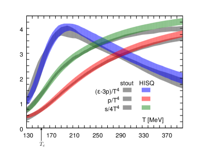
Figure 4: $p\beta^{4}$ as a function of temperature. (Taken from Bazavov ).

QCD is UV complete due to asymptotic freedom Wilczek ; Gross . We can thus predict $c_{\rm uv}$. Since each of the 8 gluons has 2 polarizations, and each quark has 3 colors, 2 spins, and has an anti-quark, for $n_{f}$ flavors

$$c_{\rm uv}=16+21\,n_{f}/2,~{}~{}~{}~{}~{}(c_{\rm uv}=47.5~{}~{}~{}~{}{\rm for}~{}~{}n_{f}=3).$$ (98)

The data in Figure 4 can be converted to $c(r)=-\beta^{4}{\cal F}/\chi(4)=p\beta^{4}/\chi(4)$ and is shown in Figure 5. There may be log corrections to the $c_{\rm vac}\sim r^{4}$ term as in (52), however for simplicity with ignore this. Fitting the data we obtain

$$c(r)\approx 42.72-1.468\cdot 10^{6}\,r^{2}+c_{4}\,r^{4},~{}~{}~{}~{}~{}c_{4}=1.409\cdot 10^{10}.$$ (99)

The fit approximately agrees with the prediction (98), and presumably is improved with additional higher temperature data. In particular, the above fit gives $c_{\rm uv}\approx 41.72$ compared to $47.5$ in (98). It’s also significant to point out that this fit is to data that is mostly at temperatures above $T_{c}$, and one can observe a change of behavior of $c(r)$ in the vicinity of $T_{c}$ where the ${\cal O}(r^{4})$ fit in equation (99) begins to fail.

In the Figure 5, $r=M\beta$ where $M=1\,{\rm MeV}$. Thus (17) gives

$${\rho_{\rm vac}}=-c_{4}\,\chi(4)\,M^{4}\approx-\left(200\,{\rm MeV}\right)^{4}\approx-\left(1.3\,T_{c}\right)^{4}\approx-\left(2.2\,m_{s}\right)^{4}.$$ (100)

Note that ${\rho_{\rm vac}}$ is negative and the scale is roughly set by the strange quark mass $m_{s}$. Perhaps it is negative since the strange quark is a fermion and at least for free theories ${\rho_{\rm vac}}$ is negative according to (52). It is interesting that $200\,{\rm MeV}$ is extracted from high temperature data above $T_{c}$ which a priori does not assume anything about the de-confinement phase transition at the lower temperature.

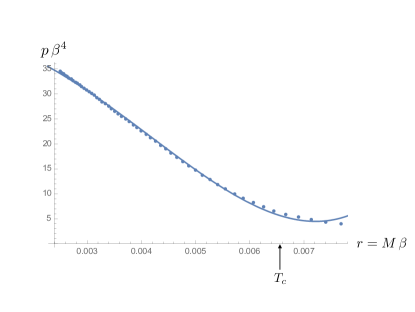
Figure 5: The pressure $p\,\beta^{4}$ as a function of $r=M\beta$ where $M=1\,{\rm MeV}$. Data points are from Bazavov which refer to Figure 4, and the continuous curve is the fit (99).

VII Conclusions

We have presented a non-perturbative definition of the vacuum energy density ${\rho_{\rm vac}}$ in any spacetime dimension based on Thermodynamics, i.e. in the Thermal channel for a cylinder. For massive free theories we established modularity in $D$ spacetime dimensions, namely the equivalence to calculations in a spatially compactified channel SpC . In 2D, for integrable QFT’s one can calculate ${\rho_{\rm vac}}$ exactly with the TBA, and we presented several illustrative examples. The Thermal channel enjoys certain advantages over the SpC channel since the integrals are not divergent from the beginning, and it is easier to identify both pressure $p$ and energy density $\rho$. We applied these ideas to QCD and extracted ${\rho_{\rm vac}}$ for 3 flavor QCD from high temperature lattice data and obtained a negative result ${\rho_{\rm vac}}\approx-(200\,{\rm MeV})^{4}$.

We close with suggestions for possible further developments.

$\bullet$   The TBA in 2D is based solely on the S-matrix and was efficient at calculating the exact ${\rho_{\rm vac}}$. It would thus be desirable to work with a formulation of quantum statistical mechanics based on the S-matrix, since all renormalizations of the theory can be carried out in the usual way at zero temperature and have an S-matrix that is already expressed, or measured, in terms of physical masses and couplings. There exists such a formulation in any dimension Dashen which leads to the simple formula for the partition function

$$Z=Z_{0}+\dfrac{1}{2\pi}\int_{0}^{\infty}dE\,\,e^{-\beta E}\,{\rm Tr}\,\Im\left(\partial_{E}\log\widehat{S}(E)\right).$$ (101)

where $\widehat{S}$ is the S-matrix quantum operator, and $Z_{0}$ is the free, unperturbed partition function. Unfortunately it turns out to be quite a deal of work to turn the above formula into something useful, although some results for non-relativistic theories were obtained in PyeTon ; PyeTon2 . It may be useful to explore this further for relativistic theories in order to perhaps understand if a version of the LMB is valid.

$\bullet$   This work was motivated by the Cosmological Constant Problem which we remarked on in Section II. We argued that depending on one’s assumptions of what the ultimate resolution will be, approaches to the problem can vary significantly. For this reason we formulated a well-defined version of the problem where the resolution would amount to properly computing ${\rho_{\rm vac}}$ in flat Minkowski space, which is actually close to its original version Weinberg . Although a big improvement over the naive 120 orders of magnitude error, for QCD the value we obtained is still too high to explain the measured value (5). Does this rule out our proposal for the CCP? We wish to argue this is not completely settled. First of all, the sign of ${\rho_{\rm vac}}$ for interacting theories is not easily predictable, it is negative for QCD, so there may be cancellations when one considers the complete Standard Model of particle physics. This is evident for instance for the massive Thirring model considered above where ${\rho_{\rm vac}}$ undergoes an infinite number of oscillations around zero as one approaches the marginal point (Figure 2). Secondly, perhaps there is exists a version of the LMB mechanism in higher dimensions, wherein all S-matrices can be bootstrapped from that of the lightest particle and the ${\rho_{\rm vac}}$ scale is set by the lightest particle as for integrable 2D theories. This appears challenging to study, however some promising results were cultured out of the Swampland Montero1 ; Montero2 based on very different ideas in connection with charged black holes. Thirdly, perhaps one needs to impose the constraint that ${\rho_{\rm vac}}$ for stable particles are all that contribute to the cosmological constant. If one could justify the LMB property to higher dimensions, this would point to neutrinos to explain the measured $\rho_{\Lambda}$ in (5), and indeed $0.003\,eV$ is close to proposed neutrino masses neutrino .

$\bullet$   In LeClairMussardo , $\langle T_{\mu\nu}\rangle_{\beta}$ at finite temperature was computed using form-factors in $2D$. It is worth exploring if such a form-factor approach can provide an efficient means to calculate ${\rho_{\rm vac}}$ in higher dimensions.

$\bullet$   We have shown that a restricted modular invariance, which is a trivial subgroup of the modular group $SL(2,\mathbb{Z})$ that interchanges the Thermal and SpC channels we referred to as Modularity, is valid on the cylinder in $D=2$ and $4$ spacetime dimensions for free massive theories. It would be very interesting to establish complete $SL(2,\mathbb{Z})$ invariance on the torus, which has two periodic directions, for non-conformal theories in arbitrary $D$ spacetime dimensions. Some recent results concerning this were obtained by Kostov in 2D Kostov . For CFT’s in higher dimensions see Shaghoulian .

VIII Acknowledgements

We wish to thank Denis Bernard, Ivan Kostov, Peter Lepage, Giuseppe Mussardo and Matthias Neubert for discussions.

References

- (1) S. Weinberg, The Cosmological Constant Problem, Rev. Mod. Phys. 61 (1989) 1.
- (2) J. Martin, Everything you always wanted to know about the Cosmological Constant Problem (But were afraid to ask). Comptes Rendus Physique, vol 13, (2012) 566, arXiv:1205.3365.
- (3) S. M. Carroll, The Cosmological Constant, Living reviews in relativity 4.1 (2001): 1-56.
- (4) See e.g. http://pdg.lbl.gov/2012/reviews/rpp2012-rev-astrophysical-constants.pdf
- (5) M. D. Schneider, What’s the Problem with the Cosmological Constant? Philosophy of Science 87 (2020): 1-20.
- (6) A. LeClair, Mingling of the infrared and ultraviolet and the “cosmological constant” for interacting QFT in 2d, JHEP 5( 2023), 1-18. arXiv:2301.09019 [hep-th].
- (7) Al. B. Zamolodchikov, Thermodynamic Bethe Ansatz in relativistic models: scaling 3-state Potts nd Lee-Yang models, Nucl. Phys. B342 (1990) 695.
- (8) C. N. Yang and C. P. Yang, Thermodynamics of a one-dimensional system of bosons with repulsive delta-function interaction, J. Math. Phys. 10 (1969) 1115.
- (9) T. Klassen and E. Melzer, The thermodynamics of purely elastic scattering theories and conformal perturbation theory, Nucl. Phys. B350 (1991) 635.
- (10) G. Mussardo, Statistical Field Theory, An Introduction to Exactly Solved Models in Statistical Physics, 2010, Oxford University Press.
- (11) A. B. Zamolodchikov, Irreversibility of the flux of the renormalization group in a 2D field theory, Pis’ma Eksp. Teor. Fiz. 43 (1986) 565.
- (12) A. LeClair and C. Vafa, Quantum affine symmetry as generalized supersymmetry, Nuclear Physics B401 (1993) 413, [arXiv:hep-th/9210009].
- (13) L. Giardello, M. T. Grisaru and P. Salomonson, Temperature and Supersymmetry,, Nuclear Physics B178 (1981): 331.
- (14) J. Cardy, Conformal Invariance and Statistical Mechanics, Les Houches 40 (1988).
- (15) G. Mussardo and P. Simon, Bosonic-type S-matrix, vacuum instability, and CDD ambiguity, Nucl.Phys. B578 (2000) 527, [arXiv:hep-th/9903072].
- (16) C. Destri and H. J. de Vega, New exact results in Affine Toda field theories: Free energy and wave- function renormalizations, Nuclear Physics B358 (1991) 251-294.
- (17) S. Coleman, Quantum sine-Gordon model as the massive Thirring model, Phys. Rev. D11 (1975) 2088.
- (18) A. B. Zamolodchikov and A. B. Zamolodchikov, Factorized S-matrices in two dimensions as the exact solutions of certain relativistic quantum field theory models, Annals of Physics 120 (1979) 273.
- (19) D. Bernard and A. LeClair The fractional supersymmetric sine-Gordon models, Phys. Lett. B247 (1990) 309.
- (20) D. Bernard and A. LeClair, Quantum group symmetries and non-local currents in 2D QFT, Communications in Mathematical Physics 142 (1991): 99-138.
- (21) A. E. Arinshtein, V. A. Fateev, and A. B. Zamolodchikov, Quantum S-matrix of the (1+1) dimensional Toda chain, Phys. Lett. 87B (1979) 389.
- (22) H. W. Braden, E. Corrigan, P. E. Dorey, and R. Sasaki, Affine Toda field theory and exact S-matrices, Nucl. Phys. B338 (1990) 689.
- (23) R. Konik, M. Lájer, and G. Mussardo, Approaching the self-dual point of the sinh-Gordon model, JHEP 2021.1 (2021): 1-85.
- (24) D. Bernard and A. LeClair, The sinh-Gordon model beyond the self dual point and the freezing transition in disordered systems, JHEP 2022 (2022) 22, arXiv:2112.05490 [hep-th].
- (25) F. Wilczek, QCD and asymptotic freedom: Perspectives and prospects, International Journal of Modern Physics A 8.08 (1993): 1359.
- (26) D. J. Gross, The discovery of asymptotic freedom and the emergence of QCD, International Journal of Modern Physics A 20.25 (2005): 5717.
- (27) F. Karsch, Lattice QCD at Finite Temperature and Density, Nucl. Phys. B (Proc. Suppl.) 83 (2000) 14, arXiv:hep-lat/9909006.
- (28) A. Bazavov, T. Bhattacharya, C. DeTar, H. T. Ding, S. Gottlieb, R. Gupta, ….. and HotQCD Collaboration. (2014). Equation of state in (2+ 1)-flavor QCD. Physical Review D90 (2014) 094503, arXiv:1407.6387 [hep-lat]
- (29) R. Dashen, S.-K. Ma and H. J. Bernstein, S-matrix formulation of statistical mechanics, Phys. Rev. 187 (1969) 345.
- (30) P.-T. How and A. LeClair, Critical point of the two-dimensional Bose gas: an S-matrix approach, Nucl. Phys. B824 (2010) 415, arXiv:0906.0333 [math-ph].
- (31) P.T. How and A. LeClair, S-matrix approach to quantum gases in the unitary limit II: the three-dimensional case, J. Stat. Mech. (2010) P07001, arXiv:1004.5390 [cond-mat.quant-gas].
- (32) M. C. Gonzalez-Garcia and Y. Nir, Neutrino masses and mixing: evidence and implications, Rev. Mod. Phys. 75 (2003) 345, arXiv:hep-ph/0202058 .
- (33) A. LeClair and G. Mussardo, Finite Temperature Correlation Functions in Integrable QFT, Nucl.Phys. B552 (1999) 624, arXiv:hep-th/9902075.
- (34) M. Montero, T. Van Riet and G. Venken, Festina Lente: EFT Constraints from Charged Black Hole Evaporation, JHEP 2020.1: 1-50, arXiv:1910.01648 [hep-th].
- (35) M. Montero, C. Vafa, T. Van Riet and G. Venken, The FL bound and its phenomenological implications, JHEP 10 (2021) 009, arXiv:2106.07650 [hep-th].
- (36) I. Kostov, Two-dimensional massive integrable models on a torus, JHEP 9 (2022) 119, arXiv:2205.03359 [hep-th].
- (37) E. Shaghoulian, Modular forms and a generalized Cardy formula in higher dimensions, Physical Review D 93.12 (2016) 126005, arXiv:1508.02728 [hep-th].