A lattice Boltzmann approach for acoustic manipulation

Abstract

We employ a lattice Boltzmann method to compute the acoustic radiation force produced by standing waves on a compressible object. Instead of simulating the fluid mechanics equations directly, the proposed method uses a lattice Boltzmann model that reproduces the wave equation, together with a kernel interpolation scheme, to compute the first order perturbations of the pressure and velocity fields on the object’s surface and, from them, the acoustic radiation force. The procedure reproduces with excellent accuracy the theoretical expressions by Gor’kov and Wei for the sphere and the disk, respectively, even with a modest number of lattice Boltzmann cells. The proposed method shows to be a promising tool for simulating phenomena where the acoustic radiation force plays a relevant role, like acoustic tweezers or the acoustic manipulation of microswimmers, with applications in medicine and engineering.

I Introduction

The manipulation of particles by acoustic oscillating fields in aqueous media has won relevance in recent years because of its applications in biotechnology, health, and marine research, among others Mohanty et al. (2020); Ahmed et al. (2021); Jinjie et al. (2009); Marzo et al. (2015). Just like optical tweezers Ashkin (1970); Gutsche et al. (2008), standing acoustic waves can push objects immersed in a fluid to the nodes (or anti-nodes) of the oscillating field Bruus (2006), with many practical advantages. Indeed, particles can be manipulated by using acoustic standing waves that only require $\simeq 10^{5}$ times less power than their optical counterpart Ozcelik et al. (2018). Indeed, acoustic tweezers can move objects from 100 nm to 10 mm in size by using acoustic wave intensities between $10^{-2}$ and 10 W/cm². Recently, acoustic transducers were used to extract kidney stones from a pig in non-invasive surgery, demonstrating the potential of acoustical tweezers in medicine Ghanem et al. (2020). In a recent experiment, Zhang et. al. showed how nodal planes of acoustic standing waves could be used as virtual walls to induce a rolling motion of self-assembled microswimmers Zhang et al. (2022). More applications for acoustic tweezers can be found in a recent review Andrade et al. (2018).

Historically, after the seminal work of Louis V. King King (1934, 1935), L.P. Gor’kov developed an improved model for the calculation of the time-averaged force by a plane acoustic wave on a spherical particle immersed in an ideal (inviscid, isentropic and irrotational) fluid Gor’kov (1962). Interestingly, when the wavelength is much larger than the particle size, the acoustic force can be cast into an effective potential, the so-called Gor’kov potential Gor’kov (1962). The two-dimensional case was studied by Junru Wu and Gonghuan Du in 1990 Wu and Du (1990) and later by Wei Wei et.al. in 2004 Wei et al. (2004), who used scattering theory to solve the wave equation for a compressible cylinder of infinite height in a standing wave (For an extensive theoretical review, see Bruus (2006) and Bruus (2011, 2012a, 2012b)).

All these theoretical studies rely on the assumption that the relevant macroscopic fields, like pressure and velocity, can be written as a perturbative expansion, where the first order contributions $p_{1}$ for the pressure and $\vec{u}_{1}$ for the velocity satisfy the wave equation. Although the acoustic radiation force depends on second order contributions, they can be written in terms of $p_{1}$ and $\vec{u}_{1}$, opening the possibility of solving the wave equation - instead of the Navier-Stokes equations (NSE) - for $p_{1}$ and $\vec{u}_{1}$, and use those results to compute the acoustic radiation force. Because the wave equation can be easily solved with large precision, such a procedure will require less computational effort than a direct NSE simulation (where $p_{1}$ and $\vec{u}_{1}$ are just first order perturbations of the computed pressure and velocity fields), allowing to simulate complex shapes in 2D and 3D as required for today’s microfluidics applications.

Here, we show how to use a lattice Boltzmann method (LBM) that simulates the wave equation Chopard et al. (1997) to compute the acoustic radiation force on an object immersed in an inviscid fluid. Our approach reproduces with great accuracy the theoretical predictions by Gor’kov Gor’kov (1962) and Wei Wei et al. (2004) at much lower computational costs than previous LBM approaches simulating the full Navier-Stokes equations Cosgrove et al. (2004). The remainder of this paper is organized as follows: in Sec. II, the acoustic radiation force is derived following Gor’kov Gor’kov (1962). Next, Sec. III reviews the theoretical deduction of Gor’kov’s potential, together with an analogous development by us for the 2D case in Sec. ‘IV. Next, Chopard’s LBM model for waves is briefly explained in Sec. V with some benchmarks to validate our implementation in our simulation code. Our results for the acoustic radiation force on a sphere and a disk are reported in Sec. VII, showing that the computed forces follow the theoretical predictions with excellent accuracy.

II The second order acoustic radiation force

Consider an inviscid and compressible fluid in an irrotational flow with pressure $P$, density $\rho$ velocity $\vec{u}$ and momentum $\vec{J}=\rho\vec{u}$. The fluid is described by the mass conservation law

$$\frac{\partial\rho}{\partial t}+\vec{\nabla}\cdot\vec{J}=0\quad,$$ (1)

and Euler’s equation, which can be rewritten as a momentum conservation law,

$$\frac{\partial\vec{J}}{\partial t}=-\vec{\nabla}P+\vec{\nabla}\cdot\left(\vec{u}\otimes\vec{J}\right)=-\nabla\cdot\Pi\quad,$$ (2)

Here, $\Pi$ is the momentum flux density tensor, described as

$$\Pi=\mathbb{I}P+\vec{u}\otimes\vec{J}\quad.$$ (3)

By second Newton’s law, the force $\vec{F}$ acting on a static object immersed in the fluid equals the momentum exchange of the fluid across a volume control around the object (Manneberg, 2009, app. A)

$$\vec{F}=\int\frac{\partial\vec{J}}{\partial t}dV=-\oint\Pi\cdot\vec{dS}$$ (4)

Acoustic waves propagate in the fluid as small variations in pressure, density and velocity around steady values. So, the three fields can be written as follows:

$$\rho=\rho_{0}+\rho_{1}\quad,\quad P=p_{0}+p_{1}\quad,\quad\vec{u}=\vec{0}+\vec{u}_{1}\quad,$$ (5)

where $p_{1}$, $\rho_{1}$ and $\vec{u}_{1}$ are first order perturbations mentioned in Sec. I and we assume that $u_{0}=0$ (that is, the fluid is at rest). Since acoustic waves in a fluid are adiabatic compressions Elmore and Heald (1969), the first order pressure and density fluctuations are related as (Kinsler et al., 2000, p. 120)

$$p_{1}=c_{0}^{2}\rho_{1}\quad,$$ (6)

where $c_{0}^{2}$ is the adiabatic speed of sound of the fluid. By taking into account only first order contributions (as in Eq. (5)) Eqs. (2) and (1) are linearized as

$$\rho_{0}\frac{\partial\vec{u}_{1}}{\partial t}+\nabla p_{1}=0\quad,$$ (7a)

$$\frac{\partial\rho_{1}}{\partial t}+\rho_{0}\nabla\cdot\vec{u}_{1}=0\quad.$$ (7b)

By combining Eqs. (7), and (6), one obtains that $p_{1}$ fulfills a wave equation,

$$\frac{1}{c_{0}^{2}}\frac{\partial^{2}p_{1}}{\partial t^{2}}=\nabla^{2}p_{1}\quad.$$ (8)

Since the flow is irrotational, the velocity $\vec{u}=\vec{u}_{1}$ can be written as the gradient of a scalar velocity potential $\phi$, and Eq. (7a) transforms to give

$$\vec{u}_{1}=\nabla\phi\quad\mbox{,}\quad p_{1}=-\rho_{0}\frac{\partial\phi}{\partial t}\quad.$$ (9)

By replacing Eq. (9) into Eq. (7b), and using Eq. (6), we obtain that the velocity potential also fulfills a wave equation,

$$\frac{1}{c_{0}^{2}}\frac{\partial^{2}\phi}{\partial t^{2}}=\nabla^{2}\phi\quad.$$ (10)

In most experiments, the time scale of the object’s motion is much larger than the oscillation period, and thus, only the time average of the acoustic radiation force $\langle\vec{F}\rangle$ is relevant to the particle’s dynamics. If only first order fluctuations were considered (5), acoustic radiation force (4) would reduce to

$$\vec{F}=-\oint P\vec{dS}\quad,$$ (11)

because the term $\vec{u}\otimes\vec{J}$ is second order. Since the pressure perturbation oscillates harmonically in time, $p_{1}\propto e^{i\omega t}$, the time average of (11) automatically vanishes, and there is no first order contribution to the time-averaged force. The origin of that force lies, therefore, in higher-order contributions. Extending the fluctuations up to the second order,

$$\rho=\rho_{0}+\rho_{1}+\rho_{2}\quad,$$ (12a)

$$P=p_{0}+p_{1}+p_{2}\quad\text{ and}$$ (12b)

$$\vec{u}=\vec{0}+\vec{u}_{1}+\vec{u}_{2}\quad,$$ (12c)

one obtains that the gradient for the perturbations in the pressure field can be written only in terms of first order contributions (please see App. A for details) as

$$\nabla(P-p_{0})=\nabla\left(\frac{p_{1}^{2}}{2\rho_{0}c_{0}^{2}}-\frac{\rho_{0}}{2}u_{1}^{2}-\rho_{0}\frac{\partial\phi}{\partial t}\right)$$ (13)

leading to the following expression for the acoustic radiation force written in index notation:

$$\langle F_{i}\rangle=-\oint\left\langle\left(-\rho_{0}\frac{u_{1}^{2}}{2}+\frac{p_{1}^{2}}{2\rho_{0}c_{0}^{2}}\right)\delta_{ij}+\rho_{0}u_{1i}u_{1j}\right\rangle dS_{j}\quad,$$ (14)

where the triangular brackets $\left<\cdot\right>$ denote the time average. The contribution of the term $\rho_{0}\frac{\partial\phi}{\partial t}$ in Eq. (13) vanishes because the velocity potential $\phi\propto e^{i\omega t}$ is also harmonic. Eq. (14) computes the acoustic radiation force as a surface integral of quantities in terms of the first order contributions $p_{1}$ and $\vec{u}_{1}$, i.e. of those that fulfill wave equations (Eqs. (8) and (7a)). Eq. (14) allows us to compute the time-averaged acoustic radiation force on an immersed object from the pressure and velocity fields obtained by simulating the acoustic waves directly (Eqs. (8) and (7a)), instead of solving the full Navier-Stokes equations.

III Acoustic radiation force on a sphere

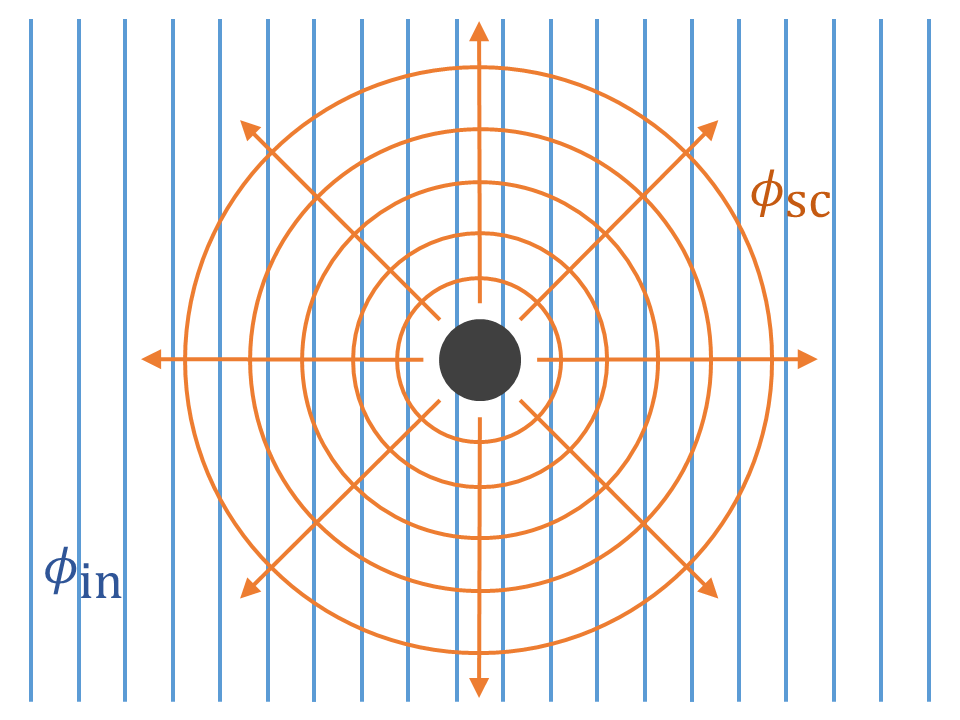
Figure 1: Decomposition into incident and scattering fields.

We aim to compute the average force by acoustic waves acting on a spherical object immersed in a liquid. Let us assume that the object’s radius $R_{p}$ is much smaller than the wavelength $\lambda$, i.e. $R_{p}\ll\lambda$. With this approximation, it is possible to solve Eq. (10) by dividing the potential, pressure and velocity fields into an incident and a scattered part as shown in Fig. 1 Gor’kov (1962), that is

$$\phi=\phi_{\text{in}}+\phi_{\text{sc}}\quad,\quad p_{1}=p_{\text{in}}+p_{\text{sc}}\quad,\quad\vec{u}_{1}=\vec{u}_{\text{in}}+\vec{u}_{\text{sc}}\quad.$$ (15)

The incident fields $(in)$ are the solution for the ongoing waves as if there was no spherical particle, while the scattered fields $(sc)$ are the differences between the total fields and the incident ones. By replacing (15) into (14), three main terms appear: The first one only depends on the incident fields and it does not contribute to the force; the second one depends on the scattered field $\phi_{\text{sc}}$ only, which will be proportional to $R_{p}^{6}$ and, thus, vanishes because of $R_{p}\ll\lambda$. The last and only surviving term depends on both $\phi_{\text{in}}$ and $\phi_{\text{sc}}$, and the force reduces to (see App. B for details)

$$\langle\vec{F}\rangle=-\rho_{0}\int\left\langle\vec{u}_{\text{in}}\left(\nabla^{2}\phi_{\text{sc}}-\frac{1}{c_{0}^{2}}\frac{\partial^{2}\phi_{\text{sc}}}{\partial t^{2}}\right)\right\rangle dV\quad.$$ (16)

The term between parenthesis is not zero because the object acts as a local source for the scattered field. Thus, a retarded-time multipolar expansion is proposed as a solution for $\phi_{\text{sc}}$,

$$\phi_{sc} =-\frac{a(t^{\prime})}{r^{\prime}}-\frac{\vec{A}(t^{\prime})\cdot\vec{r}^{\prime}}{r^{\prime 3}}+\dots$$

$$\approx\phi_{\text{mp}}+\phi_{\text{dip}}$$ (17)

where $\vec{r}^{\prime}=\vec{r}-\vec{v}t$ is the position of the center of the sphere, moving with velocity $\vec{v}$, and $t^{\prime}=t-r/c$ is a retarded time (with $t^{\prime}\approx t$ close to the object).

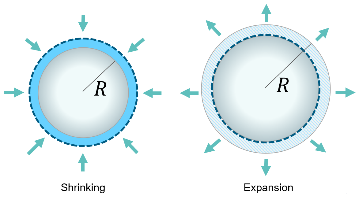
Figure 2: The object’s pulsating expansions and contractions induce spherical waves coinciding with the monopole term of the scattered velocity potential field.

The monopole term $\phi_{mp}=a(t)/r`$ can be found by assuming that the particle is able to compress and expand isotropically as shown in figure 2, changing its volume $V_{p}$ in response to the incident perturbations $p_{\text{in}}$ as

$$dp_{in}=-B_{p}\frac{dV_{p}}{V_{p}}\quad\mbox{, or}\quad\frac{\partial p_{in}}{\partial t}=-\frac{B_{p}}{V_{p}}\frac{dV_{p}}{dt}\quad,$$ (18)

with $B_{p}=c_{p}^{2}\rho_{p}$ the particle’s bulk modulus, $c_{p}$ the particle’s speed of sound and $\rho_{p}$ the particle’s density. Thus, by using (6),

$$\frac{dV_{p}}{dt}=-V_{p}\frac{c_{0}^{2}}{\rho_{p}c_{p}^{2}}\frac{\partial\rho_{\text{in}}}{\partial t}\quad.$$ (19)

Now, let us consider a spherical region $\Omega$ of radius $R_{\Omega}$ concentric to the sphere of radius $R_{p}$, with $\lambda\gg R_{\Omega}>R_{p}$. When the sphere expands, the mass flux leaving $\Omega$ through its surface $\partial\Omega$ equals the rate at which the sphere pushes fluid out of it,

$$\dot{m} =\frac{\partial}{\partial t}[(\rho_{0}+\rho_{\text{in}})V_{p}]$$ (20)

$$=\int_{\Omega}\dot{\rho}dV=\oint_{\partial\Omega}(\rho_{0}\gradient\phi_{\text{mp}})\cdot\hat{r}dS=4\pi a(t)\rho_{0}\quad,$$ (21)

with $\hat{r}$ the radial unitary vector. By (18) and (19) the total derivative in (20) becomes

$$\dot{m}=-V_{p}\frac{c_{0}^{2}}{\rho_{p}c_{p}^{2}}\frac{\partial}{\partial t}\left(\rho_{0}\rho_{\text{in}}+\frac{1}{2}\rho_{\text{in}}^{2}\right)+V_{p}\frac{\partial\rho_{\text{in}}}{\partial t}\mbox{ .}$$ (22)

Because the incident density is a perturbation of the total density of the fluid (i.e. $\rho_{0}\gg\rho_{\text{in}}$) the term $\frac{1}{2}\rho_{\text{in}}^{2}$ is much smaller than $\rho_{0}\rho_{in}$ and can be vanished. Therefore,

$$\dot{m}=4\pi a(t)\rho_{0}=V_{p}\frac{\partial\rho_{\text{in}}}{\partial t}\left(1-\frac{\rho_{0}c_{0}^{2}}{\rho_{p}c_{p}^{2}}\right)\quad,$$ (23)

and $a(t)$ turns out to be

$$a(t)=\frac{R_{p}^{3}}{3\rho_{0}}f_{1}\frac{\partial\rho_{\text{in}}}{\partial t}\quad\mbox{, with}\quad f_{1}=1-\frac{\rho_{0}c_{0}^{2}}{\rho_{p}c_{p}^{2}}\quad.$$ (24)

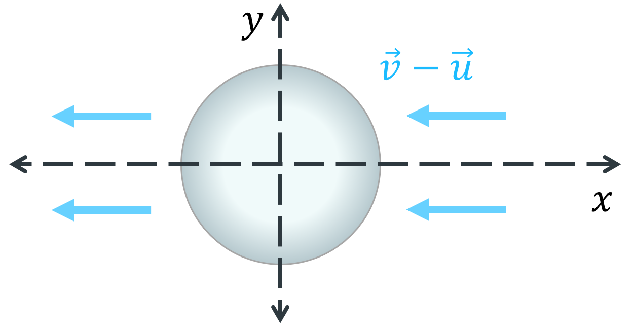
Figure 3: The accelerated motion of the object pushes the surrounding fluid and induces an added mass, i.e. a drag force proportional to the acceleration. That force allows to compute the dipole term of the scattered velocity potential field.

The dipole term

$$\phi_{\text{dip}}=-\vec{A}\cdot\vec{r}^{\prime}/r^{\prime 3}$$ (25)

comes into play when the sphere moves with a changing velocity $\vec{v}$ in a fluid with velocity $\vec{u}_{1}$. The velocity potential for this situation is the sum of the one for a sphere at rest in a fluid approaching with velocity $\vec{u}_{1}$ plus the one of a sphere moving with velocity $\vec{v}$ in a fluid at rest Pijush K. Kundu (1990),

$$\phi=\left(1+\frac{R_{p}^{3}}{2r`^{3}}\right)\left(\vec{u}_{1}\cdot\vec{r}^{\prime}\right)-\frac{R_{p}^{3}}{2r`^{3}}\left(\vec{v}\cdot\vec{r}^{\prime}\right)\quad.$$ (26)

The potential can be rearranged as

$$\phi=-\frac{R_{p}^{3}}{2r`^{3}}\left(\vec{v}-\vec{u}_{1}\right)\cdot\vec{r}^{\prime}+\left(\vec{u}_{1}\cdot\vec{r}^{\prime}\right)\quad,$$ (27)

where the last term is easily identified as the incident potential $\phi_{in}$, and the first term, as the one of a sphere moving in a fluid at rest with velocity $\left(\vec{v}-\vec{u}_{1}\right)$ (see Fig. 3). Indeed, by comparing $\phi_{in}$ in (27) with (25), one can identify

$$\vec{A}(r^{\prime})=-\frac{R_{p}^{3}}{2}\left(\vec{v}-\vec{u}_{1}\right)\quad.$$ (28)

On the one side and according to Pijush K. Kundu (1990), the force on the sphere produced by that potential is

$$F_{sc}=-M_{a}\left(\frac{\partial\vec{v}}{\partial t}-\frac{\partial\vec{u}_{1}}{\partial t}\right)\quad,$$ (29)

with

$$M_{a}=\frac{2}{3}\pi R_{p}^{3}\rho_{0}$$ (30)

the added mass for the sphere. On the other hand, if the sphere was made of fluid, it would move with velocity $\vec{v}=\vec{u}_{1}$ and, therefore, the force on the sphere from a potential $\phi=\vec{u}_{1}\cdot\vec{r}^{\prime}$ must be exactly the one we need to move that fluid sphere with an acceleration $\frac{\partial\vec{u}_{1}}{\partial t}$

$$F_{in}=M_{f}\frac{\partial\vec{u}_{1}}{\partial t}\quad\mbox{, with}\quad M_{f}=\frac{4}{3}\pi R_{p}^{3}\rho_{0}\quad.$$ (31)

The total force acting on the sphere of density $\rho_{p}$ and mass $M_{p}=4\pi R_{p}^{3}/3\rho_{p}$ is the sum of those two forces. Thus,

$$M_{p}\frac{\partial\vec{v}}{\partial t}=-M_{a}\left(\frac{\partial\vec{v}}{\partial t}-\frac{\partial\vec{u}_{1}}{\partial t}\right)+M_{f}\frac{\partial\vec{u}_{1}}{\partial t}\quad.$$ (32)

By replacing the expressions for the masses, we obtain

$$\left(\rho_{p}+\frac{\rho_{0}}{2}\right)\frac{\partial\vec{v}}{\partial t}=\frac{3}{2}\rho_{0}\frac{\partial\vec{u}_{1}}{\partial t}\quad.$$ (33)

If we assume that $\vec{v}=0$ when $\vec{u}_{1}=0$, integrating with respect to time $t$ gives us

$$\vec{v}=\frac{3\rho_{0}}{2\rho_{p}+\rho_{0}}\vec{u}_{1}\quad.\quad$$ (34)

and the vector field $\vec{A}(t)$ becomes

$$A(t)=\frac{R_{p}^{3}}{2}f_{2}\vec{u}_{1}\quad\mbox{, with}\quad f_{2}=\frac{2(\rho_{p}-\rho_{0})}{2\rho_{p}+\rho_{0}}\quad.$$ (35)

By plugging (24) and (35) into (III) and (16), and by solving the integration (see Appendix C for details), we have

$$\langle F_{i}\rangle=-\partial_{i}V_{p}\left(f_{1}\frac{1}{2\rho_{0}c_{0}^{2}}\langle p^{\prime 2}_{\text{in}}\rangle+\frac{3}{4}\rho_{0}f_{2}\langle v^{2}_{\text{in}}\rangle\right)=-\nabla U$$ (36)

where the potential $U$ is defined as

$$U=V_{p}\left(f_{1}\frac{1}{2\rho_{0}c_{0}^{2}}\langle p^{\prime 2}_{\text{in}}\rangle+\frac{3}{4}\rho_{0}f_{2}\langle v^{2}_{\text{in}}\rangle\right)\quad.$$ (37)

That is the Gor’kov potential. This potential is commonly used for acoustic levitation of small objects, even regardless of the object‘s shape as soon as $R_{0}\ll\lambda$ is satisfied. In the particular case of incident stationary waves,

$$p_{1}(x,t)=P_{a}\sin(\omega t)(\cos kx)\quad,$$ (38)

with $P_{a}$ the pressure amplitude, Eq. (9) give us the velocity as

$$u_{1x}(x,t)=-\frac{P_{a}}{c_{0}\rho_{0}}\cos\omega t\sin kx\quad.$$ (39)

By plugging (38) and (9) into the Gor’kov potential and solving the time-average integration, this potential for standing waves becomes

$$U=\frac{V_{p}P_{a}^{2}}{4\rho_{0}c_{0}^{2}}\left(f_{1}\cos^{2}kx+\frac{3}{2}f_{2}\sin^{2}kx\right)\quad.$$ (40)

The force can be gathered using (36), (24) and (35), leading to

$$F_{x}=-\frac{\pi R_{p}^{3}P_{a}^{2}k}{3\rho_{0}c_{0}^{2}}\Phi(\tilde{\rho},\tilde{\kappa})\sin 2kx\quad,$$ (41)

where $\tilde{\rho}=\rho_{p}/\rho_{0}$ , $\tilde{\kappa}=\kappa_{p}/\kappa_{0}$ and $\Phi(\tilde{\rho},\tilde{\kappa})$ is defined as

$$\Phi(\tilde{\rho},\tilde{\kappa})=\frac{5\tilde{\rho}-2}{2\tilde{\rho}+1}-\tilde{\kappa}\quad.$$ (42)

This is the theoretical result to compare with in 3D.

IV Acoustic radiation force on a disk

Instead of following the deduction by Wei Wei et al. (2004), let us follow the same procedure as in the previous section, but in two dimensions. As in (16), the acoustic radiation force can be computed from the scattered potential as

$$\langle F_{i}\rangle=-\rho_{0}\int\left\langle u_{\text{in}}^{i}\left(\nabla^{2}\phi_{sc}-\frac{1}{c_{0}^{2}}\frac{\partial^{2}\phi_{sc}}{\partial t^{2}}\right)\right\rangle dA\quad.$$ (43)

For a small disk, a retarded time multipolar expansion is also a good approximation in 2D,

$$\phi_{sc}=-a(t^{\prime})\log{r}-\frac{\vec{A}(t^{\prime})\cdot\vec{r}^{\prime}}{r^{\prime 2}}+\dots$$ (44)

with $\vec{r}^{\prime}=\vec{r}-\vec{v}t$ and $t^{\prime}=t-r/c\approx t$.

As in the 3D case, the scalar field $a(t)$ in the monopole term $\phi_{mp}=-a(t^{\prime})\log{r}$ can be found by assuming an isotropic compression and expansion of the disk due to the incident field $p_{\text{in}}$ by

$$dp_{in}=-B_{p}^{\text{2D}}\frac{dA_{p}}{A_{p}}\quad\mbox{, or}\quad\frac{\partial p_{in}}{\partial t}=-\frac{B_{p}^{\text{2D}}}{A_{p}}\frac{dA_{p}}{dt}\quad,$$ (45)

with $A_{p}$ the disk’s area, $B_{p}^{\text{2D}}=-AdP/dA=c_{p}^{2}\rho_{p}$ the particle’s bulk modulus in 2D. Furthermore, since $p_{in}=\rho_{in}c_{0}^{2}$, with $c_{0}$ the speed of sound in the fluid,

$$\frac{dA_{p}}{dt}=-A_{p}\frac{c_{0}^{2}}{\rho_{p}c_{p}^{2}}\frac{\partial\rho_{\text{in}}}{\partial t}\quad.$$ (46)

Consider a circular region $\Sigma$ of radius $R_{\Sigma}$ concentric to the disk with $\lambda\gg R_{\Sigma}>R_{p}$. On the one side, the mass flux leaving $\Sigma$ through its boundary $\partial\Sigma$ equals the rate at which the disk pushes fluid out of it

$$\dot{m}=\oint_{\partial\Sigma}(\rho_{0}\vec{\nabla}\phi_{mp})\cdot\hat{r}dl=2\pi a(t)\rho_{0}\quad,$$ (47)

On the other hand,

$$\dot{m}=\frac{\partial}{\partial t}[(\rho_{0}+\rho_{\text{in}})A_{p}]\approx A_{p}\frac{\partial\rho_{\text{in}}}{\partial t}\left(1-\frac{\rho_{0}c_{0}^{2}}{\rho_{p}c_{p}^{2}}\right)\mbox{ ,}$$ (48)

where we used (45) and (46). By equaling (47) and (48) by taking into account once again that $\frac{1}{2}\rho_{\text{in}}^{2}$ is much smaller than $\rho_{0}\rho_{\text{in}}$, we finally get

$$a(t)=\frac{R_{p}^{2}}{2\rho_{0}}\frac{\partial\rho_{in}}{\partial t}f_{1}\quad\mbox{, with}\quad f_{1}=1-\frac{\kappa_{p}}{\kappa_{0}}\quad.$$ (49)

Like in the 3D case the velocity potential around a disk traveling with velocity $\vec{v}$ in a fluid moving with velocity $\vec{u}_{1}$ is Pijush K. Kundu (1990)

$$\phi=\left(1+\frac{R_{p}^{2}}{r`^{2}}\right)\left(\vec{u}_{1}\cdot\vec{r}^{\prime}\right)-\frac{R_{p}^{2}}{r`^{2}}\left(\vec{v}\cdot\vec{r}^{\prime}\right)\quad,$$ (50)

that can be rearranged as

$$\phi=-\frac{R_{p}^{2}}{r`^{2}}\left(\vec{v}-\vec{u}_{1}\right)\cdot\vec{r}^{\prime}+\left(\vec{u}_{1}\cdot\vec{r}^{\prime}\right)\quad.$$ (51)

Here, again, the last term is the incident potential $\phi_{in}$, and the first term, the one of a disk moving in a fluid at rest with velocity $\left(\vec{v}-\vec{u}_{1}\right)$. By comparing $\phi_{in}$ in (51) with the dipole potential $\phi_{dip}=-\frac{\vec{A}(t)\cdot\vec{r}^{\prime}}{r^{\prime 2}}$ we identify

$$\vec{A}(r^{\prime})=-R_{p}^{2}\left(\vec{v}-\vec{u}_{1}\right)\quad.$$ (52)

The force on the disk produced by that potential is

$$F_{sc}=-M_{a}\left(\frac{\partial\vec{v}}{\partial t}-\frac{\partial\vec{u}_{1}}{\partial t}\right)\quad\mbox{, with}\quad M_{a}=\pi R_{p}^{2}\rho_{0}$$ (53)

the added mass for the disk Bernard (2015).

As in the 3D case, if the disk were made of fluid, it would move with velocity $\vec{v}=\vec{u}_{1}$ and, therefore, the force on the disk from a potential $\phi=\vec{u}_{1}\cdot\vec{r}^{\prime}$ must be exactly the one we need to move that fluid disk with an acceleration $\frac{\partial\vec{u}_{1}}{\partial t}$

$$F_{in}=M_{f}\frac{\partial\vec{u}_{1}}{\partial t}\quad\mbox{, with}\quad M_{f}=\pi R_{p}^{2}\rho_{0}\quad.$$ (54)

The total force acting on the disk of surface density $\rho_{p}$ and mass $M_{p}=\pi R_{p}^{2}\rho_{p}$ is the sum of those two forces. Thus,

$$M_{p}\frac{\partial\vec{v}}{\partial t}=-M_{a}\left(\frac{\partial\vec{v}}{\partial t}-\frac{\partial\vec{u}_{1}}{\partial t}\right)+M_{f}\frac{\partial\vec{u}_{1}}{\partial t}\quad.$$ (55)

By replacing the expressions for the masses, we obtain

$$\left(\rho_{p}+\rho_{0}\right)\frac{\partial\vec{v}}{\partial t}=2\rho_{0}\frac{\partial\vec{u}_{1}}{\partial t}\quad.$$ (56)

If we assume that $\vec{v}=0$ when $\vec{u}_{1}=0$, integrating with respect to time $t$ gives us

$$\vec{v}=\frac{2\rho_{0}}{\rho_{0}+\rho_{p}}\vec{u}_{1}\quad.\quad$$ (57)

and the vector field $\vec{A}(t)$ becomes

$$A(t)=R_{p}^{2}f_{2}\vec{u}_{\text{in}}\quad\mbox{, with}\quad f_{2}=\frac{\rho_{0}-\rho_{p}}{\rho_{0}+\rho_{p}}\quad.$$ (58)

After plugging in (49) and (58) into (43) and using the same standing incident wave written in (38) and (39), the two-dimensional Gor’kov’s potential takes the form

$$U=\frac{A_{p}p_{0}^{2}}{4\rho_{0}c_{0}^{2}}\left(f_{1}\cos^{2}kx+f_{2}\sin^{2}kx\right)$$ (59)

and the acoustic radiation force is

$$F_{x}=-\frac{\pi R_{p}^{2}P_{a}^{2}k}{4\rho_{0}c_{0}^{2}}\Phi(\tilde{\rho},\tilde{\kappa})\sin 2kx\quad,$$ (60)

where $\tilde{\rho}=\rho_{p}/\rho_{0}$, $\tilde{\kappa}=\kappa_{p}/\kappa_{0}$ and $\Phi(\tilde{\rho},\tilde{\kappa})$ is defined as

$$\Phi(\tilde{\rho},\tilde{\kappa})=\frac{3-\tilde{\rho}}{1+\tilde{\rho}}-\tilde{\kappa}\quad.$$ (61)

This last expression of the force (60) coincides with the equations 18 and 22 of the paper of Wei et al. (Wei et al., 2004, page. 204),validating this shorter deduction.

V Lattice-Boltzmann for acoustics

(a)

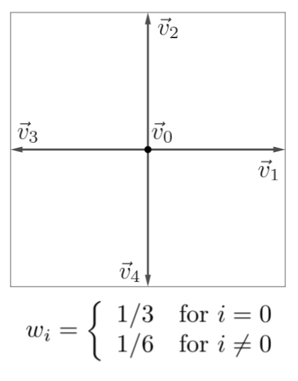
(b)

Figure 4: D3Q7 (a) and D2Q5 (b) velocity sets and their corresponding weights.

In an LBM, space is divided into cells, and a set of velocity vectors $\vec{v}_{i}$ allows for transport from each cell to the neighboring ones (Fig. 4).At each cell position $\vec{x}$ and associated with each velocity vector $\vec{v}_{i}$, there is at least one variable $f_{i}(\vec{x},t)$, called a distribution function, which represents the density of some hypothetical particles there, moving with that velocity and transporting information from cell to cell. At each time step, the $f_{i}$ are, first, mixed inside every cell into new values $f_{i}^{\rm new}$ by using Boltzmann’s transport equation (collision) and, then, transported to the neighboring cells along the vector they are associated with (advection). Because all the information for the collision is inside the cell itself and the advection is blind, all cells can evolve each time step in a fully independent way. That makes the LBM suitable to run in parallel on multiple CPUs or graphic cards Krüger and et. al (2017); Harting et al. (2004).

In an LBM for acoustics Chopard et al. (1997), the fluid density $\rho_{1}$, the momentum $\vec{J}_{1}=\rho_{0}\vec{u}_{1}$ and the pressure $p_{1}$ at any cell are computed as

$$\rho_{1}=\sum_{i}f_{i}\quad,\quad\vec{J}_{1}=\sum_{i}\vec{v}_{i}f_{i}\quad,\quad p_{1}=c^{2}\rho_{1}\quad,$$ (62)

where $c$ is the speed of sound for the fluid. At each time step $\Delta t$ every cell computes new values $f_{i}^{\rm new}$ for the distribution functions by using Boltzmann’s transport equation in the BGK (Bhatnagar-Gross-Krook) approximation,

$$f_{i}^{\rm new}(\vec{x},t)=\left(1-\frac{\Delta t}{\tau}\right)f_{i}+\left(\frac{\Delta t}{\tau}\right)f_{i}^{eq}\quad\mbox{, with}\quad\tau=\frac{1}{2}\mbox{,}$$ (63)

where the equilibrium values $f_{i}^{eq}$ are computed from the macroscopic fields (62). In contrast with LBM schemes for fluids, $\tau=1/2$ is perfectly stable for acoustics and other linear equations Mendoza and Muñoz (2008); Velasco et al. (2019). Next, the new values $f_{i}^{\rm new}$ are transported to the neighboring cells as

$$f_{i}(\vec{x}+\Delta t\vec{v}_{i})=f_{i}^{\rm new}(\vec{x},t)\quad.$$ (64)

By performing a Chapman-Enskog expansion it is shown that the macroscopic fields (62) satisfy in the continuous limit the following conservative equations Mendoza and Muñoz (2008):

$$\partialderivative{\rho_{1}}{t}+\divergence{J_{1}}=0\quad,$$ (65a)

$$\partialderivative{\vec{J}_{1}}{t}+\divergence{\Pi^{(0)}}=0\quad,$$ (65b)

with

$$\Pi^{(0)}=\sum_{i}\vec{v}_{i}\otimes\vec{v}_{i}f_{i}^{eq}\quad.$$ (66)

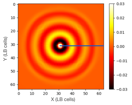
Figure 5: Lattice Boltzmann simulation of the 3D spherical waves produced by a point source after 60 time steps.

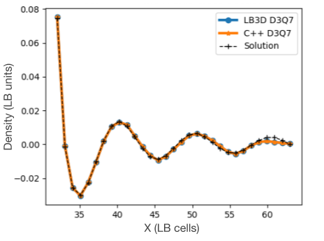
Figure 6: Density profile along the positive $x$-semi-axis and comparison with the analytical solution for the spherical waves of Fig. 5.

If the equilibrium distribution functions $f_{i}^{eq}$ are chosen in such a way that $\Pi^{(0)}$ becomes diagonal,

$$\Pi^{(0)}=\begin{bmatrix}p_{1}&0\\ 0&p_{1}\end{bmatrix}\quad\mbox{,}\quad\nabla\cdot\Pi^{(0)}=\nabla p_{1}\quad,$$ (67)

taking divergence on both sides of (65b) and using (67) and (65b) show us that the pressure fulfills

$$\partialderivative[2]{\rho_{1}}{t}+\nabla^{2}\rho_{1}=0\quad.$$ (68)

We can diagonalize $\Pi^{(0)}$ by choosing a velocity set $\vec{v}_{i}$ with weights $w_{i}$ such that

$$\sum_{i}w_{i}=1\quad,\quad\sum_{i}w_{i}v_{i\alpha}v_{i\beta}=c_{s}^{2}\delta_{\alpha\beta}$$ (69)

$$\sum_{i}\omega_{i}v_{i\alpha}=\sum_{i}\omega_{i}v_{i\alpha}v_{i\beta}v_{i\gamma}=0\quad,$$ (70)

where $v_{i\alpha}$ is the $\alpha-$th component ($\alpha\in x,y,z$) of $\vec{v}_{i}$ and $c_{s}^{2}$ is a constant. The equilibrium distribution functions

$$f_{i}^{eq}=\begin{cases}\rho_{1}(1+(1/c_{s}^{2})c_{0}^{2}(\omega_{0}-1))&\text{if}\quad i=0\\ (1/c_{s}^{2})\omega_{i}(c_{0}^{2}\rho_{1}+\vec{v}_{i}\cdot\vec{J}_{1})&\text{if}\quad i\neq 0\end{cases}\quad$$ (71)

make $\Pi^{(0)}$ diagonal (Eq. (67)), as desired Mendoza and Muñoz (2008). Here, $c_{s}$ is the speed of sound and $w_{0}$ is the weight associated with the null vector $\vec{v}_{0}=(0,0)$. Examples are D2Q5, D2Q9 and D3Q19 with $c_{s}^{2}=1/3$, and D3Q7, with $c_{s}^{2}=1/4$ (Fig. 4). The method has been extended to curvilinear cells and has been employed to simulate the normal modes in trumpets and even in the human Cochlea Velasco et al. (2019).

Boundary conditions, like a vibrating wall at $x_{0}=0$, can be set, first, by computing the equilibrium functions $f_{i}^{eq}$ with the desired value $\rho_{1}(x_{0}=0,y,z)=\rho_{a}\sin(\omega t)$ for the density (whereas $\vec{J}_{1}$ is computed from Eq. (62), as usual) and, next, by overwriting $f_{i}^{\rm new}$ with that equilibrium value. This operation, which we call imposing fields, is performed after collision and before advection, i.e.

$$f_{i}^{\rm new}(\vec{x},t)=f_{i}^{eq}\left(\rho_{1}(x_{0}=0,y,z),\vec{J}(\vec{x},t)\right)\quad.$$ (72)

The same procedure is employed to set the initial conditions. Other boundary conditions, like partially absorbing walls at $x_{n}=Lx-1$ with $Lx$ the length of the simulation domain in $x$ direction, are set by performing a bounce-back step (instead of the usual collision),

$$f_{i}(\vec{x}_{n},t_{n+1})=\Phi f_{j}(\vec{x}_{n},t_{n})\quad,$$ (73)

where $j$ is the index satisfying $\vec{v}_{j}=-\vec{v}_{i}$ and $\Phi\in[0,1)$ is a damping factor, which we set as $\Phi=0.99$. Finally, the results are plotted from the values $f_{i}^{\rm new}$ after imposing fields and before advection.

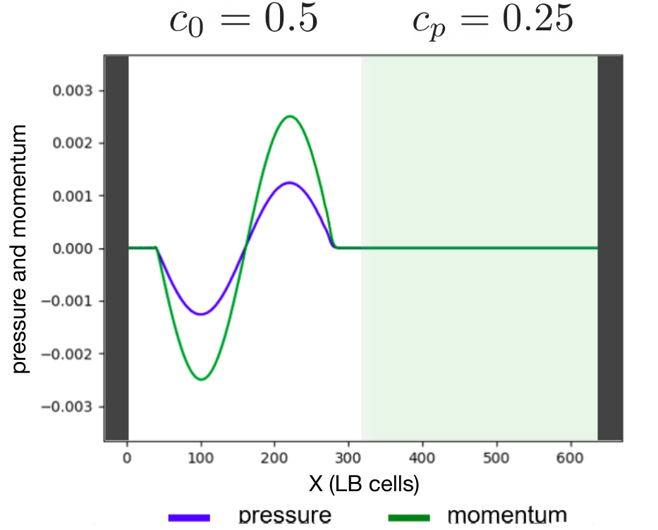
Figure 7: Incident waves in LBM.

Figure 8: Three-dimensional density map and mesh for the immersed sphere in LB3D.

The described LBM for waves was implemented in 2D on a self-developed C++ code (available in Supplementary material Code_2D_C++.zip and Gihub MyC (2024)), while for 3D simulations, the software 3nskog was modified to include this LB model as an additional feature. A first numerical test to validate the code was to simulate the density field in 3D produced by an oscillating point source at the origin, described by the inhomogeneous wave equation

$$\nabla^{2}\rho-\frac{1}{c^{2}}\frac{\partial^{2}\rho}{\partial t^{2}}=\delta(\vec{x}-\vec{x}^{\prime})\rho_{0}\sin(\omega t)\quad,$$ (74)

with $\omega$ the angular frequency. The solution is found through Green’s functions (Jackson, 1999, Sec. 6.4) and takes the form

$$\rho(\vec{x},t)=\frac{\rho_{0}\sin(\omega t-kr)}{4\pi kr}\quad,$$ (75)

where $r=|\vec{x}-\vec{x}^{\prime}|$ is the distance from the source position to the measurement point $\vec{x}$. Because the source term of (74) is proportional to $\sin(\omega t)$, the initial condition $\rho_{1}(x,t=0)=0$ everywhere coincides with the source and will not cause numerical instabilities. Figs. 5 and 6 show a good agreement between the analytical solution (75) and the 3D implementation and on a cubic domain of $64\times 64\times 64$ lattice cells.

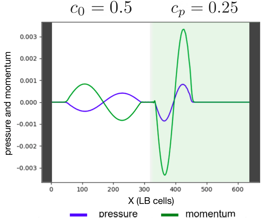
Figure 9: Reflected and transmitted waves in LBM.

A relevant test for our application is the simulation of an interface between two media with different sound speeds $c_{0}$ and $c_{p}$ The interface is modeled just by setting a smooth change in the speed of sound along the $x$ axis (to avoid numerical instabilities),

$$c(x)=\frac{c_{p}-c_{0}}{2}\tanh{\left(\frac{x-L_{x}/2}{w}\right)}+\frac{c_{p}+c_{0}}{2}\quad,$$ (76)

with $c_{0}=0.5$ and $c_{p}=0.25$, as shown in Figs. 7 and 9. This kind of boundary condition generates a typical refraction of waves entering in two media, which is sufficient to reproduce the Gor’kov force. By setting a traveling pulse as the initial condition, one expects that both pressure and the normal velocity must be continuous at the interface, i.e. that $p_{1,I}+p_{1,R}=p_{1,T}$ and $u_{1x,I}+u_{1x,R}=u_{1x,T}$, with $u_{1x}$ the $x$ component of the velocity and the subindexes $I$,$R$ and $T$ representing the incident, reflected and transmitted values at the interface, respectively. By simulating the interface in a domain of $Lx=$ cells, we obtain that those continuity conditions are fulfilled with 1% accuracy.

VI Wave-particle interaction and interpolation

To describe the wave-particle interaction in our LBM scheme it is useful to write the acoustic radiation force (14) in terms of the quantities $\vec{J}_{1}=\rho_{0}\vec{u}_{1}$ and $\rho_{1}=p_{1}/c_{0}^{2}$ that are computed by the LBM for waves, that is

$$\langle F_{i}\rangle=-\frac{1}{\rho_{0}}\oint\left\langle\left(-\frac{J_{1}^{2}}{2}+\frac{\rho_{1}^{2}c_{0}^{2}}{2}\right)\delta_{ij}+J_{1i}J_{1j}\right\rangle dS_{j}\quad.$$ (77)

This expression seems to be just a function of the density $\rho_{0}$ and the speed of sound $c_{0}$ in the fluid, but the values $\vec{J}_{1}$ and $\rho_{1}$ depend on the way the interface is modeled. The boundary conditions for the acoustic wave at the interface are that the pressure $p_{1}$ and the normal velocity $\vec{u}_{1}\cdot\hat{n}$ (with $\hat{n}$ a vector normal to the surface) must be continuous. Those conditions are equivalent to

$$\rho_{1}^{(0)}c_{0}^{2}=\rho_{1}^{(p)}c_{p}^{2}\quad,\quad\frac{\vec{J}_{1}^{(0)}\cdot\hat{n}}{\rho_{0}^{(0)}}=\frac{\vec{J}_{1}^{(p)}\cdot\hat{n}}{\rho_{0}^{(p)}}\quad,$$ (78)

where the superscripts $(0)$ and $(p)$ identify the values of the fields $\vec{J}_{1}$ and $\rho_{1}$ at the fluid side and the object side, respectively.

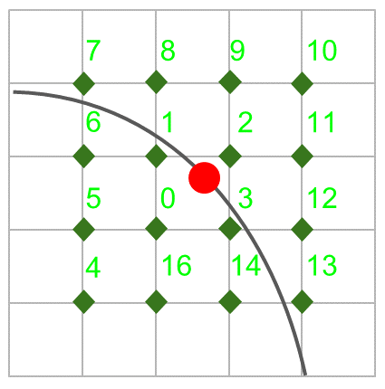
Figure 10: Kernel interpolation scheme.

For the sake of ease, we choose a much simpler approach, assuming that mean densities on both media are equal ($\rho_{0}^{(0)}=\rho_{0}^{(p)}$) and that only the speed of sound changes, as

$$c(\vec{r})=c_{0}-\frac{c_{0}-c_{p}}{2}\left(1-\tanh{\left(\frac{|\vec{r}-\vec{r}_{0}|^{2}-R_{p}^{2}}{d}\right)}\right)\quad,$$ (79)

where $\vec{r}=(x,y,z)$, $\vec{r}^{\prime}=(x_{0},y_{0},z_{0})$ and $d$ is the square thickness of the interface, which was set as $d=4$ for our simulations. In Fig. 8 a three-dimensional density map of function (79) is illustrated. This approach is enough to verify that our procedure reproduces Gor’kov and Wei theoretical expressions for the acoustic radiation force on a sphere (3D) and a disk (2D), as we will see in the following Section.

The acoustic radiation force (77) is computed by dividing the object’s boundary into $N$ surface elements (which are segments in 2D and triangles in 3D) and by computing the normal vector $\hat{n}$ and the fields $\rho_{1}$ and $\vec{J}_{1}$ at the center $\vec{R}_{k}$ of each element, but those points do not usually coincide with the nodes $\vec{R}^{\text{LB}}$ of the LB mesh (Fig. 10). To calculate the fields at $\vec{R}_{k}$ we use kernel interpolation Mühlenstädt and Kuhnt (2011); Roma et al. (1999), expressing those fields as a weighted sum on the neighboring cells,

$$\rho_{\text{I}}(\vec{R}_{k}) =\sum_{l}\rho(\vec{R}_{l}^{\text{LB}})\delta(|\vec{R}_{l}^{\text{LB}}-\vec{R}_{k}|)\quad,$$ (80)

$$\vec{J}_{\text{I}}(\vec{R}_{k}) =\sum_{l}\vec{J}(\vec{R}_{k})\delta(|\vec{R}_{l}^{\text{LB}}-\vec{R}_{k}|)\quad,$$ (81)

with weights depending on the distance $r=|\vec{R}_{l}^{\text{LB}}-\vec{R}_{k}|$ through the kernel function Favier et al. (2014)

$$\delta(r)=\begin{cases}\frac{1}{6}\left(5-3|r|-\sqrt{-3(1-|r|)^{2}+1}\right)&|r|\in\left[\frac{1}{2},\frac{3}{2}\right]\\ \frac{1}{3}\left(1+\sqrt{-3r^{2}+1}\right)&|r|\leq\frac{1}{2}\\ 0&\text{elsewhere}\end{cases}\quad.$$ (82)

Parameter	Value
$c_{p}$	0.25
$c_{0}$	0.24
$p_{0}$	1.00
$\lambda$	500
$R_{p}$	10
$x$	$\lambda/8$

Table 1: Default fixed values for the relevant quantities of the acoustic radiation force.

VII Results and discussion

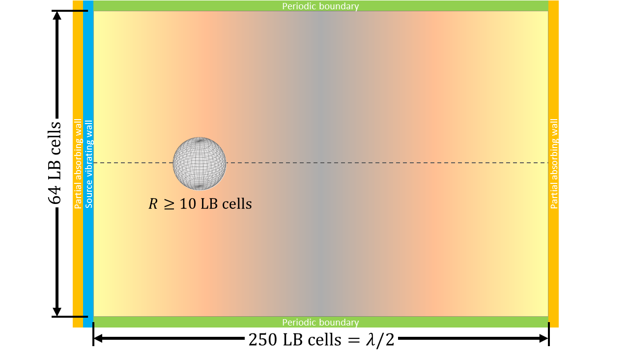
Figure 11: Simulation’s domain and setup.

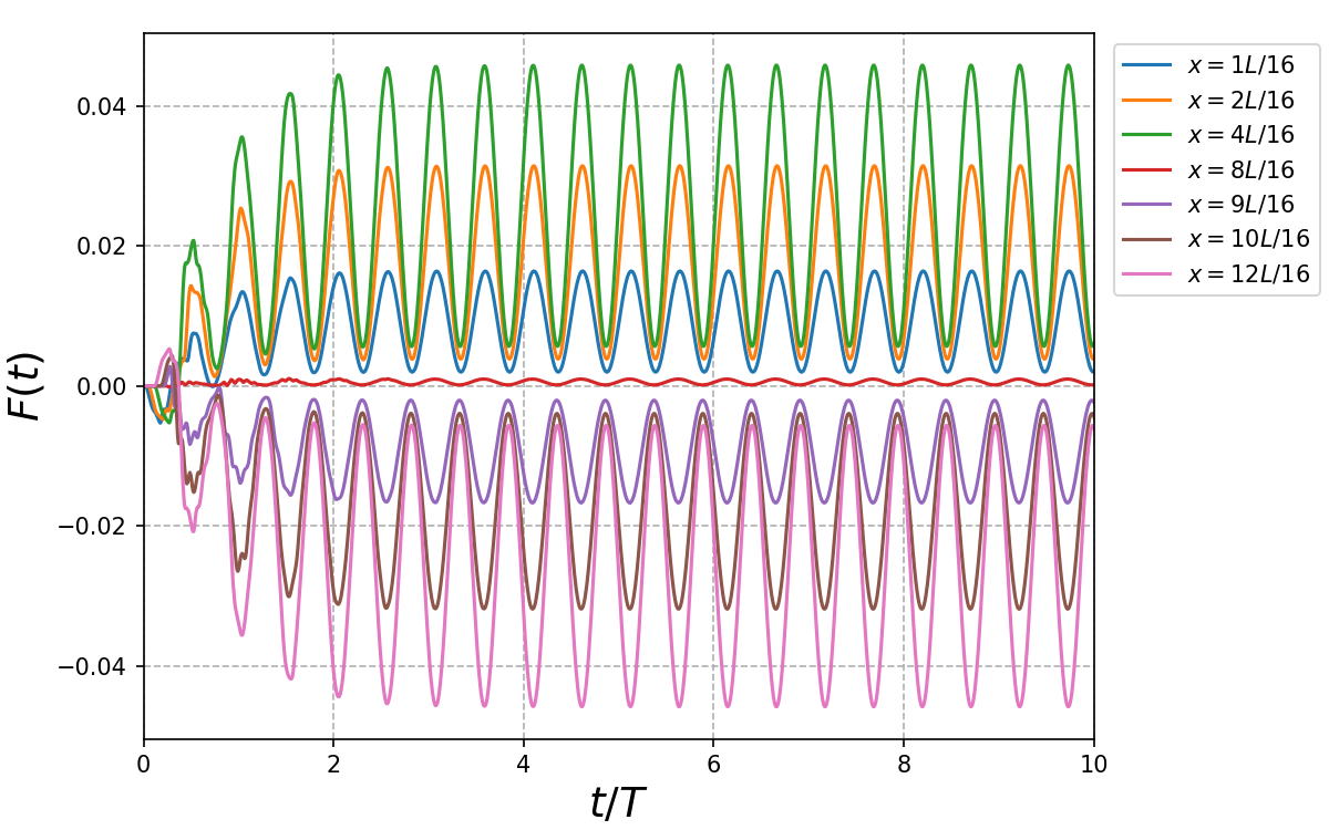
Figure 12: Different curves of the time-dependent force varying the object’s axial position.

To compute the acoustic radiation force on a sphere and a disk and to compare the results with the Gor’kov and Wei solutions, respectively, the simulation domain is a box with $L_{y}=L_{z}=64$ cells along $y$ and $z$ axis in 3D and $L_{y}=64$ cells in 2D. The length $Lx$ along the $x$ axis is chosen such that $Lx=\lambda/2+3$, with $100\leq\lambda\leq 2560$ the wavelength in cell units (Fig. 11). The object, a sphere or a disk of radius $R_{p}$, is placed with its center at $\vec{r}_{0}=(x_{0},L_{y}/2,L_{z}/2)$ and the speed of sound was chosen at every cell by using (79). The default values for the mean density $\rho_{0}$, the wavelenght $\lambda$, the object’s radius $R_{p}$, the speed of sound in the fluid $c_{0}$ and in the object, $c_{p}$, are listed in Table 1. The left wall, chosen as source, is built with two extra sheets: one partial absorbing wall at $x=0$ and one source of plane waves at $x=1$, forcing the density to oscillate as $\rho_{a}\sin(\omega t)$ (Eq. (72)). The right wall, at $x=L_{x}+2$ (i.e. the last cells in the $x$ axis) is chosen as a partially absorbing reflector (Eq. (73)). In addition, periodic boundary conditions are set on $y$ and $z$ directions. The result is a standing wave with a single nodal plane at $x=L_{x}/2+1$.

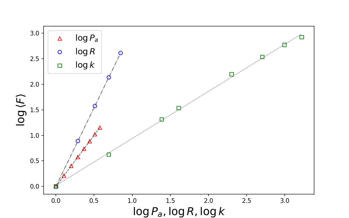
Figure 13: Acoustic radiation force of the sphere (3D) for several pressure amplitudes $P_{a}$, sphere’s radii $R_{p}$ and wave numbers $k$.

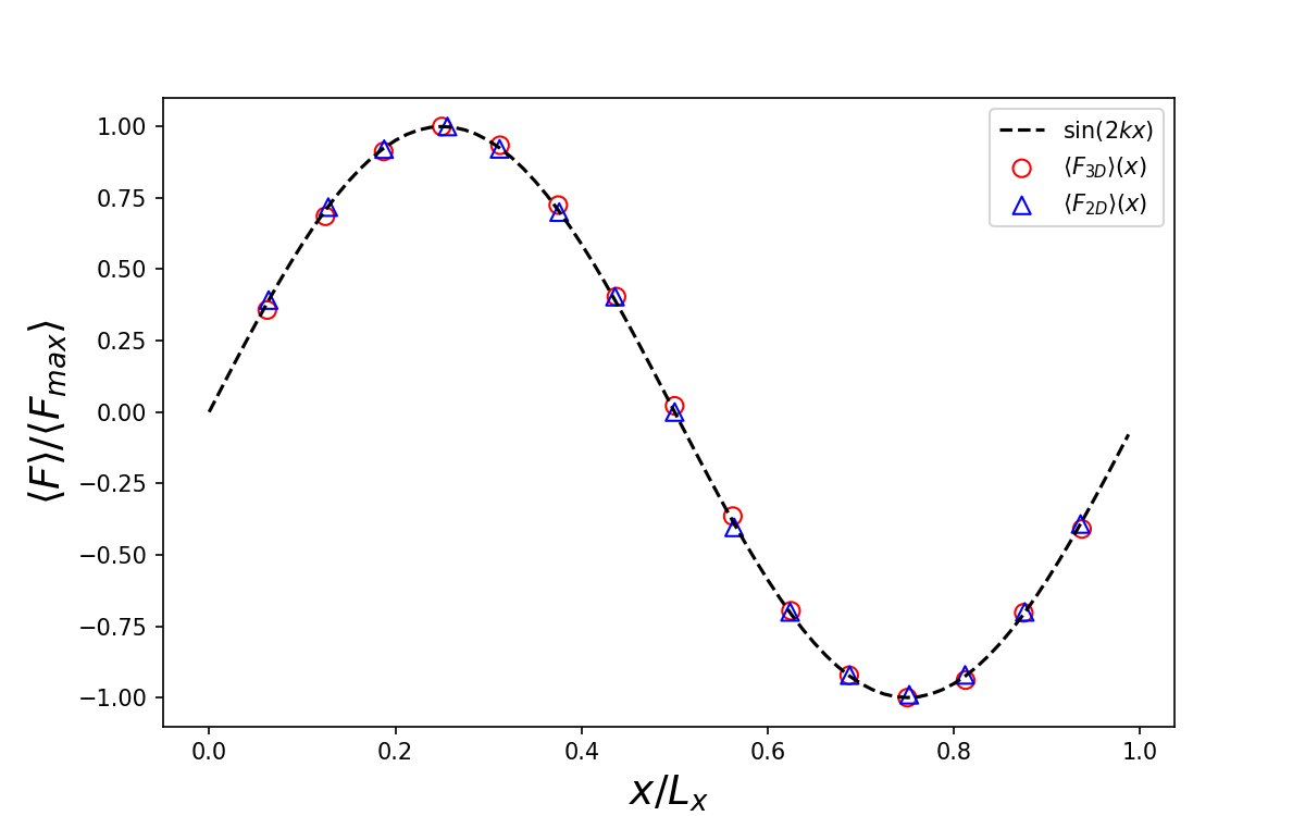
Figure 14: Acoustic radiation forces in 2D and 3D along the $x$ axis showing a $\sin 2kx$ dependence.

Each simulation runs for more than $10T$ time steps, with $T=\lambda/c_{0}$ the period of acoustic oscillations. The acoustic radiation force is measured at every time step using (77), giving us a curve of $F_{x}(t)$ vs. time that stabilizes after around ten oscillations. Once it stabilizes, $\left<F_{x}\right>$ is measured as that signal’s average (Fig. 12).

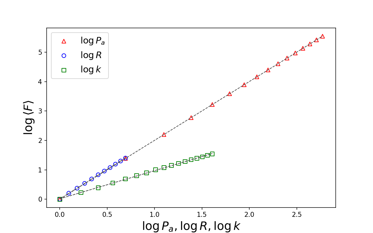
Figure 15: Acoustic radiation force of the disk (2D) for several pressure amplitudes $P_{a}$, disk’s radii $R_{p}$ and wave numbers $k$.

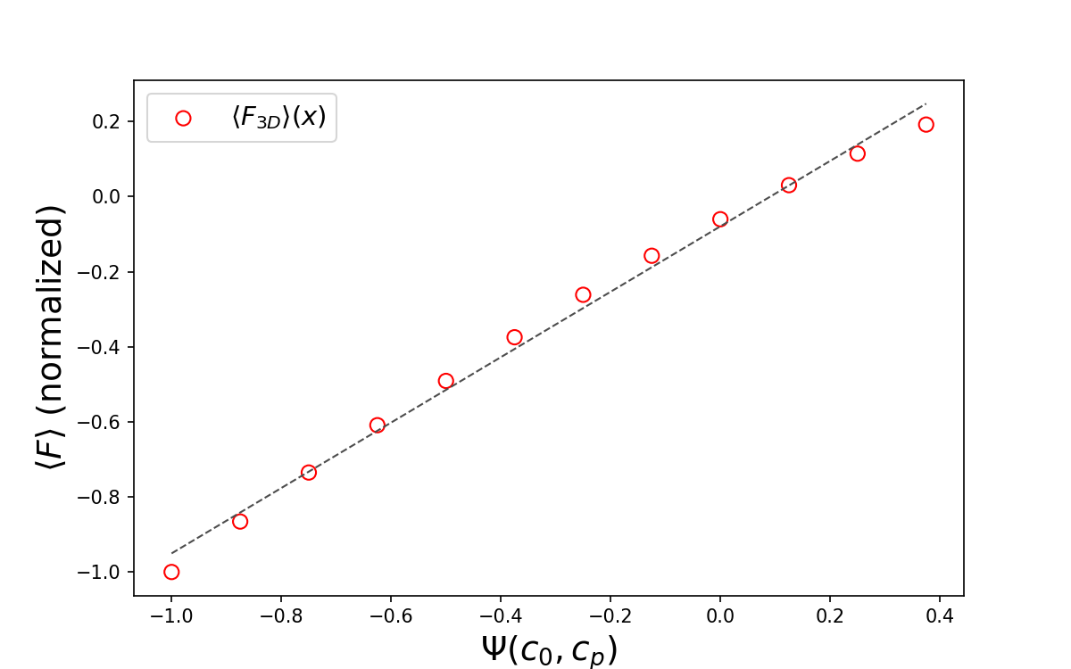
Figure 16: Acoustic radiation force of the sphere (3D) for several values of the contrast factor $\Psi$ (Eq. (84)).

Parameter	Expected	Measured	Rel. Err. (%)
$P_{a}$	$2.0000$	$1.9999$	$10^{-13}$
$k$	$1.0000$	$0.9222$	$7.7783$
$R_{p}$	$3.0000$	$3.0814$	$2.7119$

Table 2: Power law exponents comparison in 3D.

The measurements are compared with the theoretical expressions (41) and (60) for the sphere and the disk, respectively, with equal mean densities for the fluid and the object, that we rewrote as

$$\langle F_{x}\rangle_{\text{3D}}=-\frac{\pi R_{p}^{3}P_{a}^{2}k}{3\rho_{0}}\Psi(c_{0},c_{p})\sin 2kx\mbox{ ,}$$ (83a)

$$\langle F_{x}\rangle_{\text{2D}}=-\frac{\pi R_{p}^{2}P_{a}^{2}k}{4\rho_{0}}\Psi(c_{0},c_{p})\sin 2kx\mbox{ .}$$ (83b)

Hereby we have defined the contrast factor $\Psi(c_{0},c_{p})$ as

$$\Psi(c_{0},c_{p})=\frac{1}{c_{0}^{2}}-\frac{1}{c_{p}^{2}}\quad.$$ (84)

Simulations were performed by varying one at a time the physical parameters the force depends on, whereas the other parameters remain fixed to default values (Tab. 1). The varied parameters are the axial position of the object $x$, the pressure acoustic amplitude $P_{a}$, the radius of the object $R_{p}$ and the wave number $k=2\pi/\lambda$. The contrast factor $\Psi(c_{0},c_{p})$ is also properly changed to find out its linear relationship with the force.

Figure 14 shows that the simulated force follows a behavior proportional to $\sin(2kx)$ for both 3D and 2D cases, being the force zero when the object is at $x=8L/16=\lambda/4$ where the node is (see Fig. 12). When $\Psi(c_{0},c_{p})>0$, this is a confining force at the nodal plane. Concerning $R_{p}$, $k$ and $P_{a}$, we can see from (83) that a power law relationship with the force is expected for each one of them. Figures 13 and 15 show that this is the case for both the sphere and the disk, with all correlation coefficients close to $0.99$. The measured exponents for those power laws show an excellent agreement with the expected values (Tabs. 2 and 3).

Regarding the contrast factor, we expect a linear relationship between $\left<F_{x}\right>$ and $\Psi(c_{0},c_{p})$ (Eq. (83)). For this test, the speed of sound for the fluid was set to $c_{0}=0.25$, whereas $c_{p}$ was adjusted so that the factor $\Psi$ changes uniformly. Figure 17 confirms that linear behavior for both the sphere and the disk, with $R^{2}=0.994$ and $R^{2}=0.999$ for the 3D and 2D cases, respectively.

Summarizing, our simulations show that the proposed method to compute the acoustic radiation force reproduces with great precision both the theoretical expressions by Gor’kov and Wei.

VIII Conclusions

We employed a lattice Boltzmann model that reproduces the wave equation to compute the acoustic radiation force on a compressible object immersed in an inviscid fluid. Instead of simulating the full Navier-Stokes equations (NSE), our proposal relies on the solution of the wave equation from which, via an interpolation scheme, the first order perturbations in the velocity $\vec{u}_{1}$ and the pressure $p_{1}$ are computed on the object’s surface and, from them, the force. We tested our novel numerical approach by computing the acoustic radiation force on a disk (in 2D) and on a sphere (in 3D) produced by a standing wave with a single nodal plane, with wavelengths much larger than the particle size. The method reproduces with excellent accuracy the theoretical predictions by Gor’kov Gor’kov (1962) and Wei et al. Wei et al. (2004) for the sphere and the disk, respectively, in all studied cases. The procedure to compute the acoustic radiation force from the fields $p_{1}$ and $\vec{u}_{1}$ is general, and can be performed with any numerical method for solving the wave equation.

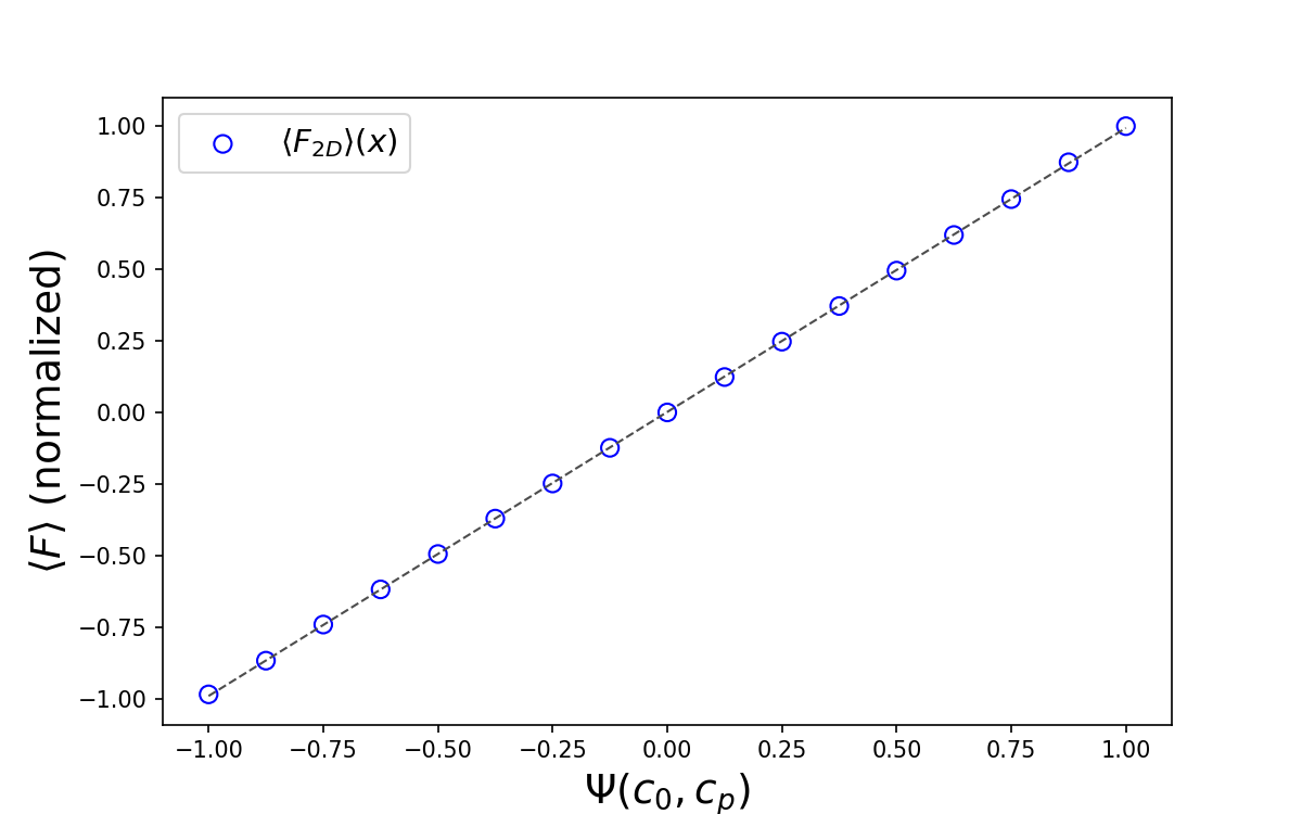
Figure 17: Acoustic radiation force of the disk (2D) for several values of the contrast factor $\Psi$ (Eq. (84)).

Parameter	Expected	Measured	Rel. Err. (%)
$P_{a}$	$2.0000$	$1.9994$	$0.0302$
$k$	$1.0000$	$0.9569$	$4.3108$
$R_{p}$	$2.0000$	$2.0127$	$0.6373$

Table 3: Power law exponents comparison in 2D.

One of the advantages of our numerical approach is that it computes $p_{1}$ and $\vec{u}_{1}$, with second order accuracy, and hence it needs fewer cells to compute the acoustic radiation force than other methods simulating the full Navier-Stokes equations. Actually, widely used LBMs for fluids compute with second order accuracy the zeroth order density and velocity fields and, with only first order accuracy the perturbative fields $p_{1}$ and $\vec{u}_{1}$. Accordingly, our method obtains excellent results by using grids of just $250\times 64$ cells for the 2D case and $250\times 64\times 64$ for the 3D one, whereas a previous work using a LBM for the full NSE Cosgrove et al. (2004) requires $600\times 600$ cells to obtain reliable results in 2D. Our method is also very fast. When implemented in C++ it takes up to $3$ minutes on a laptop with a single Intel Core-i5 processor to compute the acoustic radiation force on a disk with the simulation domain described above. Similarly, when implemented in our 3D solver 3nskog it takes no longer than $30$ minutes by running on four processors to compute the acoustic radiation force on a sphere.

The values of $p_{1}$ and $\vec{u}_{1}$ on the object’s surface and the acoustic radiation force computed from them rely on the boundary conditions employed to model the object itself. For simplicity, in our tests we used just a smooth change in the speed of sound when crossing from the fluid to the object, assuming that the mean densities in both media are equal. On the one hand, such an approximation can be enough for nearly buoyant particles. On the other hand, this strategy assures that both the pressure and the normal velocity are continuous at the interface. The actual boundary conditions (Eq. (78)) relate both the momenta and the densities on both sides of the interface. Finding the way to implement those more general boundary conditions in our LBM will be an interesting subject for future work.

The proposed approach is completely general and can be used to compute the acoustic radiation force on an object of any shape in 2D or 3D, like microbots or self-assembled microswimmers. Moreover, it can be coupled with standard numerical integration algorithms to compute the three-dimensional movement of such objects due to acoustic radiation forces (see Supplementary Material Movie.gif). This opens a broad spectrum of future applications in the acoustic manipulation of many objects. In addition, being able to have both waves and fluids in the same LBM code allows to simulate multi-physics applications efficiently. For example, the method could be employed for the study of systems like acoustic-driven bubbles or reactions among fluids pushed by micro-particles of solid catalyst driven by acoustic forces, just to mention a few. All those are interesting subjects for future research.

The present work introduces a fast and accurate numerical procedure to compute the acoustic radiation force on an object immersed in an inviscid fluid. The proposed procedure shows to be a promising tool for the study of the many phenomena in medicine and engineering where that force plays a relevant role.

IX Acknowledgments

We acknowledge financial support from the Bavarian University Center for Latin America (BAYLAT). Also, we thank the 3nskog developer team, in particular Johannes Hielscher and Dr. Othmane Auoane, whose advice and technical support were fundamental to develop the simulation code.

Appendix A Deducting the second order acoustic radiation force

By replacing the second order expansion written in (12) into the mass (Eq. (1)) and momentum (Eq. (2)) conservation law, using Eq. (7) and taking the second order terms only, we obtain

$$\frac{\partial\rho_{2}}{\partial t}+\rho_{0}\nabla\cdot\vec{u}_{2}+\nabla\cdot(\rho_{1}\vec{u}_{1})=0\quad,$$ (85a)

$$\rho_{0}\frac{\partial\vec{u}_{2}}{\partial t}+\rho_{1}\frac{\partial\vec{u}_{1}}{\partial t}+\nabla p_{2}+\rho_{0}(\vec{u}_{1}\cdot\nabla)\vec{u}_{1}=0\quad.$$ (85b)

The last term of the left side of Eq. (85b) can be rewritten by using the following mathematical property,

$$\frac{1}{2}\nabla(\vec{u}_{1}\cdot\vec{u}_{1})=(\vec{u}_{1}\cdot\nabla)\vec{u}_{1}+\vec{u}_{1}\times(\nabla\times\vec{u}_{1})\quad,$$ (86)

where the term $\vec{u}_{1}\times(\nabla\times\vec{u}_{1})=0$, because the flow is irrotational. Then (85b) becomes

$$\rho_{0}\frac{\partial\vec{u}_{2}}{\partial t}+\rho_{1}\frac{\partial\vec{u}_{1}}{\partial t}+\nabla p_{2}+\frac{\rho_{0}}{2}\nabla(u_{1}^{2})=0\quad.$$ (87)

By using Eqns. (6) and (7a), the second term of the left hand side may be written as

$$\rho_{0}\frac{\partial\vec{u}_{2}}{\partial t}-\frac{p_{1}}{\rho_{0}c^{2}}\nabla p_{1}+\nabla p_{2}+\frac{\rho_{0}}{2}\nabla(u_{1}^{2})=0$$ (88)

and using the product derivative property for gradients, we end up with

$$\rho_{0}\frac{\partial\vec{u}_{2}}{\partial t}+\nabla p_{2}=\frac{1}{2\rho_{0}c_{0}^{2}}\nabla(p_{1}^{2})-\frac{\rho_{0}}{2}\nabla(u_{1}^{2})\quad.$$ (89)

Because we are interested in writing the total velocity and pressure fields in terms of only first order terms, let us add Eq. (7a) as a null term such that, by using 12b and (12c) we have

$$\rho_{0}\frac{\partial\vec{u}_{2}}{\partial t}+\rho_{0}\frac{\partial\vec{u}_{1}}{\partial t}+\nabla p_{2}+\nabla p_{1} =\frac{1}{2\rho_{0}c_{0}^{2}}\nabla(p_{1}^{2})-\frac{\rho_{0}}{2}\nabla(u_{1}^{2})\,,$$

$$\rho_{0}\frac{\partial\vec{u}}{\partial t}+\nabla(P-p_{0}) =\nabla\left(\frac{1}{2\rho_{0}c^{2}}p_{1}^{2}-\frac{\rho_{0}}{2}u_{1}^{2}\right)\quad.$$ (90)

By using (9) we end up with a total non-static pressure

$$\nabla(P-p_{0})=\nabla\left(\frac{p_{1}^{2}}{2\rho_{0}c_{0}^{2}}-\frac{\rho_{0}}{2}u_{1}^{2}-\rho_{0}\frac{\partial\phi}{\partial t}\right)$$ (91)

written also in (13).

Appendix B Incident, scattered and interference terms

With the velocity potential divided into an incident and a scattered field, the average force Eq. (4) has three contributions. The first one, due to $\phi_{\text{in}}$ only,

$$\langle F_{i,\textsc{in}}\rangle =-\rho_{0}\oint\bigg{\langle}\left(-\frac{\rho_{0}}{2}|\nabla\phi_{\text{in}}|^{2}+\frac{\rho_{0}}{2c_{0}^{2}}\left[\frac{\partial\phi_{\text{in}}}{\partial t}\right]^{2}\right)\delta_{ij}$$

$$+\rho_{0}\partial_{i}\phi_{\text{in}}\partial_{j}\phi_{\text{in}}\bigg{\rangle}dS_{i}$$ (92)

should be zero because the incident field (which is the solution in the absence of the object) does not receive any physical effect from the particle. In the case of plane waves, the incident field $\phi_{\text{in}}=\phi_{0}\cos(\vec{k}\cdot\vec{r}-\omega t)$ is spatially homogeneous, implying a symmetry over the surface, and the closed integral will yield zero (Manneberg, 2009,  p.79)(Bruus, 2012b,  p.). The other two contributions containing information about the scattered wave are

$$\langle F_{i,\textsc{sc}}\rangle =-\rho_{0}\oint\bigg{\langle}\left(-\frac{\rho_{0}}{2}|\nabla\phi_{\text{sc}}|^{2}+\frac{\rho_{0}}{2c_{0}^{2}}\left[\frac{\partial\phi_{\text{sc}}}{\partial t}\right]^{2}\right)\delta_{ij}$$

$$+\rho_{0}\partial_{i}\phi_{\text{sc}}\partial_{j}\phi_{\text{sc}}\bigg{\rangle}dS_{i}$$ (93)

and

$$\langle F_{i,\textsc{in-sc}}\rangle =-\rho_{0}\oint\bigg{\langle}\bigg{(}-\rho_{0}\nabla\phi_{\text{in}}\cdot\nabla\phi_{\text{sc}}+$$

$$\frac{\rho_{0}}{c_{0}^{2}}\bigg{[}\frac{\partial\phi_{\text{in}}}{\partial t}\bigg{]}\bigg{[}\frac{\partial\phi_{\text{sc}}}{\partial t}\bigg{]}\bigg{)}\delta_{ij}+$$

$$\rho_{0}\partial_{i}\phi_{\text{in}}\partial_{j}\phi_{\text{sc}}+\rho_{0}\partial_{i}\phi_{\text{sc}}\partial_{j}\phi_{\text{in}}\bigg{\rangle}dS_{i}\quad.$$ (94)

The contribution $\langle F_{i,\textsc{sc}}\rangle$ is much smaller than the interference term $\langle F_{i,\textsc{in-sc}}\rangle$ because the scattering cross-section of a spherical particle is proportional to $(kR_{p})^{4}$, which is negligible due to $R_{p}\ll\lambda$, and because the scattered potential field solution is proportional to $R_{p}^{3}$, as will be shown later. Thus, the interference term (B) is the most relevant, and that is the one to be developed next (Manneberg, 2009,  p.79). By using (9)

$$\nabla\phi_{in}\cdot\nabla\phi_{sc}=\vec{u}_{in}\cdot\vec{u}_{sc}\quad,$$ (95a)

$$\frac{\rho_{0}}{c_{0}^{2}}\frac{\partial\phi_{in}}{\partial t}\frac{\partial\phi_{sc}}{\partial t}=\frac{c_{0}^{2}}{\rho_{0}}\rho_{in}\rho_{sc}\quad,\text{ and}$$ (95b)

$$\partial_{i}\phi_{\text{in}}\partial_{j}\phi_{\text{sc}}=u_{\text{in}}^{i}u_{\text{sc}}^{j}$$ (95c)

the interference term becomes

$$\langle F_{i,\textsc{in-sc}}\rangle =-\rho_{0}\oint\bigg{\langle}\left(-\rho_{0}\vec{u}_{\text{in}}\cdot\vec{u}_{\text{sc}}+\frac{c_{0}^{2}}{\rho_{0}}\rho_{in}\rho_{sc}\right)\delta_{ij}$$

$$+\rho_{0}u_{\text{in}}^{i}u_{\text{sc}}^{j}+\rho_{0}u_{\text{sc}}^{i}u_{\text{in}}^{j}\bigg{\rangle}dS_{i}\quad.$$ (96)

By using Gauss’ theorem, the surface integral transforms into a volume integral,

$$\langle F_{i,\textsc{in-sc}}\rangle=-\rho_{0}\int\bigg{\langle}\bigg{(}-\rho_{0}(\partial_{i}u_{\text{in}}^{m})u_{\text{sc}}^{m}-\rho_{0}(\partial_{i}u_{\text{sc}}^{m})u_{\text{in}}^{m}+$$

$$\frac{c_{0}^{2}}{\rho_{0}}\partial_{i}\rho_{in}\rho_{sc}+\frac{c_{0}^{2}}{\rho_{0}}\rho_{in}\partial_{i}\rho_{sc}\bigg{)}\delta_{ij}+\rho_{0}(\partial_{i}u_{\text{in}}^{i})u_{\text{sc}}^{j}$$

$$+\rho_{0}u_{\text{in}}^{i}(\partial_{i}u_{\text{sc}}^{j})+\rho_{0}(\partial_{i}u_{\text{sc}}^{i})u_{\text{in}}^{j}+\rho_{0}u_{\text{sc}}^{i}(\partial_{i}u_{\text{in}}^{j})\bigg{\rangle}dV\quad.$$ (97)

The first two terms may be rewritten as

$$(\partial_{i}u_{\text{in}}^{m})u_{\text{sc}}^{m}+(\partial_{i}u_{\text{sc}}^{m})u_{\text{in}}^{m} =(\partial_{i}\partial_{m}\phi_{\text{in}})u_{\text{sc}}^{m}+(\partial_{i}\partial_{m}\phi_{\text{sc}})u_{\text{in}}^{m}\,,$$

$$=(\partial_{m}\partial_{i}\phi_{\text{in}})u_{\text{sc}}^{m}+(\partial_{m}\partial_{i}\phi_{\text{sc}})u_{\text{in}}^{m}\,,$$

$$=(\partial_{m}u_{\text{in}}^{i})u_{\text{sc}}^{m}+(\partial_{m}u_{\text{sc}}^{i})u_{\text{in}}^{m}$$ (98)

and the interference term simplifies to

$$\langle F_{i,\textsc{in-sc}}\rangle =-\rho_{0}\int\bigg{\langle}\frac{c_{0}^{2}}{\rho_{0}}\partial_{j}\rho_{in}\rho_{sc}+\frac{c_{0}^{2}}{\rho_{0}}\rho_{in}\partial_{j}\rho_{sc}$$

$$+\rho_{0}(\partial_{i}u_{\text{in}}^{i})u_{\text{sc}}^{j}+\rho_{0}(\partial_{i}u_{\text{sc}}^{i})u_{\text{in}}^{j}\bigg{\rangle}dV\quad.$$ (99)

Now, by using (7) for the incident and scattered fields on all terms but the last one, we obtain

$$\langle F_{i,\textsc{in-sc}}\rangle=-\rho_{0}\int\bigg{\langle}-\frac{\partial u_{\text{in}}^{j}}{\partial t}\rho_{sc}-\frac{\partial u_{\text{sc}}^{j}}{\partial t}\rho_{in}-\frac{\partial\rho_{\text{in}}}{\partial t}u_{\text{sc}}^{j}$$

$$+\rho_{0}(\partial_{i}u_{\text{sc}}^{i})u_{\text{in}}^{j}\bigg{\rangle}dV-$$

$$\int\bigg{\langle}-\frac{\partial u_{\text{in}}^{j}}{\partial t}\rho_{sc}-\frac{\partial}{\partial t}(u_{\text{sc}}^{j}\rho_{in})+\rho_{0}(\partial_{i}u_{\text{sc}}^{i})u_{\text{in}}^{j}\bigg{\rangle}dV\quad.$$ (100)

Since

$$-\frac{\partial u_{\text{in}}^{j}}{\partial t}\rho_{sc}=-\frac{\partial}{\partial t}(u_{\text{in}}^{j}\rho_{sc})+u_{\text{in}}^{j}\frac{\partial\rho_{sc}}{\partial t}$$ (101)

the averaged force simplifies to

$$\langle F_{i,\textsc{in-sc}}\rangle =-\rho_{0}\int\bigg{\langle}-\frac{\partial}{\partial t}(u_{\text{sc}}^{j}\rho_{in}+u_{\text{in}}^{j}\rho_{sc})+$$

$$u_{\text{in}}^{j}\frac{\partial\rho_{sc}}{\partial t}+\rho_{0}(\partial_{i}u_{\text{sc}}^{i})u_{\text{in}}^{j}\bigg{\rangle}dV\quad.$$ (102)

Because the time-average of the time derivatives of any periodic function is identically zero, the force simplifies further to

$$\langle\vec{F}\rangle=-\rho_{0}\int\left\langle\vec{u}_{\text{in}}\left(\nabla^{2}\phi_{\text{sc}}-\frac{1}{c_{0}^{2}}\frac{\partial^{2}\phi_{\text{sc}}}{\partial t^{2}}\right)\right\rangle dV\quad.$$ (103)

Therefore, the time-averaged force on the small sphere can be found if we compute the scattered velocity potential $\phi_{sc}$.

Appendix C Integrating the acoustic radiation force to obtain the Gor’kov potential

With (24) and (35) it is now possible to write a particular solution for the scattered velocity potential previously defined in terms of $a(t^{\prime})$ and $\vec{A}(t^{\prime})$ (Eq. (III)). It becomes

$$\phi_{\text{sc}}(r,t)=-f_{1}\frac{R_{p}^{3}}{3\rho_{0}r}\dot{\rho_{\text{in}}}-f_{2}\frac{R_{p}^{3}}{2r^{2}}\nabla\cdot\left(\frac{\vec{u}_{\text{in}}}{r}\right)\mbox{ .}$$ (104)

this potential actually satisfies a non-homogeneous wave equation. By applying the D’Alembert operator, as it is done in (16), the following source is gathered

$$\nabla^{2}\phi_{\text{sc}}-\frac{1}{c_{0}^{2}}\frac{\partial^{2}\phi_{\text{sc}}}{\partial t^{2}}=f_{1}\frac{V_{p}}{\rho_{0}}\dot{\rho_{\text{in}}}\delta(\vec{r})+f_{2}\frac{3V_{p}}{2}\nabla\cdot\left(\vec{u}_{\text{in}}\delta(\vec{r})\right)$$ (105)

After plugging in (105) into (16), we have

$$\langle F_{i}\rangle=-V_{p}\int\left\langle f_{1}\dot{\rho_{\text{in}}}u_{\text{in}}^{i}\delta(\vec{r})+f_{2}\frac{3\rho_{0}}{2}u_{\text{in}}^{i}\partial_{k}(u_{\text{in}}^{k}\delta(\vec{r}))\right\rangle dV$$

$$=-f_{2}\frac{3\rho_{0}V_{p}}{2}\bigg{(}\oint\left\langle u_{\text{in}}^{i}u_{\text{in}}^{k}\delta(\vec{r})\right\rangle dS_{k}$$

$$-\int\left\langle(u_{\text{in}}^{k}\partial_{k})u_{\text{in}}^{i}\delta(\vec{r})\right\rangle dV\bigg{)}-f_{1}V_{p}\left\langle\frac{\partial\rho_{\text{in}}}{\partial t}u_{\text{in}}^{i}\right\rangle$$ (106)

Because the Dirac’s delta of the second term of does not contain the surface, the whole integrand is identically zero, leading to

$$\langle F_{i}\rangle=-f_{1}V_{p}\left\langle\frac{\partial\rho_{\text{in}}}{\partial t}u_{\text{in}}^{i}\right\rangle+f_{2}\frac{3\rho_{0}V_{p}}{2}\left\langle(u_{\text{in}}^{k}\partial_{k})u_{\text{in}}^{i}\right\rangle\mbox{ .}$$ (107)

As a final step, we can exchange the time derivative in the first term, because the derivative of the whole product is identically zero (just because the incident field oscillates harmonically); thus

$$\left\langle\frac{\partial\rho_{\text{in}}}{\partial t}u_{\text{in}}^{i}\right\rangle=\frac{1}{2\rho_{0}c_{o}^{2}}\left\langle\partial_{i}p_{\text{in}}^{2}\right\rangle\quad,$$ (108)

where (7) was considered. By using (86) in the second term of (107) and by replacing the previous result, the Gor’kov Force takes its definitive form,

$$\langle F_{i}\rangle=-\partial_{i}V_{p}\left(f_{1}\frac{1}{2\rho_{0}c_{0}^{2}}\langle p_{\text{in}}^{2}\rangle+f_{2}\frac{3\rho_{0}}{4}\langle u_{\text{in}}^{2}\rangle\right)=-\nabla U$$ (109)

written in (36).

References

- Mohanty et al. (2020) S. Mohanty, I. S. M. Khalil, and S. Misra, The Royal Society 476 (2020), 10.1098/rspa.2020.0621.
- Ahmed et al. (2021) D. Ahmed, A. Sukhov, D. Hauri, D. Rodrigue, G. Maranta, J. Harting, and B. J. Nelson, Nature Machine Intelligence 3, 116 (2021).
- Jinjie et al. (2009) S. Jinjie, A. Daniel, M. Xiaole, L. S.-C. Steven, L. Aitan, and H. T. Jun, Lab Chip 9, 2890 (2009).
- Marzo et al. (2015) A. Marzo, S. A. Seah, and B. W. D. et. al., Nature Communications 6 (2015), 10.1038/ncomms9661.
- Ashkin (1970) A. Ashkin, Phys. Rev. Lett. 24, 156 (1970).
- Gutsche et al. (2008) C. Gutsche, F. Kremer, M. Krüger, M. Rauscher, R. Weeber, and J. Harting, J. Chem. Phys. 129, 084902 (2008).
- Bruus (2006) H. Bruus, Theoretical microfuidics, 3rd ed., Vol. 6 (Lecture notes from Department of Micro and Nanotechnology, Technical University of Denmark, 2006).
- Ozcelik et al. (2018) A. Ozcelik, J. Rufo, and F. G. et. al., Nature Methods 15, 1021–1028 (2018).
- Ghanem et al. (2020) M. A. Ghanem, A. D. Maxwell, Y.-N. Wang, B. W. Cunitz, V. A. Khokhlova, O. A. Sapozhnikov, and M. R. Bailey, Proceedings of the National Academy of Sciences 117, 16848 (2020), https://www.pnas.org/doi/pdf/10.1073/pnas.2001779117 .
- Zhang et al. (2022) Z. Zhang, A. Sukhov, J. Harting, P. Malgaretti, and D. Ahmed, nature communications 13 (2022), 10.1038/s41467-022-35078-8.
- Andrade et al. (2018) M. A. B. Andrade, N. Pérez, and J. C. Adamowski, Brazilian Journal of Physics 48, 190–213 (2018).
- King (1934) L. V. King, Proc. R. Soc. Lond. A 147, 212–240 (1934).
- King (1935) L. V. King, Proc. R. Soc. Lond. A 153, 1–16 (1935).
- Gor’kov (1962) L. P. Gor’kov, SOVIET PHYSICS- DOKLADY 6, 773 (1962).
- Wu and Du (1990) J. Wu and G. Du, J. Acoust. Soc. Am. 87, 997 (1990).
- Wei et al. (2004) W. Wei, D. B. Thiessen, and P. L. Marston, The Journal of the Acoustical Society of America 116, 201 (2004).
- Bruus (2011) H. Bruus, Lab Chip 11, 3742 (2011).
- Bruus (2012a) H. Bruus, Lab Chip 12, 20 (2012a).
- Bruus (2012b) H. Bruus, Lab Chip 12, 1014 (2012b).
- Chopard et al. (1997) B. Chopard, P. Luthi, and J. Wagen, IEE Proceedings - Microwaves, Antennas and Propagation 144, 251 (1997).
- Cosgrove et al. (2004) J. Cosgrove, J. M. Buick, D. Campbell, and C. Greated, Ultrasonics 43, 21 (2004).
- Manneberg (2009) O. Manneberg, Multidimensional ultrasonic standing wave manipulation in microfluidic chips, Doctoral thesis, Department of Applied Physics, Royal Institute of Technology (2009).
- Elmore and Heald (1969) W. C. Elmore and M. A. Heald, Physics of waves, 1st ed. (McGraw-Hill Inc., New York: United States of America, 1969).
- Kinsler et al. (2000) L. E. Kinsler, A. R. Frey, A. B. Coppens, and J. V. Sanders, Fundamentals of Acoustics, 4th ed. (John Wiley & Sons, Inc., New York: United States of America, 2000).
- Pijush K. Kundu (1990) I. M. C. Pijush K. Kundu, Fluid Mechanics, Second edition, 2nd ed., Vol. 1 (Academic Press, an Imprint of Elsevier Science, 1990).
- Bernard (2015) P. Bernard, Fluid Mechanics (Cambridge University Press, 2015).
- Krüger and et. al (2017) T. Krüger and et. al, The Lattice-Boltzmann Method: Principles and Practice (Springer, Switzerland, 2017).
- Harting et al. (2004) J. Harting, M. Venturoli, and P. V. Coveney, Phil. Trans. R. Soc. London Series A 362, 1703 (2004).
- Mendoza and Muñoz (2008) M. Mendoza and J. D. Muñoz, MÉTODOS DE LATTICE-BOLTZMANN PARA ELECTRODINÁMICA Y MAGNETOHIDRODINÁMICA, M.sc. thesis, Universidad Nacional de Colombia (2008).
- Velasco et al. (2019) A. Velasco, J. Muñoz, and M. Mendoza, Journal of Computational Physics 376, 76 (2019).
- MyC (2024) “The c++ code implementation in github,” https://github.com/escastroav/Tesis_Maesria_LB_IBM_2D (2024), accessed: 2024-26-01.
- Jackson (1999) J. D. Jackson, Classical Electrodynamics Third edition, 3rd ed., Vol. 1 (John Wiley & Sons, Inc., 1999).
- Mühlenstädt and Kuhnt (2011) T. Mühlenstädt and S. Kuhnt, Computational Statistics and Data Analysis 55, 2962 (2011).
- Roma et al. (1999) A. M. Roma, C. S. Peskin, and M. J. Berger, Journal of Computational Physics 153, 509–534 (1999).
- Favier et al. (2014) J. Favier, A. Revell, and A. Pinelli, Journal of Computational Physics 261, 145 (2014).