Muon g-2 and lepton flavor violation in supersymmetric GUTs

Mario E. Gómez^a,, Smaragda Lola^b,, Qaisar Shafi^c, and Cem Salih $\ddot{\rm U}$n${}^{a,d,}\hskip 1.42271pt$

^aDpt. de Ciencias Integradas y Centro de Estudios Avanzados en Física Matemáticas y Computación, Campus del Carmen, Universidad de Huelva, Huelva 21071, Spain
^bDepartment of Physics, University of Patras, 26500 Patras, Greece
^cDepartment of Physics and Astronomy, University of Delaware, Newark, DE 19716, USA
^dDepartment of Physics, Bursa Uludag̃ University, TR16059 Bursa, Turkey

We present a class of supersymmetric (SUSY) GUT models that can explain the apparent discrepancy between the SM predictions and experimental values of muon $g-2$ while providing testable signals for lepton flavor violation in charged lepton decays. Moreover, these models predict LSP neutralino abundance that is compatible with the Planck dark matter bounds. We find that scenarios in the framework of $SU(4)_{c}\times SU(2)_{L}\times SU(2)_{R}$ unification, with additional symmetries to explain fermion masses and neutrino oscillations, provide interesting benchmarks for the search of SUSY by correlating a possible manifestation of it in dark matter, rare lepton decays and LHC signals.

1 Introduction

In addition to providing a solution to the hierarchy problem by shielding the Higgs boson mass from quadratically divergent radiative corrections, supersymmetry (SUSY) is a well motivated extension of the Standard Model (SM) since it also offers a plausible dark matter (DM) candidate. In addition, the supersymmetric partners of the SM particles provide new contributions to the muon anomalous magnetic moment (muon $g-2$) to better fit with the current experimental measurements Muong-2:2023cdq ; Muong-2:2021ojo ; Muong-2:2006rrc . Finally, a successful unification of the SM gauge couplings in its minimal supersymmetric extension (MSSM) motivates one to build SUSY grand unified theories (GUTs) that are spontaneously broken at the grand unification scale ($M_{{\rm GUT}}\simeq 2\times 10^{16}$ GeV). A solution to the muon $g-2$ problem together with a compelling explanation of the Higgs boson mass and plausible DM candidates can lead to mass relations among the SUSY particles which can be tested in the current experiments. For instance, while the muon $g-2$ favors a relatively light SUSY mass spectrum, the observed Higgs boson mass of 125 GeV ATLAS:2012yve ; CMS:2013btf requires a fairly heavy set of SUSY particles. Some GUT relations among the soft gaugino masses can alleviate this challenge by predicting heavy gluinos, which enhance the squark masses through the renormalization group equations (RGEs), while the sleptons remain relatively light Chakraborti:2021dli ; Baer:2021aax ; Aboubrahim:2021xfi ; Wang:2021bcx ; Han:2020exx ; Altin:2017sxx ; Li:2021pnt ; Ellis:2021zmg ; Athron:2021iuf ; Chakraborti:2021bmv ; Endo:2021zal ; Iwamoto:2021aaf ; Baum:2021qzx ; Frank:2021nkq ; Heinemeyer:2021opc ; Akula:2013ioa ; Gomez:2022qrb . These schemes can be compatible with flavor-mixing scalar soft terms at the GUT scale, where the scalar masses are mostly induced by flavor-independent large gaugino masses through the RGEs Gomez:2010ga . In these cases, flavor violation is suppressed in the quark sector, while the lepton sector can still yield interesting phenomenology, especially since it is favored by the muon $g-2$ solution.

Nevertheless, since MSSM is built on the same gauge symmetry as SM, the SM implications for flavor mixing in the charged leptons, neutrino masses and mixing remain intact in the MSSM framework. Addressing it may require additional fields and symmetries, which induce lepton flavor violation (LFV) processes. The bounds on such processes Borzumati:1986qx ; Barbieri:1995tw ; Goldberg:1996vd provide a remarkable complementarity to direct SUSY searches at the Large Hadron Collider (LHC). For instance, if the MSSM is extended via a seesaw mechanism to accommodate neutrino masses and mixings, it can also lead to a misalignment between the leptons and sleptons at the loop-level and induce LFV processes in the charged lepton sector Hammad:2016bng ; Abdallah:2011ew ; Khalil:2009tm ; Arganda:2015naa . In addition, if the MSSM is supplemented with flavor symmetries above the GUT scale, the flavor dependence of the Kähler potential may enhance such a misalignment Gomez:1998wj ; King:2004tx ; Olive:2008vv ; Ellis:2015dra ; Ellis:2016qra ; Das:2016czs .

In this work, we consider a class of SUSY GUTs based on $SU(4)_{c}\times SU(2)_{L}\times SU(2)_{R}$ gauge group (hereafter, abreviated as $4-2-2$) Pati:1974yy , which is broken to the MSSM gauge group together with the Left-Right (LR) symmetry as described in Gomez:2022qrb . We also assume a $U(1)$ flavor symmetry above the GUT scale. If the SUSY breaking in such models is primarily mediated by supergravity, these assumptions together lead to flavor mixing in the sfermion mass matrices and yield LFV processes Gomez:2010ga . The implications for these processes can be strongly motivated if one explores the interplay between them and the new muon $g-2$ contributions, since the particles enhancing muon $g-2$ also contribute to the LFV processes. The solutions yielding consistent LFV implications together with the desired contributions to muon $g-2$ can be further constrained by requiring the lightest supersymmetric particle (LSP) to be a suitable DM candidate in agreement with the cosmological constraints.

The rest of the paper is organized as follows: We will review in Section 2 the muon $g-2$ contributions and LFV processes with the relevant particles and parameters. We summarize the experimental constraints and selection rule for the solutions in our scans in Section 3. In Section 4 we present our results for LFV implications and the impact on the parameter space, muon $g-2$ and SUSY mass spectrum and some prospects for tests at the LHC probe in several subsections. After exemplifying our findings with two tables listing the benchmark points, we summarize our results in Section 5.

2 Supersymmetric contribution to muon g-2 and LFV.

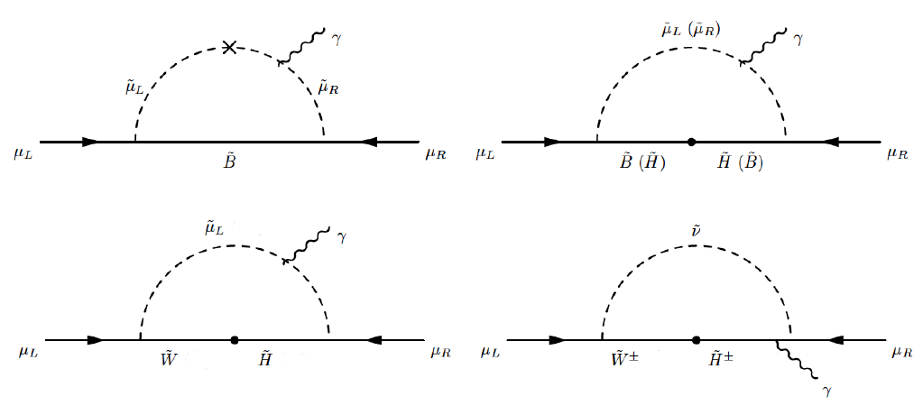
Figure 1: The leading contributions to muon $g-2$ involving neutralino and chargino loops. The cross in the top-left diagram denotes the chirality flip between the left- and right-handed smuons, while the dots in the other diagrams represent the mixing between different neutralino species. In the top-right diagram, there is another loop which is formed by the particles given in the parentheses.

The SUSY contributions to muon $g-2$ can arise at one-loop from the electroweak gauginos, Higgsinos and sleptons through the diagrams shown in Fig. 1 Martin:2001st ; Giudice:2012pf ; Moroi:1995yh , and these contributions potentially fill the gap between the latest measurements Muong-2:2023cdq and the muon $g-2$ predctions SM Aoyama:2020ynm . However, the current experimental constraints, especially from the Higgs boson mass, can exclude the required relatively large contributions in the simplest SUSY models such as CMSSM. In addition, when leptons and sleptons mass matrices are not aligned in the same superfield basis, Lepton Flavor Violating (LFV) processes can occur through very similar topologies as shown in Fig. 2. In this section, we consider the muon $g-2$ and LFV processes and emphasize the interplay between them.

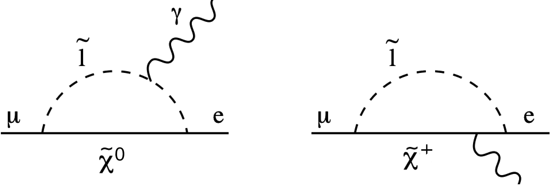
Figure 2: One-loop diagrams for the decay $\mu\rightarrow e\gamma$: $\tilde{l}$ represents a charged slepton (left) or sneutrino (right), and $\tilde{\chi}^{0}$, $\tilde{\chi}^{+}$ represent neutralinos and charginos respectively.

2.1 SUSY contribution to muon g-2

The supersymmetric contributions at the leading one-loop level are shown in Fig. 1. The dominant contributions calculated by the mass insertion Moroi:1995yh ; Stockinger:2006zn ; Cho:2011rk ; Fargnoli:2013zia can be summarized as

$$\Delta a_{\mu}^{SUSY}\simeq(\Delta a_{\mu}^{\tilde{B}\tilde{\mu}_{L}\tilde{\mu}_{R}}+\Delta a_{\mu}^{(\tilde{B}-\tilde{H})\tilde{\mu}_{L}}+\Delta a_{\mu}^{(\tilde{H}-\tilde{B})\tilde{\mu}_{R}}+\Delta a_{\mu}^{(\tilde{H}-\tilde{W})\tilde{\mu}_{L}}+\Delta a_{\mu}^{(\tilde{W}-\tilde{H})\tilde{\nu}_{\mu}}),$$ (1)

where the contribution from each diagram can be expressed as Cho:2011rk :

$$\Delta a_{\mu}^{\tilde{B}\tilde{\mu}_{L}\tilde{\mu}_{R}}\;\;\; = \phantom{-}\frac{g_{Y}^{2}}{8\pi^{2}}\frac{m^{2}_{\mu}\mu\tan\beta}{M_{1}^{3}}\ F_{b}\left(\frac{m^{2}_{\tilde{\mu}_{L}}}{M_{1}^{2}},\frac{m^{2}_{\tilde{\mu}_{R}}}{M_{1}^{2}}\right),$$ (2a)

$$\Delta a_{\mu}^{(\tilde{H}-\tilde{B})\tilde{\mu}_{R}} = -\frac{g_{Y}^{2}}{8\pi^{2}}\frac{m^{2}_{\mu}M_{1}\mu\tan\beta}{m^{4}_{\tilde{\mu}_{R}}}\ F_{b}\left(\frac{M_{1}^{2}}{m^{2}_{\tilde{\mu}_{R}}},\frac{\mu^{2}}{m^{2}_{\tilde{\mu}_{R}}}\right),$$ (2b)

$$\Delta a_{\mu}^{(\tilde{B}-\tilde{H})\tilde{\mu}_{L}} = \phantom{-}\frac{g_{Y}^{2}}{16\pi^{2}}\frac{m^{2}_{\mu}M_{1}\mu\tan\beta}{m^{4}_{\tilde{\mu}_{L}}}\ F_{b}\left(\frac{M_{1}^{2}}{m^{2}_{\tilde{\mu}_{L}}},\frac{\mu^{2}}{m^{2}_{\tilde{\mu}_{L}}}\right),$$ (2c)

$$\Delta a_{\mu}^{(\tilde{W}-\tilde{H})\tilde{\nu}_{\mu}} = -\frac{g^{2}}{16\pi^{2}}\frac{m^{2}_{\mu}M_{2}\mu\tan\beta}{m^{4}_{\tilde{\mu}_{L}}}\ F_{b}\left(\frac{M_{2}^{2}}{m^{2}_{\tilde{\mu}_{L}}},\frac{\mu^{2}}{m^{2}_{\tilde{\mu}_{L}}}\right),$$ (2d)

$$\Delta a_{\mu}^{(\tilde{W}-\tilde{H})\tilde{\nu}_{\mu}} = \phantom{-}\frac{g^{2}}{8\pi^{2}}\frac{m^{2}_{\mu}M_{2}\mu\tan\beta}{m^{4}_{\tilde{\nu}}}\ F_{a}\left(\frac{M_{2}^{2}}{m^{2}_{\tilde{\nu}}},\frac{\mu^{2}}{m^{2}_{\tilde{\nu}}}\right).$$ (2e)

whith,

$$F_{a}(x,y) = -\dfrac{1}{2(x-y)}\left[\dfrac{(x-1)(x-3)+2\ln(x)}{(x-1)^{3}}-\dfrac{(y-1)(y-3)+2\ln(y)}{(y-1)^{3}}\right]~{},$$ (3a)

$$F_{b}(x,y) = -\dfrac{1}{2(x-y)}\left[\dfrac{(x-1)(x+1)+2x\ln(x)}{(x-1)^{3}}-\dfrac{(y-1)(y+1)+2y\ln(y)}{(y-1)^{3}}\right].$$ (3b)

In the framework of the $4-2-2$ symmetry presented in Ref. Gomez:2022qrb , we find models that can provide simultaneous explanations for the measured muon $g-2$ and the desired DM candidate consistent with the Planck measurements Planck:2018nkj . Typically, the main SUSY contributions to muon $g-2$ in our models come from the processes represented with the top-left and bottom-right diagrams of Fig. 1, corresponding to Eqs.(2a) and (2e), respectively. The dominance of one or the other diagram can be associated with different features of the model, such as the nature of LSP and its mass difference with the other SUSY particles that coannihilate with it in order to explain the observed DM abundance. All contributions are proportional to $\mu\tan\beta$, however, the value of this term is limited by RGE-induced electroweak symmetry breaking (EWSB) and the vacuum stability of the MSSM scalar potential Carena:2012mw .

SUSY Scale	GUT Scale
$m_{\tilde{\mu}_{L}},m_{\tilde{\nu}}$	$m_{L}$
$m_{\tilde{\mu}_{R}}$	$m_{R}$
$M_{\tilde{B}}$	$M_{1}$
$M_{\tilde{W}}$	$M_{2L}$
$\mu$	$m_{H_{u}},m_{H_{d}}$
$A_{\mu}$	$A_{0}$
$\tan\beta$	$\tan\beta$

Table 1: The fundamental parameters determining the supersymmetric contributions to muon $g-2$ at the low scale (left) and the GUT scale (right).

2.2 LFV decays in SUSY 4-2-2.

We will work within the $4-2-2$ framework presented in Ref. Gomez:2022qrb . The relevant SUSY parameters at the GUT scale are listed in Table 1. As previously shown, in this framework the muon $g-2$ solutions favor heavy gluinos, while the LSP can still be a good DM candidate with masses lighter than about 500 GeV. The heavy gluinos enhance the squark masses through RGEs, thus leading to a significant splitting between the squarks and slepton masses. This can easily be seen by using the approximate RGE solutions provided in Refs. Ibanez:1984vq ; Martin:1997ns that show an approximate relation between the GUT scale parameters and the low energy mass terms.

$$m_{\tilde{Q}_{i}}^{2}\!\!\! = \!\!\!m_{L}^{2}+K_{3}+K_{2}+{\frac{1}{36}1}K_{1},$$

$$m_{\tilde{U}_{i}}^{2}\!\!\! = \!\!\!m_{R}^{2}+K_{3}\qquad\>\>\>+{\frac{4}{9}}K_{1},$$

$$m_{\tilde{D}_{i}}^{2}\!\!\! = \!\!\!m_{R}^{2}+K_{3}\qquad\>\>\>+{\frac{1}{9}}K_{1},$$

$$m_{\tilde{e}_{Li}}^{2}\!\!\! = \!\!\!m_{L}^{2}\qquad\>\>\>+K_{2}+{\frac{1}{4}}K_{1},$$

$$m_{\tilde{e}_{Ri}}^{2}\!\!\! = \!\!\!m_{R}^{2}\qquad\qquad\>\>\>\>\>\>\,+\,K_{1}.$$ (4)

The quantities $K_{3}$, $K_{2}$ and $K_{1}$ from the RG running proportional to the gaugino masses. Explicitly, they are found at one loop order by solving the RGEs, as given for example in Ref. Martin:1997ns :

$$K_{i}(Q)=\begin{Bmatrix}{3/5}&\\ {3/4}&\\ {4/3}\end{Bmatrix}\times\frac{1}{2\pi^{2}}\int^{{\rm ln}M_{GUT}}_{{\rm ln}Q}dt\>\,g^{2}_{a}(t)\,|M_{i}(t)|^{2}\qquad\>\>\>(i=1,2,3),$$ (5)

where the running parameters $g_{i}(Q)$ and $M_{i}(Q)$ obey the RGEs given in Ref. Martin:1997ns .With the values of $Q=M_{SUSY}=\sqrt{m_{\tilde{t}_{1}}m_{\tilde{t}_{2}}}$ that we find in our models, the ranges of these amounts are:

$$K_{1}\approx 0.15\times(M_{1}^{GUT})^{2},\quad K_{2}\approx(0.3-0.5)\times(M_{2}^{GUT})^{2},\quad K_{3}\approx(4.3-6.7)\times(M_{3}^{GUT})^{2}.$$ (6)

Although this approximation is only valid for cases where first and second generation Yukawa couplings can be neglected still it provides a good picture of the mass splitting among sqarks and sfermions. Furthermore, these equations can show how a possible flavor dependence of the scalar soft terms can be transmitted to the low energy observables. For instance, we observe that the sfermion masses at the TeV scale have a flavor independent component arising from gauginos in addition to the contribution from the soft scalar masses, that can be flavor dependent. This may induce misalignments between the fermion Yukawa and the sfermion mass matrices. Typically, in SUSY models the flavor mixture of the soft terms results in fermionic flavor violating decays, very constrained by the strong bounds on flavor changing neutral currents (FCNC). However, in the $4-2-2$ framework we find that the large gluino masses suitable for explaining muon $g-2$, and the lower masses for $M_{1},M_{2}$ that can explain DM, can suppress such processes on the quarks while being less restrictive on the leptonic sector. For instance, according to Eqs. 4 only diagonal mass terms grow with gaugino masses, thus the flavour mixing in the squark mass matrices are washed out by the large gluino contribution to the diagonal ones, such that their contribution to processes like $b\rightarrow s\gamma$ Olive:2008vv is not significant. On the other hand, the moderate values we find for the lighter gauginos do not suppress the effect of the slepton mass mixing terms, leading to the prediction of charged lepton violating (cLFV) decays on the range of the experimental searches Gomez:2010ga .

Flavor dependent scalar soft terms can be induced below the GUT scale through the RGEs when a mechanism like the see-saw is present in the theory to explain neutrino masses. Also, the flavor dependence can be generated above the GUT scale if the GUT symmetry is combined with additional ones to explain the favour hierarchy in the Yukawa interactions.

In the current work, we use gauge group $4-2-2$ without imposing Left-Right (LR) symmetry (for a detailed description see Gomez:2020gav ; Gomez:2022qrb and references therein). Such symmetries can emerge from $SO(10)$ breaking by the Higgs fields in $210_{H}$ representation Babu:2016bmy . Assuming type I see-saw, cLFV will be induced below the GUT scale. The running of the slepton masses from $M_{GUT}$ to $M_{R}$ is affected by the Dirac neutrino Yukawa coupling matrix $Y_{\nu}$, that can be of the same order as the fermion Yukawa couplings. Therefore, flavor-changing terms for the slepton masses are introduced since $Y_{\nu}$ cannot be diagonalised in the same basis as the charged lepton Yukawa matrix $Y_{l}$. For instance, in a basis where $Y_{l}$ is diagonal at the leading-log approximation Hisano:1995cp , the non-diagonal terms of the lepton mass matrix take the following form at scale $M_{R}$:

$$(m_{\tilde{L}}^{2})_{ij} \sim \frac{1}{16\pi^{2}}(6m^{2}_{0}+2A^{2}_{0})\left({Y_{\nu}}^{\dagger}Y_{\nu}\right)_{ij}\log\left(\frac{M_{\rm GUT}}{M_{R}}\right)\,,$$

$$(m_{\tilde{e}}^{2})_{ij} \sim 0\,,$$

$$(A_{l})_{ij} \sim \frac{3}{8\pi^{2}}{A_{0}Y_{l}}_{i}\left({Y_{\nu}}^{\dagger}Y_{\nu}\right)_{ij}\log\left(\frac{M_{\rm GUT}}{M_{R}}\right)\,.$$ (7)

In addition, to explain fermion flavour it is possible to combine family symmetries with the GUT group to build predictive Yukawa textures Ibanez:1994ig ; Lola:1999un ; Ellis:1998rj ; Kane:2005va ; King:2000ge ; Dent:2004dn . In some of these frameworks, the appropriate hierarchy among couplings can be reproduced with a single parameter obtained through the Froggatt-Nielsen mechanism Froggatt:1978nt . Moreover, in models with soft SUSY breaking terms derived from supergravity, flavor dependent scalar soft terms can be induced above the GUT scale when the unifying symmetry is combined with additional groups under which the fermion families carry different charges. Consider, for instance, higher order operators at some high scale $M$:

$$\Phi_{i}\Phi_{J}^{c}h\;\frac{\theta^{(q_{i}-q_{j}+q_{h})}}{M},$$ (8)

where $\Phi_{i}$ and $\Phi_{j}^{c}$ ($i,j=1,2,3$) denote quark/lepton superfields, h is a Higgs superfield, and $\theta$ represents the flavon field, which develops a non-zero vacuum expectation value (VEV) such that a small expansion parameter is induced, $\epsilon=\dfrac{\langle\theta\rangle}{M}$, where $\langle\theta\rangle$ is the flavon VEV. If the flavor symmetry is chosen to be an abelian $U(1)$ group, the hierarchy among the flavors can arise from non-universal charges of the families under this group. Even if flavor-independent soft terms are assumed above the GUT scale, the soft terms generated at $M_{{\rm GUT}}$ are flavor-dependent. Their flavor structure depends on the family charges, normalization of Kähler potential, and the rotation of the Yukawa matrices King:2004tx ; Das:2016czs . Therefore, in a field basis where the fermion mass matrices are diagonal, the corresponding sfermion matrix takes the form:

$$m_{f}^{2}=\begin{pmatrix}1&\epsilon^{q^{12}}&\epsilon^{q^{13}}\\ \epsilon^{q^{12}}&1&\epsilon^{q^{23}}\\ \epsilon^{q^{12}}&\epsilon^{q^{23}}&1\\ \end{pmatrix}\times m_{f^{0}}^{2},$$ (9)

where $q^{i,j}$ are combinations of charges of the generations $i,j=1,2,3$, and $m_{f^{0}}$ is a common soft SUSY breaking mass.

Due to the lack of LR symmetry, the sfermions mass matrices are independently induced for the left- and right-handed fields, and their flavor-dependent forms can be written as follows:

$$m_{f}^{2}=\begin{pmatrix}1&\epsilon^{q_{L}^{12}}&\epsilon^{q_{L}^{13}}\\ \epsilon^{q_{L}^{12}}&1&\epsilon^{q_{L}^{23}}\\ \epsilon^{q_{L}^{12}}&\epsilon^{q_{L}^{23}}&1\\ \end{pmatrix}\times m_{L}^{2},\hskip 14.22636ptm_{f^{c}}^{2}=\begin{pmatrix}1&\epsilon^{q_{R}^{12}}&\epsilon^{q_{R}^{13}}\\ \epsilon^{q_{R}^{12}}&1&\epsilon^{q_{R}^{23}}\\ \epsilon^{q_{R}^{12}}&\epsilon^{q_{R}^{23}}&1\\ \end{pmatrix}\times m_{R}^{2}~{},$$ (10)

where $m_{L}$ and $m_{R}$ are the soft sypersymmetry breaking (SSB) masses for the left- and right-handed sfermions. These matrices are induced both in the squark the slepton sectors. However, because of the heavy squarks driven by the heavy gluinos through RGEs, the flavor mixing in these matrices is suppressed and their flavor mixing in essentially coincides with the CKM matrix. On the other hand, even though the charged lepton Yukawa matrix remains diagonal in this basis, the non-diagonal form of the slepton mass-squared matrix can induce the cLFV processes such as $l_{i}\rightarrow l_{j}\gamma$ at the loop level, as shown diagrammatically in Fig. 2.

In summary we classify the LFV scenarios according to the scale where mixing of the soft terms is introduced:

• LFV below the GUT scale. In this case the soft terms are taken to be universal at $M_{GUT}$, and LFV is induced through a type I see-saw mechanism We use the simplified scenario presented in Ref. Ellis:2020jfc , where a simple but representative case was obtained by considering a common RH neutrino mass $M_{R}$ is assumed for the three species. In this case, using Casas:2001sr , we find for the see-saw parameters that enter eq. (7):

  $$Y_{\nu}^{\dagger}Y_{\nu}=\frac{2}{v_{u}^{2}}M_{R}Um_{\nu}^{\delta}U^{\dagger}~{}.$$ (11)

  Using a basis in which the charged lepton Yukawa matrix is diagonal, $U$ can be identified with the Pontecorvo-Maki-Nakagawa-Sakata (PMNS) matrix, while $m_{\nu}^{\delta}$ is the diagonal neutrino mass matrix. $U$ is set to the central values of the experimental data ParticleDataGroup:2022pth , while the values $m_{\nu}^{\delta}=Diag(1.1\cdot 10^{-3},8\cdot 10^{-3},5\cdot 10^{-2})$ eV are compatible with the observed neutrino oscillations, assuming direct mass hierarchy. With the assumption of common masses for the heavy Majorana neutrinos, the LFV effects are independent of textures for the matrices $M_{R}$ and $Y_{\nu}$, which in some cases can lead to some cancellations in the LFV branching ratios Cannoni:2013gq . However, these ratios are strongly dependent on $M_{R}$. Here, we assume $M_{R}=2.5\times 10^{12}$ GeV and, with this choice, we obtain values for BR($\mu\rightarrow e\gamma$) of the order of the current or projected experimental bounds.

• Family symmetries with flavor dependent soft terms at $M_{GUT}$. In this case, we assume flavor mixing among the charged leptons from Eqs. (10). We consider two separate cases, namely weak flavor mixing ($\epsilon=0.05$), and strong flavor mixing ($\epsilon=0.2$). In our computations we select $q_{L}^{12}=q_{L}^{13}=3$, $q_{L}^{23}=2$ and $q_{R}^{12}=4$, $q_{R}^{13}=q_{L}^{23}=2$. These values, together with $\epsilon$, provide predictions for BR($\mu\rightarrow e\gamma$) that are compatible with both the experimental data and the results we obtain from the see-saw model. We should remark that our choice of charges and values for $\epsilon$ is not aimed at a full explanation of the hierarchy of the Yukawa coupling matrices that may require, in addition to the family symmetries, a complex Higgs potential that splits quarks and leptons from the L and R multiplets in $4-2-2$ King:2000ge ; Dent:2004dn . Also, we neglect in this case the possible see-saw effects which can be consistent with the assumption of right-handed neutrinos masses $M_{N}\lesssim\mathcal{O}(10^{10})$  GeV, accompanied by very small Dirac Yukawa couplings between the Higgs boson and neutrinos ($Y_{\nu}\lesssim 10^{-7}$) Coriano:2014wxa ; Khalil:2010zza ; Abbas:2007ag ; Un:2016hji , leading to tiny contributions to LFV processes.

3 Fundamental Parameters and Experimental Constraints

We perform random scans in the fundamental parameter space of 4-2-2 with broken LR symmetry by using SPheno-4.0.4 Porod:2003um ; Porod:2011nf , which is implemented by SARAH-4.14.4 Staub:2008uz . The values for the input parameters at the GUT level used in the 4-2-2 model described above are:

$$\begin{array}[]{lll}0\leq&m_{L}&\leq 5~{}{\rm TeV}\\ 0\leq&M_{2L}&\leq 5~{}{\rm TeV}\\ -3\leq&M_{3}&\leq 5~{}{\rm TeV}\\ -3\leq&A_{0}/m_{L}&\leq 3\\ 1.2\leq&\tan\beta&\leq 60\\ 0\leq&{\rm x}_{{\rm LR}}&\leq 3\\ -3\leq&{\rm y}_{{\rm LR}}&\leq 3\\ 0\leq&{\rm x}_{{\rm d}}&\leq 3\\ -1\leq&{\rm x}_{{\rm u}}&\leq 2~{}.\\ \end{array}$$ (12)

Here, $m_{L}$ is the SSB mass term for the left-handed sfermions and $M_{2L}$, $M_{3}$ stand for the SSB masses of $SU(2)_{L}$ and $SU(3)_{c}$ gauginos, respectively. The LR symmetry breaking in the sfermions and gauginos is controlled by ${\rm x}_{{\rm LR}}$ and ${\rm y}_{{\rm LR}}$, namely $m_{R}={\rm x}_{{\rm LR}}m_{L}$ and $M_{2R}=y_{LR}M_{2L}$, where $M_{2R}$ denotes the SSB mass of $SU(2)_{R}$ gaugino. Similarly, $x_{d}$ and $x_{u}$ parametrize the non-universality in the SSB masses at $M_{{\rm GUT}}$ of the MSSM Higgs fields, $m_{H_{d}}^{2}=x_{d}m_{L}^{2}$ and $m_{H_{u}}^{2}=x_{u}m_{L}^{2}$. In addition, we vary the universal trilinear scalar interaction term $A_{0}$ by requiring that the magnitude of its ratio to $m_{L}$ is not greater than 3, to avoid the color/charge breaking minima of the scalar potential Ellwanger:1999bv ; Camargo-Molina:2013qva ; Camargo-Molina:2013sta . In scanning the parameter space we use the Metropolis-Hastings algorithm Belanger:2009ti ; Baer:2008jn , and generate the solutions by following flat priors Trotta:2008bp .

As indicated in the previous section, we introduce LFV in three different scenarios. One is simplified seesaw Type 1 where the flavor mixing among left sleptons is induced by RGEs. The other two scenarios mix the slepton flavors at scales above $M_{{\rm GUT}}$. The texture is chosen so that, for $\epsilon=0.05$, it provides values for BR($\mu\rightarrow e\gamma$) comparable to the seesaw case, while for $\epsilon=0.2$ it may strongly restrict the GUT values of the soft masses, allowing only models comparable with ”no-scale” SUSY Lahanas:1986uc ; Ellis:2013nka ; Li:2016bww ; Ford:2019kzv ; Li:2021cte . We impose the the bounds ParticleDataGroup:2022pth :

$${\rm BR}(\mu\rightarrow e\gamma) < 4.2\times 10^{-13}~{},$$ (13)

$${\rm BR}(\tau\rightarrow e\gamma) < 4.3\times 10^{-8}~{},$$ (14)

$${\rm BR}(\tau\rightarrow\mu\gamma) < 3.2\times 10^{-8}.$$ (15)

In our search, we keep the points that satisfy the constraints:

$$\begin{array}[]{c}m_{h}=123-127~{}{\rm GeV}~{},\\ m_{\tilde{g}}\geq 2.1~{}{\rm TeV}~{}(800~{}{\rm GeV}~{}{\rm if~{}it~{}is~{}NLSP})~{},\\ 0.8\times 10^{-9}\leq{\rm BR}(B_{s}\rightarrow\mu^{+}\mu^{-})\leq 6.2\times 10^{-9}\;(2\sigma)~{},\\ 2.99\times 10^{-4}\leq{\rm BR}(B\rightarrow X_{s}\gamma)\leq 3.87\times 10^{-4}\;(2\sigma)~{},\\ 0.114\leq\Omega_{{\rm CDM}}h^{2}\leq 0.126~{}.\end{array}$$ (16)

In addition to requiring the solutions to be consistent with these constraints, we also select those which predict muon $g-2$ within the $2\sigma$ band of its experimentally measured values and also include the interplay between the cLFV processes and muon $g-2$ contributions. Finally, we only accept solutions which are compatible with the LSP neutralino relic density either consistent or lower than the Planck measurements Planck:2015fie . The DM constraints together with the muon $g-2$ condition imposes a severe restriction on the possible DM scenarios, that are limited to the following cases:

• 

  

  

  Figure 3: Values of $\Omega h^{2}$ vs $m_{\chi}$ for models satisfying the Planck upper bound on DM and the muon $g-2$ within $2\sigma$ in correlation with $m_{\chi}$. All the models predict charged lepton violating decays inside the experimental bounds. Different symbols and color codes are assigned to each class of model: blue crosses for annihilations, orange pluses for $\tilde{\tau}-\chi$ coannihilations, red crosses for $\tilde{\nu}-\tilde{\tau}-\chi$ coannihilations, black pluses for $\chi^{\pm}-\chi$ coannihilations. The left panel corresponds to the see-saw case, while the two others correspond to scenarios with U(1) family symmetries. The centre one uses $\epsilon=0.05$ as expansion parameter while the right one uses $\epsilon=0.2$.

• $\chi$-annihilations. This scenario implies low mass values for the SUSY partners involved in the muon $g-2$ computations. The LSP is mostly a Bino with annihilation cross section large enough to explain DM. The lightest sleptons are mostly right-handed.

• $\chi-\tilde{\tau}$-coannihilations. This scenario implies a wider spectrum than the previous one. The LSP is also a Bino but, in this case, models explaining the muon $g-2$ require low values for mostly right sleptons, that also decrease the DM abundance to Planck levels.

• $\chi-\tilde{\tau}-\tilde{\nu}$-coannihilations. This scenario is enabled by $L/R$-symmetry breaking, which allows for the possibility of left sleptons lighter than the right ones. In this scenario, the light $\tilde{\nu}$ becomes the NLSP that enters the coannihilation scenario and also increases the contribution to muon $g-2$.

• $\chi-\tilde{\chi}^{\pm}$-coannihilations. This scenario is allowed because of the gaugino mass relations introduced by the 4-2-2 symmetry. In this case, the LSP is a Wino while the lightest chargino is the NLSP. Values of the chargino masses are close to neutralinos and sleptons allow for relatively large values for muon $g-2$. However, many of the models predict relic densities below the Planck bounds. Therefore, the models, while cosmological viable, cannot resolve the DM problem.

Fig. 3 displays the values of $\Omega_{\chi}h^{2}$ vs the LSP mass for the three different scenarios under consideration. Each of the coannihilation scenarios listed above is shown with different colors and symbols as given in legends. We observe that a particle coannihilates with the LSP when its mass is up to 30% larger than the LSP. In many cases, there are other particles in this range of mass in addition to the NLSP. We find models with $m_{\chi}$ below 100 GeV that satisfy the Planck bounds without coannihilations. Such solutions represent the annihilation of LSP into the SM particles.

Different DM areas can be associated with the dominant contributions to the muon $g-2$. In models with Bino-like LSP, the dominant contribution (eq. 2a) arises from the upper left diagram of Fig. 1, while the lower right diagram is the dominant one in scenarios with Wino-like LSP (eq. 2e). The contribution from this diagram is also enhanced by a light $\tilde{\nu}_{\mu}$. The LR asymmetry of the soft terms, together with $M_{2}>M_{1}$, allows the left sleptons to become lighter than the right ones. This selection of soft terms favors both SUSY contributions to muon $g-2$ and a relic density of LSP below the upper Planck bound. However, the small mass differences between the lightest SUSY particles produce significant changes in $\Omega h^{2}$. Indeed, models in Fig. 7 change from Bino to Wino LSP as $M_{1}$ increases. In regions with $M_{1}\sim M_{2}$, we obtain a zone between models with $\tilde{\tau}$ (orange points) or chargino NLSP (black crosses), where $\tilde{\nu}_{\tau}$ becomes the NLSP (red points). The nature of the LSP also plays an important role in DM implications. In the solutions with Wino-like LSP, we obtain a zone between models with $\tilde{\tau}$ (orange points) or chargino NLSP (black crosses), where $\tilde{\nu}_{\tau}$ becomes the NLSP (red points). Such solutions can be associated with $M_{1}\sim M_{2}$.

4 Analysis and Results

4.1 Slepton masses and LFV

As previously mentioned, flavor violation is induced through the flavor-dependent mass matrices, but the large values of $M_{3}$ (see Fig. 8) drives the diagonal entries to be quite large in the squark mass-squared matrices. Thus, the flavor violating entries do not have a strong impact in the quark sector. On the other hand, the desired muon $g-2$ values require moderate masses for the sleptons and electroweak gauginos, which implies $M_{1},M_{2}\ll M_{3}$. In this context, the GUT scale mass-squared matrices with the flavor violating entries can have considerable effects in the slepton mass spectrum, especially in the solutions leading to slepton-neutralino coannihilation processes.

Figure 4: BR($\mu\rightarrow e\gamma$) vs $m_{\chi}$ for the three models discussed in the text. Order of the panels, symbols and color codes are as in Fig. 3. In addition the points with relic density inside the Plank bounds are colored in green.

Figure 5: GUT scale values of $m_{L}$ vesus $m_{R}$. Order of panels, symbols and colors are as in Fig. 3. We mark in green the points with relic density inside Planck bounds all the points satisfy the BR($\mu\rightarrow e\gamma$) constraint.

The predictions for BR($\mu\rightarrow e\gamma$) vs $m_{\chi}$ are displayed in Fig. 4 for the three mixing scenarios under consideration. Confronting the results for $\mu\rightarrow e\gamma$ with the scales of $m_{L}$ and $m_{R}$ shown in Fig. 5, we can summarize our findings as follows:

• In the seesaw scenario the constraint from $\mu\rightarrow e\gamma$ is very restrictive for the solutions with $m_{L}\gtrsim 100$ GeV, while it is less so for larger $m_{R}$ values. In contrast to the other scenarios, where the LFV terms are induced at $M_{{\rm GUT}}$, solutions with low values of $m_{L/R}$ are not allowed in the seesaw scenario. The LEP limit on masses of the charged particles leads to a lower bound on $m_{L}$ and $m_{R}$ of about 20 GeV due to the light staus.

• In the scenario with $\epsilon=0.05$ (middle planes in Figs. 4 and 5), the $\mu\rightarrow e\gamma$ constraint restricts the scales for the sfermion masses as $m_{L}\lesssim 90$ GeV and $m_{R}\lesssim 50$ GeV, while beyond these limits the LFV processes become significant. In the region where the relic density is inside the Planck bound, the prediction for ${\rm BR}(\mu\rightarrow e\gamma)$ is one or two orders of magnitude lower than the experimental limit. The LSP in these regions is mostly Bino-like, and the desired DM relic density can be realized through stau-nuetralino coannihilation and annihilations of LSP pairs, while models with chargino-neutralino coannihilations predict a relic DM density below the Planck bound.

• The third scenario with $\epsilon=0.2$ is obviously affected more by the LFV constraints (left panel of Fig. 2). Comparing with the left panel of Fig. 5, the only solutions consistent with the LFV constraints lie in the regions where $m_{L}\lesssim 15$ GeV and $m_{R}\lesssim 40$ GeV. The LSP neutralino relic density is reduced to the required ranges through the chargino-neutralino coannihilations in these solutions. Even though the LFV constraints are weaker for large values of $m_{R}$, it is also possible to realize some solutions consistent with the LFV constraints and even DM observations in the regions where $m_{L}<m_{R}\sim 100$ GeV.

In sum, the $\mu\rightarrow e\gamma$ constraint seems more restrictive in models where flavor mixing is introduced above $M_{{\rm GUT}}$. The seesaw mechanism induces LFV only in the left-handed sleptons while the scenarios with non-zero $\epsilon$ generate flavor mixing in both the left- and right-handed sfermions, thus enhancing the rates for the flavor violating processes. This can be potentially dangerous for decays such as $b\rightarrow s\gamma$ Olive:2008vv . Even though this enhancement can be suppressed by heavy masses as in the case of squarks, the condition of muon $g-2$ solution within $2\sigma$ does not allow heavy masses for sleptons and electroweak gauginos. In the mass scales favored by the muon $g-2$ solution, the cLFV rates are enhanced by the masses of sleptons, and as a result, we observe a stronger impact on $m_{L}$ and $m_{R}$ from cLFV constraints in these two scenarios.

Figure 6: BR($\mu\rightarrow e\gamma$) vs. BR($\tau\rightarrow\mu\gamma$), the panles, color codes and symbols represent the same models as in the previous Fig.4.

Another important observation is the correlation of the BR($\mu\rightarrow e\gamma$) with other cLFV decays, such as $\tau\rightarrow\mu\gamma$. Generic see-saw models predict more or less the same rate for these decays, while the experimental bounds differ by several orders of magnitude. On the other hand, in general, the prediction for flavor mixing related to the family symmetry can allow a different hierarchy for the LFV $\tau$ and $\mu$ decays. In Fig. 6 we display BR($\mu\rightarrow e\gamma$) vs BR($\tau\rightarrow\mu\gamma$), and observe that scenarios with family symmetries can predict branching ratios for these decays in ranges closer to the experimental values. In addition to fitting the models with the current cLFV constraints, the solutions will be potentially tested soon by the improvements and upgrades in MEG II MEGII:2018kmf ; MEGII:2023ltw ; MEGII:2023fog , Mu2e Hedges:2022tnh , COMET COMET:2018auw and DeeMe Teshima:2019orf . decays

Figure 7: GUT values of $M_{2}$ vs $M_{1}$. Order of panels, symbols and colors are as in Figs. 3 and 5.

Figure 8: GUT values of $M_{3}$ vs $M_{1}$. Order of panels, symbols and colors are as in Figs. 3 and 5.

4.2 Muon g-2 and SUSY Masses

As discussed in the previous sections, the muon $g-2$ condition imposed within $2\sigma$ band of its experimental measurements shapes the mass spectrum for the sleptons and electroweak gauginos. Fig. 7 shows the allowed scales for $M_{2}$ and $M_{1}$ for each scenario. As a result of the allowed cLFV processes, the parameter space is squeezed from left to right in these panels. These two soft masses play a crucial role in determining the LSP composition. As seen in all the planes, the chargino-neutralino coannihilations (black plus) mostly happen for $M_{2}<M_{1}$, where the LSP is composed mostly of Wino. Even though these solutions are not excluded by the cosmological observations, they yield a very low relic density for LSP neutralino and therefore cannot account for the observed DM abundance. If the Bino takes part in the LSP composition, the stau (and stau-sneutrino)-neutralino coannihilations can also be identified. For very light ($\lesssim 200$ GeV) $M_{1}$, or if $M_{2}$ is relatively heavy ($\gtrsim 700$ GeV), the NLSP mass is beyond the range for suitable coannihilation scenarios and the LSP relic density is reduced through pair annihilations.

We have also displayed the scales for $M_{3}$ in Fig. 8 which summarizes the statements of suppressed flavor mixings in the quark sector due to the heavy gluinos in the regions favored by the muon $g-2$ condition. Recall that despite the light scales for $m_{L}$ and $m_{R}$, the dominant enhancement in the squark masses arises mostly from $M_{3}$ through RGEs. The large squark masses due to the heavy gluinos are also helpful in realizing the desired SM-like Higgs boson mass. In the MSSM framework the loop correction to the SM-like Higgs boson mass is given by Carena:2012mw

Figure 9: $tan\beta$ vs $m_{\chi}$. Order of panels, symbols and colors are as in Figs. 3 and 5.

$$\Delta m_{h}^{2}\simeq\dfrac{m_{t}^{4}}{16\pi^{2}v^{2}\sin^{2}\beta}\dfrac{\mu A_{t}}{M^{2}_{{\rm SUSY}}}\left[\dfrac{A_{t}^{2}}{M^{2}_{{\rm SUSY}}}-6\right]+$$

$$\hskip 39.83368pt\dfrac{y_{b}^{4}v^{2}}{16\pi^{2}}\sin^{2}\beta\dfrac{\mu^{3}A_{b}}{M^{4}_{{\rm SUSY}}}+\dfrac{y_{\tau}^{4}v^{2}}{48\pi^{2}}\sin^{2}\beta\dfrac{\mu^{3}A_{\tau}}{m_{\tilde{\tau}}^{4}}~{}~{},$$ (17)

where $M_{{\rm SUSY}}\equiv\sqrt{m_{\tilde{t}_{L}}m_{\tilde{t}_{R}}}$. The first line of Eq. 17 represents the contributions from the stops, and the contributions depicted in the second line come from the sbottom and stau, respectively. The contribution from stops is dominant in Eq. (17), whereas the contributions from the sbottom and stau can be important for moderate and large $\tan\beta$ values. However, large $\tan\beta$ values cannot simultaneously accommodate together with the muon $g-2$ condition due to the inconsistently light SM-like Higgs boson mass (for details, see Gomez:2022qrb ). Even though $\tan\beta$ can be as high as about 40 and 35 in the models displayed in the left and middle planes of Fig. 9, the Higgs boson mass bounds limit it to $\tan\beta\lesssim 17$ in the models with $\epsilon=0.2$, as shown in the right plane.

Figure 10: $\mu$ vs $M_{3}$. Order of panels, symbols and colors are as in Figs. 3 and 5.

A good prediction for Higgs boson mass favors maximal mixing of the stops Gomez:2022qrb , but it disfavors the SUSY contribution to muon $g-2$. However, it is possible to find some values of the $\mu$-term that allow compatible predictions for both observables. For instance, in Fig. 10 we show that some solutions can be realized for $1\lesssim\mu\lesssim 2$ TeV, while most of the soluions yield values from 2 Tev to 6 TeV. In addition, we observe, that imposing the DM bounds requires the values of $M_{3}$ and $\mu$ to be strongly correlated.

Figure 11: Spin-independent cross section in correlation with the LSP mass. Order of panels, symbols and colors are as in Figs. 3 and 5. The solid lines are bounds from XENONnT XENON:2023cxc (black) and LZ LZ:2022lsv (red), while dashed lines are the projected limits from XENON-nT XENON:2015gkh (black) and DARWIN DARWIN:2016hyl (blue).

The discussion of muon $g-2$ and SUSY mass spectra together with the DM implications should be supplemented with the possible DM detection scenarios in the direct detection experiments. In particular, the model prediction are within reach of the current sensitivities in underground experiments LZ:2022lsv ; XENON:2023cxc ; PandaX-4T:2021bab ; DEAP:2019yzn and the the projected limits from XENON-nT XENON:2015gkh and DARWIN DARWIN:2016hyl . However, the prediction for spin-dependent cross sections are lower than $10^{-7}pb$, and therefore below the current bounds from Amole_2019 . As seen from the panels of Fig. 11, there are models which satisfy the DM relic density consistent with the Planck measurements. The solutions lying between the solid and the dashed curves provide a potential test for these models via the direct detection experiments of DM, and the solutions lying close to the current LZ bound are expected to be tested soon. As shown in Fig. 11, most of the predictions consistent with the Planck DM bounds will be explored. Moreover, all of the models with $\epsilon=0.2$ will be tested.

4.3 LFV versus LHC spectroscopy

Figure 12: $m_{\tilde{\tau}}-m_{\chi}$ plots for models with BR($\mu\rightarrow e\gamma$) below the current bounds. Order of panels, symbols and colors are as in Figs. 3 and 5. The solid lines indicate the contours extracted by the LHC searches, while the cyan marks highlight models with BR($\mu\rightarrow e\gamma$) one order of magnitude below the current bound.

As seen in the previous section, the muon $g-2$ condition favors light neutralinos and charginos as well as smuons and its sneutrinos. This also implies the prediction of much lighter staus due to the larger L/R mixing in the third family. In this context, the interplay among muon $g-2$, DM and LFV constraints plays an essential role in selecting the parameter space and extracting experimental predictions. For instance, the light mass scales for stau, chargino and neutralino present an exciting opportunity for the current LHC experiments. Indeed, the light stau prediction can be tested in the collider analyses searching for the stau-pair production in which the staus decay into the LSP neutralino together with $\tau$. Even though all of the solutions presented in Fig. 12, fall below the bound from these analyses (red curve) due to the hadronic decays of $\tau$, the uncertainties are typically large since the desired precision in these analyses requires staus heavier than the LSP neutralino by 50 GeV or more CMS:2019hos ; ATLAS:2023djh . Thus, most of the solutions are still viable and there is considerable potential for future tests through upgrades in LHC precision. Moreover, the predictions for BR($\mu\rightarrow e\gamma$) in many of these models are less than an order of magnitude below the current bound, and therefore observable in the coming upgrade of MEG IIMEGII:2023ltw ; MEGII:2023fog .

Figure 13: $m_{\tilde{\chi}^{\pm}}-m_{\chi}$ plots for models with BR($\mu\rightarrow e\gamma$) below the current bounds. Order of panels, symbols and colors are as in Figs. 3 and 5. The solid curves indicate the contours extracted by the LHC searches, while the cyan marks highlight models with BR($\mu\rightarrow e\gamma$) one order of magnitude below the current bound.

A similar discussion holds for the charginos as displayed in Fig. 13 together with the bounds from the current LHC analyses. As seen here, all the models offer solutions which can be tested over a variety of different events such as those with leptons and/or b-quarks in the the final states. Furthermore, even the most restricted models with $\epsilon=0.2$ (right panel) provide some solutions that can be tested in $\bar{b}b$ and $l\bar{b}b$ events at the LHC. The compressed spectrum, on the other hand, has to wait for higher precision analyses to be tested. Therefore, the chargino-neutralino coannihilation solutions remain beyond the reach of the current collider experiments. However, the predictions for $\mu\rightarrow e\gamma$ in these models can be observable in the coming upgrade of MEG II MEGII:2023ltw ; MEGII:2023fog .

	Ps1	Ps2	Ps3	Ps4
$M_{1}$, $M_{2}$	495.4, 1373.4	727.3, 555.7	545.3, 542.6	649.5, 396.3
$M_{3}$	4970.7	3561.1	-970.9	2939.7
$m_{\widetilde{L}}$, $m_{\widetilde{R}}$	275.6, 247.0	263.7, 485.7	105.8, 246.9	369.5, 377.7
$A_{0}/m_{\widetilde{L}}$	0.5952	0.8346	1.463	-0.6759
$\tan\beta$	15.7	12.6	22.6	13.0
$\mu$, $m_{A}$	4994.1, 5000.7	3743.1, 3753.5	1103.4, 1034.3	3219.0, 3214.1
$m_{h}$, $m_{H,H^{\pm}}$	124.8, 5000	124.9, 3753	124.1, 1035	124.4, 3214
$m_{\tilde{\chi}_{1}^{0}}$,$m_{\tilde{\chi}_{2}^{0}}$	186.0, 1098.0	294.2, 409.7	242.6, 473.6	262.3, 283.6
$m_{\tilde{\chi}_{3}^{0}}$,$m_{\tilde{\chi}_{4}^{0}}$	5027.6, 5028.1	3768.8, 3769.3	1109.9, 1114.3	3239.3, 3239.8
$m_{\tilde{\chi}_{1}^{\pm}}$,$m_{\tilde{\chi}_{2}^{\pm}}$	1098.0, 5028.2	409.9, 3769.4	473.8, 1115.0	283.8, 3240.5
$m_{\tilde{g}}$	9773.2	7189.0	2141.8	6013.3
$m_{\tilde{l}_{1}}$,$m_{\tilde{l}_{2}}$	238.2, 359.5	297.2, 356.4	255.0, 319.0	296.4, 391.3
$m_{\tilde{l}_{3}}$, $m_{\tilde{l}_{4}}$	359.9, 814.2	356.7, 562.1	319.3, 387.3	391.8, 457.4
$m_{\tilde{l}_{5}}$, $m_{\tilde{l}_{6}}$	814.3, 818.4	562.2, 572.8	387.5, 415.0	457.8, 498.6
$m_{\tilde{\nu}_{1}}$,$m_{\tilde{\nu}_{2},\tilde{\nu}_{3}}$	794.4, 810	336.7, 348	371.9, 379	372.8, 384
$m_{\tilde{u}_{1}}$,$m_{\tilde{u}_{2}}$	8217.6, 8245.6	6092.9, 6109.4	1870.6, 1884.4	5121.9, 5126.7
$m_{\tilde{t}_{1}}$,$m_{\tilde{t}_{2}}$	7129.8, 7695.7	5297.7, 5695.0	1593.0, 1755.1	4412.6, 4776.5
$m_{\tilde{d}_{1}}$,$m_{\tilde{d}_{2}}$	8224.2, 8246.0	6093.4, 6112.2	1867.4, 1886.1	5122.6, 5129.1
$m_{\tilde{b}_{1}}$,$m_{\tilde{b}_{2}}$	7688.2, 8165.2	5684.2, 6082.7	1726.2, 1817.2	4763.4, 5101.3
$\Delta a_{\mu}\times 10^{10}$	14.8	15.4	17.5	16.3
$\Omega h^{2}$	0.12	0.12	0.11	0.09
$\sigma_{SI}(pb)$	$1.86\times 10^{-13}$	$6.82\times 10^{-13}$	$3.57\times 10^{-11}$	$1.01\times 10^{-12}$
$\sigma_{SD}(pb)$	$1.12\times 10^{-10}$	$3.52\times 10^{-10}$	$5.90\times 10^{-8}$	$6.90\times 10^{-10}$
$BR(\mu\rightarrow e\gamma)$	$8.7\cdot 10^{-16}$	$1.8\cdot 10^{-14}$	$6.5\cdot 10^{-14}$	$5.7\cdot 10^{-14}$
$BR(\tau\rightarrow\mu\gamma)$	$4.8\cdot 10^{-14}$	$3.1\cdot 10^{-13}$	$1.1\cdot 10^{-12}$	$1.2\cdot 10^{-142}$
$BR(\tau\rightarrow e\gamma)$	$6.6\cdot 10^{-16}$	$4.2\cdot 10^{-15}$	$1.5\cdot 10^{-14}$	$1.6\cdot 10^{-14}$

Table 2: Benchmark points for models type I see-saw, these models satisfy the same constraints of Eq. 16. All the points can explain the muon $g-2$ problem at $2-\sigma$ and predict neutralino relic density below the upper limit of the Planck measurements given in Eq. 16. We display in red the masses of the LSP and those which can coannihilate with LSP: P1 can explain relic density just with $\chi$ annihilations, and P2 corresponds to $\chi-\tilde{\tau}-\tilde{\nu}$, P3 to $\chi-\tilde{\tau}$, P4 to $\chi-\tilde{\chi}^{\pm}$.

Finally, we display two tables of benchmark points that are representative of our findings. The points listed in Table 2 belong to the seesaw models, and those in Table 3 represent the solutions realized in models with $\epsilon=0.05$ and $\epsilon=0.2$, as indicated in the header of Table 3. All of the benchmark points of seesaw scenario presented in Table 2 are compatible with the muon $g-2$ solutions within $2\sigma$, the Planck bound on the LSP neutralino relic density, and the constraint from $\mu\rightarrow e\gamma$. In addition, all these points, including P1, remain outside the contours of the current LHC bounds on the chargino and stau masses.

Similarly, the points in Table 3 depict several coannihilation scenarios realized in the other models as summarized in the caption. Although they are compatible with the muon $g-2$ requirement and the cLFV constraints, only P1 and P5 can be consistent with the Planck measurements. The remaining solutions usually lead to LSP neutralinos with a small relic density. The chargino-neutralino coannihilation solutions, in particular, yield a relatively small LSP relic density as shown with P4 and P6. The latter is one order of magnitude smaller than P4, since it simulatenously permits stau-neutralino coannihilations and chargino-neutralino coannihilations. However, these solutions can be consistently embedded in scenarios with multi-component the DM.

	P1, $\epsilon=0.05$	P2, $\epsilon=0.05$	P3, $\epsilon=0.05$	P4, $\epsilon=0.05$	P5, $\epsilon=0.2$	P6, $\epsilon=0.2$
$M_{1}$, $M_{2}$	375.8, 1318.6	694.7, 561.4	736.2, 662.1	1552.7, 240.8	146.6, 793.6	1281.4, 237.2
$M_{3}$	4065.4	2788.7	3038.3	3052.5	-1131.3	2172.6
$m_{\widetilde{L}}$, $m_{\widetilde{R}}$	227.8, 185.7	221.7, 207.4	221.3, 233.2	94.8, 172.4	32.7, 96.4	17.2, 19.4
$A_{0}/m_{\widetilde{L}}$	1.015	1.31	1.47	-0.82	0.013	-0.18
$\tan\beta$	13.4	7.5	8.9	13.5	9.7	10.6
$\mu$, $m_{A}$	4172.0, 4208.3	3021.4, 3140.3,	3243.3, 3325.8	3312.4, 3297.3	1240.7, 1342.5	2448.7, 2460.0
$m_{h}$, $m_{H,H^{\pm}}$	124.9, 4208.3	123.2, 3140.4	123.9, 3325.9	124.5, 3297.3	123.8, 1343.5	123.2, 2460.0
$m_{\tilde{\chi}_{1}^{0}}$,$m_{\tilde{\chi}_{2}^{0}}$	136.9, 1059.7	282.8, 424.6	300.8, 507.9	144.1, 652.5	72.0, 684.9	156.1, 535.9
$m_{\tilde{\chi}_{3}^{0}}$,$m_{\tilde{\chi}_{4}^{0}}$	4200.1, 4200.7	3041.6, 3042.6	3265.5, 3266.4	3334.2, 3334.7	1248.9, 1254.9	2463.9, 2464.8
$m_{\tilde{\chi}_{1}^{\pm}}$,$m_{\tilde{\chi}_{2}^{\pm}}$	1059.7, 4200.8	424.8, 3043.2	508.1, 3266.8	144.3, 3335.2	685.1, 1255.4	156.3, 2465.6
$m_{\tilde{g}}$	8086.3	5079.0	6181.5	6250.9	2460.1	4542.6
$m_{\tilde{l}_{1}}$,$m_{\tilde{l}_{2}}$	194.11, 280.9	294.3, 358.4	316.9, 380.7	172.8, 232.0	110.0, 129.1	181.9, 218.5
$m_{\tilde{l}_{3}}$, $m_{\tilde{l}_{4}}$	281.2,795.4	361.3, 363.8	381.2, 419.5	232.2, 601.8	129.5, 518.1	218.6, 476.7
$m_{\tilde{l}_{5}}$, $m_{\tilde{l}_{6}}$	795.4,798.2	366.7,409.9	420.0, 457.3	601.8, 604.3	518.2, 518.7	476.8, 482.8
$m_{\tilde{\nu}_{1}}$,$m_{\tilde{\nu}_{2},\tilde{\nu}_{3}}$	782.3, 791	348.8, 353	406.8, 412	204.4,218	510.5, 511.8	197.8, 203.9
$m_{\tilde{u}_{1}}$,$m_{\tilde{u}_{2}}$	6822.3, 6858.0	4860.4, 4864.1	5254.6, 5258.9	5311.2, 5331.1	2117.0, 2177.5	3882.5, 3897.2
$m_{\tilde{t}_{1}}$,$m_{\tilde{t}_{2}}$	5905.6, 6405.4	4196.3, 4553.6	4544.6, 4922.3	4603.6, 4956.7	1822.1, 2051.4	3346.9, 3629.9
$m_{\tilde{d}_{1}}$,$m_{\tilde{d}_{2}}$	6828.0, 6858.5	4864.0, 4864.8	5257.5, 5259.6	5311.8, 5325.2	2118.9, 2178.9	3883.3, 3890.8
$m_{\tilde{b}_{1}}$,$m_{\tilde{b}_{2}}$	6396.5, 6790.6	4540.3, 4854.8	4910.2, 5244.3	4943.8, 5295.3	2036.4, 2112.0	3612.2, 3876.4
$\Delta a_{\mu}\times 10^{10}$	14.5	14.8	14.5	14.5	13.3	13.4
$\Omega h^{2}$	0.10	0.88	0.095	$6.2\times 10^{-4}$	0.11	$7.4\times 10^{-4}$
$\sigma_{SI}(pb)$	$3.22\times 10^{-13}$	$2.52\times 10^{-12}$	$1.68\times 10^{-12}$	$6.17\times 10^{-12}$	$1.18\times 10^{-11}$	$2.07\times 10^{-11}$
$\sigma_{SD}(pb)$	$2.23\times 10^{-10}$	$7.53\times 10^{-10}$	$5.90\times 10^{-8}$	$9.9\times 10^{-9}$	$2.98\times 10^{-8}$	$3.30\times 10^{-8}$
$BR(\mu\rightarrow e\gamma)$	$1.5\times 10^{-13}$	$3.9\times 10^{-13}$	$2.1\times 10^{-13}$	$2.6\times 10^{-14}$	$2.4\times 10^{-13}$	$1.1\times 10^{-13}$
$BR(\tau\rightarrow\mu\gamma)$	$1.2\times 10^{-9}$	$5.1\times 10^{-11}$	$4.3\times 10^{-11}$	$2.8\times 10^{-12}$	$2.9\times 10^{-8}$	$6.3\times 10^{-13}$
$BR(\tau\rightarrow e\gamma)$	$1.1\times 10^{-9}$	$1.9\times 10^{-11}$	$2.3\times 10^{-11}$	$8.5\times 10^{-13}$	$2.8\times 10^{-8}$	$4.6\times 10^{-14}$

Table 3: Benchmark points for models with family dependent soft terms at the GUT scale, these models satisfy the same constraints as in Table 1. Points $P1-P4$ correspond to the models with $\epsilon=0.05$ and $P5-P6$ assume $\epsilon=0.2$. We display in red the masses of the LSP and those which can coannihilate with the LSP: P1 and P5 can explain relic density just with $\chi$ annihilations, and P2 corresponds to $\chi-\tilde{\tau}-\tilde{\nu}$, P3 to $\chi-\tilde{\tau}$, P4 and P6 to $\chi-\tilde{\chi}^{\pm}$

5 Conclusions

We have explored the predictions for LFV in a class of SUSY GUTs in which the $SO(10)$ breaks via the $4-2-2$ symmetry to the MSSM. The resulting theory does not preserve the LR symmetry among the scalar soft terms, and the universality of the gaugino masses at the GUT scale, which leads to low energy SUSY models with very interesting phenomenological predictions. For instance, in Ref. Gomez:2022qrb we have shown that in this framework we are able to find models that are compatible with the measurement of the muon $g-2$ within 1-2$\sigma$, and also predict a DM relic abundance in agreement with the Planck measurements. Here, we have shown that an extension of the theory to models that can explain neutrino oscillations and/or fermion flavor leads to predictions testable in rare lepton decays, as well as a SUSY spectrum with some masses within reach of the LHC.

In the above framework we found that a combination of SUSY masses that can explain muon $g-2$ and with the desired DM relic density below the Planck bound can also provide LFV prdictions in the range of current experiments. For instance, the contrast of light sfermions against heavy squarks results in measurable rates for LFV without being in conflict with the observed rates for flavor violation in the quark sector. Furthermore, even if we introduce fermion family mixings in the sfermion sector above the GUT scale, these predict important low energy effects only in the lepton sector. The reason can be found in the large RG contribution from the gluino masses to squarks that is flavor blind and therefore washes out any generational mixings in the squark soft terms due to the growth of the diagonal terms. In contrast, the electroweak gauginos are lighter, thus allowing for generational mixings to survive in the sleptons after the RG evolution to low energies. Hence, LFV violation can be induced by non-universal soft terms associated with symmetries above the GUT scale to explain neutrino masses or fermion mass hierarchies.

The resolution of the muon $g-2$ discrepancy within $2\sigma$ requires relatively low masses for the participating SUSY particles, which results in an upper limit of about 350 GeV on the LSP neutralino mass. This neutralino can have a composition varying from mostly Bino to mostly Wino, and depending on this composition and the mass spectrum of SUSY particles, we can find several DM scenarios. Although a Bino-like DM typically yields a large relic density, it is still possible to find scenarios where neutralino anihilations are sufficient to explain the DM relic density. However, for the majority of models, this is achieved via coannihilation with suitable SUSY particles. The $4-2-2$ symmetry establishes mass relations among SUSY particles that favors these coannihilations, while enhancing the SUSY contribution to muon $g-2$. For instance, the gaugino mass relations allow neutralino-chargino coannihilations. However, these models predict a low LSP contribution to the DM relic density. For a bino-like LSP the LR asymmetry of the scalar masses allows sneutinos to participate in the coannihilations, thus allowing SUSY scenarios different from the ones where only staus can be the NLSP. The mass of these particles is within reach of the LHC, but characteristics of the spectrum required to satisfy muon $g-2$ work against its detection at the LHC due to their mass proximity, which makes it hard to detect their signals CMS:2019zmn ; Chakraborti:2020vjp . In contrast, we have shown that LFV predictions for these models can be tested in the ongoing and proposed experiments.

In summary, we presented a general seesaw model where lepton flavor is violated below the GUT scale and other cases where additional flavor symmetries may induce flavor dependent soft terms above the GUT scale. These scenarios present different signatures, that can be correlated with the DM predictions and the SUSY spectrum. Furthermore, among the benchmark points we have highlighted, LFV in $\mu$ and $\tau$ decays of experimental interest is predicted.

References

- (1) Muon g-2 collaboration, Measurement of the Positive Muon Anomalous Magnetic Moment to 0.20 ppm, Phys. Rev. Lett. 131 (2023) 161802 [2308.06230].
- (2) Muon g-2 collaboration, Measurement of the Positive Muon Anomalous Magnetic Moment to 0.46 ppm, Phys. Rev. Lett. 126 (2021) 141801 [2104.03281].
- (3) Muon g-2 collaboration, Final Report of the Muon E821 Anomalous Magnetic Moment Measurement at BNL, Phys. Rev. D 73 (2006) 072003 [hep-ex/0602035].
- (4) ATLAS collaboration, Observation of a new particle in the search for the Standard Model Higgs boson with the ATLAS detector at the LHC, Phys. Lett. B 716 (2012) 1 [1207.7214].
- (5) CMS collaboration, Observation of a New Boson with Mass Near 125 GeV in Collisions at = 7 and 8 TeV, JHEP 06 (2013) 081 [1303.4571].
- (6) M. Chakraborti, S. Heinemeyer and I. Saha, The new “MUON G-2” result and supersymmetry, Eur. Phys. J. C 81 (2021) 1114 [2104.03287].
- (7) H. Baer, V. Barger and H. Serce, Anomalous muon magnetic moment, supersymmetry, naturalness, LHC search limits and the landscape, Phys. Lett. B 820 (2021) 136480 [2104.07597].
- (8) A. Aboubrahim, M. Klasen and P. Nath, What the Fermilab muon 2 experiment tells us about discovering supersymmetry at high luminosity and high energy upgrades to the LHC, Phys. Rev. D 104 (2021) 035039 [2104.03839].
- (9) F. Wang, L. Wu, Y. Xiao, J.M. Yang and Y. Zhang, GUT-scale constrained SUSY in light of new muon g-2 measurement, Nucl. Phys. B 970 (2021) 115486 [2104.03262].
- (10) C. Han, M.L. López-Ibáñez, A. Melis, O. Vives, L. Wu and J.M. Yang, LFV and (g-2) in non-universal SUSY models with light higgsinos, JHEP 05 (2020) 102 [2003.06187].
- (11) Z. Altın, O. Özdal and C.S. Un, Muon g-2 in an alternative quasi-Yukawa unification with a less fine-tuned seesaw mechanism, Phys. Rev. D 97 (2018) 055007 [1703.00229].
- (12) Z. Li, G.-L. Liu, F. Wang, J.M. Yang and Y. Zhang, Gluino-SUGRA scenarios in light of FNAL muon g – 2 anomaly, JHEP 12 (2021) 219 [2106.04466].
- (13) J. Ellis, J.L. Evans, N. Nagata, D.V. Nanopoulos and K.A. Olive, Flipped , Eur. Phys. J. C 81 (2021) 1079 [2107.03025].
- (14) P. Athron, C. Balázs, D.H.J. Jacob, W. Kotlarski, D. Stöckinger and H. Stöckinger-Kim, New physics explanations of aμ in light of the FNAL muon g 2 measurement, JHEP 09 (2021) 080 [2104.03691].
- (15) M. Chakraborti, L. Roszkowski and S. Trojanowski, GUT-constrained supersymmetry and dark matter in light of the new determination, JHEP 05 (2021) 252 [2104.04458].
- (16) M. Endo, K. Hamaguchi, S. Iwamoto and T. Kitahara, Supersymmetric interpretation of the muon g – 2 anomaly, JHEP 07 (2021) 075 [2104.03217].
- (17) S. Iwamoto, T.T. Yanagida and N. Yokozaki, Wino-Higgsino dark matter in MSSM from the g 2 anomaly, Phys. Lett. B 823 (2021) 136768 [2104.03223].
- (18) S. Baum, M. Carena, N.R. Shah and C.E.M. Wagner, The tiny (g-2) muon wobble from small- supersymmetry, JHEP 01 (2022) 025 [2104.03302].
- (19) M. Frank, Y. Hiçyılmaz, S. Mondal, O. Özdal and C.S. Ün, Electron and muon magnetic moments and implications for dark matter and model characterisation in non-universal U(1)’ supersymmetric models, JHEP 10 (2021) 063 [2107.04116].
- (20) S. Heinemeyer, E. Kpatcha, I.n. Lara, D.E. López-Fogliani, C. Muñoz and N. Nagata, The new result and the SSM, Eur. Phys. J. C 81 (2021) 802 [2104.03294].
- (21) S. Akula and P. Nath, Gluino-driven radiative breaking, Higgs boson mass, muon g-2, and the Higgs diphoton decay in supergravity unification, Phys. Rev. D 87 (2013) 115022 [1304.5526].
- (22) M.E. Gomez, Q. Shafi, A. Tiwari and C.S. Un, Muon , neutralino dark matter and stau NLSP, Eur. Phys. J. C 82 (2022) 561 [2202.06419].
- (23) M.E. Gomez, S. Lola, P. Naranjo and J. Rodriguez-Quintero, Suppression of Lepton Flavour Violation from Quantum Corrections above , JHEP 06 (2010) 053 [1003.4937].
- (24) F. Borzumati and A. Masiero, Large Muon and electron Number Violations in Supergravity Theories, Phys. Rev. Lett. 57 (1986) 961.
- (25) R. Barbieri, L.J. Hall and A. Strumia, Violations of lepton flavor and CP in supersymmetric unified theories, Nucl. Phys. B 445 (1995) 219 [hep-ph/9501334].
- (26) H. Goldberg and M.E. Gomez, How Georgi-Jarlskog and SUSY SO(10) imply a measurable rate for mu — e gamma, Nucl. Phys. B Proc. Suppl. 52 (1997) 163 [hep-ph/9606446].
- (27) A. Hammad, S. Khalil and C.S. Un, Large BR in Supersymmetric Models, Phys. Rev. D 95 (2017) 055028 [1605.07567].
- (28) W. Abdallah, A. Awad, S. Khalil and H. Okada, Muon Anomalous Magnetic Moment and mu - e gamma in B-L Model with Inverse Seesaw, Eur. Phys. J. C 72 (2012) 2108 [1105.1047].
- (29) S. Khalil, Lepton flavor violation in supersymmetric B-L extension of the standard model, Phys. Rev. D 81 (2010) 035002 [0907.1560].
- (30) E. Arganda, M.J. Herrero, X. Marcano and C. Weiland, Enhancement of the lepton flavor violating Higgs boson decay rates from SUSY loops in the inverse seesaw model, Phys. Rev. D 93 (2016) 055010 [1508.04623].
- (31) M.E. Gomez, G.K. Leontaris, S. Lola and J.D. Vergados, U(1) textures and lepton flavor violation, Phys. Rev. D 59 (1999) 116009 [hep-ph/9810291].
- (32) S.F. King, I.N.R. Peddie, G.G. Ross, L. Velasco-Sevilla and O. Vives, Kahler corrections and softly broken family symmetries, JHEP 07 (2005) 049 [hep-ph/0407012].
- (33) K.A. Olive and L. Velasco-Sevilla, Constraints on Supersymmetric Flavour Models from b — s gamma, JHEP 05 (2008) 052 [0801.0428].
- (34) S.A.R. Ellis and G.L. Kane, Lepton Flavour Violation via the Kähler Potential in Compactified M-Theory, 1505.04191.
- (35) J. Ellis, K. Olive and L. Velasco-Sevilla, Maximal sfermion flavour violation in super-GUTs, Eur. Phys. J. C 76 (2016) 562 [1605.01398].
- (36) D. Das, M.L. López-Ibáñez, M.J. Pérez and O. Vives, Effective theories of flavor and the nonuniversal MSSM, Phys. Rev. D 95 (2017) 035001 [1607.06827].
- (37) J.C. Pati and A. Salam, Lepton Number as the Fourth Color, Phys. Rev. D 10 (1974) 275.
- (38) S.P. Martin and J.D. Wells, Muon Anomalous Magnetic Dipole Moment in Supersymmetric Theories, Phys. Rev. D 64 (2001) 035003 [hep-ph/0103067].
- (39) G.F. Giudice, P. Paradisi, A. Strumia and A. Strumia, Correlation between the Higgs Decay Rate to Two Photons and the Muon g - 2, JHEP 10 (2012) 186 [1207.6393].
- (40) T. Moroi, The Muon anomalous magnetic dipole moment in the minimal supersymmetric standard model, Phys. Rev. D 53 (1996) 6565 [hep-ph/9512396].
- (41) T. Aoyama et al., The anomalous magnetic moment of the muon in the Standard Model, Phys. Rept. 887 (2020) 1 [2006.04822].
- (42) D. Stockinger, The Muon Magnetic Moment and Supersymmetry, J. Phys. G 34 (2007) R45 [hep-ph/0609168].
- (43) G.-C. Cho, K. Hagiwara, Y. Matsumoto and D. Nomura, The MSSM confronts the precision electroweak data and the muon g-2, JHEP 11 (2011) 068 [1104.1769].
- (44) H. Fargnoli, C. Gnendiger, S. Paßehr, D. Stöckinger and H. Stöckinger-Kim, Two-loop corrections to the muon magnetic moment from fermion/sfermion loops in the MSSM: detailed results, JHEP 02 (2014) 070 [1311.1775].
- (45) Planck collaboration, Planck 2018 results. I. Overview and the cosmological legacy of Planck, Astron. Astrophys. 641 (2020) A1 [1807.06205].
- (46) M. Carena, S. Gori, I. Low, N.R. Shah and C.E.M. Wagner, Vacuum Stability and Higgs Diphoton Decays in the MSSM, JHEP 02 (2013) 114 [1211.6136].
- (47) L.E. Ibanez, C. Lopez and C. Munoz, The Low-Energy Supersymmetric Spectrum According to N=1 Supergravity Guts, Nucl. Phys. B 256 (1985) 218.
- (48) S.P. Martin, A Supersymmetry primer, Adv. Ser. Direct. High Energy Phys. 18 (1998) 1 [hep-ph/9709356].
- (49) M.E. Gómez, Q. Shafi and C.S. Un, Testing Yukawa Unification at LHC Run-3 and HL-LHC, JHEP 07 (2020) 096 [2002.07517].
- (50) K.S. Babu, B. Bajc and S. Saad, Yukawa Sector of Minimal SO(10) Unification, JHEP 02 (2017) 136 [1612.04329].
- (51) J. Hisano, T. Moroi, K. Tobe and M. Yamaguchi, Lepton flavor violation via right-handed neutrino Yukawa couplings in supersymmetric standard model, Phys. Rev. D 53 (1996) 2442 [hep-ph/9510309].
- (52) L.E. Ibanez and G.G. Ross, Fermion masses and mixing angles from gauge symmetries, Phys. Lett. B 332 (1994) 100 [hep-ph/9403338].
- (53) S. Lola and G.G. Ross, Neutrino masses from U(1) symmetries and the Super-Kamiokande data, Nucl. Phys. B 553 (1999) 81 [hep-ph/9902283].
- (54) J.R. Ellis, S. Lola and G.G. Ross, Hierarchies of R violating interactions from family symmetries, Nucl. Phys. B 526 (1998) 115 [hep-ph/9803308].
- (55) G.L. Kane, S.F. King, I.N.R. Peddie and L. Velasco-Sevilla, Study of theory and phenomenology of some classes of family symmetry and unification models, JHEP 08 (2005) 083 [hep-ph/0504038].
- (56) S.F. King and M. Oliveira, Neutrino masses and mixing angles in a realistic string inspired model, Phys. Rev. D 63 (2001) 095004 [hep-ph/0009287].
- (57) T. Dent, G. Leontaris and J. Rizos, Fermion masses and proton decay in string-inspired SU(4) x SU(2)**2 x U(1)(X), Phys. Lett. B 605 (2005) 399 [hep-ph/0407151].
- (58) C.D. Froggatt and H.B. Nielsen, Hierarchy of Quark Masses, Cabibbo Angles and CP Violation, Nucl. Phys. B 147 (1979) 277.
- (59) J. Ellis, M.E. Gomez, S. Lola, R. Ruiz de Austri and Q. Shafi, Confronting Grand Unification with Lepton Flavour Violation, Dark Matter and LHC Data, JHEP 09 (2020) 197 [2002.11057].
- (60) J.A. Casas and A. Ibarra, Oscillating neutrinos and , Nucl. Phys. B 618 (2001) 171 [hep-ph/0103065].
- (61) Particle Data Group collaboration, Review of Particle Physics, PTEP 2022 (2022) 083C01.
- (62) M. Cannoni, J. Ellis, M.E. Gomez and S. Lola, Neutrino textures and charged lepton flavour violation in light of , MEG and LHC data, Phys. Rev. D 88 (2013) 075005 [1301.6002].
- (63) C. Coriano, L. Delle Rose and C. Marzo, Stability constraints of the scalar potential in extensions of the Standard Model with TeV scale right handed neutrinos, Nucl. Part. Phys. Proc. 265-266 (2015) 311 [1411.7168].
- (64) S. Khalil and H. Okada, TeV scale B-L extension of the standard model, Prog. Theor. Phys. Suppl. 180 (2010) 35.
- (65) M. Abbas and S. Khalil, Neutrino masses, mixing and leptogenesis in TeV scale - L extension of the standard model, JHEP 04 (2008) 056 [0707.0841].
- (66) C.S. Un and O. Ozdal, Mass Spectrum and Higgs Profile in BLSSM, Phys. Rev. D 93 (2016) 055024 [1601.02494].
- (67) W. Porod, SPheno, a program for calculating supersymmetric spectra, SUSY particle decays and SUSY particle production at e+ e- colliders, Comput. Phys. Commun. 153 (2003) 275 [hep-ph/0301101].
- (68) W. Porod and F. Staub, SPheno 3.1: Extensions including flavour, CP-phases and models beyond the MSSM, Comput. Phys. Commun. 183 (2012) 2458 [1104.1573].
- (69) F. Staub, SARAH, 0806.0538.
- (70) U. Ellwanger and C. Hugonie, Constraints from charge and color breaking minima in the (M+1)SSM, Phys. Lett. B 457 (1999) 299 [hep-ph/9902401].
- (71) J.E. Camargo-Molina, B. O’Leary, W. Porod and F. Staub, : A Tool For Finding The Global Minima Of One-Loop Effective Potentials With Many Scalars, Eur. Phys. J. C 73 (2013) 2588 [1307.1477].
- (72) J.E. Camargo-Molina, B. O’Leary, W. Porod and F. Staub, Stability of the CMSSM against sfermion VEVs, JHEP 12 (2013) 103 [1309.7212].
- (73) G. Belanger, F. Boudjema, A. Pukhov and R.K. Singh, Constraining the MSSM with universal gaugino masses and implication for searches at the LHC, JHEP 11 (2009) 026 [0906.5048].
- (74) H. Baer, S. Kraml, S. Sekmen and H. Summy, Dark matter allowed scenarios for Yukawa-unified SO(10) SUSY GUTs, JHEP 03 (2008) 056 [0801.1831].
- (75) R. Trotta, F. Feroz, M.P. Hobson, L. Roszkowski and R. Ruiz de Austri, The Impact of priors and observables on parameter inferences in the Constrained MSSM, JHEP 12 (2008) 024 [0809.3792].
- (76) A.B. Lahanas and D.V. Nanopoulos, The Road to No Scale Supergravity, Phys. Rept. 145 (1987) 1.
- (77) J. Ellis, D.V. Nanopoulos and K.A. Olive, A no-scale supergravity framework for sub-Planckian physics, Phys. Rev. D 89 (2014) 043502 [1310.4770].
- (78) T. Li, J.A. Maxin and D.V. Nanopoulos, The return of the King: No-Scale -, Phys. Lett. B 764 (2017) 167 [1609.06294].
- (79) T. Ford, T. Li, J.A. Maxin and D.V. Nanopoulos, The heavy gluino in natural no-scale -(5), Phys. Lett. B 799 (2019) 135038 [1908.06149].
- (80) T. Li, J.A. Maxin and D.V. Nanopoulos, Spinning no-scale -SU(5) in the right direction, Eur. Phys. J. C 81 (2021) 1059 [2107.12843].
- (81) Planck collaboration, Planck 2015 results. XIII. Cosmological parameters, Astron. Astrophys. 594 (2016) A13 [1502.01589].
- (82) MEG II collaboration, The design of the MEG II experiment, Eur. Phys. J. C 78 (2018) 380 [1801.04688].
- (83) MEG II collaboration, A search for with the first dataset of the MEG II experiment, Eur. Phys. J. C 84 (2024) 216 [2310.12614].
- (84) MEG II collaboration, Operation and performance of the MEG II detector, Eur. Phys. J. C 84 (2024) 190 [2310.11902].
- (85) Mu2e collaboration, The Mu2e experiment — Searching for charged lepton flavor violation, Nucl. Instrum. Meth. A 1045 (2023) 167589 [2210.14317].
- (86) COMET collaboration, COMET Phase-I Technical Design Report, PTEP 2020 (2020) 033C01 [1812.09018].
- (87) N. Teshima, Status of the DeeMe Experiment, an Experimental Search for - Conversion at J-PARC MLF, PoS NuFact2019 (2020) 082 [1911.07143].
- (88) XENON collaboration, First Dark Matter Search with Nuclear Recoils from the XENONnT Experiment, Phys. Rev. Lett. 131 (2023) 041003 [2303.14729].
- (89) LZ collaboration, First Dark Matter Search Results from the LUX-ZEPLIN (LZ) Experiment, Phys. Rev. Lett. 131 (2023) 041002 [2207.03764].
- (90) XENON collaboration, Physics reach of the XENON1T dark matter experiment, JCAP 04 (2016) 027 [1512.07501].
- (91) DARWIN collaboration, DARWIN: towards the ultimate dark matter detector, JCAP 11 (2016) 017 [1606.07001].
- (92) PandaX-4T collaboration, Dark Matter Search Results from the PandaX-4T Commissioning Run, Phys. Rev. Lett. 127 (2021) 261802 [2107.13438].
- (93) DEAP collaboration, Search for dark matter with a 231-day exposure of liquid argon using DEAP-3600 at SNOLAB, Phys. Rev. D 100 (2019) 022004 [1902.04048].
- (94) C. Amole, M. Ardid, I. Arnquist, D. Asner, D. Baxter, E. Behnke et al., Dark matter search results from the complete exposure of the pico-60 c3f8 bubble chamber, Physical Review D 100 (2019) .
- (95) CMS collaboration, Search for direct slepton pair production in proton-proton collisions at , CMS-PAS-SUS-18-006.
- (96) ATLAS collaboration, Search for electroweak SUSY production in final states with two -leptons in TeV collisions with the ATLAS detector, ATLAS-CONF-2023-029.
- (97) CMS collaboration, Search for Supersymmetry with a Compressed Mass Spectrum in Events with a Soft Lepton, a Highly Energetic Jet, and Large Missing Transverse Momentum in Proton-Proton Collisions at TeV, Phys. Rev. Lett. 124 (2020) 041803 [1910.01185].
- (98) M. Chakraborti, S. Heinemeyer and I. Saha, Improved Measurements and Supersymmetry, Eur. Phys. J. C 80 (2020) 984 [2006.15157].