High temperature series expansions of $S=1/2$ Heisenberg spin models: algorithm to include the magnetic field with optimized complexity

Laurent Pierre¹, Bernard Bernu^2$\star$ and Laura Messio^2,3$\dagger$

Abstract

This work presents an algorithm for calculating high temperature series expansions (HTSE) of Heisenberg spin models with spin $S=1/2$ in the thermodynamic limit. This algorithm accounts for the presence of a magnetic field. The paper begins with a comprehensive introduction to HTSE and then focuses on identifying the bottlenecks that limit the computation of higher order coefficients. HTSE calculations involve two key steps: graph enumeration on the lattice and trace calculations for each graph. The introduction of a non-zero magnetic field adds complexity to the expansion because previously irrelevant graphs must now be considered: bridged graphs. We present an efficient method to deduce the contribution of these graphs from the contribution of sub-graphs, that drastically reduces the time of calculation for the last order coefficient (in practice increasing by one the order of the series at almost no cost). Previous articles of the authors have utilized HTSE calculations based on this algorithm, but without providing detailed explanations. The complete algorithm is publicly available, as well as the series on many lattice and for various interactions.

Copyright attribution to authors.
This work is a submission to SciPost Physics.
License information to appear upon publication.
Publication information to appear upon publication. Received Date
Accepted Date
Published Date

 

Contents

1. 1 Introduction
2. 2 High temperature series expansions (HTSE) for Heisenberg $S=1/2$ models
   1. 2.1 Definitions
   2. 2.2 From a finite graph to the infinite lattice
   3. 2.3 Integerness during calculation and storage of results
   4. 2.4 Enumeration of simple connected graphs on a periodic lattice
      1. 2.4.1 Avoid the canonical labelling of graphs with leaves
      2. 2.4.2 Expansion in the magnetic field $B$: non-contributing graphs
   5. 2.5 Complexity and bottleneck of HTSE
3. 3 $O(n^{2})$ complexity for $n$ links bridged graphs and order $n$ expansion
4. 4 Trees with $n$ links
5. 5 Discussion and conclusion
6. A Vocabulary on graphs
7. B Averages, moments and cumulants
   1. B.1 Moments expressed as polynomials of cumulants
   2. B.2 Cumulants expressed as polynomials of moments
   3. B.3 Moment and cumulants of a single operator
   4. B.4 Expression of cumulants versus moments and lesser order cumulants
   5. B.5 Nullity of cumulant of a not connected graph
   6. B.6 Multilinearity of moments and cumulants
   7. B.7 Product of cumulants of independent sets of operators
8. C Proof of the non contribution of some graphs in the fixed-$B$ expansion
   1. C.1 Graphs with $n<N_{l}+N_{bl}$ for $B=0$
   2. C.2 Graphs with $n<N_{l}+N_{L}$ in fixed-$B$ expansion
   3. C.3 Better criteria in fixed-$B$ expansion
   4. C.4 Criteria for $F(G)=o(J^{n})+o(\theta^{\nu})$
9. D Proof of some complexities
   1. D.1 Moments
   2. D.2 Logarithm expansion
   3. D.3 Calculation of $F(G)$
   4. D.4 Computation times

 

1 Introduction

In atomic crystals described by the Hubbard model[1, 2], the Mott insulating phase arises when strong on-site repulsion (Coulomb interactions) dominates. In this phase, the electronic degree of freedom is limited to spin, and spin models are an effective description. However, even for spin interactions as simple as the Heisenberg ones, we still do not get a solvable model in presence of frustration (competing interactions).

Frustrated spin models are realized in numerous new materials and exhibit various unconventional phases. Understanding these systems requires increasingly sophisticated methods, including variational methods, mean-field methods, tensor-product numerical methods, and renormalization group methods, among others. However, high temperature series expansions (HTSE) offer distinct advantages. They are insensitive to frustration and directly address the thermodynamic limit without the need for finite-size scaling.

HTSE provides valuable insights into the high temperature regime, where temperatures exceed the typical interaction strength. Furthermore, extrapolation techniques have been developed to extend the analysis to lower temperatures, necessitating the inclusion of the largest possible number of coefficients in the series.

This article introduces an algorithm designed to calculate the series efficiently for a Heisenberg model with $S=1/2$ spins, in the presence of a magnetic field $\mathbf{B}$. Sec. 2 is devoted to an extensive presentation of the HTSE method, and of the difficulty to get expansion with a magnetic field due to the contribution of clusters with bridges. Sec. 3 presents an algorithm to calculate the contribution of these clusters, which is used in sec. 4 to calculate contribution of trees. Sec. 5 is the discussion and conclusion. Along this article, some proofs have been kept for Appendices C and D to lighten the article, together with a recall of some vocabulary on graphs in A and of cumulant properties in B.

2 High temperature series expansions (HTSE) for Heisenberg $S=1/2$ models

We consider a periodic lattice of the spin model whose dimension is free (2 dimensions: square, triangular, honeycomb, kagome…, 3 dimensions: cubic, face centered cubic, pyrochlore…), and the interactions are short-range (in practice, first, second, third neighbors). 2-spin or multispin interactions are possible, even if only Heisenberg interactions are considered in the following. Any type of spin can be chosen (classical, or any half-integer quantum value[3]), but we focus on $S=1/2$ later on.

For any quantity $A(\beta)=\sum_{k=0}^{\infty}a_{k}\beta^{k}$, only truncated HTSE are generally accessible, with a finite number of known coefficients $a_{k\leq n}$ (except when the model is analytically solvable, as for example bidimensional Ising models without magnetic field). Part of the job is to exploit these coefficients to get the largest amount of information (extrapolation down to the lowest temperature[4, 5, 6], determination of the exponents of phase transitions if applicable [7, 8, 9]). Here, we concentrate on the initial step, consisting in getting the largest possible number of coefficients, which itself splits in two sub-steps (detailed below): (i) enumerating simple connected graphs $G$ on the lattice, (ii) calculating their contribution $F(G)$ through operator traces (averages at infinite temperatures).

The complexity depends on the model: lattice geometry, spin length and interaction type. The lattice (and the interaction range) determines the evolution of the graph number with the order, whereas the spin type (quantum, classical) and interactions (Dzyaloshinskii-Moriya, anisotropic, cyclic… ) are related to the complexity to calculate averages (traces) for a given graph. A large number of lattices and interactions have been considered([10, 6, 11, 12, 13]), but the magnetic field $\mathbf{B}$ was rarely included, except at first order (where it gives the magnetic susceptibility at zero field).

Nevertheless, $\mathbf{B}$ is an experimentally adjustable parameter that has been known to induce various unexpected phenomena such as magnetization plateaus and phase transitions. Recent advances have even allowed the generation of extreme magnetic fields reaching up to 140T [14], thus expanding the possibilities for material investigation. Furthermore, when fitting the model parameters, it is common practice to vary the temperature $T$. However, the constraints on parameter fitting could be significantly enhanced by considering the $(T,B)$ plane instead. This highlights the importance of accessing HTSE with non-zero magnetic fields.

The system is submitted to a magnetic field $\mathbf{B}=B\mathbf{e}_{z}$ along an arbitrary direction $z$. We define $\tilde{h}=g\mu_{B}B$ where $g$ is the g-factor and $\mu_{B}$ the Bohr magneton. For a Hamiltonian that preserves the total spin, the number of (connected) graphs contributing to the HTSE considerably increases when $B$ is switched on, thus reducing the reachable expansion order. Concretely, graphs with bridges or leaves (see App. A for definitions) are the majority. At order equal to their number of links, they don’t contribute when $\tilde{h}=0$. For $\tilde{h}\neq 0$, they do. We present here an algorithm that reduces the complexity of the trace calculation on these graphs in the case of a quantum $S=1/2$ Heisenberg model, such that it allows the calculation of one supplementary order as compared with the naive algorithm (Note that each additional order needs an order of magnitude more computational time).

In the first subsection (Sec. 2.1), we define the model and explain how to get series expansion on a finite cluster. In the next one (Sec. 2.2), we switch to the thermodynamic limit, using contributions of finite graphs. Finally, in Sec. 2.4 and 2.5, we discuss the complexity of the two main steps of the expansion (graph enumeration and trace calculation) and explain why bridged graphs, and among them, trees, have the largest contribution to the trace calculation time.

2.1 Definitions

As a first step, we consider a simple connected sub-graph $G$ of the infinite lattice, with $N_{s}$ sites and $N_{l}=\#G$ links (denoted as its cardinality, since for us a graph is a set of links) (see App. A for the definition of simple graphs, multi-graphs, and connected graphs). The Hamiltonian $\hat{H}$ of the Heisenberg model on graph $G$ is:

$$\hat{H}=-\sum_{l\in G}2\,\tilde{J}_{l}\,\mathbf{\hat{S}}_{l_{1}}\cdot\mathbf{\hat{S}}_{l_{2}}-\tilde{h}\sum_{i\textrm{, site of }G}\hat{S}_{i}^{z}.$$ (1)

The first sum is over links $l=l_{1}\leftrightarrow l_{2}$ of G, between sites $l_{1}$ and $l_{2}$, whereas the second sum is on sites. $\tilde{J}_{l}$ gives the strength of the Heisenberg interaction of link $l$. Note the conventional choice of a positive $\tilde{J}_{l}$ for ferromagnetic interactions and of a factor 2, whose reason will become clear very soon. From now on, we only consider quantum $S=1/2$ spins, and the scalar product of the spin operator vectors $\mathbf{\hat{S}}_{l_{i=1,2}}$ can thus be expressed in terms of permutation operators:

$$\mathbf{\hat{S}}_{l_{1}}\cdot\mathbf{\hat{S}}_{l_{2}}=\frac{\hat{P}_{l}}{2}-\frac{1}{4}.$$ (2)

where $\hat{P}_{l}$ exchanges the spin states on the two sites of link $l$. Up to an unimportant additive constant $\tilde{J}_{l}/2$ for each link term of $\hat{H}$, the Hamiltonian on $G$ now reads:

$$-\beta\hat{H}=\underbrace{\sum_{l}J_{l}\hat{P}_{l}}_{\hat{H}_{J}}+\underbrace{h\sum_{i}\hat{S}_{i}^{z}}_{\hat{H}_{B}},$$ (3)

with $\beta=\frac{1}{k_{B}T}$, the inverse temperature, $k_{B}$ the Boltzmann constant and

$$J_{l}=\beta\tilde{J}_{l},\qquad h=\beta\tilde{h}=\beta g\mu_{B}B.$$ (4)

We are interested in the infinite lattice properties, but as an intermediate step, we calculate the logarithm of the partition function $Z$ on $G$, that we first expand here in $\beta$ (called in the following the fixed-$B$ expansion):

$$\ln Z(\beta) =\ln\left(\mathrm{tr}\,e^{-\beta\hat{H}}\right)=\ln\left(\frac{\mathrm{tr}\,e^{-\beta\hat{H}}}{\mathrm{tr}(\mathbf{\hat{I}})}2^{N_{s}}\right)$$

$$=\ln(2^{N_{s}})+\ln\left(1+\sum_{n=1}^{\infty}\frac{\langle(-\beta\hat{H})^{n}\rangle}{n!}\right)$$ (5)

$$=N_{s}\ln 2+\sum_{n=1}^{\infty}\frac{[(-\beta\hat{H})^{(n)}]}{n!}.$$ (6)

The trace, $\rm tr$, is taken over states of an orthonormal basis $B=\{\ket{\phi_{i}},i=1\dots 2^{N_{s}}\}$ of the spin configurations. $\mathbf{\hat{I}}$ is the identity operator. The averages $\langle.\rangle$ of Eq. (5) are defined as: $\langle\hat{A}\rangle=\frac{\mathrm{tr}\hat{A}}{\mathrm{tr}\hat{I}}=\frac{1}{2^{N_{s}}}\sum_{i=1}^{2^{N_{s}}}\braket{\phi_{i}}{\hat{A}}{\phi_{i}}$. Cumulant of order $n$ of $-\beta\hat{H}$ is denoted $[(-\beta\hat{H})^{(n)}]$ or $[-\beta\hat{H},-\beta\hat{H},\dots,-\beta\hat{H}]$ to be distinguished from $[(-\beta\hat{H})^{n}]$ which is a first order cumulant equal to $\langle(-\beta\hat{H})^{n}\rangle$, the moment of order $n$ of $-\beta\hat{H}$. App. B gives a mathematical definition and some relations between averages, moments and cumulants. Expanding $(-\beta\hat{H})^{n}$ using Eq. (3) gives a sum of terms, each of them corresponding to a list of $n_{l}$ undirected links and $n_{s}$ sites of $G$, with $n_{l}+n_{s}=n$.

The aforementioned expansion suffers from the drawback of combining both links and sites, as both $J_{l}$ and $h$ are proportional to $\beta$. To overcome this issue and obtain an expansion solely involving clusters of links, we perform an exact evaluation of the contribution of $\hat{H}_{B}$ and exclusively expand in powers of $\hat{H}_{J}$.

From a thermodynamic standpoint, this corresponds to a transformation of the ensemble $(\beta,B)$ to $(\beta,x=\beta B)$, where $x$ is a new thermodynamic variable fixed in the $\beta$-expansion[15]. We denote $\hat{S}^{z}=\sum_{i}\hat{S}_{i}^{z}$ the total magnetization along the $z$ direction. Additionally, we define several variables associated to $h$ for future use:

$$Y=e^{\frac{h}{2}}+e^{-\frac{h}{2}}=2\,\mathrm{cosh}\frac{h}{2},\qquad\theta=\tanh\frac{h}{2},$$ (7)

$$\theta_{+}=\frac{1+\theta}{2}=\frac{e^{h/2}}{Y},\qquad\theta_{-}=\frac{1-\theta}{2}=\frac{e^{-h/2}}{Y}$$ (8)

Averages and cumulants are now taken with respect to a different measure (proportional to $e^{h\hat{S}_{z}}$ for each element of a basis of $\hat{S}^{z}$-eigenvectors). This alternative expansion of $\ln Z(\beta)$ in powers of $\beta$ will be referred to as the fixed-$\theta$ expansion:

$$\ln Z(\beta) = \ln\left(\mathrm{tr}\,e^{-\beta\hat{H}}\right)=\ln\left(\frac{\mathrm{tr}\left(e^{\hat{H}_{J}}e^{h\hat{S}^{z}}\right)}{\mathrm{tr}(e^{h\hat{S}^{z}})}Y^{N_{s}}\right)$$ (9)

$$= \ln\left(Y^{N_{s}}\right)+\ln\left(1+\sum_{n=1}^{\infty}\frac{\llangle\hat{H}_{J}^{n}\rrangle}{n!}\right)$$

$$= N_{s}\ln Y+\sum_{n=1}^{\infty}\frac{\llbracket\hat{H}_{J}^{(n)}\rrbracket}{n!}.$$ (10)

where $\mathrm{tr}(e^{h\hat{S}^{z}})=Y^{N_{s}}$. The obtained formulae are similar to those of the uniform measure, (5) and (6). With this non-uniform measure, the average of an operator $\hat{A}$ is denoted: $\llangle\hat{A}\rrangle=\frac{\mathrm{tr}(\hat{A}e^{h\hat{S}^{z}})}{\mathrm{tr}(e^{h\hat{S}^{z}})}$. The moment and cumulant of a multiset (or list) $\hat{B}$ of operators commuting with $\hat{S}^{z}$ are denoted $\llangle\hat{B}\rrangle$ and $\llbracket\hat{B}\rrbracket$. Only lists of $n$ links now appear in the term of order $n$ of the $\beta$-expansion (such expansions were previously derived in [16] and discussed, but not used, in [17]).

We define:

$$\overline{g}(G) =\frac{\mathrm{tr}\left(e^{\hat{H}_{J}}e^{h\hat{S}^{z}}\right)}{Y^{N_{s}}}=\sum_{n=0}^{\infty}\frac{\llangle\hat{H}_{J}^{n}\rrangle}{n!}=\sum_{U\in\mathbb{N}^{G}}\frac{J^{U}}{U!}\llangle U\rrangle$$ (11)

$$g(G) =\ln\overline{g}(G)=\sum_{n=1}^{\infty}\frac{\llbracket\hat{H}_{J}^{(n)}\rrbracket}{n!}=\sum_{U\in\mathbb{N}^{G}}\frac{J^{U}}{U!}\llbracket U\rrbracket$$ (12)

$U\in\mathbb{N}^{G}$ is a mapping of $G$ into $\mathbb{N}$. Hence $U$ is also a multigraph whose support is a part of $G$ (or a multiset of elements of $G$) in which a link $l$ has a multiplicity $U(l)$. Numerator $J^{U}$ is $\prod_{l\in G}J_{l}^{U(l)}$. Denominator $U!$ is $\prod_{l\in G}U(l)!$. Moment $\llangle U\rrangle$ and cumulant $\llbracket U\rrbracket$ are defined and behave as described in App. B as long as $U$ is a multiset of operators commuting with $\hat{S}^{z}$ (in $\llangle U\rrangle$ and $\llbracket U\rrbracket$ a link $l\in U$ is identified to $\hat{P}_{l}$). Note that $\llangle\emptyset\rrangle\!=\!1$ and $\llbracket\emptyset\rrbracket\!=\!0$, and for a single link $l$:

$$\llangle l\rrangle=\llbracket l\rrbracket=\frac{\mathrm{tr}(\hat{P}_{l}e^{h\hat{S}_{z}})}{Y^{2}}=\theta_{+}^{2}+\theta_{-}^{2}=\frac{1+\theta^{2}}{2}.$$ (13)

More generally, for any multigraph $U$, moment $\llangle U\rrangle$ and cumulant $\llbracket U\rrbracket$ are even polynomials in $\theta$ with $d^{\circ}_{\theta}\llangle U\rrangle\leq N_{s}(U)$ and $d^{\circ}_{\theta}\llbracket U\rrbracket\leq 2\#U$, see App. D.1. The average of the product of independent variables is the product of their averages. Hence for a not connected multigraph $U$ with connected components labelled $U_{1}$, $U_{2}$…, we have $\llangle U\rrangle=\prod_{i}\llangle U_{i}\rrangle$ and $\llbracket U\rrbracket=0$, see App. B.5.

$\llangle U\rrangle$ and $\llbracket U\rrbracket$ are in fact independent of the graph $G$ for any multi-graph $U$ of the infinite lattice: they are the same for two different simple graphs $G_{1}$ and $G_{2}$ including the support of $U$. Thus they are well defined in the thermodynamic limit, and can be evaluated on the smallest possible graph $G$: the support of $U$.

2.2 From a finite graph to the infinite lattice

We now discuss the thermodynamic limit, by first taking a finite periodic lattice $L$ of $N_{uc}$ unit cells, each containing one or several sites. Series expansions of the previous subsection are valid on $L$, and each term of order $n$ of Eq. (10) is a sum over connected multi-graph $U$ of $L$ with $n$ links. A multi-graph $U$ without topologically non trivial loops is by definition equivalent to $N_{uc}$ graphs up to a translation on $L$. If $n_{m}$ is the minimal number of links of a topologically non trivial loop on $L$, we can group multi-graphs into equivalence classes of $N_{uc}$ elements up to order $n_{m}-1$. The HTSE of $\ln Z(\beta)/N_{uc}$ truncated at some order $n$ thus does no more depend on the lattice size when $L$ is large enough: it possesses a well defined HTSE in the thermodynamic limit.

To determine this expansion, we list translation-equivalent-classes of connected simple graphs $G$ on the infinite lattice. For a representative of each class, we then determine the contribution $F(G)$, sum of the contributions of all multi-graphs $U$ whose support is exactly $G$:

$$F(G) =\sum_{U\in\mathbb{N}_{>0}^{G}}\frac{J^{U}\llbracket U\rrbracket}{U!}$$ (14)

The classes of translation-equivalent graphs can still be regrouped in larger classes of topologically equivalent (isomorphic) graphs $\overline{G}$, carefully keeping track of the weak embedding constant of each class $w(\overline{G})$ (in other words, the occurence number per unit cell).

For models with several types of links, graph isomorphisms must preserve $J_{l}$ (type of link) in order to ensure that $J^{U}$ and $F(G)$ are defined. In other words, several $\overline{G}$ differing only by their $J_{l}$ may coexist. But then $\llbracket\overline{G}_{1}\rrbracket/J^{\overline{G}_{1}}=\llbracket\overline{G}_{2}\rrbracket/J^{\overline{G}_{2}}$. Hence $F(\overline{G}_{2})=J^{\overline{G}_{2}}F(\overline{G}_{1})/J^{\overline{G}_{1}}+o(\beta^{n})$ if $N_{l}=n$.

To simplify the notations in this presentation, only one type of $J$ is used in the following. Anyway we need $w(\overline{G})$ and $F(\overline{G})$ for each class $\overline{G}$, that we inject in the so-called linked-cluster expansion of $g(L)$ in the thermodynamic limit:

$$g_{\infty}=\sum_{\overline{G}}w(\overline{G})F(\overline{G}).$$ (15)

$F(G)$ can be deduced from the inclusion-exclusion formula, valid in any linked cluster expansion (deduced from Eqs. (12) and (14)):

$$F(G) =g(G)-\sum_{G^{\prime}\subsetneq G}F(G^{\prime}).$$ (16)

Such linked cluster expansions are used in various contexts, for example, in the Numerical Linked Cluster Expansions[18, 19, 20], where the $F(G)$ are calculated exactly for all $G$-classes up to some cluster size and the free energy is calculated via a truncation in the cluster size. In HTSE, the $F(G)$-HTSE is truncated at order $n$ in $\beta$.

Note that $F(G)$ only contributes at orders $n\geq\#G$. Thus, to get the HTSE up to some order $n$, we need to enumerate all simple connected graphs $G$ with $\#G\leq n$ (Sec. 2.4), and for each of them, calculate $F(G)$ up to order $n$ (Sec. 2.5), trying in each step to identify the most time consuming step and to optimize it.

2.3 Integerness during calculation and storage of results

The coefficients of the polynomials in $\{J\}$’s appearing in $\overline{g}$, $g$ and $F(G)$ are themselves polynomials in $\theta^{2}$ with rational number coefficients. We discuss here how they are defined and can be stored using only integers.

Eq. (D.1) shows that for any simple graph $G$ and any $U\in\mathbb{N}^{G}$, the coefficient of $J^{U}$ in $\llangle\hat{H}^{\#U}\rrangle$ is a linear combination with integer coefficients of $\theta_{+}^{m^{\prime}}\theta_{-}^{m^{\prime\prime}}$, $m^{\prime},m^{\prime\prime}\in\mathbb{Z}$. In other words, it belongs to the set of polynomials $\mathbb{Z}[\theta_{+},\theta_{-}]$. But it is symmetric in $\theta_{+}$ and $\theta_{-}$ and hence belongs to $\mathbb{Z}[\theta_{+}+\theta_{-},\theta_{+}\theta_{-}]=\mathbb{Z}[1,\theta_{+}\theta_{-}]=\mathbb{Z}[\theta_{+}\theta_{-}]$. Furthermore its degree in $\theta$ is not greater than $2\#U$ or than $N_{s}$, thus it belongs to $\mathbb{Z}_{\mathrm{min}(\#U,\lfloor N_{s}/2\rfloor)}[\theta_{+}\theta_{-}]$. Hence according to Eq. (B.15) coefficient of $J^{U}$ within $\llbracket\hat{H}_{J}^{\#U}\rrbracket$ belongs to $\mathbb{Z}_{\#U}[\theta_{+}\theta_{-}]$, as well as coefficients within $(\#U)!F(G)$ and even within $(\#U)!(1-\overline{g}(G))^{i}/i$, despite division by $i$, because it is the sum of all products of $i$ moments in Eq. (B.15). This means that if we multiply any term of order $k$ by $k!$, its coefficient will belong to $\mathbb{Z}_{k}[\theta_{+}\theta_{-}]$, and calculations will involve only integers.

If all $J_{l}$ are different then coefficient of $J^{U}$ within $\llangle\hat{H}_{J}^{\#U}\rrangle$ is $\llangle U\rrangle(\#U)!/U!\in\mathbb{Z}_{\#U}[\theta_{+}\theta_{-}]$. This proves that $\llangle U\rrangle$ is in $\mathbb{Z}_{\#U}[\theta_{+}\theta_{-}]U!/(\#U)!$ as well as $\llbracket U\rrbracket$.

We can also choose to calculate expansions of $\overline{g}$, $g$ and $F(G)$ with polynomials of $\theta^{2}$, since $\theta_{+}\theta_{-}=(1-\theta^{2})/4$ and $\mathbb{Z}_{k}[\theta_{+}\theta_{-}]\subset\mathbb{Z}_{k}[\theta^{2}]/4^{k}$. Then coefficients will somewhat be higher, with bigger denominators $4^{k}k!$ instead of $k!$. But more of them will be zeros when for instance $\llbracket G\rrbracket$ is expected to be divisible by $\theta^{l}$ because $G$ has $l$ leaves. Note

$$\left(J^{i}\frac{a}{i!4^{i}}\right)\left(J^{j}\frac{b}{j!4^{j}}\right)=J^{i+j}{i+j\choose i}\frac{ab}{(i+j)!4^{i+j}}.$$

So multiplication of the two rational numbers $a/i!4^{i}$ and $b/j!4^{j}$ is replaced by a multiplication of three integers $a$, $b$ and ${i+j\choose i}$. If all $J_{l}$ are not equal, denominator of coefficient of $J^{U}$ can be $U!4^{\#U}$ rather than $(\#U)!4^{\#U}$.

To store in a uniform way the series, we define the coefficients of a HTSE by:

$$\frac{\ln Z(\beta,\theta)}{N_{s}}=\ln Y+\frac{1}{n_{\textrm{uc}}}\sum_{k=1}^{n}d_{k}(\theta)\beta^{k}+O(\beta^{n+1}),$$ (17)

with $n_{\textrm{uc}}$ the number of sites in a unit cell, and coefficients $d_{k}$ that are even polynomials of $\theta$:

$$d_{k}(\theta)=\sum_{r=0}^{k}\frac{D_{k,r}}{2^{k}k!}\theta^{2r},$$ (18)

where $D_{n,k}$ are themselves integer coefficients polynomials of the Hamiltonian parameters ($\tilde{J}_{1}$, $\tilde{J}_{2}$… appearing in Eq. 1). In practice, the files generated by our code[21], and publicly available[22], store the $D_{k,r}$ coefficients.

2.4 Enumeration of simple connected graphs on a periodic lattice

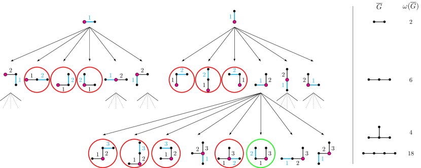
Figure 1: Enumeration of graphs on a lattice: example of the square lattice. We depart from each link in the unit cell. In the red-circled graphs, the newly added link (in cyan) has not the smallest possible label. Such a graph has no children and only its double with the smallest label, child of another parent, is allowed to breed. The green circle highlights a graph, which is kept, although the label of its new link is 2 instead of 1. But the link of label 1 is a bridge, which cannot have been added to a parent (an orphan link). On the right are recapitulated the topological graphs and their occurence numbers.

This part of the calculation consists in finding all relevant simple connected graphs $G$ (those appearing on the considered lattice) and calculating their weight $w(G)$. This is not the main subject of this article, but for completeness, we present here an algorithm that do the job and has the advantage of being parallelizable, as well as two ways of sparing time in some specific situations. It is mathematically described in [23]. A directed tree is constructed, whose vertices are graphs on the lattice (in fact, classes of translation-equivalent graphs). Graphs of the $n$’th generation have $n$ links, and each branch of the tree can be explored independently, as we are able to decide if we keep or not a vertex without exploring the tree (see Fig. 1). The root of the tree is the empty graph. The first generation vertices are all the one-link graphs contained in a unit cell (translationally inequivalent). The next generations are constructed as follows:

• For a graph $G$ with $n-1$ links embedded on the lattice, we consider all the simple graphs with $n$ links obtained by adding an adjacent link to $G$.

• We want to keep only one among all identical (up to a translation) graphs obtained from all $G$’s. For this, the $n$ links of each child $G^{\prime}$ are labelled in a way that only depends on $G^{\prime}$ and not of its parent (ordering the coordinates of its sites for example). Thus, for each copy, the label of the new link is different. Note that bridges of $G^{\prime}$ are orphan links, meaning that they and they alone cannot be new links. We keep $G^{\prime}$ only if the new link has the smallest label among the non-orphan links.

• For each graph $G$ (each vertex of the tree), a canonical label $\overline{G}$ is calculated, such that two isomorphic graphs (identical up to a vertex renumbering) have the same canonical label. It uses the McKay’s algorithm[24, 25]. All graph isomorphism classes are collected and their occurrence number $w(\overline{G})$ (also called the lattice constant, or weak embedding constant) is counted.

Note that different methods, said more efficient but not implemented in our code, are described in the literature[26, 13]. They consist roughly in first generating all topological classes of graphs (this step itself can be realized in different ways), and secondly in counting their embedding number on the lattice. It avoids the costly step of the canonical label calculation, that is however reduced in our algorithm using the two following tricks.

2.4.1 Avoid the canonical labelling of graphs with leaves

The calculation of canonical labels in the last step of the graph enumeration is expensive. When all sites of the lattice have the same number of neighbors $z$, we can spare time by avoiding to calculate it for graphs with leaves (see App. A for the definition of a leaf), as the multiplicity of their topological graph can be deduced as follows. Let $\overline{G}$ be a topological connected simple graph containing a leaf $l=v\leftrightarrow w$ with $d^{\circ}v>d^{\circ}w=1$. Let $n_{a}(\overline{G})$ be the number of automorphisms of $\overline{G}$, i.e. the number of permutations of sites of $\overline{G}$, which map links on links. This number is a by-product of McKay’s algorithm. Let $n_{e}(\overline{G})=n_{a}(\overline{G})w(\overline{G})$. This is the number of embeddings (injective mappings of sites and links) of $\overline{G}$ into the lattice (per unit cell). In other words $w(\overline{G})$ counts subgraphs of lattice isomorphic to $\overline{G}$, whereas $n_{e}(\overline{G})$ counts isomorphisms between $\overline{G}$ and subgraphs of the lattice. $w(\overline{G})$ is deduced from:

$$n_{e}(\overline{G})=(z-d^{\circ}v+1)\,n_{e}(\overline{G}\setminus l)-\sum_{\begin{subarray}{c}s{\rm~{}site~{}of~{}}\overline{G}\\ s\neq v,\,v\leftrightarrow s\,\notin\overline{G}\end{subarray}}n_{e}(\overline{G}\cup\{v\leftrightarrow s\}\setminus l),$$ (19)

requiring only the calculation of $n_{a}$ for the graphs appearing in the formula. Needed $w$ are known if we calculate $w(\overline{G})$ in ascending order of $N_{s}(\overline{G})$.

Example:

We apply formula (19) to calculate $w(\includegraphics[trim=0.0pt 2.00749pt 0.0pt 0.0pt,width=42.67912pt]{linearn3})$ on a triangular lattice. We know $n_{a}(\includegraphics[trim=0.0pt 2.00749pt 0.0pt 0.0pt,width=28.45274pt]{linearn2})=n_{a}(\includegraphics[trim=0.0pt 2.00749pt 0.0pt 0.0pt,width=42.67912pt]{linearn3})=2$, $n_{a}(\includegraphics[trim=0.0pt 6.02249pt 0.0pt 0.0pt,width=15.6491pt]{triangle})=6$, $w(\includegraphics[trim=0.0pt 2.00749pt 0.0pt 0.0pt,width=28.45274pt]{linearn2})=3+6+6=15$ (for links respectively at 0, 60 and at 120 degrees on the lattice) and $w(\includegraphics[trim=0.0pt 6.02249pt 0.0pt 0.0pt,width=15.6491pt]{triangle})=2$.

$$n_{e}(\includegraphics[trim=0.0pt 2.00749pt 0.0pt 0.0pt,width=42.67912pt]{linearn3})=(6-2+1)n_{e}(\includegraphics[trim=0.0pt 2.00749pt 0.0pt 0.0pt,width=28.45274pt]{linearn2})-n_{e}(\includegraphics[trim=0.0pt 6.02249pt 0.0pt 0.0pt,width=15.6491pt]{triangle})$$

$$\Rightarrow w(\includegraphics[trim=0.0pt 2.00749pt 0.0pt 0.0pt,width=42.67912pt]{linearn3})=69.$$

Remark:

The time saved this way is important, as graphs with leaves are the majority when the number of links and the lattice dimensionality increases. In the case of a $d-$dimensional hypercubic lattice[27], $w(\overline{G})=O((2d-1)^{N_{l}})$ for a tree of $N_{l}$ bonds in the limit of large $d$, whereas a topological graph with a loop of $2s$ sites has $w(\overline{G})=O((2d-1)^{N_{l}-s})$.

When adding a link to a connected graph, no more than two leaves may disappear. Hence we can prune a graph $G$ with more than $2(n-\#G)$ leaves.

2.4.2 Expansion in the magnetic field $B$: non-contributing graphs

We have seen in Sec. 2.1 an elegant way to get HTSEs which include all orders in the magnetic field $B$, through expansion coefficients that are even polynomials in $\theta$ (fixed-$\theta$ expansion). However, most physical studies are performed at fixed $B$, requiring either to expand the fixed-$\theta$ expansion coefficients of Eq. (10) in powers of $\beta$, or to directly work with the fixed-$B$ expansion of Eq. (6). Final coefficients are of course the same in both cases, and coefficients in $\beta^{l}$ are even polynomials in $B$ of maximal order $l$.

To get the fixed-$B$ expansion of $F(G)$ for a graph $G$ up to order $\beta^{n}$ from the fixed-$\theta$ expansion, the polynomial coefficient $P_{l}(\theta)$ of the $\beta^{l}$ term of the latter can be truncated at order $k=n-l$ in $\theta$, but it generally does not bring a lot, except in some cases where $P_{l}(\theta)$ is divisible by $\theta^{k+1}$. Then, the graph $G$ can simply be discarded. Here are some simple situations where it occurs:

1. For $B=0$, a graph $G$ with $k$ links that are either bridges or leaves can be discarded if $\#G+k>n$.

2. A graph $G$ with $k$ big leaves (see App. A) does not contribute to the fixed-$B$ expansion at order $n$ if $\#G+k>n$.

The proofs are in App. C (they use some formulae derived in the following sections), together with other, better criteria.

2.5 Complexity and bottleneck of HTSE

We now evaluate the complexity of calculating $F(G)$ up to order $n$. In the sequel $J_{l}$’s may all have the same value, or several values (for example first and second neighbor interactions). But for simplicity, time complexity estimates will all assume $J_{l}$s are all equal. For instance a polynomial of degree $n$ in $\theta$, $J_{1}$, $J_{2},\ldots,J_{k}$ has $O(n^{1+k})$ coefficients. Multiplication of two such polynomials takes time $O(n^{2+2k})$. In the sequel, this estimate will always be $O(n^{4})$. The calculation of $F(G)$ divides in three successive steps, whose complexity is given here and proved in App. D:

• Get the averages $\llangle\hat{H}_{J}^{k}\rrangle$ for $k\leq n$, in a time $O(4^{N_{s}}nN_{l}/\sqrt{N_{s}})$. According to Eq. (11) we have $\overline{g}(G)$ at order $n$.

• Calculate $g(G)$ as $\ln\overline{g}(G)$ at order $n$ in a time $O(n^{4}N_{s})$,

• From $g(G)$ and $F(G^{\prime})$ for $G^{\prime}\subsetneq G$, calculate $F(G)$ using Eq. (16) in a time $O(2^{N_{l}}n^{2})$, or better in a time $O(N_{l}^{2}n^{2})$ as explained in App. D.1.

Finally, the bottleneck to get $F(G)$ at order $n$ among the three steps listed above is the calculation of averages in $O(4^{N_{s}}nN_{l}/\sqrt{N_{s}})$. Then, at fixed $n$, the most greedy graphs are those with the largest $N_{s}$. As the considered graphs are connected, $N_{s}\leq 1+N_{l}\leq n+1$. For $n$ fixed, the way to maximize $N_{s}$ is to choose $N_{l}=n$ and to forbid loops ($N_{s}=1+N_{l}$), which results in graphs that are trees with $n$ links.

The next section describes a way to calculate $F(G)$ in a considerably faster time $O(n^{2})$, for bridged graphs with $N_{l}=n$ links (which include all trees except the star graph $T_{n}$ of Fig. 2), assuming that we know $F(G^{\prime})$ for any simple graph $G^{\prime}\subsetneq G$.

3 $O(n^{2})$ complexity for $n$ links bridged graphs and order $n$ expansion

Let $G$ be a simple connected graph with $N_{l}=\#G$ links. According to Eq. (14), $F(G)=J^{G}\llbracket G\rrbracket+o(J^{G})$ and cumulant $\llbracket G\rrbracket$ is derived from moments of subgraphs of $G$ by

$$\llbracket G\rrbracket =\sum_{q\in Q(G)}g_{0}(\#q)\prod_{G^{\prime}\in q}\llangle G^{\prime}\rrangle,$$ (20)

$$g_{0}(i) =(-1)^{i-1}(i-1)!=(-1)(-2)\cdots(1-i),$$ (21)

where $Q(G)$ is the set of partitions of $G$ and $\#q$ is the cardinal of the partition $q$. This equation is proved in appendix (B) as Eq. (B.13).

In this section, we demonstrate that if $G$ is a bridged graph (an undirected graph that can be split in two connected components by removing a single link), $F(G)$ can be calculated at order $n=\#G$ in $J$, in time $O(n^{2})$, if we know $F(G^{\prime})$ for any connected subgraph $G^{\prime}\subsetneq G$.

We choose a bridge of $G$ that we denote $u\leftrightarrow v$. Let $U$ and $V$ be the two connected components of $G\setminus\{u\leftrightarrow v\}$. We assume that $u$ is a site of $U$ and $v$ is a site of $V$.

We now prove the first main result of this article:

$$\llbracket G\rrbracket=\llbracket U,u\leftrightarrow v,V\rrbracket=\frac{2}{\theta^{2}}\llbracket U,u\leftrightarrow v\rrbracket\llbracket u\leftrightarrow v,V\rrbracket,$$ (22)

But we will first prove forecoming Eq. (26). Operator $\hat{P}_{u\leftrightarrow v}$ exchanges spins of sites $u$ and $v$ of link $u\leftrightarrow v$. So

$$\hat{P}_{u\leftrightarrow v}=\hat{p}^{{+}{+}}_{u}\hat{p}^{{+}{+}}_{v}+\hat{p}^{{+}{-}}_{u}\hat{p}^{{-}{+}}_{v}+\hat{p}^{{-}{+}}_{u}\hat{p}^{{+}{-}}_{v}+\hat{p}^{{-}{-}}_{u}\hat{p}^{{-}{-}}_{v},$$ (23)

where operator $\hat{p}^{{\epsilon}{\epsilon^{\prime}}}_{s}$ transforms state $\epsilon$ of spin $S^{z}_{s}$ into state $\epsilon^{\prime}$. We define

$$\llbracket U\rrbracket^{+}_{u}\,=\llbracket U,\hat{p}^{{+}{+}}_{u}\rrbracket,\qquad\llbracket U\rrbracket^{-}_{u}\,=\llbracket U,\hat{p}^{{-}{-}}_{u}\rrbracket$$ (24)

The trace of an operator which decreases total spin $S^{z}$ on the sites of $U$, is zero. Hence $\llangle G^{\prime},\hat{p}^{{+}{-}}_{u}\hat{p}^{{-}{+}}_{v}\rrangle=0$ for any subgraph $G^{\prime}\subset U\cup V$. Hence $\llbracket U,\hat{p}^{{+}{-}}_{u}\hat{p}^{{-}{+}}_{v},V\rrbracket=0$. When computing moment or cumulant of a graph $G$ with a leaf ($U$ or $V$ being empty) or bridge $u\leftrightarrow v$ we can replace $\hat{P}_{u\leftrightarrow v}$ by $\hat{p}^{{+}{+}}_{u}\hat{p}^{{+}{+}}_{v}+\hat{p}^{{-}{-}}_{u}\hat{p}^{{-}{-}}_{v}$. Sum of both projections on the possible states of a spin is identity, which is independent with any operator. Hence if $U$ is a non-empty graph: $\llbracket U\rrbracket^{+}_{u}\,+\llbracket U\rrbracket^{-}_{u}\,=\llbracket U,\hat{p}^{{+}{+}}_{u}\rrbracket+\llbracket U,\hat{p}^{{-}{-}}_{u}\rrbracket=\llbracket U,\hat{p}^{{+}{+}}_{u}+\hat{p}^{{-}{-}}_{u}\rrbracket=\llbracket U,\mathbf{\hat{I}}\rrbracket=0$. For an empty graph: $\llbracket\emptyset\rrbracket^{+}_{u}\,=\llbracket\hat{p}^{{+}{+}}_{u}\rrbracket=\llangle\hat{p}^{{+}{+}}_{u}\rrangle=\theta_{+}$ i.e. probability for a isolated spin to be in $+$ state.

$$U\neq\emptyset\Rightarrow\llbracket U\rrbracket^{-}_{u}\,=-\llbracket U\rrbracket^{+}_{u}\,,\quad\llbracket\emptyset\rrbracket^{+}_{u}\,=\theta_{+},\quad\llbracket\emptyset\rrbracket^{-}_{u}\,=\theta_{-}.$$ (25)

Links in $U$ and $\hat{p}^{{\epsilon}{\epsilon}}_{u}$ operate on spins of sites of $U$. These operators commute with those of $V$. With equation Eq. (B.7) and linearity of cumulants we have

$$\llbracket U,u\leftrightarrow v,V\rrbracket =\llbracket U,\!\sum_{\epsilon\in\{+,-\}}\!\hat{p}^{{\epsilon}{\epsilon}}_{u}\hat{p}^{{\epsilon}{\epsilon}}_{v},V\rrbracket$$

$$=\!\sum_{\epsilon\in\{+,-\}}\!\llbracket U,\hat{p}^{{\epsilon}{\epsilon}}_{u}\rrbracket\llbracket\hat{p}^{{\epsilon}{\epsilon}}_{v},V\rrbracket$$

$$=\llbracket U\rrbracket^{+}_{u}\,\llbracket V\rrbracket^{+}_{v}\,+\llbracket U\rrbracket^{-}_{u}\,\llbracket V\rrbracket^{-}_{v}\,.$$ (26)

With an empty $V$, this equation becomes

$$\llbracket U,u\leftrightarrow v\rrbracket=\llbracket U\rrbracket^{+}_{u}\,\theta_{+}+\llbracket U\rrbracket^{-}_{u}\,\theta_{-}=\llbracket U\rrbracket^{+}_{u}\,(\theta_{+}-\theta_{-})=\llbracket U\rrbracket^{+}_{u}\,\theta.$$ (27)

Similarly with an empty $U$ it becomes $\llbracket u\leftrightarrow v,V\rrbracket=\llbracket V\rrbracket^{+}_{v}\,\theta$. Otherwise it becomes

$$\llbracket G\rrbracket=\llbracket U\rrbracket^{+}_{u}\,\llbracket V\rrbracket^{+}_{v}\,-\llbracket U\rrbracket^{+}_{u}\,(-\llbracket V\rrbracket^{+}_{v}\,)=2\llbracket U\rrbracket^{+}_{u}\,\llbracket V\rrbracket^{+}_{v}\,.$$ (28)

Elimination of $\llbracket U\rrbracket^{+}_{u}\,$ and $\llbracket V\rrbracket^{+}_{v}\,$ between these three equations gives Eq. (22).

Search for bridge $u\leftrightarrow v$ and subgraphs $U$ and $V$ in graph $G$ takes time $O(n)$. Retrieval of $\llbracket U,u\leftrightarrow v\rrbracket$ as coefficient of $J^{U}J_{u\leftrightarrow v}$ in $F(U\cup\{u\leftrightarrow v\})$ takes time $O(n)$, since $\llbracket U,u\leftrightarrow v\rrbracket\in\mathbb{Q}_{1+N_{l}(U)}[\theta^{2}]$. Multiplication of polynomials $\llbracket U,u\leftrightarrow v\rrbracket$ and $\llbracket u\leftrightarrow v,V\rrbracket/\theta^{2}$ takes time $O(n^{2})$. So overall time to compute $\llbracket G\rrbracket$ is $O(n^{2})$.

4 Trees with $n$ links

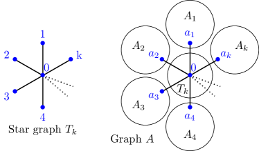
Figure 2: Left: star graph $T_{k}$. Right: graph $A$ used in Sec.4, where the $A_{i}$ subgraphs are non-empty.

We show in this section the second main result of this article: for a tree $T$ with $N_{l}\geq 2$:

$$\llbracket T\rrbracket=\frac{1}{2}\prod_{s\,\in\,\textrm{ sites of }T}2C_{d^{\circ}s},$$ (29)

where $d^{\circ}s$ is the number of links departing from site $s$, and $C_{k}$ is recursively defined by:

$$C_{1}=\frac{\theta}{2},\qquad\qquad C_{k+1}=\frac{dC_{k}}{dh}=\frac{1-\theta^{2}}{2}\,\frac{dC_{k}}{d\theta}.$$ (30)

Value of $C_{1}$ is given by equations (22) and (29): When joining trees $U$ and $V$ to build tree $G$, one tree and two leaves disappear. Hence $\frac{1}{2}(2C_{1})^{2}=\frac{\llbracket U\rrbracket\llbracket V\rrbracket}{\llbracket G\rrbracket}=\frac{\theta^{2}}{2}$. We get values of $C_{k}$ for $k>1$ by applying Eq. (29) to a star graph $T_{k}=\{0\leftrightarrow 1,0\leftrightarrow 2,\dots,0\leftrightarrow k\}$ (Fig. 2, left).

$$\llbracket T_{k}\rrbracket=C_{k}\theta^{k}.$$ (31)

It remains to prove Eq. (30). For this we consider a graph $A$ that possesses $k$ links originating from a site $\mathrm{𝟎}$, namely ${0\leftrightarrow a_{1},0\leftrightarrow a_{2},\dots,0\leftrightarrow a_{k}}$. These links may be either bridges or leaves. We denote $A_{1}$, $A_{2}$, …$A_{k}$ the $k$ components of $A$ containing sites $a_{1}$, $a_{2}$,…$a_{k}$, obtained by cutting these links (see Fig. 2, right). If in $\llbracket A\rrbracket$ we replace every $\hat{P}_{0\leftrightarrow a_{i}}$ by $\hat{p}^{{+}{+}}_{0}\hat{p}^{{+}{+}}_{a_{i}}+\hat{p}^{{-}{-}}_{0}\hat{p}^{{-}{-}}_{a_{i}}$ and use multilinearity of cumulant and Eq. (B.7) as we did to get Eq. (26), we get:

$$\llbracket A\rrbracket=\sum_{\varepsilon\in\{+,-\}^{k}}\llbracket\hat{p}^{{\varepsilon_{1}}{\varepsilon_{1}}}_{0},\ldots,\hat{p}^{{\varepsilon_{k}}{\varepsilon_{k}}}_{0}\rrbracket\prod_{i=1}^{k}\llbracket A_{i}\rrbracket^{\varepsilon_{i}}_{a_{i}}\,$$ (32)

There we replace every $\hat{p}^{{-}{-}}_{0}=\mathbf{\hat{I}}-\hat{p}^{{+}{+}}_{0}$ by $-\hat{p}^{{+}{+}}_{0}$ and get:

$$\llbracket A\rrbracket=\llbracket\hat{p}^{{+}{+}}_{0}{}^{(k)}\rrbracket\prod_{i=1}^{k}(\llbracket A_{i}\rrbracket^{+}_{a_{i}}\,-\llbracket A_{i}\rrbracket^{-}_{a_{i}}\,).$$ (33)

If all $A_{i}$’s are empty we get $\llbracket T_{k}\rrbracket=\llbracket(\hat{p}^{{+}{+}}_{0})^{(k)}\rrbracket\theta^{k}$. Hence $C_{k}=\llbracket(\hat{p}^{{+}{+}}_{0})^{(k)}\rrbracket$. But

$$\llangle e^{\lambda\hat{p}^{{+}{+}}_{0}}\rrangle=\llangle e^{\lambda}\hat{p}^{{+}{+}}_{0}+\hat{p}^{{-}{-}}_{0}\rrangle=\frac{e^{\lambda+h/2}+e^{-h/2}}{Y},$$

and Eq. (B.4) give (for $k>1$):

$$C_{k}&=\llbracket\hat{p}^{{+}{+}}_{0}{}^{(k)}\rrbracket=\frac{\partial^{k}}{\partial\lambda^{k}}\ln\frac{e^{\lambda+\frac{h}{2}}+e^{-\frac{h}{2}}}{Y}\Big{|}_{\lambda=0}\\ =\frac{\partial^{k}}{\partial\lambda^{k}}\ln\cosh\frac{\lambda+h}{2}\Big{|}_{\lambda=0}=\frac{d^{k}}{dh^{k}}\ln\cosh\frac{h}{2}\\ =\frac{1}{2}\frac{d^{k-1}}{dh^{k-1}}\tanh\frac{h}{2}=\frac{d^{k-1}}{dh^{k-1}}\,\frac{\theta}{2}$$ (34)

Eq. (34) for all $k\geq 1$ is equivalent to whole Eq. (30). But Eq. (34) holds only for $k>1$. For $k=1$ it gives the wrong value $C_{1}=\theta_{+}$.

Formulae (29) and (30) allow for a calculation in $O(n^{2})$ of $F(T)$ for any tree $T$ with $n$ links, to be compared with the $O(4^{n}n^{3/2})$ of the usual method.

5 Discussion and conclusion

We have reviewed the two steps involved in the exact calculation of HTSE coefficients for Heisenberg $S=1/2$ spin lattices, in the presence of a magnetic field ($i$) the graph enumeration and ($ii$) the trace calculation. We gave evidence that the trace calculations on bridged graphs (and particularly on trees) with $n$ links are the most time consuming steps, with a complexity in $O(n^{3/2}2^{n})$, and derived formulae that drastically decrease it to $O(n^{2})$.

An optimized and parallelized code using this optimization is available as Supp. Mat[21]. The time required by this code for the two main steps (graph enumeration and trace calculations) are recapitulated in App. D.4 for some number of CPUs and for some simple models. This code was used and perfected in articles on the kagome anti-ferromagnet by the authors[5, 6] in the presence of a magnetic field, but also on many other models without magnetic field[11, 8, 7]. Actually, the code allows also to calculate HTSE for models with anisotropic interactions and Dzyaloshinskii-Moriya interactions.

Further studies could extend this work to optimize HTSE calculation on a larger class of models (different spin values, classical models) in the presence of a magnetic field. Moreover, some of the authors are presently working on various ways to exploit the knowledge of the field dependent HTSE coefficients, by considering other thermodynamic ensemble than the more usually used $(T,B)$, as evoked in Sec. 2.1.

Funding information

This work was supported by the French Agence Nationale de la Recherche under Grant No. ANR-18-CE30-0022-04 LINK and the projet Emergence, of the Paris city.

Appendix A Vocabulary on graphs

All the definitions below are illustrated on Fig. 3.

Graphs where each link appears only once are called simple graphs, and graphs where multiple links are allowed are called multi-graphs.

A graph is connected when a path exists between any two of its sites (it has only one connected component).

The degree $d^{\circ}s$ of a site $s$ is the number of links emanating from it.

A leaf is a link with a site of degree one.

A bridge is a link that is not a leaf and belongs to no simple loop. So it connects two otherwise not connected components. A graph with a bridge is said bridged.

A big leaf is a generalization of a leaf. If not a leaf it is a bridge in company of one of the two components it separates, provided this component is free of leaves or bridges. So no big leaf can include another one. That is why all big leaves are disjoint, except when there is only one bridge and no leaf. Then there are two big leaves sharing the only bridge and we must pretend there is only one big leaf. This way big leaves are always disjoint as needed. Let $N_{bl}$ be the total number of bridges and leaves. Let $N_{L}$ be the (pretended) number of big leaves. Then $\mathrm{min}(N_{bl},2)\leq N_{L}\leq N_{bl}$.

An islet of a graph $G$ is a connected component of the graph obtained after cutting every bridge of $G$ and replacing it by two leaves.

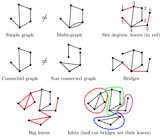
Figure 3: Some definitions on graphs

Appendix B Averages, moments and cumulants

The moment and cumulant of a multiset or list of operators $\hat{x}_{1},\ldots,\hat{x}_{k}$ are:

$$\langle\hat{x}_{1},\ldots,\hat{x}_{k}\rangle =\frac{\partial}{\partial\lambda_{1}}\cdots\frac{\partial}{\partial\lambda_{k}}\left\langle e^{\sum_{i=1}^{k}\lambda_{i}\hat{x}_{i}}\right\rangle\Big{|}_{\lambda=0}$$ (B.1)

$$=\frac{1}{k!}\sum_{\sigma\in S_{k}}\left\langle\prod_{i=1}^{k}\hat{x}_{\sigma(i)}\right\rangle,$$ (B.2)

$$[\hat{x}_{1},\ldots,\hat{x}_{k}] =\frac{\partial}{\partial\lambda_{i}}\cdots\frac{\partial}{\partial\lambda_{k}}\ln\left\langle e^{\sum_{i}\lambda_{i}\hat{x}_{i}}\right\rangle\Big{|}_{\lambda=0}.$$ (B.3)

For a single operator $\hat{x}_{1}$, moment $\langle\hat{x}_{1}\rangle$, cumulant $[\hat{x}_{1}]$ and average $\langle\hat{x}_{1}\rangle$ are equal. So we can use notation $\langle.\rangle$ for both average and moment. Furthermore $\langle\hat{x}^{(k)}\rangle=\langle\hat{x}^{k}\rangle=[\hat{x}^{k}]\neq[\hat{x}^{(k)}]$ for $k>1$ if $\hat{x}^{(k)}$ denotes $k$ occurences $\hat{x},\ldots,\hat{x}$ of a same operator.

If $\hat{x}_{i}=\hat{x}_{j}$ in definitions B.1 and B.3 we can state $\mu=\lambda_{i}+\lambda_{j}$. Then $\partial\mu/\partial\lambda_{i}=\partial\mu/\partial\lambda_{j}=1$. Hence we can replace $\lambda_{i}\hat{x}_{i}+\lambda_{j}\hat{x}_{j}$ by $\mu\hat{x}_{i}$ and both $\partial\lambda_{i}$ and $\partial\lambda_{j}$ by $\partial\mu$. More simply we can remove term $\lambda_{j}\hat{x}_{j}$ in sum and replace $\partial\lambda_{j}$ by $\partial\lambda_{i}$. In this way we have for instance:

$$[\hat{x}_{1}^{(3)},\hat{x}_{2},\hat{x}_{3}^{(4)}]={\partial^{3}\over\partial\lambda_{1}^{3}}\frac{\partial}{\partial\lambda_{2}}{\partial^{4}\over\partial\lambda_{3}^{4}}\ln\langle e^{\sum_{i=1}^{3}\lambda_{i}\hat{x}_{i}}\rangle\Big{|}_{\lambda=0}.$$ (B.4)

We now consider that $\hat{x}$ is an operator corresponding to a link $x$ of a graph. Note that we use from now on the vocabulary of graphs using this operator-link correspondance, but that what follows is valid for any set or multiset of operators. Hence if $G$ is a simple graph, i.e. a set of distinct links, we have Maclaurin expansion

$$\ln\langle\exp\sum_{x\in G}\lambda_{x}\hat{x}\rangle=\sum_{U\in{\mathbb{N}^{G}}}\frac{[\hat{x}^{(U(x))},x\in G]}{\prod_{x\in G}U(x)!}\prod_{x\in G}\lambda_{x}^{U(x)}.$$ (B.5)

Here $U\in{\mathbb{N}^{G}}$ is a mapping from $G$ to $\mathbb{N}$. For each link $x\in G$, integer $U(x)$ is its multiplicity in the multiset $\{\!\!\{x^{(U(x))},x\in G\}\!\!\}$. So $U$ is any multigraph whose support is a part of $G$. We will simplify notations in this last equation and rewrite it:

$$\ln\langle\exp\lambda G\rangle=\sum_{U\in{\mathbb{N}^{G}}}\frac{[U]}{U!}\lambda^{U}=\sum_{k=1}^{\infty}\sum_{V\in G^{k}}{[V]\over k!}\lambda^{V}.$$ (B.6)

Instead of summing over multisets of links, we may sum over tuples of links. But a multiset $U\in\mathbb{N}^{G}$ of $k=\#U=\sum_{x\in G}U(x)$ links appears $k!/U!$ times among tuples ${V\in G^{k}}$ of $k$ links. Similarly we have also

$$\langle\exp\lambda G\rangle=\sum_{U\in{\mathbb{N}^{G}}}\frac{\langle U\rangle}{U!}\lambda^{U}=1+\sum_{k=1}^{\infty}\sum_{V\in G^{k}}{\langle V\rangle\over k!}\lambda^{V}.$$ (B.7)

The constant coefficients of these series in powers of $\lambda$ are $\langle\emptyset\rangle=\langle e^{0}\rangle=1$ and $[\emptyset]=\ln 1=0$. So coefficients of either of these two formal series can be computed from the coefficients of the other one by

$$\sum_{U\in{\mathbb{N}^{G}}}{\langle U\rangle\over U!}\lambda^{U} =1+\sum_{n=1}^{\infty}\left(\sum_{U\in{\mathbb{N}^{G}}}{[U]\over U!}\lambda^{U}\right)^{n}/n!,$$ (B.8)

$$\sum_{U\in{\mathbb{N}^{G}}}{[U]\over U!}\lambda^{U} =-\sum_{n=1}^{\infty}\left(1-\sum_{U\in{\mathbb{N}^{G}}}{\langle U\rangle\over U!}\lambda^{U}\right)^{n}/n.$$ (B.9)

B.1 Moments expressed as polynomials of cumulants

For a simple graph $U=\{x_{1},\ldots,x_{k}\}$ the coefficient of $\lambda^{U}$ in Eq. (B.8) is

$$\langle U\rangle=\sum_{p\in Q(U)}\prod_{G\in p}[G],$$ (B.10)

where $Q(U)$ is the set of partitions of $U$. Divisions by $U!=1$ and $G!=1$ disappear, since graph $U$ and its part $G$ are simple. Furthermore division by $n!$ disappears also because the product of the cumulants of the $n$ parts of a partition $p$ appears $n!$ times with reordered factors within $\big{(}\cdots\big{)}^{n}$.

To generalize this formula to multigraphs, we no more use partitions of sets of links, but partitions of set $\{1,\ldots,n\}$ so that links $x_{i}$ no longer need be different:

$$\langle\hat{x}_{1},\ldots,\hat{x}_{n}\rangle=\sum_{p\in Q(n)}\prod_{q\in p}[\hat{x}_{r},r\in q].$$ (B.11)

$Q(n)$ is the set of partitions of set $\{1,\dots,n\}$.
Example:

$$\langle\hat{x}_{1},\hat{x}_{2},\hat{x}_{3}\rangle=[\hat{x}_{1},\hat{x}_{2},\hat{x}_{3}]+[\hat{x}_{1},\hat{x}_{2}][\hat{x}_{3}]+[\hat{x}_{1},\hat{x}_{3}][\hat{x}_{2}]+[\hat{x}_{1}][\hat{x}_{2},\hat{x}_{3}]+[\hat{x}_{1}][\hat{x}_{2}][\hat{x}_{3}].$$

B.2 Cumulants expressed as polynomials of moments

For a simple graph $U=\{x_{1},\ldots,x_{k}\}$ the coefficient of $\lambda^{U}$ in Eq (B.9) is

$$[U]=\sum_{p\in Q(U)}g_{0}(\#p)\prod_{G\in p}\langle G\rangle.$$ (B.12)

When going from Eq. (B.8) to Eq. (B.10), coefficient $1/n!$ disappears when multiplied by $n!$. Here $(-1)^{n-1}/n$ multiplied by $n!$ becomes $g_{0}(n)=(-1)^{n-1}(n-1)!$. For multigraphs we have:

$$[\hat{x}_{1},\ldots,\hat{x}_{n}]=\sum_{p\in Q(n)}g_{0}(\#p)\prod_{q\in p}\langle\hat{x}_{r},r\in q\rangle.$$ (B.13)

Example:

$$[\hat{x}_{1},\hat{x}_{2}]= \langle\hat{x}_{1},\hat{x}_{2}\rangle-\langle\hat{x}_{1}\rangle\langle\hat{x}_{2}\rangle=\langle\hat{x}_{1}\hat{x}_{2}\rangle-\langle\hat{x}_{1}\rangle\langle\hat{x}_{2}\rangle$$

$$[\hat{x}_{1},\hat{x}_{2},\hat{x}_{3}]= \langle\hat{x}_{1},\hat{x}_{2},\hat{x}_{3}\rangle-\langle\hat{x}_{1},\hat{x}_{2}\rangle\langle\hat{x}_{3}\rangle-\langle\hat{x}_{1},\hat{x}_{3}\rangle\langle\hat{x}_{2}\rangle-\langle\hat{x}_{1}\rangle\langle\hat{x}_{2},\hat{x}_{3}\rangle+2\langle\hat{x}_{1}\rangle\langle\hat{x}_{2}\rangle\langle\hat{x}_{3}\rangle.$$

$$= \frac{\langle\hat{x}_{1}\hat{x}_{2}\hat{x}_{3}\rangle+\langle\hat{x}_{1}\hat{x}_{3}\hat{x}_{2}\rangle}{2}-\langle\hat{x}_{1}\hat{x}_{2}\rangle\langle\hat{x}_{3}\rangle-\langle\hat{x}_{1}\hat{x}_{3}\rangle\langle\hat{x}_{2}\rangle-\langle\hat{x}_{1}\rangle\langle\hat{x}_{2}\hat{x}_{3}\rangle+2\langle\hat{x}_{1}\rangle\langle\hat{x}_{2}\rangle\langle\hat{x}_{3}\rangle.$$

B.3 Moment and cumulants of a single operator

When $\hat{x}_{1}=\hat{x}_{2}=\cdots=\hat{x}_{n}=\hat{H}$ equations (B.11) and (B.13) become

$$\langle\hat{H}^{n}\rangle =\sum_{\begin{subarray}{c}n_{1},\dots,n_{n}\in\mathbb{N},\\ \sum_{i}in_{i}=n\end{subarray}}n!\prod_{i}\frac{[\hat{H}^{(i)}]^{n_{i}}}{(i!)^{n_{i}}n_{i}!},$$ (B.14)

$$[\hat{H}^{(n)}] =\sum_{\begin{subarray}{c}n_{1},\dots,n_{n}\in\mathbb{N},\\ \sum_{i}in_{i}=n\end{subarray}}g_{0}(\sum_{i}n_{i})n!\prod_{i}\frac{\langle\hat{H}^{i}\rangle^{n_{i}}}{(i!)^{n_{i}}n_{i}!}.$$ (B.15)

Examples:

$$[\hat{H}]= \langle\hat{H}\rangle$$

$$[\hat{H}^{(2)}]= \langle\hat{H}^{2}\rangle-\langle\hat{H}\rangle^{2}$$

$$[\hat{H}^{(3)}]= \langle\hat{H}^{3}\rangle-3\langle\hat{H}^{2}\rangle\langle\hat{H}\rangle+2\langle\hat{H}\rangle^{3}$$

$$[\hat{H}^{(4)}]= \langle\hat{H}^{4}\rangle-3\langle\hat{H}^{2}\rangle^{2}-4\langle\hat{H}^{3}\rangle\langle\hat{H}\rangle+12\langle\hat{H}^{2}\rangle\langle\hat{H}\rangle^{2}-6\langle\hat{H}\rangle^{4}$$

$$[\hat{H}^{(5)}]= \langle\hat{H}^{5}\rangle-5\langle\hat{H}\rangle\langle\hat{H}^{4}\rangle-10\langle\hat{H}^{2}\rangle\langle\hat{H}^{3}\rangle+20\langle\hat{H}^{3}\rangle\langle\hat{H}\rangle^{2}+30\langle\hat{H}\rangle\langle\hat{H}^{2}\rangle^{2}-60\langle\hat{H}^{2}\rangle\langle\hat{H}\rangle^{3}+24\langle\hat{H}\rangle^{5}$$

$$\langle\hat{H}\rangle= [\hat{H}]$$

$$\langle\hat{H}^{2}\rangle= [\hat{H}^{(2)}]+[\hat{H}]^{2}$$

$$\langle\hat{H}^{3}\rangle= [\hat{H}^{(3)}]+3[\hat{H}^{(2)}][\hat{H}]+[\hat{H}]^{3}$$

$$\langle\hat{H}^{4}\rangle= [\hat{H}^{(4)}]+3[\hat{H}^{(2)}]^{2}+4[\hat{H}^{(3)}][\hat{H}]+6[\hat{H}^{(2)}][\hat{H}]^{2}+[\hat{H}]^{4}$$

$$\langle\hat{H}^{5}\rangle= [\hat{H}^{(5)}]+15[\hat{H}][\hat{H}^{(2)}]^{2}+10[\hat{H}^{(2)}][\hat{H}]^{3}+[\hat{H}]^{5}+5[\hat{H}][\hat{H}^{(4)}]+10[\hat{H}^{(2)}][\hat{H}^{(3)}]$$

$$+10[\hat{H}^{(3)}][\hat{H}]^{2}$$

B.4 Expression of cumulants versus moments and lesser order cumulants

From Eq. (B.10) we can easily derive, if $\hat{x}_{1}\in X$:

$$\langle X\rangle=\sum_{X^{\prime}\subset X\setminus\hat{x}_{1}}[X\setminus X^{\prime}]\langle X^{\prime}\rangle$$ (B.16)

Hence

$$[\hat{x}_{1},\dots,\hat{x}_{n}]=\langle\hat{x}_{1},\dots,\hat{x}_{n}\rangle-\sum_{p\in P_{2}^{\prime\prime}(n)}[\hat{x}_{r},r\in p_{1}]\langle\hat{x}_{r},r\in p_{2}\rangle$$ (B.17)

where $P_{2}^{\prime\prime}(n)$ is the set of partitions of $n$ elements in $2$ non-empty sets, with the conditions that $1$ is in the first set.
Example:

$$[\hat{x}_{1},\hat{x}_{2},\hat{x}_{3}]=\langle\hat{x}_{1},\hat{x}_{2},\hat{x}_{3}\rangle-[\hat{x}_{1},\hat{x}_{2}]\langle\hat{x}_{3}\rangle-[\hat{x}_{1},\hat{x}_{3}]\langle\hat{x}_{2}\rangle-[\hat{x}_{1}]\langle\hat{x}_{2},\hat{x}_{3}\rangle$$

B.5 Nullity of cumulant of a not connected graph

Let $C$ be a not connected graph, without isolated site. Let $A$ be one of its connected component. Let $B=C\setminus A$. Then $A$ and $B$ are two non-empty graphs sharing no sites. So operators $\lambda A=\sum_{x\in A}\lambda_{x}\hat{x}$ and $\lambda B$ are independent. Their exponentials too. The average of their product is the product of their averages. But $\lambda C=\lambda A+\lambda B$. Hence $\ln\langle\exp\lambda C\rangle=\ln\langle\exp\lambda A\rangle+\ln\langle\exp\lambda B\rangle$. So

$$\sum_{U\in{\mathbb{N}^{C}}}{[U]\over U!}\lambda^{U}=\sum_{U\in{\mathbb{N}^{B}}}{[U]\over U!}\lambda^{U}+\sum_{U\in{\mathbb{N}^{A}}}{[U]\over U!}\lambda^{U}$$ (B.18)

If $U$ is a multigraph of support $C$, term $[U]\lambda^{U}/U!$ appears only once in Eq. (B.18) in its left hand side. No other term has same $\lambda^{U}$. Hence $[U]=0$. This proves that the cumulant of a not connected multigraph is zero.

B.6 Multilinearity of moments and cumulants

With Eq. (B.2) we see that moment is a linear function of any of its arguments. Then with Eq. (B.13) we see that cumulant too.

B.7 Product of cumulants of independent sets of operators

$$(\forall X^{\prime}\subset X,~{}\forall Y^{\prime}\subset Y,~{}\langle X^{\prime},Y^{\prime}\rangle=\langle X^{\prime}\rangle\langle Y^{\prime}\rangle)~{}$$

$$\Rightarrow[X][Y]=[\hat{x}_{1}\hat{y}_{1},X\setminus\hat{x}_{1},Y\setminus\hat{y}_{1}]$$ (B.19)

We will prove this by induction on $\#X+\#Y$. We denote $X_{1}=X\setminus\hat{x}_{1}$ and $Y_{1}=Y\setminus\hat{y}_{1}$. We have $\langle X\rangle\langle Y\rangle=\langle X,Y\rangle=\langle x_{1}y_{1},X_{1},Y_{1}\rangle$. Hence using three times Eq. (B.16):

$$\left(\sum_{X^{\prime}\subset X_{1}}[X\setminus X^{\prime}]\langle X^{\prime}\rangle\right)\left(\sum_{Y^{\prime}\subset Y_{1}}[Y\setminus Y^{\prime}]\langle Y^{\prime}\rangle\right)=\sum_{W^{\prime}\subset X_{1}\cup Y_{1}}[\hat{x}_{1}\hat{y}_{1},X_{1}\cup Y_{1}\setminus W^{\prime}]\langle W^{\prime}\rangle$$

$$\sum_{X^{\prime}\subset X_{1}\atop Y^{\prime}\subset Y_{1}}[X\setminus X^{\prime}][Y\setminus Y^{\prime}]\langle X^{\prime}\rangle\langle Y^{\prime}\rangle=\sum_{X^{\prime}\subset X_{1}\atop Y^{\prime}\subset Y_{1}}[\hat{x}_{1}\hat{y}_{1},X_{1}\setminus X^{\prime},Y_{1}\setminus Y^{\prime}]\langle X^{\prime}\rangle\langle Y^{\prime}\rangle.$$

According to induction hypothesis, all terms for $X^{\prime}\neq\emptyset$ or $Y^{\prime}\neq\emptyset$ cancel. Only remains what we want to prove.

Appendix C Proof of the non contribution of some graphs in the fixed-$B$ expansion

If $U$ is a connected multigraph with $N_{L}$ big leaves:

$$\theta^{N_{L}(U)}{\rm~{}divides~{}}\llbracket U\rrbracket$$ (C.1)

We assume a multiple link cannot be a leaf or a bridge. Let $k=N_{L}$. Let $A_{1},\ldots,A_{k}$ be the parts of $U$ which are disconnected when removing the leaves or bridges of the big leaves. Let $B=U\setminus A_{1}\setminus A_{2}\setminus\cdots\setminus A_{k}$. A big leaf is $A_{i}\cup\{a_{i}\leftrightarrow b_{i}\}$ with $a_{i}$ in $A_{i}$ and $b_{i}$ in $B$. Then, the very same proof of Eq. (33) gives:

$$\llbracket U\rrbracket=\llbracket B,\hat{p}^{{+}{+}}_{b_{1}},\ldots,\hat{p}^{{+}{+}}_{b_{k}}\rrbracket\prod_{i=1}^{k}(\llbracket A_{i}\rrbracket^{+}_{a_{i}}\,-\llbracket A_{i}\rrbracket^{-}_{a_{i}}\,).$$ (C.2)

Replacing $\theta$ by $-\theta$ in $\llbracket A_{i}\rrbracket^{+}_{a_{i}}\,$ gives $\llbracket A_{i}\rrbracket^{-}_{a_{i}}\,$. Hence $\llbracket A_{i}\rrbracket^{+}_{a_{i}}\,-\llbracket A_{i}\rrbracket^{-}_{a_{i}}\,$ is an odd polynomial in $\theta$ and it is divisible by $\theta$. This proves Eq. (C.1).

C.1 Graphs with $n<N_{l}+N_{bl}$ for $B=0$

We prove here the first item of Sec. 2.4.2: for $B=0$, a graph $G$ with $k=N_{bl}$ links that are either bridges or leaves can be discarded if $\#G+k>n$, because $F(G)=o(\beta^{n})$. Let $U$ be a multi-graph $U$ of support $G$. If $\#U\geq\#G+k$, then $\#U>n$ and $J^{U}=o(\beta^{n})$. Otherwise $\#U<\#G+k$. Doubling $\#U-\#G$ links will disable at most as many bridges or leaves. But at least one will remain. Hence $U$ has a big leaf, and $\llbracket U\rrbracket$ is divisible by $\theta$, meaning since $\theta=0$ that $\llbracket U\rrbracket=0$.

C.2 Graphs with $n<N_{l}+N_{L}$ in fixed-$B$ expansion

Now we count only leaves and bridges inside big leaves to prove the second item of Sec. 2.4.2: A graph $G$ with $N_{L}$ big leaves does not contribute to the fixed-$B$ expansion at order $n$ if ${\#G+N_{L}>n}$. Let $U$ be a multi-graph of support $G$. Then $\theta^{N_{L}(U)}$ divides $\llbracket U\rrbracket$. Hence

$$\mathrm{order}_{\beta}\frac{J^{U}\llbracket U\rrbracket}{U!}~{}\geq~{}\#U+N_{L}(U)~{}\geq~{}\#G+N_{L}(G)~{}>~{}n$$

C.3 Better criteria in fixed-$B$ expansion

We now explain a better criterium (C.5), and give an algorithm to compute it.

For this, we define odd islets and count them with big leaves. In a connected graph $G$ with $N_{b}$ bridges, we can replace every bridge $l=l_{1}\leftrightarrow l_{2}$ by two leaves $l_{1}\leftrightarrow l_{4}$ and $l_{3}\leftrightarrow l_{2}$ where $l_{3}$ and $l_{4}$ are $2N_{b}$ new sites. We get $N_{b}+1$ connected components, that we call islets (see App. A). An islet will be said odd if it has an odd number of leaves. We denote $N_{o}(G)$ the number of odd islets of $G$. We denote $U_{0},$ $U_{1}\dots U_{N_{b}}$ the islets of $G$. We denote $N_{f}(G)$ the number of leaves of $G$. Eq. (C.1) tells us that $\theta^{N_{f}(G)}$ divides $\llbracket G\rrbracket$ and $\theta^{N_{f}(U_{i})}$ divides $\llbracket U_{i}\rrbracket$. This is coherent with $N_{f}(G)=\sum_{i=0}^{N_{b}}N_{f}(U_{i})-2N_{b}$ and $\llbracket G\rrbracket=(2/\theta^{2})^{N_{b}}\prod_{i}\llbracket U_{i}\rrbracket$. But $\llbracket U_{i}\rrbracket$ is an even polynomial of $\theta$. So when $U_{i}$ is an odd islet, $\theta^{N_{f}(U_{i})+1}$ divides $\llbracket U_{i}\rrbracket$. This proves that

$$\theta^{N_{fo}(G)}\stackrel{{\scriptstyle\text{def}}}{{=}}\theta^{N_{f}(G)+N_{o}(G)}\hbox{ divides }\llbracket G\rrbracket$$ (C.3)

This is an improvement over Eq. (C.1), since big leaves are leaves and islets with one leaf and $N_{fo}\stackrel{{\scriptstyle\text{def}}}{{=}}N_{f}+N_{o}\geq N_{L}$.

In Eq. (C.3) we can replace simple graph $G$ by a multigragh of support $G$. However when doubling a bridge between two odd islets, they are disabled and replaced by a single even islet. And doubling a leaf of an odd islet disables the leaf and the odd islet. So $N_{fo}$ may decrease by two when doubling a link. This is why we have only $F(G)=O(\beta^{N_{l}+(N_{fo})/2})$ and we can discard a graph $G$ when $n<N_{l}+\frac{N_{fo}}{2}$, or better when combined with Sec. C.2:

$$n<N_{l}+\max(N_{L},\frac{N_{fo}}{2}).$$ (C.4)

But the best simple criterion to discard it, is

$$n<\mathop{\rm min}\limits_{U\in\{1,2\}^{G}}\left(\#U+N_{fo}(U)\right).$$ (C.5)

Multigraph $U$ is graph $G$ where some links are doubled. Minimal $U$ is easy to find in time $O(n^{2})$: Starting from $U=G$, we apply as many times as possible the two following rules: We double a leaf of an odd islet. We double a bridge between two odd islets, if one of them has no leaf and no other bridge to an odd islet. (Remember that a doubled leaf or bridge is no longer a leaf or bridge) Condition “if one of them $\dots$ to an odd islet” is important, if we want to reach a global minimum. Without it we might be stuck in a local minimum. For instance, starting from $a\leftrightarrow\mathop{b}\limits_{\begin{subarray}{c}\updownarrow\\ \displaystyle u\end{subarray}}\leftrightarrow\mathop{c}\limits_{\begin{subarray}{c}\updownarrow\\ \displaystyle v\end{subarray}}\leftrightarrow d$ we might be stuck in $a\leftrightarrow\mathop{b}\limits_{\begin{subarray}{c}\updownarrow\\ \displaystyle u\end{subarray}}\Leftrightarrow\mathop{c}\limits_{\begin{subarray}{c}\updownarrow\\ \displaystyle v\end{subarray}}\leftrightarrow d$ whereas mimimum is $a\Leftrightarrow\mathop{b}\limits_{\begin{subarray}{c}\updownarrow\\ \displaystyle u\end{subarray}}\leftrightarrow\mathop{c}\limits_{\begin{subarray}{c}\updownarrow\\ \displaystyle v\end{subarray}}\Leftrightarrow d$, ($a$, $u$, $v$ and $d$ are big leaves, $b$ and $c$ are islets of $G$).

C.4 Criteria for $F(G)=o(J^{n})+o(\theta^{\nu})$

We may want to compute $g_{\infty}+o(J^{n})+o(\theta^{\nu})$ instead of $g_{\infty}+o(\beta^{n})$. Then criteria (C.4) and (C.5) to discard $G$ become

$$n<N_{l}\quad\lor\quad n+\nu<N_{l}+\max(N_{L},\frac{N_{fo}}{2}),$$ (C.6)

$$n<N_{l}\quad\lor\quad\nu<\mathop{\rm min}\limits_{\begin{subarray}{c}U\in\{1,2\}^{G}\\ \#U\leq n\end{subarray}}N_{fo}(U).$$ (C.7)

Then minimal $U$ is harder to find. We first transform graph $G$ into a rooted tree, by keeping only bridges and leaves and replacing every islet with a single site and chosing a root. From now one, an islet will mean either an islet or a leaf.

We define the potential of a rooted tree $T$ with $k$ links, as

$$\mathrm{pot}(T)=(u,v)=((u_{0},u_{1},\ldots,u_{k}),(v_{0},v_{1},\ldots,v_{k})),$$

where $u_{i}$ (resp. $v_{i}$) denotes minimum of $N_{fo}(U)$ for $U\in\{1,2\}^{T}$ with $\#U=k+i$, root of $T$ being in an even (resp. odd) islet (or site) of $U$. For instance $u_{k}=0$, $v_{k}=\infty$ and $\{u_{0},v_{0}\}=\{N_{fo}(T),\infty\}$, where $\infty$ stands for the minimum of an empty set.

So if the only common site of trees $T$ and $T^{\prime}$ is their root and $\mathrm{pot}(T)=(u,v)$ and $\mathrm{pot}(T^{\prime})=(u^{\prime},v^{\prime})$ then $\mathrm{pot}(T\cup T^{\prime})=(\mathrm{min}(u\oplus u^{\prime},v\oplus v^{\prime}-2),\mathrm{min}(u\oplus v^{\prime},v\oplus u^{\prime}))$, where $(a\oplus b)_{i}=\mathrm{min}_{i=i^{\prime}+i^{\prime\prime}}a_{i^{\prime}}+b_{i^{\prime\prime}}$.

Furthemore if $T^{\prime}=T\cup{a\leftrightarrow a^{\prime}}$ and $a$, resp $a^{\prime}$, is the root of $T$, resp. $T^{\prime}$, and $\mathrm{pot}(T)=(u,v)$ then $\mathrm{pot}(T^{\prime})=(\infty^{\frown}u,\mathrm{min}(\infty^{\frown}v,1+u^{\frown}\infty,1+v^{\frown}\infty))$ where $\infty^{\frown}(u_{0},u_{1},u_{2})=(\infty,u_{0},u_{1},u_{2})$. Using these two operations and starting from $\mathrm{pot}(\emptyset)=((0),(\infty))$ or $\mathrm{pot}(a\leftrightarrow b)=((\infty,0),(1,\infty))$, we can build any rooted tree and its potential in time $O(N_{l}^{3})$. If $\mathrm{pot}(T)=(u,v)$ Eq. (C.7) reads $n<N_{l}\ \lor\ \nu<\mathrm{min}(u_{n-N_{l}},v_{n-N_{l}})$.

Appendix D Proof of some complexities

In the three following subsection, the complexity of the three successive steps listed in Sec. 2.5 are detailed.

D.1 Moments

A simple (not so naive) way to calculate the moments $\llangle\hat{H}_{J}^{k}\rrangle$ for all $k\leq n$ on a graph $G$ is to work in the basis of up and down spin in the $z$ direction, of size $2^{N_{s}}$. It sub-divides into sectors of fixed magnetization $m=S^{z}$, from $-N_{s}/2$ to $N_{s}/2$ by integer steps (see Algorithm 1). The basis vectors are denoted $\ket{v_{i,m}}$ or simply $\ket{v_{i}}$ when $m$ depends on $i$. The traces are calculated separately in each subsector: $\mathrm{tr}_{m}\hat{H}_{J}^{k}=\sum_{i}\braket{v_{i,m}}{\hat{H}_{J}^{k}}{v_{i,m}}$. We get $\llangle\hat{H}_{J}^{n}\rrangle$ by summing them with the appropriate weight:

$$\llangle\hat{H}_{J}^{k}\rrangle =\sum_{m=-N_{s}/2}^{N_{s}/2}\frac{e^{hm}}{Y^{N_{s}}}\,\mathrm{tr}_{m}\hat{H}_{J}^{k}$$

$$=\sum_{m^{\prime}=0}^{N_{s}}\theta_{+}^{m^{\prime}}\theta_{-}^{N_{s}-m^{\prime}}\mathrm{tr}_{m^{\prime}-\frac{N_{s}}{2}}\hat{H}_{J}^{k}.$$ (D.1)

The partial traces $\mathrm{tr}_{m}\hat{H}_{J}^{k}$ for any $k\leq n$ are obtained by first calculating $\ket{v_{i,m}^{(1)}}=\hat{H}_{J}\ket{v_{i,m}}$, then $\ket{v_{i,m}^{(2)}}=\hat{H}_{J}\ket{v_{i,m}^{(1)}}$ and so on up to $\ket{v_{i,m}^{(n)}}$. Then, we get $\mathrm{tr}_{m}\hat{H}_{J}^{k}=\sum_{i}\braket{v_{i,m}^{(k)}}{v_{i,m}}$ for $k\leq n$. We may also compute $\mathrm{tr}_{m}\hat{H}_{J}^{k}=\sum_{i}\braket{v_{i,m}^{(\lceil k/2\rceil)}}{v_{i,m}^{(\lfloor k/2\rfloor)}}$ for $k\leq n$, where $\lceil.\rceil$ and $\lfloor.\rfloor$ are the ceiling and floor functions. So we need $\ket{v_{i,m}^{(k)}}$ only up to $k=\lceil n/2\rceil$ and computation is twice as fast and involves smaller intermediate numbers. The complexity of the naive calculation of all $\llangle\hat{H}_{J}^{k}\rrangle$, $k\leq n$ is $O(4^{N_{s}}nN_{l})$, as we have to calculate the $2^{N_{s}}$ coefficients of the image of $2^{N_{s}}$ basis vectors, $n/2$ times (for each power of $\hat{H}_{J}$), with an extra factor $N_{l}$, because $\hat{H}_{J}$ is a sum of $N_{l}$ simple operators. The result is an even polynomial in $\theta=\tanh\frac{h}{2}$ of maximal order $N_{s}$: we group terms with opposite magnetization $m$ and $-m$, to get a weight proportional to $\frac{\cosh mh}{Y^{N_{s}}}$, which is an even polynomial in $\theta$ of degree $N_{s}$ (when all $J$’s are identical and $\hat{H}_{J}$ is divided by $J$, the coefficients of this polynomial are simple numbers, and not polynomials in $J_{l}$’s, which would increase the complexity). The degree in $\theta$ of $\llangle\hat{H}_{J}^{k}\rrangle$ is in fact $\textrm{min}(N_{s},2k)$, as a term of $H_{J}^{k}$ corresponds to a set of $k$ links. Whatever the set, a maximum number of $2k$ sites appear. The other sites are free and do not influence the average for this term.

Algorithm 1 Calculation of $\overline{g}(G)$ and $g(G)$

  for $k$ from 1 to $n$, $m^{\prime}$ from 0 to $N_{s}(G)$ do

     $t[k,m^{\prime}]$ = 0

  end for

  for $i$ in $\{+,-\}^{N_{s}(G)}$ do

     $m^{\prime}$ = number of $+$ in $i$

     $\ket{v}=\ket{v_{i}}$

 // of magnetization $\smash{m=m^{\prime}-\frac{N_{s}}{2}}$

     for $k$ from 1 to $n$ do

        $\ket{w}$ = 0

        for $l$ in $G$ do

           $\ket{w}$ += $\hat{P}_{l}\ket{v}$

 // $O(2^{N_{s}(G)})$ or $\smash{O({N_{s}\choose m^{\prime}})}$

        end for

        $\ket{v}$ = $\ket{w}$

        $t[k,m^{\prime}]$ += $\braket{v_{i}}{v}$

 // $O(1)$

     end for

  end for

  $\overline{g}$ = $1+\sum_{m^{\prime}}\theta_{+}^{m^{\prime}}\theta_{-}^{N_{s}-m^{\prime}}\smash{\sum\limits_{k=1}^{n}\frac{J^{k}}{k!}t[k,m^{\prime}]}$

 // $O(nN_{s}^{2})$

  $g$ = $-\sum_{i=1}^{n}\frac{(1-\overline{g})^{i}}{i}$

 // $O(n^{4}N_{s})$

In algorithm 1 we may skip iterations of loop for $i\ldots$ when $m<0$ and supply missing values in array $t$ by $t[k,m^{\prime}]$ = $t[k,N_{s}-m^{\prime}]$ for $m^{\prime}<N_{s}/2$. This saves half the computation time.

If we store $\braket{v_{j}}{v}$ for all $j\in\{+,-\}^{N_{s}}$ in an array of $2^{N_{s}}$ integers, it is easy to perform $\ket{w}{+}{=}\hat{P}_{l}\ket{v}$ in time $O(2^{N_{s}})$. But most of these integers are zeros. Handling only the relevant components, those for which $j$ has same magnetization as $i$, is tricky but reduces time to $O({N_{s}\choose m^{\prime}})$. So in the overall estimated time of algorithm 1, factor $4^{N_{s}}$ is replaced by $\sum_{m^{\prime}=0}^{N_{s}}{N_{s}\choose m^{\prime}}^{2}={2N_{s}\choose N_{s}}\sim{4^{N_{s}}\over\sqrt{N_{s}\pi}}$. Time is divided by $\sqrt{N_{s}\pi}$ and becomes $O(4^{N_{s}}nN_{l}/\sqrt{N_{s}})$. In C language a simple trick could be to replace loop for(j=0;j<1<<Ns;j++) by
for(j=(1<<__builtin_popcount(i))-1;
j<1<<Ns; j+=a=j&-j, j+=((j&-j)>>__builtin_ctz(a+a))-1)
where j jumps efficiently to the next integer value with the same number of ones in binary as i.

But there is simpler way which divides time by only $\sqrt{N_{s}\pi/2}$. Instead of computing $\ket{v_{i,m}^{(k)}}=\hat{H}_{J}^{k}\ket{v_{i,m}}$, we will compute $\ket{V_{i}^{(k)}}=\hat{H}_{J}^{k}\ket{V_{i}}$ with $\ket{V_{i}}=\sum_{m}\ket{v_{i,m}}$. Of course $\ket{v_{i,m}}=0$ if $i$ is too big. Then components of various magnetizations do not mix, and we get $\braket{v_{i,m}^{(k)}}{v_{i,m}}=\braket{V_{i}^{(k)}}{v_{i,m}}$. This way instead of computing $\ket{v_{i}^{(k)}}$ for $2^{N_{s}}$ values of $i$, we compute $\ket{V_{i}^{(k)}}$ for ${N_{s}\choose\lfloor N_{s}/2\rfloor}$ values of $i$.

We can still save half computational time thanks to spin reversal. Assuming reversing spins in $\ket{v_{i,m}}$ gives $\ket{v_{A_{m}-i,-m}}$, we have $\braket{v_{i,m}^{(k)}}{v_{i,m}}=\braket{V_{A_{m}-i}^{(k)}}{v_{A_{m}-i,-m}}$, where $A_{m}={N_{s}\choose m+N_{s}/2}+1$. So we need $\ket{V_{i}^{(k)}}$ for only half as many values of $i$.

Furthermore we can save about half computation time in Algorithm 1 if we replace   $\ket{w}{=}0$   by   $\ket{w}{=}N_{l}\ket{v}$   and   ${\ket{w}{+}{=}\hat{P}_{l}\ket{v}}$   by   ${\ket{w}{+}{=}(\hat{P}_{l}-\mathbf{\hat{I}})\ket{v}}$,   since

$$\hat{P}_{l}-\mathbf{\hat{I}}=(\ket{S^{z}_{l+-}}-\ket{S^{z}_{l-+}})\,(\bra{S^{z}_{l-+}}-\bra{S^{z}_{l+-}})$$ (D.2)

$$\hat{P}_{l}=\ket{S^{z}_{l++}}\bra{S^{z}_{l++}}+\ket{S^{z}_{l--}}\bra{S^{z}_{l--}}+\ket{S^{z}_{l+-}}\bra{S^{z}_{l-+}}+\ket{S^{z}_{l-+}}\bra{S^{z}_{l+-}}$$

where $\bra{S^{z}_{l\epsilon\epsilon^{\prime}}}=\bra{S_{l_{1}}^{z}=\epsilon,S_{l_{2}}^{z}=\epsilon^{\prime}}$.

D.2 Logarithm expansion

Going from the series of moments $\overline{g}(G)$ of Eq. (11) to the series of cumulants $g(G)$ of Eq. (12) requires the expansion of the logarithm up to order $n$ in $J$. In the calculation $g=-\sum_{i=1}^{n}(1-\overline{g})^{i}/i$, all the powers of $1-\overline{g}$ and the result $g$ are polynomials of degree $n$ in $J$ where coefficient of $J^{k}$ is an even polynomial of maximal degree $2k$ in $\theta$. They have $\sim n^{2}/2$ integer coefficients (of $J^{k}\theta^{2i}/(k!4^{k})$ for $i\leq k\leq n$) see 2.3. Complexity of this step with $n$ multiplications of such polynomials is $O(n(n^{2})^{2})=O(n^{5})$, or better $O(n^{4}N_{s})$ since first multiplicand is allways $1-\overline{g}$ with only $O(nN_{s})$ non zero coefficients, since $d^{\circ}_{\theta}\overline{g}\leq N_{s}$. Moreover $d^{\circ}_{\theta}(1-\overline{g})^{i}\leq 2i\lfloor N_{s}/2\rfloor$ and coefficient of $J^{k}$ in $(1-\overline{g})^{i}$ is a polynomial in $\theta^{2}$ of degree $\mathrm{min}(k,i\lfloor N_{s}/2\rfloor)$.

Before this calculation we must transform $\overline{g}$ which is implicitly contained in matrix of integers $t$ (defined in Algorithm 1) into an explicit polynomial in $J$ and $\theta$. Computation of its coefficients costs a time in $O(nN_{s}^{2})$.

D.3 Calculation of $F(G)$

For the last step, we suppose that we know all the $F(G^{\prime})$ for $G^{\prime}$ smaller than $G$. In a naive evaluation of eq.(16), the connectivity of each $G^{\prime}$ among the $2^{N_{l}}$ subsets of $G$ is checked in time $O(N_{l})$ and if needed we add polynomial $F(G^{\prime})$ of degree $n$ in $J$ and $\theta^{2}$ in time $O(n^{2})$. The complexity of this step is $O(n^{2}2^{N_{l}})$, that we reduce to $O(n^{2}N_{l}^{2})$ as explained now. To avoid the graph enumeration, we are tempted to replace the sum of Eq. (16) by a sum over graphs $G^{\prime}$ obtained from $G$ by removing a single link. We face the problem that graphs included in $G\setminus\{l,l^{\prime}\}$ are at least in both $G\setminus\{l\}$ and $G\setminus\{l^{\prime}\}$, and must not be counted several times. We group the $F(G^{\prime})$ having graphs with the same number of links $i$ into $\breve{F}_{i}(G)$:

$$\breve{F}_{i}(G)=\sum_{\begin{subarray}{c}G^{\prime}\subset G,\\ N_{l}(G^{\prime})=i\end{subarray}}F(G^{\prime})$$ (D.3)

Now $\breve{F}_{i}(G)$ and $\breve{F}_{i}(G\setminus\{l\})$ are related through:

$$(N_{l}-i)\breve{F}_{i}(G)=\sum_{l\in G}\breve{F}_{i}(G\setminus\{l\}),$$ (D.4)

which gives $\breve{F}_{i}(G)$ for $i<N_{l}$. Then $F(G)$ is given by:

$$F(G)=\breve{F}_{N_{l}}(G)=g(G)-\sum_{i=1}^{N_{l}-1}\breve{F}_{i}(G)$$ (D.5)

If we know $\breve{F}_{i}(G^{\prime})$ for all connected sub-graph $G^{\prime}\subsetneq G$, we get $F(G)$ (and all the $\breve{F}_{i}(G)$’s) in a time $O(n^{2}N_{l}^{2})$: Eq. (D.4) needs calculating $N_{l}$ sums of $N_{l}$ polynomials with $\sim n^{2}/2$ coefficients (of $J^{k}\theta^{2j}$ for $j\leq k\leq n$). However, we have to consider that $\breve{F}_{i}(G\setminus\{l\})$ is not directly known when $G\setminus\{l\}$ is not connected. Then, it contains 2 connected components $G_{1}$ and $G_{2}$, and we get from Eq. (D.3) that $\breve{F}_{i}(G)=\breve{F}_{i}(G_{1})+\breve{F}_{i}(G_{2})$, which does not change the previously calculated complexity (see Alg. 2).

Algorithm 2 Calculation of $F(G)$

  for $i$ from 0 to $\#G$ do

     $\breve{F}_{i}(G)$ = 0

  end for

  for $l\in G$ do

     for $G^{\prime}$ connected component of $G\setminus\{l\}$ do

        for $i$ from 1 to $\#G^{\prime}$ do

           $\breve{F}_{i}(G)$ += $\breve{F}_{i}(G^{\prime})$

 // $O(n^{2})$

        end for

     end for

  end for

  for $i$ from 1 to $\#G-1$ do

     $\breve{F}_{i}(G)$ /= $\#G-i$

  end for

  $F(G)$ = $\breve{F}_{\#G}(G)$ = $g(G)-\sum_{i=1}^{\#G-1}\breve{F}_{i}(G)$

D.4 Computation times

Benchmarks have been realized on AMD CPU’s, whose times are recapitulated in Tab. 1. The order of the series in $\beta$: $n_{\beta}$, in $Z$: $n_{Z}$ are varied for several lattices, the number of CPUs used is indicated, and the calculation time of the graph enumeration and of the trace calculation are given in seconds. The number of graph classes with $n_{\beta}$ links and requiring a trace calculation is indicated. Note the variation depending on the graph coordinence $z$: this number is similar at order 16 on the kagome and square lattice with $z=4$ , but much larger on the triangular one ($z=6$).

Lattice	$n_{\beta}$	$n_{Z}$	$n_{\rm CPU}$	$t$ (graphs)	$t$ (traces)	$\#G(n)$
Square	16	0	1	58	464	184
	16	0	2	45	233	184
	16	0	4	32	117	184
	16	0	8	22	59	184
	16	0	16	15	35	184
	16	0	32	13	26	184
	16	0	64	12	27	184
	16	1	16	14	1521	7067
	16	1	32	13	758	7067
	16	1	64	12	650	7067
	16	16	16	14	28750 (8h)	168119
	16	16	32	13	15246 (4h)	168119
	16	16	64	12	18994 (5h)	168119
Triangle	14	0	16	305	8	3390
	14	0	32	261	4	3390
	14	0	64	271	3.4	3390
	14	1	16	291	146	50849
	14	1	32	261	79	50849
	14	1	64	270	62	50849
	14	14	16	294	977	242352
	14	14	32	262	527	242352
	14	14	64	271	403	242352
Kagome	16	0	16	29	43	240
	16	0	32	26	25	240
	16	0	64	24	28	240
	16	1	16	29	2012	10278
	16	1	32	26	1002	10278
	16	1	64	23	863	10278
	16	16	16	29	27645 (7.7h)	198609
	16	16	32	26	14435 (4h)	198609
	16	16	64	23	17215 (5h)	198609

Table 1: Comparison of computation time for some HTSE calculations, depending on the CPU number. Durations $t$ are in seconds. The last columns indicates the number of contributing graph classes at last order, whose trace has to be calculated.

References

• [1] D. P. Arovas, E. Berg, S. A. Kivelson and S. Raghu, The Hubbard Model, Annual Review of Condensed Matter Physics 13(1), 239 (2022), 10.1146/annurev-conmatphys-031620-102024, https://doi.org/10.1146/annurev-conmatphys-031620-102024.
• [2] M. Qin, T. Schäfer, S. Andergassen, P. Corboz and E. Gull, The Hubbard Model: A Computational Perspective, Annual Review of Condensed Matter Physics 13(1), 275 (2022), 10.1146/annurev-conmatphys-090921-033948.
• [3] A. Lohmann, H.-J. Schmidt and J. Richter, Tenth-order high-temperature expansion for the susceptibility and the specific heat of spin-$s$ Heisenberg models with arbitrary exchange patterns: Application to pyrochlore and kagome magnets, Phys. Rev. B 89, 014415 (2014), 10.1103/PhysRevB.89.014415.
• [4] P. Khuntia, M. Velazquez, Q. Barthélemy, F. Bert, E. Kermarrec, A. Legros, B. Bernu, L. Messio, A. Zorko and P. Mendels, Gapless ground state in the archetypal quantum kagome antiferromagnet ZnCu3(OH)6Cl2, Nature Physics 16(4), 469 (2020), 10.1038/s41567-020-0792-1.
• [5] Q. Barthélemy, A. Demuer, C. Marcenat, T. Klein, B. Bernu, L. Messio, M. Velázquez, E. Kermarrec, F. Bert and P. Mendels, Specific heat of the kagome antiferromagnet herbertsmithite in high magnetic fields, Phys. Rev. X 12, 011014 (2022), 10.1103/PhysRevX.12.011014.
• [6] B. Bernu, L. Pierre, K. Essafi and L. Messio, Effect of perturbations on the kagome $s=\frac{1}{2}$ antiferromagnet at all temperatures, Phys. Rev. B 101, 140403 (2020), 10.1103/PhysRevB.101.140403.
• [7] M. G. Gonzalez, B. Bernu, L. Pierre and L. Messio, Logarithmic divergent specific heat from high-temperature series expansions: Application to the two-dimensional XXZ Heisenberg model, Phys. Rev. B 104, 165113 (2021), 10.1103/PhysRevB.104.165113.
• [8] M. G. Gonzalez, B. Bernu, L. Pierre and L. Messio, Finite-temperature phase transitions in $s=1/2$ three-dimensional Heisenberg magnets from high-temperature series expansion, arXiv e-prints arXiv:2303.03135 (2023), 10.48550/arXiv.2303.03135.
• [9] H.-J. Schmidt, A. Hauser, A. Lohmann and J. Richter, Interpolation between low and high temperatures of the specific heat for spin systems, Phys. Rev. E 95, 042110 (2017), 10.1103/PhysRevE.95.042110.
• [10] P. Müller, A. Lohmann, J. Richter, O. Menchyshyn and O. Derzhko, Thermodynamics of the pyrochlore Heisenberg ferromagnet with arbitrary spin $S$, Phys. Rev. B 96, 174419 (2017), 10.1103/PhysRevB.96.174419.
• [11] M. G. Gonzalez, B. Bernu, L. Pierre and L. Messio, Ground-state and thermodynamic properties of the spin-$\frac{1}{2}$ Heisenberg model on the anisotropic triangular lattice, SciPost Phys. 12, 112 (2022), 10.21468/SciPostPhys.12.3.112.
• [12] A. Hehn, N. van Well and M. Troyer, High-temperature series expansion for spin-1/2 Heisenberg models, Computer Physics Communications 212, 180 (2017), 10.1016/j.cpc.2016.09.003.
• [13] J. Oitmaa, C. Hamer and W. Zheng, Series Expansion Methods for Strongly Interacting Lattice Models, Cambridge University Press, 10.1017/CBO9780511584398 (2006).
• [14] T. Nomura, P. Corboz, A. Miyata, S. Zherlitsyn, Y. Ishii, Y. Kohama, Y. H. Matsuda, A. Ikeda, C. Zhong, H. Kageyama and F. Mila, Unveiling new quantum phases in the shastry-sutherland compound SrCu2(BO3)2 up to the saturation magnetic field, Nature Communications 14(1) (2023), 10.1038/s41467-023-39502-5.
• [15] C. Supiot, B. Bernu and L. Messio, Specific heat and magnetic susceptibility in various ensembles from high temperature series expansions, application to the ising and XY chain, to be submitted .
• [16] W. Opechowski, On the exchange interaction in magnetic crystals, Physica 4(2), 181 (1937), 10.1016/S0031-8914(37)80135-4.
• [17] G. A. Baker, G. S. Rushbrooke and H. E. Gilbert, High-temperature series expansions for the spin-½ heisenberg model by the method of irreducible representations of the symmetric group, Phys. Rev. 135, A1272 (1964), 10.1103/PhysRev.135.A1272.
• [18] M. Rigol, T. Bryant and R. R. P. Singh, Numerical Linked-Cluster Approach to Quantum Lattice Models, Phys. Rev. Lett. 97, 187202 (2006), 10.1103/PhysRevLett.97.187202.
• [19] B. Tang, E. Khatami and M. Rigol, A short introduction to numerical linked-cluster expansions, Computer Physics Communications 184(3), 557 (2013), 10.1016/j.cpc.2012.10.008.
• [20] M. Rigol, T. Bryant and R. R. P. Singh, Numerical linked-cluster algorithms. I. Spin systems on square, triangular, and kagomé lattices, Phys. Rev. E 75, 061118 (2007), 10.1103/PhysRevE.75.061118.
• [21] L. Pierre, B. Bernu and L. Messio, HTSE-code: Code to calculate the HTSEs for a large set of models, https://bitbucket.org/lmessio/htse-code/src/main/.
• [22] L. Pierre, B. Bernu and L. Messio, HTSE-coefficients: HTSE coefficients for a large set of models, https://bitbucket.org/lmessio/htse-coefficients/src/main/.
• [23] B. D. McKay, Isomorph-Free Exhaustive Generation, Journal of Algorithms 26(2), 306 (1998), https://doi.org/10.1006/jagm.1997.0898.
• [24] B. D. McKay, Practical graph isomorphism, Congr. Numer. 30, 45 (1981).
• [25] S. G. Hartke and A. J. Radcliffe, McKay’s canonical graph labeling algorithm, In Communicating mathematics, vol. 479 of Contemp. Math., pp. 99–111. Amer. Math. Soc., Providence, RI, 10.1090/conm/479/09345 (2009).
• [26] M. P. Gelfand and R. R. P. Singh, High-order convergent expansions for quantum many particle systems, Advances in Physics 49(1), 93 (2000), 10.1080/000187300243390.
• [27] A. B. Harris, Renormalized ($\frac{1}{\sigma}$) expansion for lattice animals and localization, Phys. Rev. B 26, 337 (1982), 10.1103/PhysRevB.26.337.