On diffusion and transport acting on parameterized moving closed curves in space

Abstract.

We investigate the motion of closed, smooth non-self-intersecting curves that evolve in space $\mathbb{R}^{3}$. The geometric evolutionary equation for the evolution of the curve is accompanied by a parabolic equation for the scalar quantity evaluated over the evolving curve. We apply the direct Lagrangian approach to describe the geometric flow of 3D curves resulting in a system of degenerate parabolic equations. We prove the local existence and uniqueness of classical Hölder smooth solutions to the governing system of nonlinear parabolic equations. A numerical discretization scheme has been constructed using the method of flowing finite volumes. We present several numerical examples of the evolution of curves in 3D with a scalar quantity. In this paper, we analyze the flow of curves with no torsion evolving in rotating and parallel planes. Next, we present examples of the evolution of curves with initially knotted and unknotted curves.

2010 MSC. Primary: 35K57, 35K65, 65N40, 65M08; Secondary: 53C80.

Key words and phrases. Curvature and binormal driven flow, nonlocal flow, Biot-Savart law, analytic semi-flows, Hölder smooth solutions, flowing finite volume method, knotted curves evolution.

1. Introduction

The problem of distribution of scalar quantities along moving curves and interfaces arises in many real applications in nature and technology. In fluid dynamics, vortex structures can be formed along a one-dimensional open or often closed curve that represents a vortex ring. We refer to Meleshko et al. [30] for a review, and Fukumoto et al. [14, 15] for examples. These structures, in fact, have a finite cross section varying along the vortex and can contain another phase, e.g. air in water. The difference in densities causes the cross section to be greater in the upper parts of the vortex ring than in the lower parts. The vortex cross-section or diameter becomes a scalar quantity to be transported along the vortex curve (see also [36]). Certain defects in the crystalline lattice as linear structures, called dislocations, form macroscopic material properties (see Hirth, Lothe [20], or Kubin [28]). Their specific configurations (joggs) can be described by scalar quantities displaced along the dislocations (see Niu et al. [34, 35]). Nanofibers can be produced by electrospinning - jetting polymer solutions in high electric fields into ultrafine nanofibers (see Reneker [40], Yarin et al. [45], He et al. [19]). These structures move freely in space and can dry out during electrospinning from a solution - exhibit internal mass transfer (see [44]). A closed simple curve can also represent a 2D cut through the myocardum surface, the heart muscle operated by electric signal broadcasted by the sino-atrial node [18]. This signal is represented by ions located along the cell membrane, their potential together with the ability of cell membranes to allow the motion of ions [24] are the scalar variables appearing in the FitzHugh-Nagumo reaction-diffusion model [23] on the curved myocardum-surface curve. Thin liquid pathways occur between grains and ice during soil freezing and mediate mass transport responsible for mechanical effects such as the frost heave (see e.g. [39, 43, 46]). Following the above motivating applications, we consider the following transport problem along a moving curve $\Gamma$:

(1) $${\mathbf{v}}=a\kappa{\mathbf{N}}+b{\mathbf{B}}+{\mathbf{F}},\qquad\partial_{t}\varrho+R=\Delta_{\Gamma}\varrho+G,$$

where ${\mathbf{v}}$ is the curve velocity vector, $\varrho$ is the scalar quantity displaced along the curve $\Gamma$ and ${\mathbf{N}}$, ${\mathbf{T}}$, ${\mathbf{B}}$ is the Frenet frame composed of normal, tangent and binormal vectors to $\Gamma$, respectively. In the first equation, $a$ and $b$ are functions influencing the motion in the normal and binormal direction and ${\mathbf{F}}$ is a general force acting on the curve $\Gamma$. In the second equation $G$ is the reaction term and $R$ is the redistribution term due to the dynamics of $\Gamma$. Here $\Delta_{\Gamma}$ is the Laplace-Beltrami operator with respect to a one-dimensional curve $\Gamma$, i.e. $\Delta_{\Gamma}=\partial^{2}_{s}$ where $s$ is the arc-length parameter.

In this paper, we extend the mathematical results obtained in [9] for the motion law of the curve to the general transport problem (1). We investigate the motion of closed smooth curves that evolve in space $\mathbb{R}^{3}$. The geometric evolutionary equation for the evolution of the curve is accompanied by a parabolic equation for the scalar quantity evaluated over the evolving curve. Theoretical analysis of the motion of space curves is contained, among first, in papers by Altschuler and Grayson in [2] and [3]. We follow the direct Lagrangian approach to describe a geometric flow of 3D curves. The direct Lagrangian approach was applied for planar curve evolution by many authors, e.g. Deckelnick [11], Mikula and Ševčovič [31, 32, 33], and others. The resulting system of parabolic equations is coupled with a parabolic equation for the scalar quantity evaluated over the evolved curves. We prove the local existence, uniqueness of classical Hölder smooth solutions to the governing system of nonlinear parabolic equations. The main idea of the proof of existence and uniqueness of Hölder smooth soltions is based on the abstract theory of analytic semiflows in Banach spaces due to DaPrato and Grisvard [10], Angenent [5, 4], Lunardi [29]. The numerical approximation scheme is based on the flowing finite volume method which was proposed by Mikula and Ševčovič in [31] for curvature driven flows of planar curves. In the first numerical examples, we consider evolution of curves with no torsion evolving in rotating and parallel planes. In the second set of examples we investigate evolution of the initial knotted curves.

The structure of the paper is as follows. In the following section, we provide a review of the direct Lagrangian approach used to solve curvature-driven flows of a family of curves in three dimensions. In Section 3, we establish a system of non-local partial differential equations for the parameterizations of the evolving curves. Section 4 provides a brief summary of the importance of tangential velocity in solving analytical and numerical problems. The local existence and uniqueness of classical Hölder smooth solutions are demonstrated in Section 5. Section 6 presents semi-analytical examples of curve evolution in rotating and parallel planes. In Section 7, we develop a numerical discretization scheme that utilizes the method of flowing finite volumes. Finally, Section 8 presents numerical examples of evolving curves and scalar quantities.

2. Direct Lagrangian description for evolution of closed curves

In this paper, we consider a family $\{\Gamma_{t},t\geq 0\}$ of curves that evolve in the space $\mathbb{R}^{3}$. Its evolution can be described by the position vector ${\mathbf{X}}={\mathbf{X}}(t,u)$ for $t\geq 0$ as follows

$$\Gamma_{t}=\{{\mathbf{X}}(t,u),u\in I\},$$

where $I=\mathbb{R}/\mathbb{Z}\simeq S^{1}$ denotes the periodic interval. Therefore, we will identify $I$ with the interval $[0,1]$. The unit tangent vector ${\mathbf{T}}$ to $\Gamma_{t}$ is defined as ${\mathbf{T}}=\partial_{s}{\mathbf{X}}$, where $s$ is the unit arc-length parametrization defined by $ds=|\partial_{u}{\mathbf{X}}|du$. Here, $|\cdot|$ denotes the Euclidean norm. The curvature $\kappa$ of a curve $\Gamma_{t}$ is defined as $\kappa=|\partial_{s}{\mathbf{X}}\times\partial^{2}_{s}{\mathbf{X}}|=|\partial_{s}^{2}{\mathbf{X}}|$. If $\kappa>0$, we can define the Frenet frame along the curve $\Gamma_{t}$ with unit normal ${\mathbf{N}}={\kappa}^{-1}\partial_{s}^{2}{\mathbf{X}}$ and binormal vectors ${\mathbf{B}}={\mathbf{T}}\times{\mathbf{N}}$, respectively. Recall the Frenet-Serret formulae:

$$\frac{\text{d}}{\text{d}s}\begin{pmatrix}{\mathbf{T}}\\ {\mathbf{N}}\\ {\mathbf{B}}\end{pmatrix}=\begin{pmatrix}0&\kappa&0\\ -\kappa&0&\tau\\ 0&-\tau&0\end{pmatrix}\begin{pmatrix}{\mathbf{T}}\\ {\mathbf{N}}\\ {\mathbf{B}}\end{pmatrix},$$

where $\tau$ is the torsion of $\Gamma$ given by $\tau=\kappa^{-2}({\mathbf{T}}\times\partial_{s}{\mathbf{T}})\cdot\partial_{s}^{2}{\mathbf{T}}=\kappa^{-2}(\partial_{s}{\mathbf{X}}\times\partial_{s}^{2}{\mathbf{X}})\cdot\partial_{s}^{3}{\mathbf{X}}$. We study a coupled system of evolutionary equations describing evolution of closed 3D curves evolving in normal and binormal directions, and scalar quantity $\varrho$ computed over the evolving family of curves,

(2) $$\begin{split}\partial_{t}{\mathbf{X}}&=a\partial^{2}_{s}{\mathbf{X}}+b(\partial_{s}{\mathbf{X}}\times\partial^{2}_{s}{\mathbf{X}})+{\mathbf{F}}({\mathbf{X}},\partial_{s}{\mathbf{X}},\varrho,\partial_{s}\varrho),\\ \partial_{t}\varrho&=c\partial^{2}_{s}\varrho+G({\mathbf{X}},\partial_{s}{\mathbf{X}},\varrho,\partial_{s}\varrho,\kappa),\end{split}$$

where the following scalar functions $a=a({\mathbf{X}},\partial_{s}{\mathbf{X}},\varrho,\partial_{s}\varrho)>0$, $b=b({\mathbf{X}},\partial_{s}{\mathbf{X}},\varrho,\partial_{s}\varrho)$ and $c=c({\mathbf{X}},\partial_{s}{\mathbf{X}},\varrho,\partial_{s}\varrho)>0$. Source terms ${\mathbf{F}}$ and $G$ are assumed to be bounded and smooth functions of their arguments. Both source terms ${\mathbf{F}},G$ can depend locally on the position vector ${\mathbf{x}}$, the tangent vector ${\mathbf{t}}$, the scalar quantity $\varrho$, and nonlocally on the entire evolving curve $\Gamma$. We assume that the source term $G$ may depend on the curvature $\kappa=|\partial_{s}{\mathbf{X}}\times\partial^{2}_{s}{\mathbf{X}}|=|\partial_{s}^{2}{\mathbf{X}}|$. Thus, the parabolic equation for $\varrho$ may depend on the highest-order derivative $|\partial_{s}^{2}{\mathbf{X}}|$. As an example, one can consider the case where

(3) $${\mathbf{F}}({\mathbf{x}},{\mathbf{t}})=\int_{\Gamma}f({\mathbf{x}},{\mathbf{t}},{\mathbf{X}},{\mathbf{\partial}_{s}{\mathbf{X}}})ds=\int_{0}^{1}f({\mathbf{x}},{\mathbf{t}},{\mathbf{X}}(u),\partial_{u}{\mathbf{X}}(u)/|\partial_{u}{\mathbf{X}}(u)|)|\partial_{u}{\mathbf{X}}|du.$$

Here $f:\mathbb{R}^{3}\times\mathbb{R}^{3}\times\mathbb{R}^{3}\times\mathbb{R}^{3}\to\mathbb{R}^{3}$, is a given smooth function.

Since $\partial^{2}_{s}{\mathbf{X}}=\kappa{\mathbf{N}}$ and ${\mathbf{B}}={\mathbf{T}}\times{\mathbf{N}}$ the governing equation of system (2) for the position vector ${\mathbf{X}}$ and the evolution of $\Gamma_{t}$ can be expressed in terms of the geometric equation

(4) $$\partial_{t}{\mathbf{X}}=\beta{\mathbf{N}}+\gamma{\mathbf{B}}+\alpha{\mathbf{T}},\qquad\beta=a\kappa+{\mathbf{F}}\cdot{\mathbf{N}},\quad\gamma=b\kappa+{\mathbf{F}}\cdot{\mathbf{B}},\quad\alpha={\mathbf{F}}\cdot{\mathbf{T}},$$

where $\beta$, $\gamma$ and $\alpha$ are normal, binormal, and tangential components of the velocity, respectively. Let us denote by $L(\Gamma)$ the total length of the curve $\Gamma$. It is given by

$$L(\Gamma)=\int_{\Gamma}ds=\int_{0}^{1}|\partial_{u}{\mathbf{X}}|du.$$

Furthermore, if the curve $\Gamma_{t}$ evolves according to the geometric equation (4), we can derive an equation for the time derivative of the local length $g(t,u)|\partial_{u}{\mathbf{X}}(t,u)|$ of the curve $\Gamma_{t}$:

(5) $$\partial_{t}|\partial_{u}{\mathbf{X}}|=|\partial_{u}{\mathbf{X}}|(\partial_{s}\alpha-\beta\kappa),\qquad\partial_{t}L(\Gamma_{t})=-\int_{\Gamma_{t}}\beta\kappa ds,$$

where $\alpha$ and $\beta$ are tangential and normal components of velocity in (4), respectively.

3. Parabolic equation for a scalar quantity on an evolving curve

Assume that $\hat{\varrho}$ is a time-dependent function $\hat{\varrho}(t,\cdot):\Gamma_{t}\to\mathbb{R}$, $t\in[0,T]$, where $\Gamma_{t}$ is a curve parameterized by its position vector ${\mathbf{X}}$, that is, $\Gamma_{t}=\{{\mathbf{X}}(t,u),u\in I\}$. In what follows, we shall denote by $\phi(t,u)$ the scalar quantity evaluated at time $t$ and the parameter $u\in[0,1]$ while $\hat{\phi}(t,{\mathbf{X}})$ stands for a scalar quantity evaluated at time $t$ and a point ${\mathbf{X}}\in\Gamma_{t}$ related to each other through equality $\phi(t,u):=\hat{\phi}(t,{\mathbf{X}}(t,u))$. Let $t\in[0,T]$ be fixed. The integral of the first kind of scalar quantity $\hat{\varrho}$ along the curve segment $\widehat{{\mathbf{X}_{1}}{\mathbf{X}}_{2}}\subset\Gamma_{t}$ between the points ${\mathbf{X}}_{i}={\mathbf{X}}(t,u_{i})\in\Gamma_{t},i=1,2$, is given by:

(6) $$m(t)=\int_{\widehat{{\mathbf{X}_{1}}{\mathbf{X}}_{2}}}\hat{\varrho}(t,{\mathbf{X}})\text{d}s=\int_{u_{1}}^{u_{2}}\varrho(t,u)|\partial_{u}{\mathbf{X}}(t,u)|\text{d}u,$$

where $\varrho(t,u)=\hat{\varrho}(t,{\mathbf{X}}(t,u))$ is the density along the curve $\Gamma_{t}$ evaluated in the terms of the dimensionless parameter $u\in[u_{1},u_{2}]\subseteq[0,1],{\mathbf{X}}_{i}={\mathbf{X}}(t,u_{i})$. The integral of the first kind $m(t)$ is independent of a parameterization of the curve $\Gamma_{t}$. To derive an advection-diffusion equation for the scalar quantity $\varrho$ we assume that the time derivative of $m(t)$ can be expressed in terms of inflow and outflow of the flux $\hat{j}(t,{\mathbf{X}})$ through the end points ${\mathbf{X}}_{1}$ and ${\mathbf{X}_{2}}$ of the segment $\widehat{{\mathbf{X}_{1}}{\mathbf{X}}_{2}}$, and the prescribed external source term with a density $\hat{q}(t,{\mathbf{X}})$ of the segment as follows:

$$\frac{\text{d}m}{\text{d}t} = -\left[\hat{j}(t,{\mathbf{X}})\right]_{{\mathbf{X}}_{1}}^{{\mathbf{X}}_{2}}+\int_{\widehat{{\mathbf{X}_{1}}{\mathbf{X}}_{2}}}\hat{q}(t,{\mathbf{X}})\text{d}s=-\left[j(t,u)\right]_{u_{1}}^{u_{2}}+\int_{u_{1}}^{u_{2}}q(t,u)|\partial_{u}{\mathbf{X}}|\text{d}u$$

$$= -\int_{u_{1}}^{u_{2}}\frac{\partial}{\partial u}j(t,u)\text{d}u+\int_{u_{1}}^{u_{2}}q(t,u)|\partial_{u}{\mathbf{X}}|\text{d}u$$

$$= -\int_{u_{1}}^{u_{2}}\frac{1}{|\partial_{u}{\mathbf{X}}|}\frac{\partial}{\partial u}j(t,u)|\partial_{u}{\mathbf{X}}|\text{d}u+\int_{u_{1}}^{u_{2}}q(t,u)|\partial_{u}{\mathbf{X}}|\text{d}u$$

where $j(t,u)=\hat{j}(t,{\mathbf{X}}(t,u)),q(t,u)=\hat{q}(t,{\mathbf{X}}(t,u))$.

We assume that the the mass flux along the curve is expressed as a sum of the advection term and the linear Fickian term with a diffusion constant $k>0$:

$$\hat{j}=-k\partial_{s}\hat{\varrho}+v\hat{\varrho}=-k\frac{1}{|\partial_{u}{\mathbf{X}}|}\frac{\partial\varrho}{\partial u}+v\varrho,$$

where $\partial_{s}$ denotes the derivative w.r.t. to the arc-length parameterization $s$, and $v(t,u)=\hat{v}(t,{\mathbf{X}}(t,u))$ denotes the advection velocity along the curve. By substituting, we obtain the following equation:

(7) $$\frac{\text{d}m}{\text{d}t}=\int_{u_{1}}^{u_{2}}\left[\frac{1}{|\partial_{u}{\mathbf{X}}|}\frac{\partial}{\partial u}\left(\frac{k}{|\partial_{u}{\mathbf{X}}|}\frac{\partial\varrho}{\partial u}\right)-\frac{1}{|\partial_{u}{\mathbf{X}}|}\frac{\partial(v\varrho)}{\partial u}+q\right]|\partial_{u}{\mathbf{X}}|\text{d}u.$$

Here, we can see that the tangential motion of $\Gamma_{t}$ can also influence the distribution of the quantity $\varrho$ along $\Gamma_{t}$. Using (5) in (7) we finally obtain the advection-diffusion equation:

(8) $$\frac{\partial\varrho}{\partial t}+\varrho\left(\partial_{s}\alpha-\kappa\beta\right)=\partial_{s}\left(k\partial_{s}\varrho\right)-\partial_{s}(\varrho v)+q$$

for the scalar quantity $\varrho$ depending on the evolving curve $\Gamma_{t}$.

4. The role of the tangential velocity

Recall that tangential component $\alpha$ of the velocity of evolving closed curves $\{\Gamma_{t},t\geq 0\}$ has no impact on shape of evolving curves (see e.g. Epstein and Gage [13]). On the other hand, considering a numerical solution of (4), properly chosen tangential velocity functional $\alpha={\mathbf{F}}\cdot{\mathbf{T}}$ plays an important role in the stability of a computational scheme (see e.g. Mikula and Ševčovič [31, 32, 33]). The tangential velocity has a significant impact on the analysis of the evolution of curves from both the analytical and numerical points of view. It was shown by Hou et al. [21], Kimura [25], Mikula and Ševčovič [31, 32, 33], Yazaki and Ševčovič [42]. Barrett et al. [6, 7], Elliott and Fritz [12], investigated the gradient and elastic flows for closed and open curves in $\mathbb{R}^{d},d\geq 2$. They constructed a numerical approximation scheme using a suitable tangential redistribution. Beneš, Kolář and Ševčovič investigated the role of tangential velocity in the context of material science [26] and the evolution of interacting curves [8], [9]. In [17] Garcke, Kohsaka and Ševčovič applied the uniform tangential redistribution in the theoretical proof of nonlinear stability of stationary solutions for curvature driven flow with triple junction in the plane. In [38] Remešíková et al. proposed and analysed the tangential redistribution for flows of closed manifolds in $\mathbb{R}^{n}$. Using equations (5) we can calculate the time derivative of the ratio of the relative local length $|\partial_{u}{\mathbf{X}}(u,t)|$ to the total length $L(\Gamma_{t})=\int_{0}^{1}|\partial_{u}{\mathbf{X}}(u,t)|du$:

(9) $$\frac{\partial}{\partial t}\frac{|\partial_{u}{\mathbf{X}}(u,t)|}{L(\Gamma_{t})}=\frac{|\partial_{u}{\mathbf{X}}(u,t)|}{L(\Gamma_{t})}\left(\partial_{s}\alpha-\kappa\beta+\langle\kappa\beta\rangle\right),\quad\text{where}\ \langle\kappa\beta\rangle=\frac{1}{L(\Gamma)}\int_{\Gamma}\kappa\beta ds.$$

Therefore, the ratio $|\partial_{u}{\mathbf{X}}(u,t)|/L(\Gamma_{t})$ is constant with respect to the time $t$, i.e.

(10) $$\frac{|\partial_{u}{\mathbf{X}}(u,t)|}{L(\Gamma_{t})}=\frac{|\partial_{u}{\mathbf{X}}(u,0)|}{L(\Gamma_{0})},\quad\text{for any}\ t\geq 0,$$

provided that the tangential velocity satisfies $\partial_{s}\alpha=\kappa\beta-\langle\kappa\beta\rangle$. Another suitable choice of the tangential velocity $\alpha$ is the so-called asymptotically uniform tangential velocity proposed and analyzed by Mikula and Ševčovič in [32, 33]. If $\omega>0$ and

(11) $$\partial_{s}\alpha=\kappa\beta-\langle\kappa\beta\rangle+\left(\frac{L(\Gamma_{t})}{|\partial_{u}{\mathbf{X}}(u,t)|}-1\right)\omega,$$

then, using (9) we obtain $\lim_{t\to\infty}\frac{|\partial_{u}{\mathbf{X}}(u,t)|}{L(\Gamma_{t})}=1$ uniformly with respect to $u\in[0,1]$ provided $\omega>0$ is a positive constant. It means that the redistribution becomes asymptotically uniform.

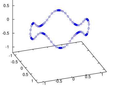
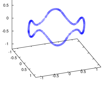
Figure 1. Illustration of importance of a suitable choice of the tangential redistribution. Left: no tangential redistribution. Right: tangential redistribution preserving the relative local length (i.e. $\omega=0$).

5. Existence and uniqueness of classical Hölder smooth solutions

In this section, we present results on the existence and uniqueness of the classical Hölder smooth solution to the system of equations (2) that governs the evolution of a curve $\Gamma$ parameterized by ${\mathbf{X}}$ and a scalar quantitity $\varrho$. We follow the analytical approach developed by Beneš, Kolář, Ševčovič [9]. The main idea of the proof is based on the abstract theory of analytic semiflows in Banach spaces due to DaPrato and Grisvard [10], Angenent [5, 4], Lunardi [29]. The proof of the local existence and uniqueness of a classical Hölder smooth solution is based on the analysis of the position vector equation (2) in which we choose the uniform tangential velocity $\alpha$. It leads to a uniformly parabolic equation (2) provided that the diffusion coefficient $a$ is uniformly bounded from below by a positive constant. In our proof method, the assumptions of strict positivity of the curvature $\kappa$ and the existence of the Frenet frame are not required. The main idea is to rewrite the system (2) in the form of an initial value problem for the abstract parabolic equation:

(12) $$\partial_{t}\Phi=\mathscr{F}(\Phi),\quad\Phi(0)=\Phi_{0},$$

in a scale of Banach spaces. Furthermore, we have to show that, for any $\tilde{\Phi}$, the linearization $\mathscr{A}=\mathscr{F}^{\prime}(\tilde{\Phi})$ generates an analytic semigroup and belongs to the so-called maximal regularity class. Since the source term $G$ may depend on the curvature $\kappa=|\partial_{s}{\mathbf{X}}\times\partial^{2}_{s}{\mathbf{X}}|=|\partial_{s}^{2}{\mathbf{X}}|$. Thus, the parabolic equation for $\varrho$ may depend on the derivative of highest order $|\partial_{s}^{2}{\mathbf{X}}|$. As a consequence, linearization $\mathscr{F}^{\prime}(\tilde{\Phi})$ is a skew symmetric linear operator having an off-diagonal term.

First, we define the underlying function spaces. Assume that $0<\varepsilon<1$ and $k$ is a non-negative integer. Let us denote by $h^{k+\varepsilon}(S^{1})$ the so-called little Hölder space, that is, the Banach space, which is the closure of $C^{\infty}$ smooth functions in the norm of the Banach space of $C^{k}$ smooth functions defined in the periodic domain $S^{1}$, and such that the $k$-th derivative is $\varepsilon$-Hölder smooth. The norm is given as a sum of the $C^{k}$ norm and the Hölder semi-norm of the $k$-th derivative. For a given $0<\varepsilon<1$ we define the following scale of Banach spaces of $\varepsilon$-Hölder continuous functions defined in the periodic domain $S^{1}$:

(13) $$E_{k}=h^{2k+\varepsilon}(S^{1})\times h^{2k+\varepsilon}(S^{1})\times h^{2k+\varepsilon}(S^{1}),\quad\mathscr{E}_{k}=E_{k}\times h^{2k+\varepsilon}(S^{1}),\quad k=0,1/2,1.$$

Recall the following continuous and compact embedding: ${\mathcal{E}}_{1}\hookrightarrow{\mathcal{E}}_{1/2}\hookrightarrow{\mathcal{E}}_{0}$. Furthermore, using the interpolation inequality at the scale of Hölder spaces we have

(14) $$\|\Phi\|_{{\mathcal{E}}_{\frac{1}{2}}}\leq\|\Phi\|_{{\mathcal{E}}_{1}}^{\frac{1}{2}}\|\Phi\|_{{\mathcal{E}}_{0}}^{\frac{1}{2}}\leq\delta\|\Phi\|_{{\mathcal{E}}_{1}}+\frac{1}{4\delta}\|\Phi\|_{{\mathcal{E}}_{0}},\quad\text{for any}\ \delta>0\ \text{and}\ \Phi\in{\mathcal{E}}_{1}.$$

For $a,b\in h^{1+\varepsilon}(S^{1})$ and ${\mathbf{t}}=(t_{1},t_{2},t_{3})^{T}\in E_{\frac{1}{2}}$ we define the matrix function

$$A(a,b,{\mathbf{t}})=aI+b[{\mathbf{t}}]_{\times}:=\left(\begin{array}[]{ccc}a&-bt_{3}&bt_{2}\\ bt_{3}&a&-bt_{1}\\ -bt_{2}&bt_{1}&a\end{array}\right).$$

Clearly, $a\partial^{2}_{s}{\mathbf{X}}+b(\partial_{s}{\mathbf{X}}\times\partial^{2}_{s}{\mathbf{X}})=A(a,b,\partial_{s}{\mathbf{X}})\partial^{2}_{s}{\mathbf{X}}$. Then the system of equations (2) can be rewritten as follows:

(15) $$\begin{split}\partial_{t}{\mathbf{X}}&=A(a,b,\partial_{s}{\mathbf{X}})\partial^{2}_{s}{\mathbf{X}}+{\mathbf{F}}({\mathbf{X}},\partial_{s}{\mathbf{X}},\varrho,\partial_{s}\varrho),\\ \partial_{t}\varrho&=c\partial^{2}_{s}\varrho+G({\mathbf{X}},\partial_{s}{\mathbf{X}},\varrho,\partial_{s}\varrho,\kappa).\end{split}$$

Let us denote $\Phi=({\mathbf{X}},\varrho)^{T}$. In what follows, we shall assume that the mappings

$${\mathcal{E}}_{1/2}\ni\Phi\mapsto F({\mathbf{X}},\partial_{s}{\mathbf{X}},\varrho,\partial_{s}\varrho)\in E_{0},$$

$${\mathcal{E}}_{1/2}\times h^{\varepsilon}(S^{1})\ni(\Phi,\kappa)\mapsto G({\mathbf{X}},\partial_{s}{\mathbf{X}},\varrho,\partial_{s}\varrho,\kappa)\in h^{\varepsilon}(S^{1}),$$

are $C^{1}$ continuous and globally Lipschitz continuous.

Then the system of governing equations (15) can be rewritten in the abstract form (12) where $\mathscr{F}$ is defined by the right-hand side of (15). Suppose that $\tilde{\Phi}=(\tilde{{\mathbf{X}}},\tilde{\varrho})^{T}\in\mathscr{E}_{1}$. Recall that $\kappa({\mathbf{X}})=|\partial_{s}{\mathbf{X}}\times\partial^{2}_{s}{\mathbf{X}}|=|A(0,1,\partial_{s}{\mathbf{X}})\partial^{2}_{s}{\mathbf{X}}|$. Therefore, the Fréchet derivative at $\tilde{{\mathbf{X}}}\in\mathscr{E}_{1}$ of $\kappa$ in the direction ${\mathbf{X}}\in\mathscr{E}_{1}$ has the form

$$\kappa^{\prime}(\tilde{{\mathbf{X}}}){\mathbf{X}}=\tilde{e}^{T}\left[A(0,1,\partial_{s}\tilde{{\mathbf{X}}})\partial^{2}_{s}{\mathbf{X}}+A(0,1,\partial_{s}{\mathbf{X}})\partial^{2}_{s}\tilde{{\mathbf{X}}}\right],\quad\text{where}\quad\tilde{e}=\frac{\partial_{s}\tilde{{\mathbf{X}}}\times\partial^{2}_{s}\tilde{{\mathbf{X}}}}{|\partial_{s}\tilde{{\mathbf{X}}}\times\partial^{2}_{s}\tilde{{\mathbf{X}}}|}\in E_{0}.$$

Hence the principal part $\mathscr{A}_{0}$ of the linearization $\mathscr{F}^{\prime}(\tilde{\Phi})$ containing the second-order derivatives has the matrix form $\partial_{t}\Phi=\mathscr{A}_{0}\Phi$ where $\mathscr{A}_{0}$ is a skew diagonal linear operator:

$$\mathscr{A}_{0}\Phi=\left(\begin{array}[]{cc}\tilde{A}&0\\ \tilde{d}^{T}&\tilde{c}\end{array}\right)\partial_{s}^{2}\Phi,$$

where $\tilde{a}=a(\tilde{{\mathbf{X}}},\partial_{s}\tilde{{\mathbf{X}}},\tilde{\varrho},\partial_{s}\tilde{\varrho})>0,\ \tilde{b}=b(\tilde{{\mathbf{X}}},\partial_{s}\tilde{{\mathbf{X}}},\tilde{\varrho},\partial_{s}\tilde{\varrho}),\ \tilde{c}=c(\tilde{{\mathbf{X}}},\partial_{s}\tilde{{\mathbf{X}}},\tilde{\varrho},\partial_{s}\tilde{\varrho})>0,\tilde{d}=G^{\prime}_{\kappa}(\tilde{{\mathbf{X}}},\partial_{s}\tilde{{\mathbf{X}}},\tilde{\varrho},\partial_{s}\tilde{\varrho},\tilde{\kappa})\tilde{e}^{T}A(0,1,\partial_{s}\tilde{{\mathbf{X}}})$, and $\tilde{A}=A(\tilde{a},\tilde{b},\partial_{s}\tilde{{\mathbf{X}}})$. Clearly, $\tilde{a},\tilde{b},\tilde{c},\tilde{A}_{ij}\in h^{1+\varepsilon}(S^{1}),\tilde{d}\in E_{\frac{1}{2}}$. The operator $\mathscr{A}_{0}$ generates an analytic semigroup $\{\exp(t\,\mathscr{A}_{0}),t\geq 0\}$ in $\mathscr{E}_{0}$,

$$\exp(t\,\mathscr{A}_{0})=\left(\begin{array}[]{cc}\exp(t\,\tilde{A}\partial^{2}_{s}),&0\\ D(t),&\exp(t\,\tilde{c}\partial^{2}_{s})\end{array}\right),$$

where $D(t)=\int_{0}^{t}\exp((t-\tau)\tilde{c}\partial^{2}_{s})(\tilde{d}^{T}\partial^{2}_{s})\exp(\tau\tilde{A}\partial^{2}_{s})d\tau$. Next, we will prove that $\mathscr{A}_{0}$ belongs to the maximal regularity class ${\mathcal{M}}(\mathscr{E}_{1},\mathscr{E}_{0})$. This means that for any time interval $[0,T],T>0$, the mapping $\partial_{t}-\mathscr{A}_{0}:\Phi\mapsto(\Phi_{0},f)$ from $C([0,T],\mathscr{E}_{1})\cap C^{1}([0,T],\mathscr{E}_{0})$ to $\mathscr{E}_{1}\times C([0,T],\mathscr{E}_{0})$, is invertible, where $f(t)=\partial_{t}\Phi(t)-\mathscr{A}_{0}\Phi(t),\ \Phi_{0}=\Phi(0)$, i.e., the inverse operator $(\partial_{t}-\mathscr{A}_{0})^{-1}:\mathscr{E}_{1}\times C([0,T],\mathscr{E}_{0})\to C([0,T],\mathscr{E}_{1})\cap C^{1}([0,T],\mathscr{E}_{0})$ exists and is a bounded linear operator. To prove this statement, assume $f=(f^{{\mathbf{X}}},f^{\varrho})\in C([0,T],\mathscr{E}_{0})=C([0,T],E_{0})\times C([0,T],h^{\varepsilon}(S^{1}))$, and $\Phi_{0}=({\mathbf{X}}_{0},\varrho_{0})\in\mathscr{E}_{1}=E_{1}\times h^{2+\varepsilon}(S^{1})$. Assume $\tilde{a},\tilde{b}\in h^{1+\varepsilon}(S^{1})$ and that the function $\tilde{a}$ is strictly positive, $T>0$. According to [9, Proposition 3] the operator $(\tilde{a}\pm i\tilde{b})\partial^{2}_{s}$ belongs to the maximal regularity class ${\mathcal{M}}(h^{2+\varepsilon}(S^{1}),h^{\varepsilon}(S^{1}))$ on the time interval $[0,T]$. Moreover, if $\tilde{{\mathbf{t}}}=\partial_{s}\tilde{{\mathbf{X}}}\in E_{\frac{1}{2}}$, then the linear operator $\tilde{A}\partial^{2}_{s}=A(\tilde{a},\tilde{b},\partial_{s}\tilde{{\mathbf{X}}})\partial^{2}_{s}$ belongs to the maximal regularity class ${\mathcal{M}}(E_{1},E_{0})$ in the time interval $[0,T]$. This means that the operator $\partial_{t}-\tilde{A}\partial^{2}_{s}:{\mathbf{X}}\ni C([0,T],E_{1})\cap C^{1}([0,T],E_{0})\mapsto({\mathbf{X}}_{0},f^{{\mathbf{X}}})\in E_{1}\times C([0,T],E_{0})$ is invertible. Similarly, the operator $\tilde{c}\partial^{2}_{s}$ belongs to the maximal regularity class ${\mathcal{M}}(h^{2+\varepsilon}(S^{1}),h^{\varepsilon}(S^{1}))$. Therefore, the inverse operator $(\partial_{t}-\mathscr{A}_{0})^{-1}$ is given by $\Phi=({\mathbf{X}},\varrho)=(\partial_{t}-\mathscr{A}_{0})^{-1}(\Phi_{0},f)$ is bounded. It can be expressed as ${\mathbf{X}}=(\partial_{t}-\tilde{A}\partial^{2}_{s})^{-1}({\mathbf{X}}_{0},f^{{\mathbf{X}}})$ and $\varrho=(\partial_{t}-\tilde{c}\partial^{2}_{s})^{-1}(\varrho_{0},\xi)$ where $\xi=f^{\varrho}+\tilde{d}^{T}\partial^{2}_{s}{\mathbf{X}}\in C([0,T],h^{\varepsilon}(S^{1}))$. As a consequence, $\mathscr{A}_{0}$ belongs to the maximal regularity class ${\mathcal{M}}(\mathscr{E}_{1},\mathscr{E}_{0})$.

We decompose the linearization $\mathscr{F}^{\prime}(\tilde{\Phi})=\mathscr{A}_{0}+\mathscr{A}_{1}$ where the operator $\mathscr{A}_{1}=\mathscr{F}^{\prime}(\tilde{\Phi})-\mathscr{A}_{0}$ contains lower first order derivatives $\partial^{k}_{s},k=0,1$, of $\tilde{\Phi}$. Furthermore, it is a bounded linear operator $\mathscr{A}_{1}:\mathscr{E}_{\frac{1}{2}}\to\mathscr{E}_{0}$. Therefore, the operator $\mathscr{A}_{1}$ considered as a mapping from $\mathscr{E}_{1}\to\mathscr{E}_{0}$ has the relative zero norm with respect to $\mathscr{A}_{0}$ . Therefore, the linearization $\mathscr{F}^{\prime}(\tilde{\Phi})$ belongs to the maximal regularity class ${\mathcal{M}}(\mathscr{E}_{1},\mathscr{E}_{0})$ because this class is closed with respect to perturbation with the relative zero norm (cf. [5, Lemma 2.5], DaPrato and Grisvard [10], Lunardi [29]). The method based on analytic semigroup and maximal regularity theory has been successfully applied to prove the existence, regularity and uniqueness of solutions representing evolving families of 2D and 3D curves in the series of papers co-authored by Ševčovič, Mikula, Yazaki, Beneš and Kolář [31], [32], [33], [42], [26], [8], [9].

Now, we can state the following result on the local existence and uniqueness of solutions.

Theorem 5.1.

Assume that the tangential velocity preserves the relative local length and is given by (10). Assume that the parameterization ${\mathbf{X}}_{0}={\mathbf{X}}(\cdot,0)$ of the initial curve $\Gamma_{0}$ belongs to the Hölder space ${\mathcal{E}}_{1}$, and the initial scalar quantity $\varrho=\varrho(\cdot,0)$ belongs to the space $h^{2+\varepsilon}(S^{1})$. Then there exist $T>0$ and a unique family of evolving curves $\{\Gamma_{t},t\in[0,T]\}$ evolving in 3D and the scalar quantity $\varrho$ to the system of nonlinear parabolic equations (2).

Proof.

The proof follows from the abstract result on the existence and uniqueness of solutions to (12) due to Angenent [5]. It is based on the linearization of the abstract evolution equation (12) in the Banach space $\mathscr{E}_{1}$. For any $\tilde{\Phi}$, the linearization $\mathscr{F}^{\prime}(\tilde{\Phi})$ generates an analytic semigroup and belongs to the maximal regularity class ${\mathcal{M}}(\mathscr{E}_{1},\mathscr{E}_{0})$ of linear operators from the Banach space $\mathcal{E}_{1}$ to the Banach space $\mathcal{E}_{0}$. The local existence and uniqueness of a solution $\Phi=({\mathbf{X}},\varrho)\in C([0,T],{\mathcal{E}}_{1})\cap C^{1}([0,T],{\mathcal{E}}_{0})$, and $\Phi(\cdot,0)=\Phi_{0}$ now follow from the abstract result [5, Theorem 2.7] due to Angenent.

∎

6. Semi-analytical examples of periodic solutions

In this section, we present two examples of the evolution of a circular curve with no torsion evolving in rotating and parallel planes. The motion of the curves is coupled by a scalar quantity $\varrho$. The method of construction of a solution in a special separated form and its reduction to solving a system of ODEs has been proposed in the recent paper by Beneš, Kolář and Ševčovič in the context of evolving 3D curves with interactions [9]. We consider the following system of coupled equations governing the motion of curves in 3D and scalar quantity:

(16) $$\begin{split}&\partial_{t}{\mathbf{X}}=\beta{\mathbf{N}}+\gamma{\mathbf{B}},\\ &\partial_{t}\varrho-\kappa\beta\varrho=\partial_{s}^{2}\varrho+q.\end{split}$$

The normal velocity $\beta$, the binormal velocity and $\gamma$, and the source term $q$ are assumed to depend on the shape of the curve $\Gamma_{t}=\{{\mathbf{X}}(u,t),u\in I\}$ and the scalar quantity $\varrho$. In this example, we shall assume a specific choice:

(17) $$\beta=\kappa-\frac{2\pi}{L(\Gamma)}-\tilde{P}(L(\Gamma),\|\varrho\|_{2}),\quad q=\frac{\varrho}{\sqrt{2}\|\varrho\|_{2}},$$

where $\tilde{P}$ is a smooth function, and $\|\varrho\|_{2}=\left(\int_{0}^{1}\varrho(u)^{2}du\right)^{\frac{1}{2}}$ is the $L^{2}$-norm of $\varrho$.

If the family $\Gamma_{t},t\geq 0,$ of curves evolves in parallel planes, then the area $A(\Gamma)$ enclosed by the curve $\Gamma$ satisfies $\frac{d}{dt}A(\Gamma)=-\int_{\Gamma}\beta ds$ (see [9, Prop. 2]). Since $\int_{\Gamma}\kappa ds=2\pi$ for a curve evolving in the plane, we have $\int_{\Gamma}\beta ds=0$ provided that $\beta=\kappa-\frac{2\pi}{L(\Gamma)}$ (see Gage [16]). In such a case, the enclosed area $A(\Gamma)$ is preserved during evolution. In the next two examples, we will show that a perturbation of the normal velocity $\beta=\kappa-\frac{2\pi}{L(\Gamma)}$ and consideration of the influence of the scalar quantity $\varrho$ may lead to periodic motion of the curves and the scalar quantity.

6.1. An example of coupled system of parabolic equations for evolution of a curve and scalar quantity illustrating a supercritical Hopf bifurcation

In the first example, we construct the solution ${\mathbf{X}}$ in the form of circular curves with radius $r$ evolving in a rotating plane. Define the vectors $\hat{{\mathbf{X}}}(u)=(\cos 2\pi u,\sin 2\pi u,0)^{T}$ and $\hat{{\mathbf{X}}}^{\perp}(u)=(-\sin 2\pi u,\cos 2\pi u,0)^{T}$. Assume that a $3\times 3$ orthogonal matrix $Q$ and a positive scalar $r>0$ are time-dependent functions. Let the family of evolving curves $\Gamma_{t}=\{{\mathbf{X}}(u,t),u\in I,t\geq 0\}$ be defined as follows:

(18) $${\mathbf{X}}(u,t)=r(t)Q(t)\hat{{\mathbf{X}}}(u).$$

Then, for the curvature $\kappa$, arc-lenth parametrization $s$, tangent ${\mathbf{T}}$, normal ${\mathbf{N}}$ and binormal ${\mathbf{B}}$ vectors we have

$$\kappa=|\partial_{s}^{2}{\mathbf{X}}|=1/r,\quad ds=2\pi r\,du,\quad{\mathbf{T}}=Q\hat{{\mathbf{X}}}^{\perp},\quad{\mathbf{N}}=-Q\hat{{\mathbf{X}}},\quad{\mathbf{B}}=Qe_{3},\quad e_{3}=(0,0,1)^{T}.$$

Assume that the function $\omega(t)$ satisfies $r(t)\frac{d\omega}{dt}(t)=1$. Then, it is easy to verify that if

$$Q(t)=\begin{pmatrix}\cos\omega(t)&0&-\sin\omega(t)\\ 0&1&0\\ \sin\omega(t)&0&\cos\omega(t)\\ \end{pmatrix}\ \ \text{then}\ \ QQ^{T}=Q^{T}Q=I,\ \ r\frac{d}{dt}Q=Q\begin{pmatrix}0&0&-1\\ 0&0&0\\ 1&0&0\\ \end{pmatrix}.$$

Therefore $\partial_{t}{\mathbf{X}}=\frac{d}{dt}(rQ)\hat{{\mathbf{X}}}=\frac{dr}{dt}Q\hat{{\mathbf{X}}}+r\frac{d}{dt}Q\hat{{\mathbf{X}}}=-\frac{dr}{dt}{\mathbf{N}}+\gamma Qe_{3}=\beta{\mathbf{N}}+\gamma{\mathbf{B}}$ where $\gamma=\cos 2\pi u$ and $\beta=-\frac{dr}{dt}$. We search for the solution $\varrho$ in separated form:

(19) $$\varrho(u,t)=a(t)\cos 2\pi u,$$

where $a=a(t)\geq 0$ is a nonnegative amplitude. As $\|\varrho(\cdot,t)\|_{2}=\left(\int_{0}^{1}a(t)^{2}(\cos 2\pi u)^{2}du\right)^{\frac{1}{2}}=\frac{a(t)}{\sqrt{2}}$ we have $\gamma=q=\frac{\varrho}{\sqrt{2}\|\varrho\|_{2}}=\cos 2\pi u$. Therefore, for the normal velocity $\beta$ given by (17) we have $\beta=1/r-2\pi/(2\pi r)-\tilde{P}(\Gamma,\varrho)=-P(r,a)$, where $P(r,a)=\tilde{P}(L(\Gamma),\|\varrho\|_{2})$. Since $ds=2\pi rdu$ we have $\partial_{s}^{2}\varrho=(2\pi r)^{2}\partial_{u}^{2}\varrho=-ar^{-2}\cos 2\pi u$. Therefore,

$$\partial_{t}\varrho-\kappa\beta\varrho-\partial_{s}^{2}\varrho=\left(\frac{d}{dt}a+\frac{a}{r}P(r,a)+\frac{a}{r^{2}}\right)\cos 2\pi u.$$

As a consequence, the pair $({\mathbf{X}},\varrho)$ is a solution to the coupled evolutionary equation (16) if and only if the radius $r$ and the amplitude $a$ satisfy the planar ODE system:

(20) $$\frac{d}{dt}r=P(r,a),\qquad\frac{d}{dt}a=-\frac{a}{r}P(r,a)-\frac{a}{r^{2}}+1.$$

System (20) of ODEs has a nontrivial steady state $(\tilde{r},\tilde{a})$, i.e. the time-independent solution, where

$$\tilde{a}=\tilde{r}^{2},\qquad P(\tilde{r},\tilde{r}^{2})=0.$$

The linearization $\mathcal{A}$ of the right-hand side of (20) at the steady state $(\tilde{r},\tilde{a})$ has the form of a $2\times 2$ matrix $\mathcal{M}$:

$$\mathcal{A}=\begin{pmatrix}\frac{\partial P}{\partial r}(\tilde{r},\tilde{a})&\frac{\partial P}{\partial a}(\tilde{r},\tilde{a})&\\ \\ -\frac{\tilde{a}}{\tilde{r}}\frac{\partial P}{\partial r}(\tilde{r},\tilde{a})+2\frac{\tilde{a}}{\tilde{r}^{3}}&-\frac{\tilde{a}}{\tilde{r}}\frac{\partial P}{\partial a}(\tilde{r},\tilde{a})-\frac{1}{\tilde{r}^{2}}\end{pmatrix}.$$

Now, as $\tilde{a}=\tilde{r}^{2}$ we have

$$trace(\mathcal{A})=\frac{\partial P}{\partial r}(\tilde{r},\tilde{a})-\tilde{r}\frac{\partial P}{\partial a}(\tilde{r},\tilde{a})-\frac{1}{\tilde{r}^{2}},\qquad det(\mathcal{A})=-\frac{1}{\tilde{r}^{2}}\left(\frac{\partial P}{\partial r}(\tilde{r},\tilde{a})+2\tilde{r}\frac{\partial P}{\partial a}(\tilde{r},\tilde{a})\right).$$

Assume that the source term $\tilde{P}$ has the specific form

$$\tilde{P}(L(\Gamma),\|\varrho\|_{2})=\frac{L^{2}}{4\pi^{2}}-\lambda\sqrt{2}\|\varrho\|_{2}+1,\quad\text{that is},\quad P(a,r)=r^{2}-\lambda a+1,$$

where $\lambda>1$ is a parameter. Then, for the steady-state solution $(\tilde{r},\tilde{a})$ we have $\tilde{r}=1/\sqrt{\lambda-1},\tilde{a}=1/(\lambda-1)$.

$$trace(\mathcal{A})=\frac{\lambda+2}{\sqrt{\lambda-1}}-\lambda+1,\qquad det(\mathcal{A})=(\lambda-1)^{3/2}.$$

The nonlinear equation $trace(\mathcal{A})=0$ has the unique solution for the parameter value $\lambda_{0}=4.473402$. Since $trace(\mathcal{A})<0$ for $\lambda>\lambda_{0}$, and $trace(\mathcal{A})>0$ for $\lambda<\lambda_{0}$. Hence, the supercritical Hopf bifurcation occurs when the parameter $\lambda$ crosses the critical value $\lambda_{0}$. From a stable focus steady state $(\tilde{r},\tilde{a})$ for $\lambda>\lambda_{0}$ we observe a bifurcation to a stable period orbit at $\lambda_{0}$ that persists to exist for $\lambda<\lambda_{0}$.

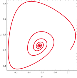
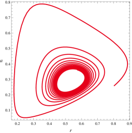
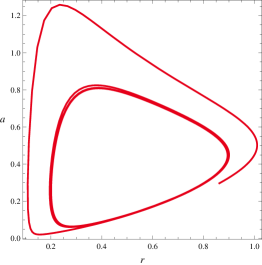
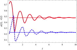
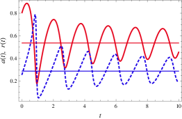
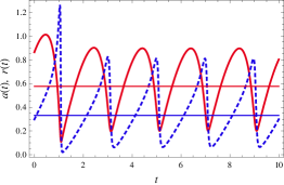
Figure 2. Top row: phase portraits of solutions of (2). Bottom row: time dependent trajectories of solutions for the parameter values $\lambda=5.36808$ (left), $\lambda=\lambda_{0}=4.473402$ (middle), and $\lambda=4.02606$ (right).

6.2. Another example of a coupled system of parabolic equations for evolution of a curve and scalar quantity

In this example, we will construct a family of curves evolving in parallel planes and scalar quantity $\varrho$ such that it solves the coupled system of evolution equations (16) with binormal velocity $\gamma=-\beta$. Assume that the family of circular curves $\Gamma_{t}=\{{\mathbf{X}}(u,t),u\in[0,1]\}$ evolves in parallel planes and is parameterized by

$${\mathbf{X}}(u,t)=(r(t)\cos 2\pi u,r(t)\sin 2\pi u,r(t))^{T},\qquad\varrho(u,t)=a(t)\cos 2\pi u.$$

Similarly to the previous example, we consider the normal velocity $\beta$ and the external source term $q$ of the form (17). Since ${\mathbf{N}}=-(\cos 2\pi u,\sin 2\pi u,0)^{T}$ and ${\mathbf{B}}=(0,0,1)^{T}$ it is easy to verify that $({\mathbf{X}},\varrho)$ is a solution to (16) with binormal velocity $\gamma=-\beta$ if and only if $\frac{d}{dt}r=-\beta$ and amplitude $a$ satisfies the ODE: $\frac{d}{dt}a-\frac{a}{r}\beta+\frac{a}{r^{2}}=1$. Therefore, for the normal velocity $\beta$ given by (17) we have $\beta=1/r-2\pi/(2\pi r)-\tilde{P}(\Gamma,\varrho)=-P(r,a)$, where $P(r,a)=\tilde{P}(\Gamma,\|\varrho\|_{2})=r^{2}-\lambda a+1$. It means that the pair of functions $(r,\varrho)$ satisfies the system of ODEs (20) that exhibits a Hopf supercritival bifurcation at the parametrix value $\lambda=4.02606<\lambda_{0}=4.473402$. In Fig. 3 we present an example of the evolution of concentric circles with radius $r$ converging to $\tilde{r}=1/\sqrt{\lambda-1}$ and the amplitude of the scalar quantity $a$ converging to $\tilde{a}=1/(\lambda-1)$ for the parameter value $\lambda=5.36808>\lambda_{0}$.

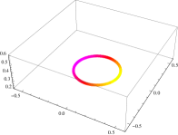
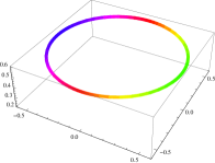
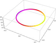
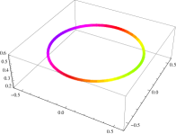
$t=0.8$                                      $t=1.8$                                      $t=4$                                      $t=8$

Figure 3. Evolution of circular curves $\Gamma_{t}$ and the scalar quantity $\varrho(\cdot,t)$ (displayed as a colored field) that solve the coupled system (17) with the parameter value $\lambda=5.36808>\lambda_{0}$.

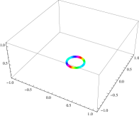
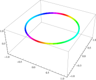
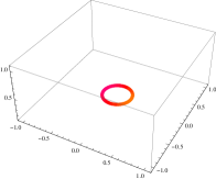
$t=2.5$                                      $t=3.1$                                      $t=4.4$                                      $t=5.2$

Figure 4. Evolution of circular curves $\Gamma_{t}$ and the scalar quantity $\varrho(\cdot,t)$ (displayed as a coloured field)that solve the coupled system (17) with the parameter value $\lambda=4.02606<\lambda_{0}$.

7. Numerical discretization scheme based on the method of flowing finite volumes and the method of lines

In this section, we present a numerical discretization scheme to solve the system of equations (2). Our full space-time discretization scheme is based on a combination of the method of lines and the flowing finite-volume method of spatial discretization. The flowing finite-volume discretization was proposed by Mikula and Ševčovič [31] for the evolution of curves in the plane. It was further generalized and analyzed for evolving curves in 3D by Beneš, Kolář and Ševčovič in [8, 9].

7.1. Method of flowing finite volumes

In this section, we describe the discretization method in more detail. We consider $M$ discrete nodes ${\mathbf{X}}_{k}$ approximating points ${\mathbf{X}}(u_{k})$, $k=0,1,\ldots,M$, along the curve $\Gamma=\{{\mathbf{X}}(u),u\in I\}$, $u_{k}=k/M$. Similarly, we approximate the values of the scalar quantity $\varrho_{k}=\varrho(u_{k})$. The corresponding dual nodes are defined as ${\mathbf{X}}_{k\pm\frac{1}{2}}={\mathbf{X}}(u_{k\pm\frac{1}{2}})$ (see Fig. 5). Here, $u_{k\pm\frac{1}{2}}=u_{k}\pm\frac{h}{2}$, where $h=1/M$, and $({\mathbf{X}}_{k}+{\mathbf{X}}_{k+1})/2$ denote averages on segments connecting discrete nodes in the vicinity. It may differ from the position ${\mathbf{X}}_{k+\frac{1}{2}}\in\Gamma$. The $k$-th segment between ${\mathbf{X}}_{k-1}$ and ${\mathbf{X}}_{k}$ represents the finite volume, while the segment between ${\mathbf{X}}_{k-1/2}$ and ${\mathbf{X}}_{k+1/2}$ represents the dual finite volume. Integration of equations (2) for $({\mathbf{X}},\varrho)$ in the dual volume between the dual nodes ${\mathbf{X}}_{k-\frac{1}{2}}$ and ${\mathbf{X}}_{k+\frac{1}{2}}$ yields the following result:

(21) $$\begin{split}&\int_{u_{k-\frac{1}{2}}}^{u_{k+\frac{1}{2}}}\partial_{t}{\mathbf{X}}|\partial_{u}{\mathbf{X}}|du=\int_{u_{k-\frac{1}{2}}}^{u_{k+\frac{1}{2}}}a\frac{\partial}{\partial u}\left(\frac{\partial_{u}{\mathbf{X}}}{|\partial_{u}{\mathbf{X}}|}\right)+b(\partial_{s}{\mathbf{X}}\times\partial_{s}^{2}{\mathbf{X}})|\partial_{u}{\mathbf{X}}|+{\mathbf{F}}|\partial_{u}{\mathbf{X}}|\ du,\\ &\int_{u_{k-\frac{1}{2}}}^{u_{k+\frac{1}{2}}}\partial_{t}\varrho|\partial_{u}{\mathbf{X}}|du=\int_{u_{k-\frac{1}{2}}}^{u_{k+\frac{1}{2}}}c\frac{\partial}{\partial u}\left(\frac{\partial_{u}\varrho}{|\partial_{u}{\mathbf{X}}|}\right)+G|\partial_{u}{\mathbf{X}}|\ du.\end{split}$$

We denote $d_{k}=|{\mathbf{X}}_{k}-{\mathbf{X}}_{k-1}|$, $d_{M+1}=d_{1}$, and $d_{k+\frac{1}{2}}=(d_{k+1}+d_{k})/2$ for $k=0,1,\ldots,M$, where ${\mathbf{X}}_{0}={\mathbf{X}}_{M}$ and ${\mathbf{X}}_{1}={\mathbf{X}}_{M+1}$ for a closed curve $\Gamma$. We approximate the integral terms in (21) using the flowing finite-volume method. We assume that the quantities $\partial_{t}{\mathbf{X}},\partial_{u}{\mathbf{X}},{\mathbf{F}},\partial_{t}\varrho,\partial_{u}\varrho$ and $G$ are constant in the finite volume between the nodes ${\mathbf{X}}_{k+\frac{1}{2}}$ and ${\mathbf{X}}_{k-\frac{1}{2}}$, and taking the values $\partial_{t}{\mathbf{X}}_{k},\partial_{u}{\mathbf{X}}_{k},{\mathbf{F}}_{k},\partial_{t}\varrho_{k},\partial_{u}\varrho_{k}$, and $G_{k}$ an respectively. Then the approximation of the terms of the first equation in (21) reads as follows:

(22) $$\begin{split}&\int_{u_{k-\frac{1}{2}}}^{u_{k+\frac{1}{2}}}\partial_{t}{\mathbf{X}}|\partial_{u}{\mathbf{X}}|du\approx\frac{d{\mathbf{X}}_{k}}{dt}d_{k+\frac{1}{2}},\\ &\int_{u_{k-\frac{1}{2}}}^{u_{k+\frac{1}{2}}}a\partial_{u}\left(\frac{\partial_{u}{\mathbf{X}}}{|\partial_{u}{\mathbf{X}}|}\right)du\approx a_{k}\left(\frac{{\mathbf{X}}_{k+1}-{\mathbf{X}}_{k}}{d_{k+1}}-\frac{{\mathbf{X}}_{k}-{\mathbf{X}}_{k-1}}{d_{k}}\right),\\ &\int_{u_{k-\frac{1}{2}}}^{u_{k+\frac{1}{2}}}b(\partial_{s}{\mathbf{X}}\times\partial_{s}^{2}{\mathbf{X}})|\partial_{u}{\mathbf{X}}|du\approx b_{k}d_{k+\frac{1}{2}}\kappa_{k}{\mathbf{B}}_{k},\ \ \int_{u_{k-\frac{1}{2}}}^{u_{k+\frac{1}{2}}}{\mathbf{F}}|\partial_{u}{\mathbf{X}}|du\approx{\mathbf{F}}_{k}d_{k+\frac{1}{2}}.\end{split}$$

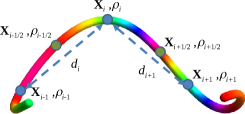
Figure 5. Discretization of a segment of a 3D curve by the method of flowing finite volumes.

Analogously, we can approximate the terms entered into the second equation in (21) for the scalar quantity $\varrho$. Approximations of the nonnegative curvature $\kappa=|\partial^{2}_{s}{\mathbf{X}}|$, tangent vector ${\mathbf{T}}=\partial_{s}{\mathbf{X}}$, normal vector ${\mathbf{N}}=\partial^{2}_{s}{\mathbf{X}}/|\partial^{2}_{s}{\mathbf{X}}|$ and binormal vector ${\mathbf{B}}={\mathbf{T}}\times{\mathbf{N}}$ read as follows:

(23) $$\begin{split}&\kappa_{k}\approx\left|\frac{2}{d_{k}+d_{k+1}}\left(\frac{{\mathbf{X}}_{k+1}-{\mathbf{X}}_{k}}{d_{k+1}}-\frac{{\mathbf{X}}_{k}-{\mathbf{X}}_{k-1}}{d_{k}}\right)\right|,\ {\mathbf{T}}_{k}\approx\frac{{\mathbf{X}}_{k+1}-{\mathbf{X}}_{k-1}}{d_{k+1}+d_{k}},\\ &{\mathbf{N}}_{k}\approx\left(\frac{{\mathbf{X}}_{k+1}-{\mathbf{X}}_{k}}{d_{k+1}}-\frac{{\mathbf{X}}_{k}-{\mathbf{X}}_{k-1}}{d_{k}}\right)\big{/}\left|\frac{{\mathbf{X}}_{k+1}-{\mathbf{X}}_{k}}{d_{k+1}}-\frac{{\mathbf{X}}_{k}-{\mathbf{X}}_{k-1}}{d_{k}}\right|.\end{split}$$

In approximation ${\mathbf{F}}_{k}$ of the vector-valued function ${\mathbf{F}}$, we assume that the curve $\Gamma$ entering the definition of ${\mathbf{F}}$ is approximated by a polygonal curve with vertices $({\mathbf{X}}_{0},{\mathbf{X}}_{1},\ldots,{\mathbf{X}}_{M})$. The semi-discrete scheme for solving (2) can be written as follows:

(24) $$\begin{split}\frac{d{\mathbf{X}}_{k}}{dt}&=a_{k}\frac{1}{d_{k+\frac{1}{2}}}\left(\frac{{\mathbf{X}}_{k+1}-{\mathbf{X}}_{k}}{d_{k+1}}-\frac{{\mathbf{X}}_{k}-{\mathbf{X}}_{k-1}}{d_{k}}\right)+b_{k}\kappa_{k}{\mathbf{B}}_{k}+{\mathbf{F}}_{k},\\ \frac{d\varrho_{k}}{dt}&=a_{k}\frac{1}{d_{k+\frac{1}{2}}}\left(\frac{\varrho_{k+1}-\varrho_{k}}{d_{k+1}}-\frac{\varrho_{k}-\varrho_{k-1}}{d_{k}}\right)+G_{k},\\ {\mathbf{X}}_{k}(0)&={\mathbf{X}}_{ini}(u_{k}),\quad\varrho_{k}(0)=\varrho_{ini}(u_{k}),\quad\text{for}\ k=1,\ldots,M.\end{split}$$

Resulting system (24) of ODEs is solved numerically by means of the 4th-order explicit Runge-Kutta-Merson scheme with automatic time stepping control and the tolerance parameter $10^{-3}$ (see [37]). We chose the initial time step as $4h^{2}$, where $h=1/M$ is the spatial mesh size.

7.2. Experimental order of convergence

We test the numerical scheme proposed in Section 7.1 on a simple example in which we choose $\beta=\kappa,\gamma=0,{\mathbf{F}}=0$ and $G=-\partial_{s}(v\varrho)+\varrho^{3}+g$,

(25) $$\begin{split}&\partial_{t}{\mathbf{X}}=\partial^{2}_{s}{\mathbf{X}},\\ &\partial_{t}\varrho-\kappa^{2}\varrho=\partial_{s}^{2}\varrho-\partial_{s}(v\varrho)+\varrho^{3}+g,\end{split}$$

where $v=-10$ and the function $g(u,t)$ is chosen such that the prescribed function $\varrho(u,t)=\cos(t)(\sin(2\pi u)+\sin(4\pi u))$ is the analytical solution of (25) satisfying the initial condition ${\mathbf{X}}(u,0)=(\cos 2\pi u,\sin 2\pi u,0)^{T},\varrho(u,0)=\sin(2\pi u)+\sin(4\pi u)$. Here $t\in[0,T]$ where $T=45$. Assuming that error estimates $err(M)=const(1/M)^{EOC}$ depend on the number of finite volumes $M$, the value of the experimental order of convergence (EOC) between two levels of meshes containing $M_{1}$ and $M_{2}$ finite volumes is given by

$$EOC=\frac{\log(err(M_{1})/err(M_{2}))}{\log(M_{2}/M_{1})}.$$

The computational results are summarized in Table 1. They indicate the second order of convergence of the proposed numerical scheme.

Table 1. The experimental order of convergence for errors measured in the discrete $L^{1}$ and $L^{\infty}$ norms.

	$L^{1}((0,T);L^{\infty}(S^{1}))$		$L^{\infty}((0,T);L^{\infty}(S^{1}))$
$M$	error norm	EOC	error norm	EOC
100	1.2975$\cdot 10^{-3}$	–	2.8703$\cdot 10^{-3}$	–
200	3.3382$\cdot 10^{-4}$	1.9586	7.4222$\cdot 10^{-4}$	1.9513
300	1.5312$\cdot 10^{-4}$	1.9222	3.4151$\cdot 10^{-4}$	1.9145
400	8.9079$\cdot 10^{-5}$	1.8830	1.9907$\cdot 10^{-4}$	1.8760
500	5.9055$\cdot 10^{-5}$	1.8421	1.3213$\cdot 10^{-4}$	1.8368

8. Numerical examples

In this section we present two examples of the evolution of closed curves in 3D. In the first example, we consider a simple curve without knots. On the other hand, in the second example we investigate the evolution of initial knotted curves.

8.1. An example of an evolution of 3D simple unknotted curves and scalar quantity

In the first numerical example, we consider a system of governing equations where the normal and binormal velocities and the external source term are given by $\beta=\kappa,\gamma=0$ and ${\mathbf{F}}=0$. Since $\beta{\mathbf{N}}=\kappa{\mathbf{N}}=\partial^{2}_{s}{\mathbf{X}}$, i.e.

(26) $$\begin{split}&\partial_{t}{\mathbf{X}}=\partial^{2}_{s}{\mathbf{X}},\\ &\partial_{t}\varrho-\kappa^{2}\varrho=\partial_{s}^{2}\varrho.\end{split}$$

A solution $({\mathbf{X}},\varrho)$ is subject to the initial condition ${\mathbf{X}}(u,0)=(\cos 2\pi u,\sin 2\pi,\sin 8\pi u)^{T}$, $\varrho(u,0)=1$ if $u\in(1/4,3/4)$ and $\varrho(u,0)=0$, otherwise. The evolution of the simple unknotted curve is depicted in Fig. 6. The values of the scalar quantity $\varrho$ are displayed by the color function. In the subsequent figures shown in Fig. 6 we depict the evolution of the initial curve approaching the shrinking circle for time levels $t\in\{0.062,0.124,0.19,0.25\}$.

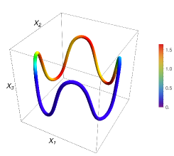
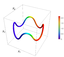
$t=0.062$                                                                  $t=0.124$

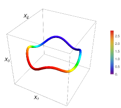
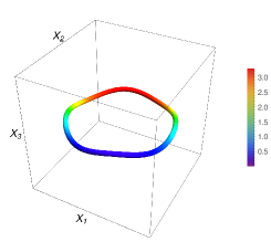
$t=0.19$                                                                  $t=0.25$

Figure 6. Numerical solution of problem (8) with advection velocity $v=20$ and $F=0$. Evolving curves approach the planar curve shortening the flow shrinking to a point in finite time.

8.2. An example of evolution of knotted curves and scalar quantity

A Fourier knot is a closed curve in 3D that can be parameterized by a finite Fourier series in the parameter $u\in[0,1]$. As an example, we consider a figure-eight knot (also called Listing’s knot) which can be parameterized by the following finite trigonometric series:

(27) $${\mathbf{X}}(u,0)=(\cos(4\pi u),\ \sin(6\pi u+1/2),\ (\cos(10\pi u+1/2)+\sin(6\pi u+1/2))/2)^{T},$$

$u\in[0,1]$. Its top view shape is shown in Fig. 7 (left).

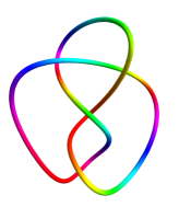
Figure 7. Left: The initial Fourier knotted curve (left). Right: The arrows placed on the curve represent the Biot-Savart vector field ${\mathbf{F}}({\mathbf{X}},\Gamma),{\mathbf{X}}\in\Gamma$ given by (28).

As an example of a nonlocal source term ${\mathbf{F}}={\mathbf{F}}_{0}$ we assume the external force corresponding to the Biot-Savart law. It represents the integrated influence of all points ${\mathbf{X}}$ that belong to the curve $\Gamma=\{{\mathbf{X}}(s),s\in[0,L(\Gamma)]\}$ at a given point ${\mathbf{X}}\in\mathbb{R}^{3}$.

(28) $${\mathbf{F}}({\mathbf{X}},\Gamma)=\int_{\Gamma}\frac{({\mathbf{X}}-{\mathbf{X}}(s))\times{\mathbf{T}}(s)}{|{\mathbf{X}}-{\mathbf{X}}(s)|_{\delta}^{3}}ds.$$

Following [9] we replaced the Euclidean distance between points ${\mathbf{X}}$ and ${\mathbf{X}}(s)$ by its regularization $|{\mathbf{X}}-{\mathbf{X}}(s)|_{\delta}=(\delta^{2}+|{\mathbf{X}}-{\mathbf{X}}(s)|^{2})^{\frac{1}{2}}$ where $0<\delta\ll 1$ is a small regularization parameter. The vector field ${\mathbf{F}}$ corresponding to the regularized Biot-Savart force (28) is shown in Fig. 7 (right).

Remark 1.

Assume that the torsion $\tau$ of a curve $\Gamma$ is equal to zero. Then the curve $\Gamma$ belongs to a plane. Let ${\mathbf{X}}\in\Gamma$. If ${\mathbf{N}}$ and ${\mathbf{T}}$ are the unit normal and tangent vectors at ${\mathbf{X}}$, then the Biot-Savart force projected onto the normal and tangent vectors vanishes, that is, ${\mathbf{F}}({\mathbf{X}},\Gamma)\cdot{\mathbf{N}}={\mathbf{F}}({\mathbf{X}},\Gamma)\cdot{\mathbf{T}}=0$. In fact, if $\Gamma$ belongs to a plane, then the difference of the position vectors ${\mathbf{X}}-{\mathbf{X}}(s)$, the tangent vector ${\mathbf{T}}(s)$ in ${\mathbf{X}}(s)$ as well as the vectors ${\mathbf{N}},{\mathbf{T}}$ belong to the same plane, and so $(({\mathbf{X}}-{\mathbf{X}}(s))\times{\mathbf{T}}(s))\cdot{\mathbf{N}}=(({\mathbf{X}}-{\mathbf{X}}(s))\times{\mathbf{T}}(s))\cdot{\mathbf{T}}=0$ for each $s\in[0,L(\Gamma)]$.

For example, if the curve $\Gamma$ is a circle parameterized by ${\mathbf{X}}(s)=(\cos s,\sin s,0)^{T},s\in[0,2\pi]$, then it is easy to verify that ${\mathbf{F}}({\mathbf{X}},\Gamma)\cdot{\mathbf{B}}=\int_{0}^{2\pi}(1-\cos s)(\delta^{2}+2(1-\cos s))^{-\frac{3}{2}}$. Notice that ${\mathbf{F}}({\mathbf{X}},\Gamma)\cdot{\mathbf{B}}=\infty$ if $\delta=0$.

Remark 2.

If $\Gamma$ and $\tilde{\Gamma}$ are two non-intersecting curves in 3D then the Gauss linking integral of $\Gamma$ and $\tilde{\Gamma}$ can be defined as follows:

$$link(\Gamma,\tilde{\Gamma}) = \frac{1}{4\pi}\oint_{\Gamma}\oint_{\tilde{\Gamma}}\frac{det\left(\partial_{s}{\mathbf{X}}(s),\partial_{\tilde{s}}\tilde{{\mathbf{X}}}({\tilde{s}}),{\mathbf{X}}(s)-\tilde{{\mathbf{X}}}({\tilde{s}})\right)}{|{\mathbf{X}}(s)-{\mathbf{X}}(\tilde{s})|^{3}}dsd\tilde{s}$$

$$= -\frac{1}{4\pi}\oint_{\Gamma}{\mathbf{F}_{0}}({\mathbf{X}}(s),\tilde{\Gamma})\cdot\partial_{s}{\mathbf{X}}(s)ds$$

where $\Gamma$ and $\tilde{\Gamma}$ are parameterized by ${\mathbf{X}}(s)$ and $\tilde{{\mathbf{X}}}$, respectively. The linking number $link(\Gamma,\tilde{\Gamma})$ computes the total signed area of the image of the Gauss map divided by the area $4\pi$ of the unit sphere in 3D.

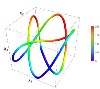
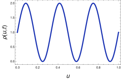
Figure 8. The initial knotted Fourier curve ${\mathbf{X}}=(X_{1},X_{2},X_{3})^{T}$ and the initial scalar quantity $\varrho(u,0)=1+\sin(6\pi u)$.

We consider the system of governing equation of the form:

(29) $$\begin{split}&\partial_{t}{\mathbf{X}}=\beta{\mathbf{N}}+\gamma{\mathbf{B}}+{\mathbf{F}}({\mathbf{X}},\Gamma),\\ &\partial_{t}\varrho-\kappa\beta\varrho=\partial_{s}^{2}\varrho.\end{split}$$

where $\beta=\kappa-\frac{2\pi}{L(\Gamma)}$. As an initial condition for the system (29) we consider the Fourier knotted curve shown in Fig. 8 and the initial scalar quantity $\varrho(u,0)=1+\sin(6\pi u)$.

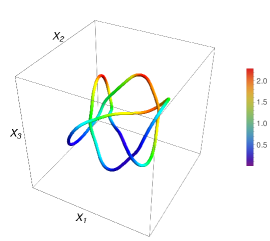
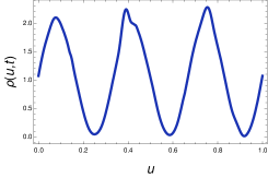
$t=0.02$

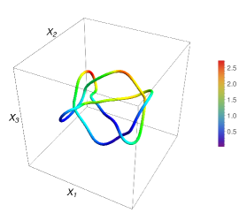
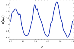
$t=0.063$

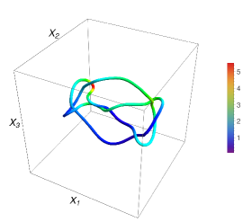
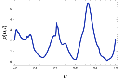
$t=0.124$

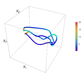
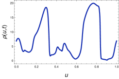
$t=0.237$

Figure 9. Evolution of the initial knotted curve shown in Fig. 8 with the velocity $\gamma=\varrho$ and the external force given by the regularized Biot-Savart force given by (28).

In the first experiment shown in Fig. 9 we investigate the motion of the initial knotted curve (8) with the binormal velocity $\gamma=\varrho$ linearly depending on the scalar quantity $\varrho$. The external force given by the regularized Biot-Savart force (28). The presence of the Biot-Savart force ${\mathbf{F}}$ ensures that the evolved curves preserve the topological structure of a knotted curve.

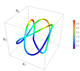
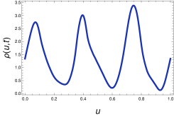
$t=0.1225$

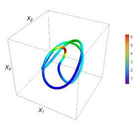
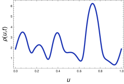
$t=0.25$

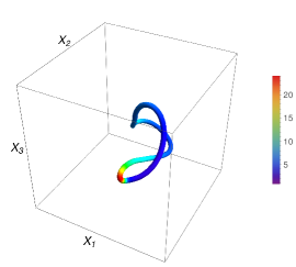
$t=0.4$

Figure 10. Evolution of the initial knotted curve with the binormal velocity $\gamma=\varrho$ and the vanishing force ${\mathbf{F}}=0$.

The third experiment is shown in Fig. 10. The same initial knotted curve in Fig. 8 is evolved by the binormal velocity $\gamma=\varrho$ and vanishing external force ${\mathbf{F}}=0$. In contrast to the experiments shown in Fig. 9 the knotted structure is not preserved and the evolved curve approaches a circular curve in the plane.

9. Conclusions

In this paper, we investigated the motion of closed smooth curves that evolve in $\mathbb{R}^{3}$ coupled with the evolution of a scalar quantity evaluated over the evolving curve. We proved the local existence and uniqueness oflassical Hölder smooth solutions. The proof is based on the analysis of the position vector equation and the parabolic equation for the evolving scalar quantity. We also proposed a numerical discretization scheme for numerical approximation of the evolving family of curves and scalar quantity. We presented several numerical examples of evolving curves and the scalar quantity.

Acknowledgments. The first and second authors received partial support from the project 21-09093S of the Czech Science Foundation. The third author received support from the Slovak Research and Development Agency under the project APVV-20-0311.

References

- [1]
- [2] S. J. Altschuler, Singularities of the curve shrinking flow for space curves, J. Differ. Geom., 34 (1991), pp. 491-514.
- [3] S. J. Altschuler and M. Grayson, Shortening space curves and flow through singularities, J. Differ. Geom., 35 (1992), pp. 283-298.
- [4] S. Angenent, Parabolic equations for curves on surfaces. I: Curves with -integrable curvature, Ann. Math., 132(2) (1990), pp. 451–483.
- [5] S. Angenent, Nonlinear analytic semi-flows. Proc. R. Soc. Edinb., Sect. A, 115 (1990), pp. 91–107.
- [6] J. W. Barrett, H. Garcke, and R. Nürnberg, Numerical approximation of gradient flows for closed curves in , IMA J. Numer. Anal., 30(1), (2010), pp. 4–60.
- [7] J. W. Barrett, H. Garcke, and R. Nürnberg, Parametric approximation of isotropic and anisotropic elastic flow for closed and open curves, Numer. Math., 120(3), (2012), pp. 489–542.
- [8] M. Beneš, M. Kolář M, and D. Ševčovič , Curvature driven flow of a family of interacting curves with applications, Math. Method. Appl. Sci., 43 (2020), pp. 4177-4190.
- [9] M. Beneš, M. Kolář M, and D. Ševčovič , Qualitative and numerical aspects of a motion of a family of interacting curves in space, SIAM Journal on Applied Mathematics, 82(2), (2022), 549-575.
- [10] G. Da Prato and P. Grisvard, Equations d’évolution abstraites non linéaires de type parabolique. Ann. Mat. Pura Appl., 4 (1979), pp. 329–396.
- [11] K. Deckelnick, Parametric mean curvature evolution with a Dirichlet boundary condition. J. Reine Angew. Math., 459 (1995), pp. 37–60.
- [12] Ch. M. Elliott and H. Fritz, On approximations of the curve shortening flow and of the mean curvature flow based on the DeTurck trick, IMA J. Numer. Anal., 37(2), (2017), pp. 543–603.
- [13] C. L. Epstein and M. Gage, The curve shortening flow. In: A.J. Chorin, A.J. Majda (eds), Wave Motion: Theory, Modelling, and Computation. Mathematical Sciences Research Institute Publications, vol. 7, Springer, New York, 1987.
- [14] Y. Fukumoto, On Integral Invariants for Vortex Motion under the Localized Induction Approximation, J. Phys. Soc. Jpn., 56(12) (1987), pp. 4207–4209.
- [15] Y. Fukumoto and T. Miyzaki Three-dimensional distortions of a vortex filament with axial velocity, J. Fluid Mech., 222 (1991), pp. 369–416.
- [16] M. Gage, On an area-preserving evolution equation for plane curves. Contemp. Math., 51 (1986), pp. 51–62.
- [17] H. Garcke, Y. Kohsaka, and D. Ševčovič, Nonlinear stability of stationary solutions for curvature flow with triple junction, Hokkaido Math. J., 38(4) (2009), pp. 721–769.
- [18] A. C. Guyton, J. E.Hall, Textbook of Medical Physiology. 11th ed. Philadelphia, Elsevier Saunders (2006).
- [19] J-H. He, Y. Liu, L-F. Mo, Y-Q. Wan, and L. Xu, Electrospun Nanofibres and Their Applications, iSmithers, Shawbury (2008).
- [20] J. P. Hirth and J. Lothe, Theory of Dislocations, Wiley, 1982.
- [21] T. Y. Hou, J. Lowengrub, and M. Shelley, Removing the stiffness from interfacial flows and surface tension, J. Comput. Phys., 114 (1994), pp. 312–338.
- [22] M. Kang and H. Cui and S. M. Loverde, Coarse-grained molecular dynamics studies of the structure and stability of peptide-based drug amphiphile filaments, Soft Matter, 13 (2017), pp. 7721–7730.
- [23] J. Kantner, M. Beneš, Mathematical Model of Signal Propagation in Excitable Media, Discrete and Continuous Dynamical Systems S, 14(3) (2021), pp. 935–951.
- [24] J. Keener, J. Sneyd, Mathematical Physiology, Springer, New York (1998).
- [25] M. Kimura, Numerical analysis for moving boundary problems using the boundary tracking method, Jpn. J. Indust. Appl. Math., 14 (1997), pp. 373–398.
- [26] M. Kolář, M. Beneš, and D. Ševčovič, Area Preserving Geodesic Curvature Driven Flow of Closed Curves on a Surface, Discrete Contin. Dyn. Syst. Ser. B, 22(10) (2017), pp. 3671-3689.
- [27] M. Kolář, P. Pauš, J. Kratochvíl, and M. Beneš, Improving method for deterministic treatment of double cross-slip in FCC metals under low homologous temperatures, Comput. Mater. Sci., 189 (2021), p. 110251.
- [28] L. P. Kubin, Dislocations, Mesoscale Simulations and Plastic Flow, Oxford University Press, 2013.
- [29] A. Lunardi, Abstract quasilinear parabolic equations, Math. Ann., 267 (1984), pp. 395–416.
- [30] V. V. Meleshko, A. A. Gourjii, and T. S. Krasnopolskaya, Vortex rings: History and state of the art, J. Math. Sci., 187(6) (2012), pp. 772–808.
- [31] K. Mikula and D. Ševčovič, Evolution of plane curves driven by a nonlinear function of curvature and anisotropy, SIAM J. Appl. Math., 61 (2001), pp.1473–1501.
- [32] K. Mikula and D. Ševčovič, Computational and qualitative aspects of evolution of curves driven by curvature and external force, Comput. Vis. Sci., 6 (2004), pp. 211–225.
- [33] K. Mikula and D. Ševčovič, A direct method for solving an anisotropic mean curvature flow of plane curves with an external force, Math. Methods Appl. Sci., 27 (2004), pp. 1545–1565.
- [34] X. Niu, Y. Gu and Y. Xiang, Dislocation dynamics formulation for self-climb of dislocation loops by vacancy pipe diffusion, International Journal of Plasticity, 120 (2019), pp. 262–277.
- [35] X. Niu, T. Luo, J. Lu and Y. Xiang, Dislocation climb models from atomistic scheme to dislocation dynamics, Journal of the Mechanics and Physics of Solids, 99 (2017), pp. 242–258.
- [36] M. Padilla, A. Chern, F. Knöppel, U. Pinkall, P. Schröder, On Bubble Rings and Ink Chandeliers, ACM Transactions on Graphics, 38-4 (2019), pp. 1–14.
- [37] P. Pauš, M. Beneš, M. Kolář, and J. Kratochvíl, Dynamics of dislocations described as evolving curves interacting with obstacles, Model. Simul. Mater. Sci., 24 (2016), p. 035003.
- [38] M. Remešíková, K. Mikula, P. Sarkoci, and D. Ševčovič, Manifold evolution with tangential redistribution of points, SIAM J. Sci. Comput., 36-4 (2014), pp. A1384-A1414.
- [39] A. W. Rempel, J. S. Wettlaufer, and M. G. Worster, Premelting dynamics in a continuum model of frost heave, Journal of Fluid Mechanics, 498 (2004), pp. 227–244.
- [40] D. H. Reneker and A. L. Yarin, Electrospinning jets and polymer nanofibers, Polymer, 49 (2008), pp. 2387–2425.
- [41] J. Rubinstein and P. Sternberg, Nonlocal reaction-diffusion equation and nucleation, IMA J. Appl. Math., 48 (1992), pp. 249–264.
- [42] D. Ševčovič and S. Yazaki, Computational and qualitative aspects of motion of plane curves with a curvature adjusted tangential velocity, Math. Methods Appl. Sci., 35 (2012), pp. 1784–1798.
- [43] H. S. Suh and W.C. Sun, Multi-phase-field microporomechanics model for simulating ice-lens growth in frozen soil, International Journal for Numerical and Analytical Methods in Geomechanics, 46(12) (2022), pp. 2307–2336.
- [44] X.-F. Wu, Y. Salkovskiy, and Y. A. Dzenis, Modeling of solvent evaporation from polymer jets in electrospinning, Appl. Phys. Lett., 98 (2011), p. 223108.
- [45] A. Yarin, B. Pourdeyhimi, and S. Ramakrishna, Fundamentals and applications of micro- and nanofibers, Cambridge University Press, Cambridge (2014).
- [46] A. Žák, M. Beneš, and T.H. Illangasekare, Pore-scale model of freezing inception in a porous medium, Comput. Methods Appl. Mech. Engrg., 414(1) (2023), pp. 116166