Seemingly unrelated Bayesian additive regression trees for cost-effectiveness analyses in healthcare

Abstract

In recent years, theoretical results and simulation evidence have shown Bayesian additive regression trees to be a highly-effective method for nonparametric regression. Motivated by cost-effectiveness analyses in health economics, where interest lies in jointly modelling the costs of healthcare treatments and the associated health-related quality of life experienced by a patient, we propose a multivariate extension of BART applicable in regression and classification analyses with several correlated outcome variables. Our framework overcomes some key limitations of existing multivariate BART models by allowing each individual response to be associated with different ensembles of trees, while still handling dependencies between the outcomes. In the case of continuous outcomes, our model is essentially a nonparametric version of seemingly unrelated regression. Likewise, our proposal for binary outcomes is a nonparametric generalisation of the multivariate probit model. We give suggestions for easily interpretable prior distributions, which allow specification of both informative and uninformative priors. We provide detailed discussions of MCMC sampling methods to conduct posterior inference. Our methods are implemented in the R package suBART. We showcase their performance through extensive simulations and an application to an empirical case study from health economics. By also accommodating propensity scores in a manner befitting a causal analysis, we find substantial evidence for a novel trauma care intervention’s cost-effectiveness.

, , , , , , and

1 Introduction

Many research questions in health economics are concerned with trading off the costs and benefits of a medical intervention. The most prominent examples are in cost-effectiveness analysis (CEA), where we wish to decide whether a new innovative treatment is worth the associated increase in costs compared to usual care. We therefore need to estimate the average treatment effects on both costs and health. However, in order to get coherent measures of uncertainty, the two treatment effects must be estimated jointly in order to account for the correlation between them (Baio, 2012). This point is elaborated in Section 2. If the CEA is performed with observational data, where the treatment assignment is not randomised, we additionally have to adjust for confounding bias in the analysis.

In this paper, we aim to estimate the cost-effectiveness of a novel treatment for physical trauma rehabilitation, called the transmural trauma care model (TTCM), using data gathered under a study by Wiertsema et al. (2019) which we will henceforth refer to as the TTCM data. The treatment assignment is not randomised and the number of potential confounders is large relative to the sample size. Of the multiple cost and effectiveness outcomes the authors investigated, we focus on healthcare-related costs and health-related quality of life. It is of interest to jointly estimate both outcomes, and reasonable to assume both that the outcomes are non-linearly related to the available predictors and that each outcome may depend on different subsets of predictors, which may in turn interact in complex ways. The challenge of CEA under these circumstances motivated the development of our novel methodology, though we also anticipate its use in other CEA studies and broader healthcare settings.

In the causal inference literature, there is wide agreement that flexible nonparametric methods, which do not impose strong parametric assumptions on the regression functions, are the best tools for estimating treatment effects with observational data (Dorie et al., 2019; Rudolph et al., 2023). It is not straightforward, however, to apply this knowledge in the context of CEAs. Seemingly unrelated regression models (SUR; Zellner, 1962), the most recommended statistical method for CEAs (Willan et al., 2004; El Alili et al., 2022), impose strong linearity assumptions, which can bias the inferences if there are strong non-linear relationships between the variables of interest. On the other hand, there is a distinct lack of nonparametric regression methods which can handle multivariate outcomes. We adopt a Bayesian perspective and fill this gap by developing a nonparametric version of SUR. The idea is to replace the linear predictors in the SUR model by sums of regression trees. In the univariate case, this regression method has become known as Bayesian additive regression trees (BART). BART has already demonstrated competitive performance for univariate responses (Dorie et al., 2019; Rudolph et al., 2023) and it seems plausible that this efficacy will extend to situations with multiple outcomes of interest. However, by embedding BART in the SUR framework, we also seek to overcome some limitations of existing multivariate BART extensions.

Chipman et al. (2010) introduced BART as an ensemble method, where each learner is a tree following the Bayesian CART approach previously proposed by the same authors (Chipman et al., 1998). Considering a univariate response vector $\mathbf{y}\in\mathbb{R}^{n}$ and a set of predictors $\mathbf{X}\in\mathbb{R}^{n\times p}$, which may be of mixed type, one of the main objectives of regression modelling is to estimate the conditional expectation $\mathbb{E}[y_{i}\>|\>\mathbf{x}_{i}]=f(\mathbf{x}_{i})$. As a nonparametric model, BART offers high flexibility in estimating this conditional expectation. However, the propensity of decision trees to overfit is mitigated by the Bayesian underpinnings of the method allowing informative prior distributions to impose regularisation in a principled and transparent fashion, as well as the additive nature of the ensemble. These features facilitate better generalisation, in a similar vein to the gradient boosting approach of Friedman (2001). The success of BART is widely reported in the literature across a broad spectrum of applications (Janizadeh et al., 2021; Sarti et al., 2023; Yee and Deshpande, 2023). In addition, theoretical work has demonstrated the frequentist optimality of BART under certain conditions (Linero and Yang, 2018; Ročková and Saha, 2019; Rocková et al., 2020; Rocková, 2020).

The BART model was originally developed for univariate responses but, naturally, subsequent formulations emerged to adapt BART to multivariate responses. Examples include the Bayesian additive vector autoregressive tree (Huber and Rossini, 2022) for multivariate time-series analysis and formulations by Peruzzi and Dunson (2022) for multivariate spatial data. Other applied work involves an extension of BART to forecast the tails of multivariate responses (Clark et al., 2023). Um et al. (2023) adapted BART to cover not only multivariate responses but also the assumption of a skewed-normal distribution. Furthermore, McJames et al. (2023) proposed an extension of Bayesian causal forests (BCF; Hahn et al., 2020) for multivariate responses. All of the aforementioned approaches share the limitation that the tree structure must be identical for each component of the outcome vector. It is easy to envisage situations for which this approach is inappropriate: a specific covariate may be strongly associated with one outcome but independent of another. For example, factors which govern costs may be unrelated to quality of life, and vice versa.

In this study, we propose a novel variant of BART termed seemingly unrelated BART (suBART) which is designed to handle multivariate continuous responses and address this key limitation. Chipman et al. (2010) previously drew parallels to SUR models (Zellner, 1962) and alluded to the potential extension of BART in this direction. Our framework differs from the aforementioned multivariate BART extensions, which assume a single set of trees with correlated multivariate Gaussian distributions in the terminal nodes. Instead, we jointly fit individual ensembles of trees and model the interdependence of the outcomes through correlated error terms. Thus, suBART also differs from merely applying entirely separate univariate BART models to each outcome. Motivated by our investigation into the cost-effectiveness of the TTCM intervention, we further extend suBART to incorporate propensity scores, in the spirit of Hahn et al. (2020), as befits causal analyses. Beyond CEA settings, we also develop probit suBART, an extension of suBART to accommodate multivariate binary outcomes. We envision this version of the model being useful in economic applications with correlated binary outcomes; see Ramful and Zhao (2009) as an example. Our approach is similar to that of Chakraborty (2016), who presented a version of seemingly unrelated BART for exclusively continuous outcomes with an adaptive number of trees. However, it is not specifically tailored to causal inference objectives typical of CEAs and lacks an available open-source software implementation. We address these gaps by providing a comprehensive framework, which covers either continuous or binary outcomes, and a practical implementation through an R package named suBART.

This article proceeds as follows: Section 2 provides background theory on CEA and motivates the development of the suBART model in the context of the application to the TTCM data from Wiertsema et al. (2019). Section 3 then elaborates on the theoretical underpinnings of the suBART methodology and Section 4 discusses the posterior inference for both the multivariate continuous and multivariate binary outcome settings. Section 5 considers different simulation scenarios and discusses the performance of both suBART models compared with standard competitors. The empirical findings of our application of suBART to the TTCM data are presented in Section 6. Finally, Section 7 summarises the proposed methodologies, highlighting both their limitations and potential for further extension, and presents conclusions regarding the health economic application. Additional results, comparisons, and findings are included in the Appendix.

2 CEA and the suBART model

We now provide more detail about the CEA setting which inspired the suBART model and review some relevant ideas from health economics and causal inference. Detailed treatments can be found in Gabrio et al. (2019) and Li et al. (2023). We defer a description of the specific TTCM data to which we apply suBART to Section 6.

A major motivation to develop the seemingly unrelated BART method was its potential applicability in cost-effectiveness analyses of healthcare treatments. Such analyses are usually performed with data from clinical trials, but there is increasing interest in the analysis of observational data, where the treatment assignment is not randomised. Among epidemiologists, there is widespread consensus that simple parametric models often lead to severe bias and that flexible nonparametric models are preferable for the analysis of observational data (Hernán and Robins, 2024). It seems reasonable to assume that this would extend to the setting of cost-effectiveness analysis, where we want to infer two treatment effects simultaneously. There is, however, a lack of statistical methods fit for these purposes. Given that BART has proven to be very useful for causal inference in the univariate setting (Hill, 2011; Dorie et al., 2019; Rudolph et al., 2023), we consider it a promising method for the multivariate cost-effectiveness setting.

The fundamental problem of cost-effectiveness analyses in health economics is to determine which of two competing healthcare treatments — usually, but not always, for the same disease — should be implemented. Often one is both more effective and more expensive than the other, which raises the question whether the increase in health is worth the added expenses. Henceforth, we let $c_{i}$ and $q_{i}$ respectively denote the healthcare costs and the health-related quality of life associated with a patient. We also suppose that there are two different treatments of interest, $t=0$ and $t=1$. Using the usual potential outcomes notation, we let $c_{i}(t)$ denote the costs associated with patient $i$, had they received treatment $t$. We do likewise for $q_{i}(t)$. We furthermore suppose that there is some vector of baseline characteristics $\mathbf{x}_{i}$ which have an effect on both the outcomes $c_{i}$ and $q_{i}$, as well as the treatment indicator $t$.

Given a sample of $n$ observations, we wish to estimate the mixed average treatment effect (MATE) on the costs in this sample, which we define as

$$\Delta_{c}\coloneqq\frac{1}{n}\sum^{n}_{i=1}\mathbb{E}\left[c_{i}(1)\>|\>\mathbf{x}_{i}\right]-\mathbb{E}\left[c_{i}(0)\>|\>\mathbf{x}_{i}\right].$$ (1)

We now make the assumption of ignorability, which means that conditional on the baseline covariates $\mathbf{x}_{i}$, the treatment $t$ is independent of the potential outcomes $c_{i}(0)$ and $c_{i}(1)$. Under this assumption, we may rewrite our treatment effect as

$$\Delta_{c}=\frac{1}{n}\sum^{n}_{i=1}\mathbb{E}\left[c_{i}\>|\>t=1,\mathbf{x}_{i}\right]-\mathbb{E}\left[c_{i}\>|\>t=0,\mathbf{x}_{i}\right].$$

It follows that $\Delta_{c}$ is completely specified by the conditional expectations $\mathbb{E}[c_{i}\>|\>t,\mathbf{x}_{i}]$. We proceed in the same manner for $\Delta_{q}$, the MATE on the patient’s quality of life. It is then customary to combine the two treatment effects into a utility function, the incremental net benefit (INB):

$$\text{INB}_{\lambda}\coloneqq\lambda\Delta_{q}-\Delta_{c}.$$

The scalar parameter $\lambda$ is called the willingness-to-pay. Roughly speaking, $\lambda$ quantifies how much cost (in the given currency) a decision-maker is willing to trade for a one-unit increase in healthcare-related quality of life for one patient. The decision rule is then simple: if the INB is at most zero, we say that treatment $1$ is not cost-effective, and treatment $0$ should be implemented. If the INB is larger than zero, we consider treatment $1$ to be cost-effective and worthy of being implemented.

To illustrate the importance of modelling the two outcomes $c$ and $q$ jointly, let us assume for simplicity that the joint distribution of $\Delta_{c}$ and $\Delta_{q}$ is bivariate normal. Then

$$\Pr\left(\text{INB}_{\lambda}>0\right) =\Phi\left(\frac{\mathbb{E}\left[\text{INB}_{\lambda}\right]}{\sqrt{\text{Var}\left[\text{INB}_{\lambda}\right]}}\right)$$

$$=\Phi\left(\frac{\lambda\mathbb{E}\left[\Delta_{q}\right]-\mathbb{E}\left[\Delta_{c}\right]}{\left(\lambda^{2}\text{Var}\left[\Delta_{q}\right]+\text{Var}\left[\Delta_{c}\right]-2\lambda\text{Cov}\left[\Delta_{q},\Delta_{c}\right]\right)^{1/2}}\right).$$

Consequently, the probability of cost-effectiveness depends on the covariance of $\Delta_{c}$ and $\Delta_{q}$. Without the normality assumption, this probability can usually not be found explicitly, but the same principle applies nonetheless: the probability of cost-effectiveness depends on the joint distribution of $\Delta_{c}$ and $\Delta_{q}$ (Löthgren and Zethraeus, 2000; Gabrio et al., 2019). It follows that we must model $c$ and $q$ jointly, as modelling them separately would enforce the unrealistic prior belief that the treatment effects $\Delta_{c}$ and $\Delta_{q}$ are independent. This belief is seldom appropriate, since empirical cost and health data are often strongly correlated (Willan et al., 2004).

We hence use the suBART model developed below to jointly estimate the conditional expectations $\mathbb{E}[c\>|\>t,\mathbf{x}_{i}]$ and $\mathbb{E}[q\>|\>t,\mathbf{x}_{i}]$. The treatment effects and INB can then be obtained as functions of these estimates. Our approach mirrors that of Hahn et al. (2020): we first estimate propensity scores (using probit BART), and then condition the suBART model on all covariates, the treatment indicator, and the estimated propensity scores.

3 The suBART models for continuous and binary responses

We start by reviewing the original BART model in the univariate setting in Section 3.1, in order to provide context for what is to follow. We then present our novel extensions to the multivariate continuous outcome setting in Section 3.2 and the multivariate binary outcome setting in Section 3.3. Specific details regarding posterior inference for suBART models are deferred to Section 4.

3.1 A review of univariate BART

BART was designed to solve the classic regression problem of the form

$$y_{i}=\mathbb{E}\left[y_{i}\>|\>\mathbf{x}_{i}\right]+\varepsilon_{i},$$

where $y_{i}$ is a univariate response variable for observation $i=1,\ldots,n$, $\mathbf{x}_{i}$ is a $p-$dimensional predictor, and $\varepsilon_{i}\sim\text{N}(0,\sigma^{2})$. The idea is to find a flexible approximation for the conditional expectation $\mathbb{E}[y_{i}\>|\>\mathbf{x}_{i}]$ by expressing it as a sum of regression trees. A regression tree consists of two components:

1. A binary tree $\mathcal{T}$, which defines a finite partition $\{\mathcal{A}_{1},\ldots,\mathcal{A}_{h}\}$ of $\mathbb{R}^{p}$ based on the feature space of $\mathbf{X}$, using the available predictors or a subset thereof to form splitting rules. In other words, $\mathcal{A}_{1},\ldots,\mathcal{A}_{h}$ are subsets of $\mathbb{R}^{p}$ such that any $\mathbf{x}_{i}\in\mathbb{R}^{p}$ is contained in exactly one $\mathcal{A}_{\ell}$.

2. A collection of scalar parameters $\mathcal{M}=(\mu_{1},\ldots,\mu_{h})$, called leaf nodes, with each component being associated with the corresponding subset in the partition.

We now define a function $\mathbf{x}_{i},\mathcal{T},\mathcal{M}\mapsto g(\mathbf{x}_{i},\mathcal{T},\mathcal{M})$ as follows: $\mathbf{x}_{i}\in\mathcal{A}_{\ell}$ for exactly one $\ell$; then $g(\mathbf{x}_{i},\mathcal{T},\mathcal{M})\coloneqq\mu_{\ell}$. In the case of a single regression tree, we may then define the regression function $\mathbf{x}_{i}\mapsto\mathbb{E}[y_{i}\>|\>\mathbf{x}_{i}]$ by $\mathbb{E}[y_{i}\>|\>\mathbf{x}_{i}]\coloneqq g(\mathbf{x}_{i},\mathcal{T},\mathcal{M})$. Figure 1 shows an illustration of a simple regression tree, including the regression function it implies, for the case $p=1$.

for tree= grow=south, draw, minimum size=3ex, inner sep=3pt, s sep=7mm, l sep=6mm [$x\leq 0.3$, [$0.2$, edge label=node[midway, left, font=]TRUE , circle,] [$x\leq 0.6$, edge label=node[midway, right, font=] FALSE, [$x\leq 0.5$, edge label=node[midway, left, font=], [0.9, edge label=node[midway, left, font=], circle,] [0.4, edge label=node[midway, right, font=], circle,] ] [0.6, edge label=node[midway, right, font=], circle,] ] ]

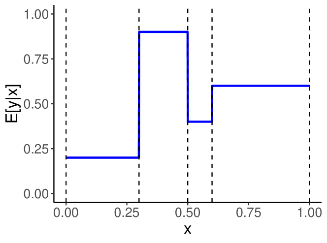
Figure 1: Regression tree (left) and implied regression function (right).

To extend this idea to additive regression trees, we consider not just one tree, but multiple trees $\mathcal{T}_{1},\ldots,\mathcal{T}_{m}$, each with their own corresponding partitions and leaf nodes. Then we let $\mathbb{E}[y_{i}\>|\>\mathbf{x}_{i}]\coloneqq\sum^{m}_{t=1}g(\mathbf{x}_{i},\mathcal{T}_{t},\mathcal{M}_{t})$. The definition of the statistical model now becomes

$$y_{i}=\sum^{m}_{t=1}g\left(\mathbf{x}_{i},\mathcal{T}_{t},\mathcal{M}_{t}\right)+\varepsilon_{i},$$

which is the basic BART model presented in Chipman et al. (2010). The model is typically not identified, since different sets of trees can lead to the same regression function. However, this is not a problem, since the individual trees are rarely of direct interest.

The sum of trees framework can also be used to model the conditional expectation of a binary response $\mathbf{y}$, which takes values in $\{0,1\}$. This is the probit BART model, again proposed originally in Chipman et al. (2010). The model is easier to present and analyse when it is cast in terms of a continuous latent variable. Suppose $\mathbf{z}$ is such that

$$y_{i}=\begin{cases}1&\text{ if }z_{i}>0\\ 0&\text{ otherwise}.\end{cases}$$ (2)

As before, we model $z_{i}$ as

$$z_{i}=\sum^{m}_{t=1}g\left(\mathbf{x}_{i},\mathcal{T}_{t},\mathcal{M}_{t}\right)+\varepsilon_{i}$$

with $\varepsilon_{i}\sim\text{N}(0,1)$. This then implies that

$$\mathbb{E}\left[y_{i}\>|\>\mathbf{x}_{i}\right]=\Pr\left(y_{i}=1\>|\>\mathbf{x}_{i}\right)=\Pr\left(z_{i}>0\>|\>\mathbf{x}\right)=\Phi\left(\sum_{t=1}^{m}g\left(\mathbf{x}_{i},\mathcal{T}_{t},\mathcal{M}_{t}\right)\right),$$

where $\Phi(\cdot)$ is the cumulative distribution function of the standard normal distribution.

For both types of outcome, given a sample of size $n$ and a univariate outcome vector $\mathbf{y}\in\mathbb{R}^{n}$ associated with a predictor matrix $\mathbf{X}\in\mathbb{R}^{n\times p}$, we are interested in sampling from the joint posterior distribution $\pi(\boldsymbol{\mathcal{T},\mathcal{M}}\>|\>\mathbf{y},\mathbf{X})$ where $\boldsymbol{\mathcal{T}}=(\mathcal{T}_{1},\ldots,\mathcal{T}_{m})$ denotes the collection of all trees and $\boldsymbol{\mathcal{{M}}}=(\mathcal{M}_{1},\ldots,\mathcal{M}_{m})$ denotes their corresponding mean parameters. To obtain the posterior, it is necessary to define priors for both the trees and the terminal node parameters. Assuming the independence of leaf parameters conditional on the tree structures, Chipman et al. (2010) defines the joint prior distribution as

$$\pi\left(\boldsymbol{\mathcal{T}},\boldsymbol{\mathcal{M}},\sigma^{2}\right) =\left[\prod_{t=1}^{m}\pi\left(\mathcal{T}_{t},\mathcal{M}_{t}\right)\right]\times\pi\left(\sigma^{2}\right)$$

$$=\left[\prod_{t=1}^{m}\pi\left(\mathcal{M}_{t}\>|\>{\mathcal{T}_{t}}\right)\times\pi\left(\mathcal{T}_{t}\right)\right]\times\pi\left(\sigma^{2}\right)$$

$$=\left[\prod_{t=1}^{m}\prod_{\ell=1}^{b_{m}}\pi\left(\mathcal{\mu}_{t\ell}\>|\>{\mathcal{T}_{t}}\right)\times\pi\left(\mathcal{T}_{t}\right)\right]\times\pi\left(\sigma^{2}\right).$$

To achieve conjugacy, it is typically assumed that the residual variance parameter $\sigma^{2}$ follows an inverse-gamma distribution and $\mu_{t\ell}\sim N(0,\sigma_{\mu}^{2})$. with $\sigma_{\mu}^{2}=\frac{0.25}{\kappa^{2}m}$ being proportional to the number of trees in order to regularise the contribution of each tree. The definition of $\pi(T_{t})$ includes specifying the probability of a non-terminal node as $\alpha(1+\gamma_{t\ell})^{-\beta}$ where $\gamma_{t\ell}$ denotes the depth of that node. The hyperparameters $\alpha$ and $\beta$ take the default values suggested in Chipman et al. (2010) of $0.95$ and $2$, respectively, to favour shallow trees.

Once the prior is defined, a sampler for the aforementioned posterior distribution can be obtained. Referring to $\boldsymbol{\mathcal{T}}_{(-t)}\coloneqq\boldsymbol{\mathcal{T}}\setminus\{\mathcal{T}_{t}\}$ and $\boldsymbol{\mathcal{M}}_{(-t)}\coloneqq\boldsymbol{\mathcal{M}}\setminus\{\mathcal{M}_{t}\}$, an MCMC sampler can be built by sequentially sampling $\pi(\mathcal{T}_{t}\>|\>\boldsymbol{\mathcal{T}}_{(-t)},\boldsymbol{\mathcal{M}},\mathbf{y},\mathbf{X},\sigma^{2})$ and $\pi(\mathcal{M}_{t}\>|\>\boldsymbol{\mathcal{T}},\boldsymbol{\mathcal{M}}_{(-t)},\mathbf{y},\mathbf{X},\sigma^{2})$. It can be shown that $\mathcal{T}_{t}$ and $\mathcal{M}_{t}$ depend on $(\boldsymbol{\mathcal{T}}_{(-t)},\mathbf{y})$ only through the partial residuals $\mathbf{r}_{t}\coloneqq\mathbf{y}-\sum_{j\neq t}^{m}g(\mathbf{X},\mathcal{T}_{j},\mathcal{M}_{j})$. This fact can be used to construct a Bayesian back-fitting algorithm (Hastie and Tibshirani, 2000). Therefore, the successive draws become

$\pi\left(\mathcal{T}_{t}\>|\>\mathbf{r}_{t},\sigma^{2}\right)$

$\pi\left(\mathcal{M}_{t}\>|\>\mathcal{T}_{t},\mathbf{r}_{t},\sigma^{2}\right)$,

where new trees and splitting rules are sampled through a Metropolis-Hastings step calculated using the integrated-likelihood for the tree $\mathcal{T}_{t}$ over the leaf parameters $\mathcal{M}_{t}$. See Chipman et al. (2010) and Kapelner and Bleich (2016) for further details of the model and additional information the algorithmic implementation on which that of the suBART models is based.

3.2 The suBART model for continuous outcomes

We consider a regression problem of the form

$$\begin{pmatrix}y_{i}^{(1)}\\ \vdots\\ y_{i}^{(d)}\end{pmatrix}=\begin{pmatrix}\mathbb{E}\left[y_{i}^{(1)}\>|\>\mathbf{x}_{i}\right]\\ \vdots\\ \mathbb{E}\left[y_{i}^{(d)}\>|\>\mathbf{x}_{i}\right]\end{pmatrix}+\begin{pmatrix}\varepsilon_{i}^{(1)}\\ \vdots\\ \varepsilon_{i}^{(d)}\end{pmatrix}$$ (3)

where $\mathbf{y}^{(j)}$ represents the $j$-th component of a $d$-variate outcome, and $(\varepsilon_{i}^{(1)},\ldots,\varepsilon_{i}^{(d)})^{\top}\sim\text{MVN}_{d}(\mathbf{0}_{d},\boldsymbol{\Sigma})$. In principle, different models can be used for each conditional expectation in Equation (3). If the conditional expectations are all assumed to be linear in $\mathbf{x}_{i}$, we obtain the classic SUR model (Zellner, 1962). We instead want to allow the possibility that the conditional expectations are non-linear. Given that the BART model has been shown to be a viable model in the one-dimensional setting, it seems reasonable to expect this viability to extend to the multivariate case. We therefore proceed by assigning an ensemble of regression trees to each $\mathbb{E}[y_{i}^{(j)}\>|\>\mathbf{x}_{i}]$ as follows:

$$\begin{pmatrix}y_{i}^{(1)}\\ \vdots\\ y_{i}^{(d)}\end{pmatrix}=\begin{pmatrix}\sum_{t=1}^{m}g\left(\mathbf{x}_{i},\mathcal{T}^{(1)}_{t},\mathcal{M}^{(1)}_{t}\right)\\ \vdots\\ \sum_{t=1}^{m}g\left(\mathbf{x}_{i},\mathcal{T}^{(d)}_{t},\mathcal{M}^{(d)}_{t}\right)\end{pmatrix}+\begin{pmatrix}\varepsilon_{i}^{(1)}\\ \vdots\\ \varepsilon_{i}^{(d)}\end{pmatrix},$$ (4)

where

• $\mathcal{T}^{(j)}_{t}$ is a binary tree which defines a finite partition $\{\mathcal{A}^{(j)}_{t\ell}:1\leq\ell\leq h^{(l)}_{t}\}$ of $\mathbb{R}^{p}$. Note that $h^{(j)}_{t}$ is the number of leaf nodes of the tree $\mathcal{T}^{(j)}_{t}$. The collection of all trees pertaining to the $j$-th outcome is denoted by $\boldsymbol{\mathcal{T}}^{(j)}=(\mathcal{T}_{1}^{(j)},\dots,\mathcal{T}_{m}^{(j)})$.

• $\mathcal{M}^{(j)}_{t}=(\mu^{(j)}_{t1},\ldots,\mu^{(j)}_{th^{(j)}_{t}})$ is the vector of leaf parameters associated with the tree $\mathcal{T}_{t}^{(j)}$. Similarly, the collection of all leaf parameters associated with the $j$-th outcome is denoted by $\boldsymbol{\mathcal{M}}^{(j)}$.

• $(\varepsilon_{i}^{(1)},\ldots,\varepsilon_{i}^{(d)})^{\top}\sim\text{MVN}_{d}(\mathbf{0}_{d},\boldsymbol{\Sigma})$, with $\boldsymbol{\Sigma}$ being a $d\times d$ covariance matrix. We write $\sigma^{2}_{j}\coloneqq\Sigma_{jj}$ for the diagonal elements, such that $\sigma^{2}_{j}$ is the variance of the error term $\boldsymbol{\varepsilon}^{(j)}$. We further write $\rho_{jk}\coloneqq\text{Cor}(\boldsymbol{\varepsilon}^{(j)},\boldsymbol{\varepsilon}^{(k)})\>\forall\>j\neq k$. Note that for any $j,k$, we have

  $$\rho_{jk}=\frac{\text{Cov}\left[\boldsymbol{\varepsilon}^{(j)},\boldsymbol{\varepsilon}^{(k)}\right]}{\sqrt{\text{Var}\left[\boldsymbol{\varepsilon}^{(j)}\right]\text{Var}\left[\boldsymbol{\varepsilon}^{(k)}\right]}}=\frac{\Sigma_{jk}}{\sqrt{\Sigma_{jj}\Sigma_{kk}}}=\frac{\Sigma_{jk}}{\sigma_{j}\sigma_{k}}.$$

The model setup is straightforward, and indeed similar to the original BART model in Chipman et al. (2010). Our model is comprised of $d$ univariate BART models, which are linked through the correlated error terms $\boldsymbol{\varepsilon}^{(j)}$. For simplicity, we assume that the number of trees $m$ is common across all $d$ outcomes. However, we stress that each submodel has its own separate collection of $m$ trees. Thus, there are $d\times m$ trees in total. This is a key difference compared to other multivariate BART versions (McJames et al., 2023; Um et al., 2023), which assume that the trees are the same for all outcomes, i.e., that there are only $m$ trees in which the leaf parameters associated with each tree are vectors $\boldsymbol{\mu}_{t\ell}$.

A consequence of this assumption in existing multivariate BART versions is the implication that the $p$-dimensional predictor $\mathbf{x}_{i}$ is the same for all $d$ outcomes. However, in systems of equations such as (3) and (4), the set of predictors $\mathbf{x}_{i}$ need not be of common dimension $p$ for each outcome. Indeed, our suBART software implementation allows different subsets of the predictors to be used for each constituent univariate BART model. Though we will henceforth assume that the predictors are the same for all outcomes, for simplicity, it is important to note that having the same set of predictors $\mathbf{x}_{i}$ available as candidates to form splitting rules in each set of trees does not imply that the trees for different outcomes will split on the same components of $\mathbf{x}_{i}$ at the same cutoff values. Unlike the standard SUR, imposing restrictions on the $\mathbf{x}_{i}$ for different outcomes is not required to ensure that different outcomes depend on different covariates under suBART, as different sets of trees will tend to form different partitions on different subsets of the feature space $\mathbf{X}$ anyway, by the inherent nature of the tree-generating process in BART. Although practitioners can impose such restrictions nonetheless, to strictly guarantee that the trees for a given outcome do not depend on certain predictors, this is an appealing property, in the sense that suBART minimises the need to pre-specify the parametric form of the models for each conditional expectation.

We assume that the $m$ regression trees for each outcome are all independent of each other and of the covariance matrix a priori, as per Chipman et al. (2010); i.e,

$$\pi\left(\left(\boldsymbol{\mathcal{T}}^{(1)},\boldsymbol{\mathcal{M}}^{(1)}\right),\ldots,\left(\boldsymbol{\mathcal{T}}^{(d)},\boldsymbol{\mathcal{M}}^{(d)}\right),\boldsymbol{\Sigma}\right)= \left(\prod^{m}_{t=1}\prod^{d}_{j=1}\pi\left(\mathcal{T}^{(j)}_{t},\mathcal{M}^{(j)}_{t}\right)\right)\times\pi\left(\boldsymbol{\Sigma}\right)$$

$$= \left(\prod^{m}_{t=1}\prod^{d}_{j=1}\pi\left(\mathcal{M}^{(j)}_{t}\>|\>\mathcal{T}^{(j)}_{t}\right)\pi\left(\mathcal{T}^{(j)}_{t}\right)\right)\times\pi\left(\boldsymbol{\Sigma}\right).$$

We further assume that the leaves of a tree are conditionally independent, given the tree structure, i.e.,

$$\pi\left(\mathcal{M}^{(j)}_{t}\>|\>\mathcal{T}^{(j)}_{t}\right)=\prod^{h^{(d)}_{t}}_{\ell=1}\pi\left(\mu^{(j)}_{t\ell}\>|\>\mathcal{T}^{(d)}_{j}\right).$$

With this setup, prior distributions for $\mathcal{T}^{(j)}_{t},\mu^{(j)}_{t\ell}$, and $\boldsymbol{\Sigma}$ are sufficient to specify the joint prior distribution for all model parameters. The tree structure $\mathcal{T}^{(j)}_{t}$ is assigned the same prior as in the original work by Chipman et al. (2010), with default hyperparameters $\alpha=0.95$ and $\beta=2$ to favour shallow trees and avoid over-fitting.

The prior used for the leaf node parameters is also aligned with the approach of standard BART. As noted earlier, this prior is formulated conditionally on the tree $\mathcal{T}^{(j)}_{t}$. We assume that each outcome component $\mathbf{y}^{(j)}$ is re-scaled such that $y^{(j)}_{i}\in[-0.5,0.5]$. This enables the model to specify, with defined probability, that the implicit prior for $\mathbb{E}[y^{(j)}_{i}\>|\>\mathbf{x}_{i}]$ lies within the rescaled interval. Consequently, the prior is then

$$\mu^{(j)}_{t\ell}\>|\>\mathcal{T}^{(j)}_{t}\sim\text{N}\left(0,{\sigma^{(j)}_{\mu}}^{2}\right),$$ (5)

where ${\sigma^{(j)}_{\mu}}^{2}=\frac{0.25}{\kappa^{2}m}$, as before. We suggest $\kappa=2$ as a default choice, which assigns a prior probability of $0.95$ to the event $\{\mathbb{E}[y_{i}^{(j)}\>|\>\mathbf{x}_{i}]\in[-0.5,0.5]\}$.

In the univariate BART model, the error variance is assigned an inverse-gamma prior, which is conditionally conjugate and can thus be easily incorporated into a Gibbs sampler. Furthermore, by choosing the hyperparameters accordingly, it is possible to put an informative prior on the error variance. The usual approach is as follows: suppose that for the outcome $\mathbf{y}$, we have a ‘data-based overestimate’ $\hat{\sigma}^{2}$ of the error variance $\sigma^{2}$ (for example, the sample variance of the observed $\mathbf{y}$ values). Presumably, the true value of $\sigma^{2}$ is smaller than $\hat{\sigma}^{2}$, since the variation of $\mathbf{y}$ is partly explained by the covariates $\mathbf{X}$. Therefore, we would like to assign a large prior probability to the event $\{\sigma^{2}<\hat{\sigma}^{2}\}$ (for example, $0.95$).

We now wish to generalise this idea to the multivariate setting: for all components $j$ of the outcome vector $\left(\mathbf{y}^{(1)},\ldots,\mathbf{y}^{(d)}\right)$, we have an overestimate $\hat{\sigma}^{2}_{j}$ of $\sigma^{2}_{j}$, and want to assign some probability $p$ to the event $\{\sigma^{2}_{j}<\hat{\sigma}^{2}_{j}\}$. Additionally, we also would like to control the prior on the correlations $\rho_{jk}$, where $j\neq k$. Since there is usually not strong prior information about these correlations, it is preferable for the prior to not be too informative in any direction. Additionally, the chosen solution should be computationally tractable and readily incorporated into MCMC samplers.

The inverse-Wishart distribution is often used as a prior for covariance matrices. As it is a straightforward multivariate generalisation of the inverse-gamma distribution, it facilitates easy computations. Unfortunately, the inverse-Wishart prior is not well-suited to meet our aforementioned goals; among other problems, it imposes a strong prior dependency between the variances and the correlations. Consequently, it is generally not feasible to choose the hyperparameters such that the prior has the desired properties for both the variances and the correlations. See Alvarez et al. (2014) for a detailed study of this issue.

We thus instead adapt an approach by Huang and Wand (2013) and parameterise the covariance matrix $\boldsymbol{\Sigma}$ as follows:

• $a_{j}\sim\text{Inv-Gamma}(1/2,1/A^{2}_{j})$, where $A_{j}>0$ is a fixed hyperparameter.

• $\boldsymbol{\Sigma}\>|\>a_{1},\ldots,a_{d}\sim\text{Inv-Wishart}_{d}(\nu+d-1,\mathbf{S}_{0})$, where $\mathbf{S}_{0}\coloneqq 2\nu\times\mbox{diag}\left(1/a_{1},\ldots,1/a_{d}\right)$.

The implied prior distribution for the correlations can be derived (Huang and Wand, 2013) and is given by

$$\pi\left(\rho_{jk}\right)=\left(1-\rho_{jk}^{2}\right)^{\frac{\nu}{2}-1},\quad\rho_{jk}\in\left(-1,1\right).$$ (6)

Crucially, the prior does not depend on $A_{1},\ldots,A_{d}$. It is uniform if and only if $\nu=2$. For higher values, the prior increasingly concentrates around zero. We consider $\nu=2$ a reasonable default choice, since we usually do not have any strong prior information on the correlations. In simulation tests, it was found that this uniform prior can sometimes lead to an ill-identified posterior, consequently causing problems with the MCMC sampling. This seems to occur primarily in situations where the sample size is small, the dimension of $\mathbf{X}$ is large, and the variability of the multivariate outcome is almost entirely explained by $\mathbf{X}$. In such cases, we have found it useful to increase $\nu$ to improve sampling. It is also worth recalling that the response vector is bivariate in the motivating CEA application in Section 2, such that there is only one such correlation parameter.

From the previous definitions, the prior for the standard deviations is given by $\sigma_{j}\sim\text{Half-$t$}(\nu,A_{j})$; see Wand et al. (2011) for more details. Since the priors for the correlations are independent of $A_{j}$, the choice of $A_{j}$ remains arbitrary. We can thus tweak it to enforce the prior probability $\Pr(\sigma_{j}<\hat{\sigma}_{j})=\alpha_{\sigma}$, in accordance with the standard BART approach. To do this, we set up the following equation

$$\alpha_{\sigma}=2\frac{\Gamma(\frac{\nu+1}{2})}{\Gamma(\frac{\nu}{2})\sqrt{\nu\pi A^{2}_{j}}}\int_{0}^{\hat{\sigma}_{j}}{\left(1+\frac{x^{2}}{\nu A^{2}_{j}}\right)}^{-\frac{\nu+1}{2}}\mathop{dx}$$ (7)

and solve it for $A_{j}$, which can be done through numerical root-finding. This expression is the cumulative distribution function of a Half-$t$-distributed random variable with degrees of freedom $\nu$, scale parameter $A_{j}$, and support on $[0,\infty)$. By rewriting Equation (7) in terms of regularised incomplete beta functions, it can be shown that this expression is continuous as well as strictly decreasing in $A_{j}$ and approaches $1$ and $0$ as $A_{j}$ approaches $0$ and $\infty$, respectively. Thus, the solution for $A_{j}$ exists and is unique.

3.3 Probit suBART

While the previous model was designed to jointly model multiple continuous outcome variables, we now turn our attention to binary outcomes. We will present a generalisation of the linear multivariate probit model (Chib and Greenberg, 1998), where the linear predictors are replaced by sums of regression trees. Alternatively, it can also be seen as a multivariate generalisation of the probit BART model.

Suppose that we have some predictor variables $\mathbf{X}$, and a binary outcome vector $\mathbf{y}_{i}^{(j)}\in\{0,1\}\>\forall\>j=1,\ldots,d$, whose dependence on $\mathbf{x}_{i}$ we want to model. In particular, we do not want to assume that the components of $\mathbf{y}_{i}$ are conditionally independent, given $\mathbf{x}_{i}$; there may be some leftover correlation which is not explained by $\mathbf{x}_{i}$. As in the basic probit BART model, we cast the multivariate version in terms of latent variables $\mathbf{z}_{i}=(z_{i}^{(1)},\ldots,z_{i}^{(d)})$; the construction is exactly as per Equation (2) for each outcome $j$. Then, the probit suBART model is given by

$$\begin{pmatrix}z_{i}^{(1)}\\ \vdots\\ z_{i}^{(d)}\end{pmatrix}=\begin{pmatrix}\sum_{t=1}^{m}g\left(\mathbf{x}_{i},\mathcal{T}^{(1)}_{t},\mathcal{M}^{(1)}_{t}\right)\\ \vdots\\ \sum_{t=1}^{m}g\left(\mathbf{x}_{i},\mathcal{T}^{(d)}_{t},\mathcal{M}^{(d)}_{t}\right)\end{pmatrix}+\begin{pmatrix}\varepsilon_{i}^{(1)}\\ \vdots\\ \varepsilon_{i}^{(d)}\end{pmatrix},$$ (8)

where

• $g(\cdot)$, $\mathcal{T}^{(j)}_{t}$, and $\mathcal{M}^{(j)}_{t}$ are defined as before.

• $(\varepsilon_{i}^{(1)},\ldots,\varepsilon_{i}^{(d)})^{\top}\sim\text{MVN}_{d}(\mathbf{0}_{d},\boldsymbol{\Sigma})$, with $\boldsymbol{\Sigma}$ being a $d\times d$ correlation matrix. Again writing $\rho_{jk}\coloneqq\text{Corr}(\boldsymbol{\varepsilon}^{(j)},\boldsymbol{\varepsilon}^{(k)})$ for $j\neq k$, we have

  $$\boldsymbol{\Sigma}_{jk}=\begin{cases}1&\text{if $j=k$}\\ \rho_{jk}&\text{if $j\neq k$}.\end{cases}$$

Conditional on the latent variables $\mathbf{z}_{i}$, the model is essentially the same as the suBART model presented earlier. The only difference is that for each error term $\boldsymbol{\varepsilon}^{(j)}$, we fix the variance at $1$. Without doing this, the model would be unidentified. This issue is not specific to probit suBART, but also arises in the linear multivariate probit model. See Chib and Greenberg (1998) for details. It follows that $\boldsymbol{\Sigma}$, the covariance matrix of the error terms, is equal to $1$ in each diagonal entry, and hence must be a correlation matrix.

The priors for the trees are exactly same as those for the suBART model. The dependence structure of the trees, leaves, and covariance matrix are also the same. The other priors are broadly similar, but there are some implications that are worth briefly highlighting. The prior for the terminal node parameters $\mu_{t\ell}^{(j)}$ again follows Equation (5), though the calibration of the variance hyperparameter requires more care. Taking ${\sigma^{(j)}_{\mu}}^{2}=\frac{q_{z}^{2}}{\kappa^{2}m}$, with $\kappa=2$ as a default choice, we assign a prior probability of $0.95$ to the event $\{\mathbb{E}[z_{i}^{(j)}\>|\>\mathbf{x}_{i}]\in[-q_{z},q_{z}]\}$. On the probability scale, this means that $\{\Pr(y_{i}^{(j)}=1)\in[\Phi(-q_{z}),\Phi(q_{z})]\}$. For example, when taking $q_{z}=3$ as per Chipman et al. (2010), we assign a prior probability of $0.95$ to the event $\{\Pr(y_{i}^{(j)}=1\>|\>\mathbf{x}_{i})\in[0.0013,0.9987]\}$. This is reasonable for many applications, since extremely small or large probabilities are uncommon.

In the probit setting, $\boldsymbol{\Sigma}$ is a correlation matrix and hence must be positive definite, as well as having all diagonal entries equal to $1$. These restrictions make it difficult to choose a prior for $\boldsymbol{\Sigma}$ which has desirable properties and facilitates easy sampling. Chib and Greenberg (1998) present a prior (and related sampling strategy) which we found to be extremely inefficient in our application. We thus instead adapt an approach by Zhang et al. (2006) (see also Barnard et al. (2000), where some of the following results originate, and Zhang (2020)). We introduce an auxiliary parameter $\mathbf{D}$, which is a $d\times d$ diagonal matrix. We then define $\mathbf{W}\coloneqq\mathbf{D}^{\frac{1}{2}}\boldsymbol{\Sigma}\mathbf{D}^{\frac{1}{2}}$, and assume the prior $\mathbf{W}\sim\text{Inv-Wishart}_{d}(\nu+d-1,\mathbf{I}_{d})$, where $\mathbf{I}_{d}$ is the $d$-dimensional identity matrix.

Given $\mathbf{W}$, we can recover $\mathbf{D}$ and $\boldsymbol{\Sigma}$ thanks to the identities $\mathbf{D}=\text{diag}(\mathbf{W})$ and $\boldsymbol{\Sigma}=\mathbf{D}^{-\frac{1}{2}}\mathbf{W}\mathbf{D}^{-\frac{1}{2}}$. The induced marginal prior density of $\boldsymbol{\Sigma}$ is

$$\pi\left(\boldsymbol{\Sigma}\right)\propto\left(\det\boldsymbol{\Sigma}\right)^{\frac{1}{2}(\nu+d-1)(d-1)-1}\left(\prod_{j=1}^{d}\det\left[\boldsymbol{\Sigma}\right]_{jj}\right)^{-\frac{\nu+d-1}{2}},$$

where $[\boldsymbol{\Sigma}]_{jj}$ is the $j$-th principle submatrix of $\boldsymbol{\Sigma}$. It can be shown that the marginal prior density for the correlations is again given by Equation (6), as per the suBART model for continuous outcomes above, despite the different priors assumed for $\boldsymbol{\Sigma}$. The hyperparameter $\nu$ plays a similar role as it did before; in most situations, we again consider $\nu=2$ a reasonable default choice but reiterate that higher values of $\nu$ may lead to more stable and efficient sampling in specific scenarios.

4 Posterior Inference

This section describes strategies and algorithmic details for conducting posterior inference under suBART and probit suBART for multivariate continuous and multivariate binary outcomes, respectively. For both frameworks, sampling is performed using a Metropolis-within-Gibbs sampler based on their respective priors and model specifications. Given an observed sample $\mathbf{y}_{1},\ldots,\mathbf{y}_{n}$, with $\mathbf{y}_{i}\in\mathbb{R}^{d}$, all computations are carried out conditionally on the covariates $\mathbf{X}\in\mathbb{R}^{n\times p}$. Thus, for the sake of readability, we will consider $\mathbf{X}$ fixed and not condition on it explicitly. Additionally, the expression $\pi(\theta\>|\>\Theta\setminus\{\ldots\})$ denotes the conditional distribution of $\theta$ with respect to all parameters except $\theta$ itself and the ones listed within the braces. For example, $\pi(\mathcal{T}^{(j)}_{t}\>|\>\Theta\setminus\{\mathcal{M}^{(j)}_{t}\})$ refers to the distribution of tree $\mathcal{T}^{(j)}_{t}$ given all parameters except $\mathcal{T}^{(j)}_{t}$ and $\mathcal{M}^{(j)}_{t}$. This slightly unusual notation reduces the complexity of the expressions which follow. Given that we routinely condition on all but two parameters, we find it clearer to highlight what is not being conditioned on.

4.1 suBART continuous

For brevity, we define the estimate for $y_{i}^{(j)}$ as $\hat{y}^{(j)}_{i}\coloneqq\linebreak{}\sum_{t=1}^{m}g(\mathbf{x}_{i},\mathcal{T}^{(j)}_{t},\mathcal{M}^{(j)}_{t})$ and $\mathbf{\hat{y}}_{i}=(\hat{y}_{i}^{(1)},\ldots,y^{(d)}_{i})^{\top}$, since there are now multiple components of $\mathbf{y}_{i}$. Analogously, we define the residuals from a tree $t$ associated with the $j$-th component as $\mathbf{r}^{(j)}_{t}\coloneqq\{r^{(j)}_{t1},\ldots,r^{(j)}_{tn}\}$, where $r^{(j)}_{ti}\coloneqq y^{(j)}_{i}-\sum_{k\neq t}^{m}g(\mathbf{x}_{i},\mathcal{T}^{(j)}_{k},\mathcal{M}^{(j)}_{k})$. As per the standard BART, we are interested in sampling from the posterior distribution

$$\pi(\Theta\>|\>\mathbf{Y})=\pi\left(\left(\boldsymbol{\mathcal{T}}^{(1)},\boldsymbol{\mathcal{M}}^{(1)}\right),\ldots,\left(\boldsymbol{\mathcal{T}}^{(d)},\boldsymbol{\mathcal{M}}^{(d)}\right),\boldsymbol{\Sigma},a_{1},\ldots,a_{d}\>|\>\mathbf{Y}\right),$$

which, due to the back-fitting algorithm (Hastie and Tibshirani, 2000) and properties of the multivariate normal distribution, can be obtained from sequential draws from a collection of conditional distributions. In the multivariate continuous outcomes setting, we have that $\mathbf{y}_{i}\sim\text{MVN}_{d}\left(\hat{\mathbf{y}}_{i},\boldsymbol{\Sigma}\right)$. For the following, we will also need the conditional distribution of any component $y^{(j)}_{i}$ given all other components $\mathbf{y}_{i}^{(-j)}$. Using a well-known result (see e.g., Baldi (2024), Section 4.4), this can be found in closed form:

$$y^{(j)}_{i}\>|\>\mathbf{y}^{(-j)}_{i},\Theta \sim\text{N}\left(\hat{y}_{i}^{(j)}+\boldsymbol{\Sigma}_{j(-j)}\boldsymbol{\Sigma}_{(-j)(-j)}^{-1}\left(\mathbf{y}^{(-j)}_{i}-\hat{\mathbf{y}}_{i}^{(-j)}\right),\right.$$

$$\phantom{\sim\text{N}}\left.\quad\!{\Sigma}_{jj}-\boldsymbol{\Sigma}_{j(-j)}\boldsymbol{\Sigma}_{(-j)(-j)}^{-1}\boldsymbol{\Sigma}_{(-j)j}\right),$$ (9)

where $\boldsymbol{\Sigma}_{(-j)(-j)}$ is the submatrix obtained by excluding the $j$-th row and column. Analogously, $\boldsymbol{\Sigma}_{j(-j)}$ denotes the vector obtained by selecting the $j$-th row and excluding the $j$-th column from $\boldsymbol{\Sigma}$. Using the result from Equation (9), the posterior distribution $\pi(\mathcal{T}^{(j)}_{t}\>|\>\mathbf{r}^{(j)},\Theta\setminus\{\mathcal{M}_{t}^{(j)}\})$ can also be obtained in closed-form, up to a normalising constant, as the conditional distribution of the residual component $r_{i}^{(j)}$ given $\hat{\mathbf{y}}_{i}^{(-j)}$ is known. Then, as described in Section 3.1, the sampler for the joint posterior distribution of the trees $\mathcal{T}^{(j)}_{t}$ and their parameters $\mathcal{M}_{t}^{(j)}$, for the $j$-th component of $\mathbf{y}^{(1)},\ldots,\mathbf{y}^{(d)}$, is given by successive draws from

$\mathcal{T}^{(j)}_{t}\>|\>\mathbf{r}^{(j)}_{t},\Theta\setminus\left\{\mathcal{M}_{t}^{(j)}\right\}$

$\mathcal{M}^{(j)}_{t}\>|\>\mathbf{r}^{(j)}_{t},\Theta.$

Notably, the algorithm reduces to the standard BART approach when the dimension $d$ is equal to one. Indeed, each draw above can also be viewed as univariate BART — albeit with distinct mean and variance parameters — since it is conditioned on the values of all other components in $\mathbf{Y}$, as illustrated by Equation (9). The full structure of the suBART sampler is given in Algorithm 1, but we first describe the remaining required posterior conditional distributions.

The posterior distribution for $\mu^{(j)}_{t\ell}$ is given by

$$\mu^{(j)}_{t\ell}\>|\>\Theta\sim\text{N}\left(\left(\frac{{\sigma_{\mu}^{(j)}}^{2}}{v^{(j)}+n_{t\ell}^{(j)}{\sigma_{\mu}^{(j)}}^{2}}\right)\times\left(\sum_{i=1}^{n_{t\ell}^{(j)}}r_{i}^{(j)}-\sum_{i=1}^{n_{t\ell}^{(j)}}u_{i}^{(j)}\right),\frac{v^{(j)}{\sigma_{\mu}^{(j)}}^{2}}{v^{(j)}+n_{t\ell}^{(j)}{\sigma_{\mu}^{(j)}}^{2}}\right),$$ (10)

where $u_{i}^{(j)}\coloneqq\boldsymbol{\Sigma}_{j(-j)}\boldsymbol{\Sigma}_{(-j)(-j)}^{-1}(\mathbf{y}^{(-j)}_{i}-\hat{\mathbf{y}}_{i}^{(-j)})$, $v^{(j)}\coloneqq\Sigma_{jj}-\boldsymbol{\Sigma}_{j(-j)}\boldsymbol{\Sigma}_{(-j)(-j)}^{-1}\boldsymbol{\Sigma}_{(-j)j}$, and $n_{t\ell}^{(j)}$ denotes the number of observations in the indicated terminal node. It is evident from Equation (10) that the term $u_{i}^{(j)}$ vanishes and $v^{(j)}=\sigma_{\mu}^{2}$ when $d=1$, resulting in an expression identical to the original BART formulation.

Thanks to the conditional conjugacy in the construction due to Huang and Wand (2013), the conditional posteriors of $\boldsymbol{\Sigma}$ and the auxiliary parameters $a_{1},\ldots,a_{d}$ take simple forms. We have

$$a_{j}\>|\>\Theta\sim\text{Inv-Gamma}\left(\frac{\nu+n}{2},\frac{1}{A^{2}_{j}}+\nu\left(\boldsymbol{\Sigma}^{-1}\right)_{jj}\right),$$ (11)

where $(\boldsymbol{\Sigma}^{-1})_{jj}$ denotes the $j$-th entry along the diagonal of $\boldsymbol{\Sigma}^{-1}$, and

$$\boldsymbol{\Sigma}\>|\>\Theta\sim\text{Inv-Wishart}_{d}\left(\nu+n,\mathbf{S}_{0}+\mathbf{S}\right),$$ (12)

where $\mathbf{S}=\sum_{i=1}^{n}(\mathbf{y}_{i}-\hat{\mathbf{y}}_{i})(\mathbf{y}_{i}-\hat{\mathbf{y}}_{i})^{\top}.$ A detailed derivation of the latter result can be found in Hoff (2009).

Input: $\mathbf{X}$, $\mathbf{Y}$, $m$, $N_{\text{MCMC}}$, $N_{\text{burn-in}}$, and all hyper-parameters of the priors.

Initialise: $\boldsymbol{\mathcal{T}}^{(1)},\ldots,\boldsymbol{\mathcal{T}}^{(d)}$ tree stumps, $\boldsymbol{\Sigma}$, $\mu^{(j)}_{t\ell}=0\>\forall\>(t,j)$.

1 for iterations $h$ from $1$ to $N_{\text{MCMC}}$ do

2       for dimension $j$ from $1$ to $d$ do

3             for trees $t$ from $1$ to $m$ do

4                   Calculate the partial residuals $\mathbf{r}^{(j)}_{t}$;

5                   Propose a new tree ${\mathcal{T}^{(j)}_{t}}^{\star}$ by a grow, prune, or change move;

6                   Accept and update $\mathcal{T}^{(j)}_{t}={\mathcal{T}^{(j)}_{t}}^{\star}$ with probability

$$\gamma^{\star}\left(\mathcal{T}^{(j)}_{t},{\mathcal{T}_{t}^{(j)}}^{\star}\right)=\min\left\{1,\frac{\pi\left(\mathbf{R}^{(j)}_{t}\>|\>{\mathcal{T}_{t}^{(j)}}^{\star},\Theta\setminus\left\{M_{t}^{(j)}\right\}\right)\pi\left({\mathcal{T}_{t}^{(j)}}^{\star}\right)}{\pi\left(\mathbf{R}_{t}\>|\>{\mathcal{T}_{t}^{(j)}},\Theta\setminus\left\{M_{t}^{(j)}\right\}\right)\pi\left({\mathcal{T}_{t}^{(j)}}\right)}\right\}.$$

for terminal nodes $\ell$ from $1$ to $b^{(j)}_{t}$ do

7                         Update $\mu^{(j)}_{t\ell}\>|\>\mathbf{r}_{t}^{(j)},\Theta$ using Equation (10).

8                   end for

9                  

10             end for

11            

12       end for

13       for  $j$ from $1$ to $d$ do

14             Update $a_{j}\>|\>\Theta$ using Equation (11).

15       end for

16       Update $\boldsymbol{\Sigma}\>|\>\Theta$ using Equation (12).

17 end for

Algorithm 1 suBART sampling algorithm.

4.2 Probit suBART

In the multivariate binary setting, the goal is to draw samples from the similar posterior

$$\pi(\Theta\>|\>\mathbf{Y})=\pi\left(\left(\boldsymbol{\mathcal{T}}^{(1)},\boldsymbol{\mathcal{M}}^{(1)}\right),\ldots,\left(\boldsymbol{\mathcal{T}}^{(d)},\boldsymbol{\mathcal{M}}^{(d)}\right),\boldsymbol{\Sigma},\mathbf{D}\>|\>\mathbf{Y}\right).$$

Note that $\mathbf{W}$ is a deterministic function of $\boldsymbol{\Sigma}$ and $\mathbf{D}$, and is hence omitted from the above distribution. However, it will be more convenient to work with the joint posterior of the parameters and the latent variables

$$\pi\left(\Theta,\mathbf{Z}\>|\>\mathbf{Y}\right)=\pi\left(\left(\boldsymbol{\mathcal{T}}^{(1)},\boldsymbol{\mathcal{M}}^{(1)}\right),\ldots,\left(\boldsymbol{\mathcal{T}}^{(d)},\boldsymbol{\mathcal{M}}^{(d)}\right),\boldsymbol{\Sigma},\mathbf{D},\mathbf{Z}\>|\>\mathbf{Y}\right),$$

for which the sampling algorithm is very similar to the previously presented Algorithm 1 in the continuous setting. For brevity, we discuss only the required modifications to Algorithm 1 without presenting a new algorithm in full.

The updates for the trees and leaf nodes stay essentially the same, with the one difference being that the latent variables $\mathbf{Z}$ replace the data $\mathbf{Y}$. The updates for the $a_{j}$ parameters are of course dropped, since they do not apply to the probit model. An important additional step is that the latent variables for each component $j$ should be updated after line 9 in Algorithm 1. In a similar manner to Equation (9), the marginal distribution of $z_{i}^{(j)}$ can be obtained via

$$z^{(j)}_{i}\>|\>\mathbf{z}^{(-j)}_{i},\Theta \sim\text{N}\left(\hat{z}_{i}^{(j)}+\boldsymbol{\Sigma}_{j(-j)}\boldsymbol{\Sigma}_{(-j)(-j)}^{-1}\left(\mathbf{z}^{(-j)}_{i}-\hat{\mathbf{z}}_{i}^{(-j)}\right),\right.$$

$$\phantom{\sim\text{N}}\left.\quad\!{\Sigma}_{jj}-\boldsymbol{\Sigma}_{j(-j)}\boldsymbol{\Sigma}_{(-j)(-j)}^{-1}\boldsymbol{\Sigma}_{(-j)j}\right).$$ (13)

However, sampling the latent variables also requires conditioning on $\mathbf{Y}$. In doing so, we find that $\pi(z^{(j)}_{i}\>|\>\mathbf{z}^{(-j)}_{i},\mathbf{Y},\Theta)$ follows a truncated normal distribution with the same location and scale parameters as Equation (13). However, we encounter a case distinction for the support of this conditional posterior distribution based on the values of the associated response. If $y_{i}^{(j)}=0$, which implies that $z_{i}^{(j)}\leq 0$, the support is truncated to $(-\infty,0]$. Conversely, if $y_{i}^{(j)}=1$, which implies that $z_{i}^{(j)}>0$, the support is truncated to $(0,\infty)$. In each case, we draw the sample through the method proposed by Robert (1995).

Finally, the other major difference for the probit suBART sampler is the update of $\boldsymbol{\Sigma}$ and the auxiliary parameter $\mathbf{D}$ . We write out the conditional posterior as

$$\pi\left(\boldsymbol{\Sigma},\mathbf{D}\>|\>\Theta,\mathbf{Z}\right) \propto\pi\left(\boldsymbol{\Sigma},\mathbf{D}\right)\left(\det\mathbf{D}\right)^{\frac{d-1}{2}}\pi\left(\mathbf{Z}\>|\>\Theta\right)$$

$$\propto\pi\left(\boldsymbol{\Sigma},\mathbf{D}\right)\left(\det\mathbf{D}\right)^{\frac{d-1}{2}}\left(\det\boldsymbol{\Sigma}\right)^{-n/2}\exp\left(-\frac{1}{2}\sum_{i=1}^{n}\left(\mathbf{z}_{i}-\hat{\mathbf{z}}_{i}\right)^{\top}\boldsymbol{\Sigma}^{-1}\left(\mathbf{z}_{i}-\hat{\mathbf{z}}_{i}\right)\right),$$

where $\pi(\boldsymbol{\Sigma},\mathbf{D})=\pi(\mathbf{W})$ is the aforementioned inverse-Wishart prior on $\mathbf{W}$. The term $(\det\mathbf{D})^{\frac{d-1}{2}}$ is the Jacobian determinant which arises due to the change of variables $\mathbf{W}\mapsto\boldsymbol{\Sigma},\mathbf{D}$. This distribution is not of known form, and can hence cannot be sampled from directly. We instead proceed using the parameter-expanded Metropolis-Hastings (PX-MH) algorithm of Zhang (2020). This defines a proposal for $\mathbf{W}^{(k+1)}\>|\>\mathbf{W}^{(k)},\nu_{\text{prop}}\sim\text{Inv-Wishart}_{d}\left(\nu_{\text{prop}},\mathbf{W}^{(k)}\right)$ where $k$ is the current MCMC iteration and $\nu_{\text{prop}}$ is a tuning parameter.

5 Simulation studies

In this section, we evaluate the efficacy of the proposed models through experiments with simulated data. Section 5.1 and Section 5.2 are devoted to simulation designs in which the responses $\mathbf{y}^{(1)},\ldots,\mathbf{y}^{(d)}$ are all continuous and each outcome $\mathbf{y}^{(j)}\in\{0,1\}$ is binary, respectively. We undertake a comparative analysis of suBART against benchmark models, including the standard BART model, the multivariate BART (mvBART) model, and a Bayesian linear seemingly unrelated regression (SUR) model. We also consider probit versions of each model, where available. This comparative study aims to explore various aspects of the models, including predictive performance and their ability to accommodate assumptions regarding correlation among responses and/or assumptions of linearity. Furthermore, our simulations aim to elucidate the primary distinctions between the suBART and mvBART approaches. For example, the splits generated by trees within the mvBART framework entail a splitting rule in all components of $\mathbf{Y}$, potentially deviating from an accurate representation of the true function $f(\mathbf{X})$ for some scenarios. Consequently, each response variable in our experiments is generated using a different subset of covariates. Additionally, a significant improvement in predictive performance capacity should be anticipated when compared with the linear SUR model as, for the most part, the responses in our experiments are almost all assumed to be non-linearly related to the covariates.

These assumptions were tested over $100$ replications of each simulation scenario, using different sample sizes of $n_{\text{train}}=n_{\text{test}}=\{250,500,1000\}$ for training and test samples respectively. The metrics employed to assess differences in model performance included the root mean squared error (RSME), the continuous ranked probability score (CRPS; Gneiting and Raftery, 2007), and the prediction interval (PI) coverage for the multivariate regression cases, while the logarithmic loss, the accuracy (ACC), and the credible interval coverage of the probabilities from $\Phi(z_{i}^{(j)})$ were used for the multivariate probit scenarios. The 50% posterior intervals are computed using the 25-th and 75-th percentiles over the posterior samples from $\hat{Y}_{i}^{(j)}$, while the posterior means for each $\hat{Y}_{i}^{(j)}$, $\sigma_{j}$, and $\rho_{jk}$ are obtained by averaging the posterior replications.

Throughout all experiments, the default choice for the inverse-Wishart hyperparameter is $\nu=2$, reflecting our lack of prior information about the correlation structure (Huang and Wand, 2013). The selection of the proposal degrees of freedom $\nu_{\text{prop}}$ for the PX-MH algorithm can be fine-tuned to adjust its acceptance rate, as outlined in prior studies (Zhang et al., 2006). Consistent with existing literature such as Zhang et al. (2015), we adopt the default value of $\nu_{\text{prop}}=n_{\text{train}}$, which appears to ensure a sufficiently well-behaved sampler. The number of trees for each component $j$ was fixed at $m=50$. For the MCMC settings, we set a total of $N_{\text{MCMC}}=3000$ iterations, of which $N_{\text{burn-in}}=1000$ samples are discarded as burn-in. Adjustments to the number of MCMC samples and other hyperparameters such as $\nu$, $\nu_{\text{prop}}$, and $m$ could be made to enhance convergence and predictive performance, although the model does not appear to be overly sensitive to such variations.

Lastly, we note the software implementations for each model included in the comparison. The suBART models are fitted using our own suBART implementation and the BART models are fitted using the dbarts package (Dorie et al., 2024), while the linear Bayesian SUR models (henceforth BayesSUR) were implemented using the probabilistic programming language Stan (Stan Development Team, 2024b), through the rstan package (Stan Development Team, 2024a) which provides an R interface for this library. The mvBART model was evaluated using the skewBART implementation provided by Um et al. (2023), specifically by setting the argument do_skew=FALSE of the main MultiskewBART() function. However, it is worth noting that its current implementation is limited to continuous scenarios with two dimensions, thereby results were constrained to such cases. The default arguments were retained for all competing models with the exception of the number of trees for the tree-based models, which were set to the same value ($m=50$) as suBART.

5.1 Continuous response experiments

The two simulation scenarios described by the systems of equations below were created to accommodate different types of complexity. In these experiments, the values of the response are non-linear functions modified from examples described in Friedman (1991) and Breiman (1996) for a multivariate response scenario. In the first scenario, the third response is exceptional in the sense that the generating function is purely linear. Note that correlated noise $(\varepsilon_{i}^{(1)},\ldots,\varepsilon_{i}^{(d)})^{\top}\sim\text{MVN}_{d}(\mathbf{0}_{d},\boldsymbol{\Sigma})$ is subsequently added to the $d$-dimensional response in each scenario.

Friedman #1:

$$x^{(1)}_{i},\ldots,x_{i}^{(10)}\overset{\mathrm{iid}}{\sim}\text{Uniform}(0,1)$$

$$y_{i}^{(1)}=10\sin\left(x_{i}^{(1)}x_{i}^{(2)}\pi\right)+20\left(x_{i}^{(3)}-0.5\right)^{2}$$

$$y_{i}^{(2)}=8x_{i}^{(4)}+20\sin\left(x_{i}^{(1)}\pi\right)$$

$$y_{i}^{(3)}=10x_{i}^{(5)}-5x_{i}^{(2)}-5x_{i}^{(4)}$$

Friedman #2:

$$x_{i}^{(1)},\ldots,x_{i}^{(5)},x_{i}^{(8)},x_{i}^{(10)}\overset{\mathrm{iid}}{\sim}\text{Uniform}(0,1)$$

$$x_{i}^{(6)}\sim\text{Uniform}(0,100)$$

$$x_{i}^{(7)}\sim\text{Uniform}(40\pi,560\pi)$$

$$x_{i}^{(9)}\sim\text{Uniform}(1,11)$$

$$y_{i}^{(1)}=10\sin\left(x_{i}^{(1)}x_{i}^{(2)}\pi\right)+20\left(x_{i}^{(3)}-0.5\right)^{2}+10x_{i}^{(4)}+5x_{i}^{(5)}$$

$$y_{i}^{(2)}=\sqrt{{x_{i}^{(6)}}^{2}+\left(x_{i}^{(7)}x_{i}^{(8)}-\frac{1}{{x_{i}^{(7)}x_{i}^{(9)}}}\right)^{2}}$$

$$y_{i}^{(3)}=\text{atan}\left(\frac{{x_{i}^{(7)}x_{i}^{(8)}-\frac{1}{{x_{i}^{(7)}x_{i}^{(9)}}}}}{{x_{i}^{(6)}}}\right)$$

The $p=10$ predictors are generated from a uniform distribution in each scenario. It is notable that not all predictors are used to build the responses. However, all $p=10$ predictors are used for model fitting in each case. It is anticipated that the tree-based models will be able to identify these uninformative noise variables. It is also essential to emphasise that each component of the outcome vector $\mathbf{Y}$ is derived from a distinct set of predictors in both scenarios. However, no restrictions are imposed on which predictors are associated with which response during model fitting. As previously mentioned, it is anticipated that mvBART may encounter challenges in accurately approximating the true generating functions in such cases. For each tree, the partitioning of the covariate space is reflected across all responses, which may not hold true, particularly when examining the responses of the Friedman #2 scenario where $y^{(1)}$ and $y^{(2)}$ do not share any predictors.

In each simulated scenario, we varied the dimension of the covariance error matrix within $d=\{2,3\}$ and defined $\boldsymbol{\Sigma}$ accordingly, with specific values assigned to each parameter $\sigma_{j}$ and each correlation parameter $\rho_{jk}$, for all $j\neq k$. In both Friedman scenarios, the error covariance parameters were set as detailed in Table 1 and it is the first two responses $y_{i}^{(1)}$ and $y_{i}^{(2)}$ which comprise the $d=2$ settings. The restriction to $d=2$ enables consideration of the mvBART model in the comparisons, owing to the aforementioned limitation of the skewBART software to bivariate outcome settings.

Table 1: True parameters of $\boldsymbol{\Sigma}$ used for each simulation scenario.

	$d$	$\sigma_{1}$	$\sigma_{2}$	$\sigma_{3}$	$\rho_{12}$	$\rho_{13}$	$\rho_{23}$
Friedman #1	$2$	$1.00$	$10.00$	—	$0.75$	—	—
	$3$	$1.00$	$2.50$	$5.00$	$0.80$	$0.50$	$0.25$
Friedman #2	$2$	$1.00$	$125.00$	—	$0.75$	—	—
	$3$	$1.00$	$125.00$	$0.10$	$0.80$	$0.50$	$0.25$

A comparison of results is depicted in the boxplots in Figure 2 and Figure 3 which confirm previous assumptions about suBART performance. These figures illustrate the results for Friedman #1 with $n_{\text{train}}=n_{\text{test}}=1000$. In general, suBART exhibits either slightly superior or competitive predictive performance when compared to BART and mvBART, as evidenced by small average values of RMSE and CRPS over the test samples. Furthermore, when compared with BayesSUR, all tree-based methods exhibit a clear superiority in estimating the non-linear responses. The primary discrepancy occurs when $j=3$, where BayesSUR has the best performance owing to the linearity of this response.

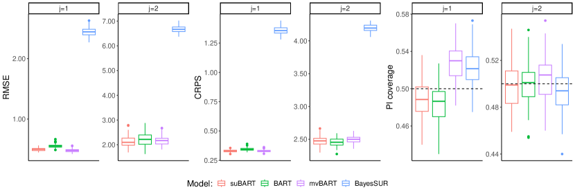
Figure 2: Simulation results for continuous outcomes for Friedman #1 with $n_{\text{train}}=n_{\text{test}}=1000$ and $d=2$.

In terms of uncertainty estimation, Figure 2 illustrates that all methods exhibit reasonable coverage ratios when $d=2$, except for the first component where both mvBART and linear SUR displayed higher coverage ratios for the prediction intervals, indicating that $\sigma_{1}^{2}$ was overestimated. Figure 3 corroborates these findings, with the divergence observed only when the response is solely dictated by a linear function, as illustrated by panels with $j=3$ in Figure 3.

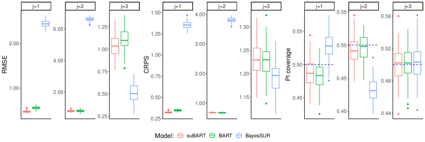
Figure 3: Simulation results for continuous outcomes for Friedman #1 with $n_{\text{train}}=n_{\text{test}}=1000$ and $d=3$.

For the Friedman #2 scenario, the results are summarised in Figure 4 where $d=2$ and $n_{\text{train}}=n_{\text{test}}=1000$. In this case, suBART consistently outperforms its competitors in all aspects. The deteriorated performance of mvBART can be explained by the particular nature of the simulation setting, where each outcome relates to an entirely distinct set of predictors, while the tree splits assume the opposite. Additionally, the calibration of the suBART estimations remains consistent, as evidenced by the boxplot for the PI coverage, which mostly covers the correct value. Equivalent figures summarising the results for the remaining scenarios, with $d=3$ and/or different sample sizes, yield the same conclusions as above and have been omitted for brevity; they can be found in the Appendix.

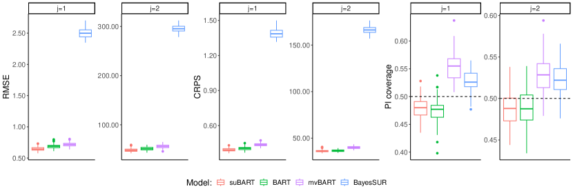
Figure 4: Simulation results for continuous outcomes for Friedman #2 with $n_{\text{train}}=n_{\text{test}}=1000$ and $d=2$.

Ultimately, for proper uncertainty calibration, it is essential to correctly estimate the correlation values from the covariance matrix $\boldsymbol{\Sigma}$. Table 1 displays the RMSE and coverage ratio of a 50% credible interval (CI) for the correlation parameters $\rho_{jk}$ for all $j\neq k$ provided by suBART, mvBART, and BayesSUR. Notably, correlation values for the BART model are not provided as it assumes independence among multiple responses (i.e., $\hat{\rho}_{jk}=0\>\forall\>j\neq k$), and the mvBART estimations are restricted when $d=2$ due to limitations of the skewBART package. From the results, it is clear that suBART outperforms mvBART and BayesSUR in terms of coverage, demonstrating its superior ability to estimate correlation structures. The coverage values of zero for BayesSUR are particularly notable and suggest an inability to accurately estimate correlations when assuming linear regressions for non-linear responses. In terms of RMSE, suBART is superior to BayesSUR and comparable to mvBART, albeit only in the $d=2$ setting.

Table 2: RMSE and coverage of a 50% CI for $\bar{{\rho}}_{jk}$ from the posterior samples for Friedman #1 with $n_{\text{train}}=n_{\text{test}}=1000$ for continuous outcomes.

	RMSE			CI coverage
	suBART	mvBART	BayesSUR	suBART	mvBART	BayesSUR
$d=2$
$\rho_{12}$	$0.02$	$0.02$	$0.33$	$0.50$	$0.05$	$0.00$
$d=3$
$\rho_{12}$	$0.02$	—	$0.37$	$0.37$	—	$0.00$
$\rho_{13}$	$0.03$	—	$0.31$	$0.41$	—	$0.00$
$\rho_{23}$	$0.03$	—	$0.18$	$0.52$	—	$0.00$

5.2 Binary response experiments

The experiments for binary responses are aligned with those from Section 5.1, wherein different sample sizes of $n_{\text{train}}=n_{\text{test}}=\{250,500,1000\}$ are used for training and test samples respectively. The simulation of the latent variables $z^{(j)}$ is described by the system of equations below. Other than when $j=3$, the values of the latent variables are non-linear functions. Recall that correlated noise $(\varepsilon_{i}^{(1)},\ldots,\varepsilon_{i}^{(d)})^{\top}\sim\text{MVN}_{d}(\mathbf{0}_{d},\boldsymbol{\Sigma})$ is subsequently added to the $d$-dimensional latent variable, where the true $\boldsymbol{\Sigma}$ parameters are set to the same values as Table 1, and that the generating process for each binary response follows Equation (2) thereafter.

Friedman #3:

$$x_{i}^{(1)},\ldots,x_{i}^{(10)}\overset{\mathrm{iid}}{\sim}\text{Uniform}(0,1)$$

$$z_{i}^{(1)}=\sin\left(x_{i}^{(1)}x_{i}^{(2)}\pi\right)+{x_{i}^{(3)}}^{3}$$

$$z_{i}^{(2)}=-1+2x_{i}^{(1)}x_{i}^{(4)}+e^{x_{i}^{(5)}}$$

$$z_{i}^{(3)}=0.5\left(x_{i}^{(2)}+x_{i}^{(4)}\right)+x_{i}^{(5)}$$

The models evaluated for these experiments are the probit suBART and probit extensions of the standard BART and BayesSUR. Despite the complete unavailability of a probit version of mvBART in the skewBART software, for any dimensionality, we persist in evaluating settings with varying dimension $d=\{2,3\}$ with the $d=2$ setting again comprising the first two responses. The results are summarised in Figure 5 and Figure 6, which are consistent with the findings from Section 5.1. When logarithm loss and ACC are considered as metrics for evaluating predictive performance, suBART either exhibits superior results or comparable averages. Both tree-based models outperform Bayesian SUR, with the exception of the linear third response in the $d=3$ setting, as per the earlier continuous simulation studies in Section 5.1.

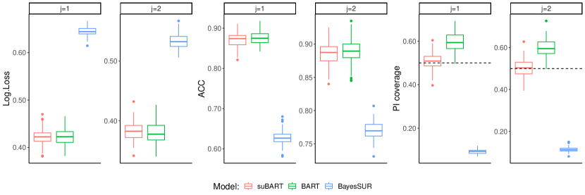
Figure 5: Simulation results for binary outcomes for Friedman #3 with $n_{\text{train}}=n_{\text{test}}=1000$ and $d=2$.

Regarding calibration, it is evident that suBART outperforms BART across all scenarios, showing coverage ratios that closely approximate the true values. On the other hand, due to the inherent linearity of BayesSUR, its calibration performance is notably poorer, though the third linear response is again an exception in this regard, as per Section 5.1. However, even for this linear response, suBART appears to exhibit superior performance in uncertainty quantification when compared to standard BART. For brevity, the results for remaining sample sizes are presented in the Appendix, as they lead to similar conclusions.

Figure 6: Simulation results for binary outcomes for Friedman #3 with $n_{\text{train}}=n_{\text{test}}=1000$ and $d=3$.

The results regarding the estimation of the correlation parameters are presented in Table 3, which includes the RMSE and CI coverage for the correlation parameters $\rho_{jk}$ associated with binary responses when $n_{\text{train}}=1000$. These results are consistent with Table 2 in clearly demonstrating superior performance of suBART with respect to prediction accuracy and estimating correlation structures.

Table 3: RMSE and coverage of a 50% CI for $\bar{{\rho}}_{jk}$ from the posterior samples for Friedman #3 with $n_{\text{train}}=n_{\text{test}}=1000$ for binary outcomes.

	RMSE		CI coverage
	suBART	BayesSUR	suBART	BayesSUR
$d=2$
$\rho_{12}$	$0.25$	$0.51$	$0.42$	$0.00$
$d=3$
$\rho_{12}$	$0.04$	$0.27$	$0.46$	$0.00$
$\rho_{13}$	$0.05$	$0.11$	$0.47$	$0.06$
$\rho_{23}$	$0.06$	$0.08$	0$.47$	$0.32$

6 Analysis of the TTCM data

We now apply the continuous suBART model in the cost-effectiveness setting which we introduced in Section 2. We analyse data from Wiertsema et al. (2019). The authors collected data on $n=140$ patients suffering from traumatic injuries. The two treatment options are usual care and the novel transmural trauma care model (TTCM), denoted by $t=0$ and $t=1$, respectively. The treatment assignment was not randomised. The outcomes we use, for $c$ and $q$ respectively, are the costs from the healthcare perspective and generic healthcare-related quality of life.

As is usual in CEAs, the cost outcome is an aggregate measure: $c$ comprises the total costs acquired from hospital records as well as several questionnaires conducted over the course of nine months following treatment, in which patients were surveyed on their use of various healthcare resources. The responses — examples of which relate to issues such as hospital stays, medication use, and surgeries — were then converted to costs. Conversely, the effectiveness outcome $q$ was calculated from one single survey administered nine months after treatment using the EQ-5D-3L instrument (Lamers et al., 2006). Additional details on the data collection process can be found in Wiertsema et al. (2019). The data also includes $p=11$ baseline covariates, with respective sample sizes of $83$ and $57$ in the two treatment groups. The ratio of covariates to observations is thus reasonably large. We reproduce the table of baseline variables in Table 4. We account for the categorical predictors in the tree-based models using the method of ordering categories proposed by Breiman et al. (1984).

Table 4: Baseline data from Wiertsema et al. (2019).

Characteristics	Mean (SD) or frequency (%)
	Intervention group ($t=1$)	Control group ($t=0$)
$n$	$83$	$57$
Age	$43.4~{}(15.6)$	$50.5~{}(17.9)$
Gender (M/F)	$39/44~{}(47/53\%)$	$26/31~{}(46/54\%)$
Education level
Low	$7~{}(8.4\%)$	$6~{}(11.1\%)$
Middle	$19~{}(22.9\%)$	$16~{}(29.6\%)$
High	$57~{}(68.7\%)$	$32~{}(59.3\%)$
Medical history
None	$53~{}(63.9\%)$	$30~{}(52.6\%)$
Chronic	$14~{}(16.9\%)$	$13~{}(22.8\%)$
Musculoskeletal	$16~{}(19.3\%)$	$14~{}(24.6\%)$
Trauma type
Traffic	$44~{}(53.0\%)$	$25~{}(43.9\%)$
Work related	$0~{}(0.0\%)$	$2~{}(3.5\%)$
Fall	$27~{}(32.5\%)$	$17~{}(29.8\%)$
Sports	$11~{}(13.3\%)$	$9~{}(15.8\%)$
Other	$1~{}(1.2\%)$	$4~{}(7.0\%)$
Fracture region
Upper extremity	$31~{}(37.3\%)$	$25~{}(43.9\%)$
Lower extremity	$41~{}(49.4\%)$	$19~{}(33.0\%)$
Vertebral	$7~{}(8.4\%)$	$1~{}(1.8\%)$
Multitrauma	$4~{}(4.8\%)$	$12~{}(21.1\%)$
Injury severity score	$7.9~{}(4.4)$	$8.6~{}(6.3)$
Admission hospital	$62~{}(75\%)$	$29~{}(51\%)$
Length of stay	$7.1~{}(6.1)$	$10.0~{}(11.4)$
Surgery	$53~{}(64\%)$	$21~{}(37\%)$
TTOb	$24.3~{}(14.3)$	$14.6~{}(14.7)$

• Days between trauma and first outpatient consultation.

The original dataset had some missing observations — for survey items related to the outcome variables only — which Wiertsema et al. (2019) dealt with through multiple imputation. $17\%$ of patients did not complete any follow-up questionnaires, and hence were missing all information on $q$ and some survey information on $c$ (though hospital records were available for all patients). Additionally, $39\%$ and $7\%$ of respondents were missing some (but not all) survey items related to $c$ and $q$ respectively. As missing data is not the subject of this paper, we will avoid this complication by simply working with one imputed dataset, obtained through predictive mean matching (Vink et al., 2014), and treating that as complete data. Specifically, the imputation is applied to the missing survey items prior to the calculation of $c$ and $q$. It follows that the analysis given here is not directly comparable to the original one, and we do not claim that it is more valid in this regard. We discuss this issue further in Section 7.

We will compare three methods for estimating the treatment effects: (1) suBART, (2) mvBART as implemented in skewBART, and (3) Bayesian linear SUR, with default priors as provided in the Stan user’s guide (Stan Development Team, 2024b). We use $m=100$ trees for the tree-based methods. It is worth noting that we do not impose any restrictions on the sets of covariates associated with each response, for any of these methods. All covariates in Table 4 are used. This means that all trees are allowed to form splitting rules using all covariates for suBART, the single set of multivariate trees are allowed to split on all covariates for mvBART, and all linear regressions for BayesSUR also share all covariates. Following Wiertsema et al. (2019), we do not specify any interaction effects or non-linear terms in the linear predictors for BayesSUR, owing to the difficulty of pre-specifying appropriate functional forms in the presence of a large amount of candidate interactions and the associated challenges in terms of model selection. In any case, Dorie et al. (2019) found that linear models perform poorly in causal settings even when also including interactions, polynomial terms, and regularisation to avoid overfitting. Conversely, BART-based methods are well-equipped to automatically capture low-order interactions and non-linearities (Linero and Yang, 2018; Rocková et al., 2020).

In addition, we evaluate each method again with the set of predictors augmented using propensity scores estimated via probit BART. This procedure is inspired by the univariate ps-BART method proposed by Hahn et al. (2020), which induces a covariate-dependent prior on the regression function and can substantially reduce bias due to regularisation-induced confounding. We first estimate propensity scores for each patient through probit BART, which give the probability that a patient received treatment $1$, conditional on their baseline characteristics, and then add the posterior mean propensity score estimates to the set of predictors $\mathbf{x}_{i}$ used to estimate the conditional expectations $\mathbb{E}[c\>|\>t,\mathbf{x}_{i}]$ and $\mathbb{E}[q\>|\>t,\mathbf{x}_{i}]$ via the chosen model. Thus, we expand the comparison to include what we refer to as ps-suBART, ps-mvBART, and ps-BayesSUR, which are straightforward adaptations of the univariate ps-BART method. Although the use of BART-based propensity scores in conjunction with linear SUR deviates from usual practice in the applied health economics literature, we nonetheless use the same set of propensity scores estimated via probit BART for each method, in order to ensure the comparison is fair in this regard. Expanding the comparison to include versions of each method with and without propensity scores will help to establish the extent to which differences in results are attributable to differences in model specification or due to the inclusion of propensity scores.

6.1 Results of the TTCM data analysis

Figure 7 shows the distribution of the estimated propensity scores. Despite some overlap, it is evident that the treatment groups are quite imbalanced with respect to their baseline characteristics and that some form of covariate adjustment is necessary to avoid biased results. As already described, we reevaluate each model with the estimated propensity scores included as an additional covariate. Following Li et al. (2023), who characterise this as an “approximately Bayesian” procedure, we expect this to lead to results which are more robust to model misspecification. Furthermore, this step makes the models less prone to attributing the effect of confounders to the treatment variable (Hahn et al., 2020).

In Figure 8, we show highest density regions of kernel density estimates of the posterior distributions of $\Delta_{c}$ and $\Delta_{q}$ — obtained through suBART, mvBART, and BayesSUR, as well as their counterpart models which also incorporate the estimated propensity scores as additional predictors — in the form of a cost-effectiveness plane (CEP; see Gabrio et al. (2019) for more details). In general, for both $\Delta_{c}$ and $\Delta_{q}$, the centers of the distributions are shifted further away from $0$ and posterior uncertainty is greater when the propensity scores are incorporated. These differences are most pronounced between ps-BayesSUR and BayesSUR and the posterior mean is furthest from the origin under ps-suBART. A notable distinction between suBART and BayesSUR is that the former appears to be more uncertain about $\Delta_{c}$ while the latter appears to be more uncertain about $\Delta_{q}$. Furthermore, the same applies to the comparison between ps-suBART and ps-BayesSUR.

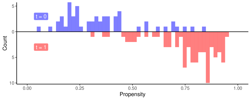
Figure 7: Propensity scores by treatment arm, estimated via probit BART, where $t=0$ corresponds to the control group.

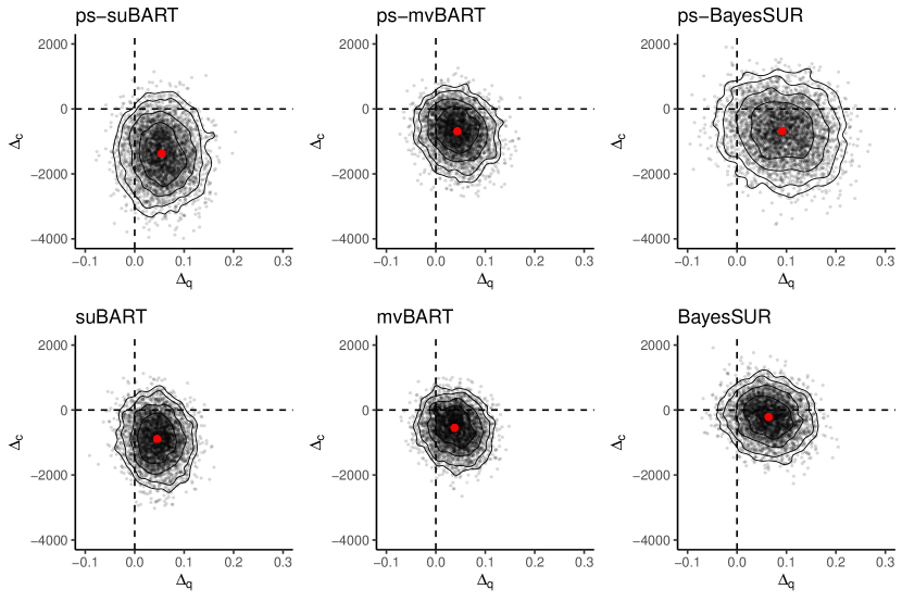
Figure 8: CEPs showing highest density regions of kernel density estimates of the posterior distributions of $\Delta_{c}$ and $\Delta_{q}$ according to each model, with and without propensity scores. The posterior means are indicated by a red dot in each case, the individual draws of $\Delta_{c}$ and $\Delta_{q}$ are shown via grey points, and the contour lines correspond to probability levels of $0.5$, $0.75$, $0.9$, and $0.95$.

In Table 5, we provide summary statistics for $\Delta_{c}$, $\Delta_{q}$, and the INB at a representative value of $\lambda=20000$. We stress that this quantity is not indicative of the cost of the TTCM intervention, which averages €272 per patient (Wiertsema et al., 2019). Rather, this value is indicative of a situation in which decision-makers would be willing to pay €20,000 per additional unit of healthcare-related quality of life, which is much greater as the treatment effect of $\Delta_{q}$ is near-zero. In any case, €20,000 is a commonly used threshold for determining whether an intervention represents value for money in the CEA literature (see e.g., Drummond et al. (2015) and Gabrio et al. (2019). At this chosen $\lambda$ value, we see some considerable differences between ps-suBART and the other methods. This suggests that there may be strong non-linear functional relationships between the covariates and the outcomes (such that suBART benefits from relaxing the linearity assumption of BayesSUR, without requiring pre-specification of the functional forms) and that those relationships may differ for the two outcomes $c$ and $q$ (such that suBART benefits from relaxing the mvBART assumption of a common tree structure). Notably, the estimated treatment effects are markedly smaller in absolute value for each method when propensity scores are excluded and only ps-suBART yields a $95\%$ CI for $\text{INB}_{20000}$ which excludes zero.

Table 5: Posterior means with 95% credible intervals for $\Delta_{c}$, $\Delta_{q}$, and $\text{INB}_{\lambda}$ at a representative value of $\lambda=20000$ for each model, with and without the propensity scores.

Model	Mean and 95% CI
	$\Delta_{c}$		$\Delta_{q}$		$\text{INB}_{20000}$
ps-suBART	$-1371$	$[-2895,189]$	$0.054$	$[-0.020,0.127]$	$2449$	$[210,4635]$
suBART	$-880$	$[-2126,345]$	$0.045$	$[-0.019,0.110]$	$1776$	$[-65,3585]$
ps-mvBART	$-674$	$[-1859,362]$	$0.042$	$[-0.025,0.112]$	$1516$	$[-282,3415]$
mvBART	$-587$	$[-1678,477]$	$0.038$	$[-0.024,0.104]$	$1353$	$[-373,3137]$
ps-BayesSUR	$-698$	$[-2166,771]$	$0.093$	$[-0.012,0.203]$	$2560$	$[-228,5395]$
BayesSUR	$-191$	$[-1285,916]$	$0.063$	$[-0.016,0.144]$	$1448$	$[-660,3556]$

Rather than relying on a single $\lambda$ value, we also show the probability of cost-effectiveness as a function of the willingness-to-pay $\lambda$ in Figure 9. This plot, called a cost-effectiveness acceptability curve (CEAC; Löthgren and Zethraeus, 2000), is a highly-important tool in guiding the decision of which medical intervention to implement. These probabilities are simply estimated by counting all posterior draws for which $\text{INB}_{\lambda}>0$ and dividing this count by the total number of posterior draws. We see some remarkable differences, depending on which method is used for estimation and whether or not the estimated propensity scores are incorporated. Notably, the estimated probability of cost-effectiveness only exceeds the typical $95\%$ reference level at any $\lambda$ under ps-suBART, suBART, and ps-BayesSUR. Moreover, this probability is consistently larger at all $\lambda$ values for all methods when propensity scores are included. Given that we have reason to believe that ps-suBART, ps-mvBART, and ps-BayesSUR are more accurate than their counterparts, we henceforth discuss only these methods.

A particularly striking aspect of Figure 9 is that ps-suBART is the only method for which the estimated probability of cost-effectiveness is well above $95\%$ for all $\lambda$ values. This threshold is typically regarded as a reasonably high probability of cost-effectiveness, so we would be quite content in asserting that the TTCM is cost-effective, regardless of the value of $\lambda$. In fact, even if decision-makers are unwilling to pay anything (i.e., $\lambda=0$) per unit of effect gained, ps-suBART still reports a probability of $0.97$ of being cost-effective compared to regular care. For ps-BayesSUR, the probabilities are notably lower for small $\lambda$ values, even when including propensity scores. Based on the ps-BayesSUR results, we likely would want to collect more data before committing to a final decision. At higher $\lambda$, the probabilities of cost-effectiveness approach the estimates obtained by ps-suBART. For ps-mvBART, the probabilities follow a similar pattern as the ps-suBART estimates, but remain lower across the full range of $\lambda$ values and never reach the $0.95$ reference level. We are thus lead to a substantially different conclusion, depending on the method used: ps-suBART finds strong evidence for TTCM being cost-effective, while the results from the other two models are less conclusive. As previously alluded to, the results for each method are even less conclusive when the propensity scores are omitted from the set of predictors.

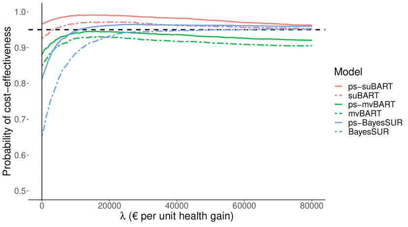
Figure 9: CEACs showing probabilities of cost-effectiveness as a function of $\lambda$ for each model, with and without propensity scores, with a horizontal dotted line at the $0.95$ reference level.

7 Discussion

In this paper, we introduce the suBART model for multivariate outcomes both as means of accounting for non-linearities and interactions in the seemingly unrelated regression framework and as a means of addressing the key limitation of existing multivariate BART approaches which assume a single set of trees, such that the entire response vector is partitioned in the same way by the splitting rules in the ensemble. By modelling each component of the outcome using a univariate BART, suBART captures non-linearities in the relationship between the response and predictors while allowing for and detecting the different subsets of covariates — along with the interactions between them — associated with each response without enforcing common tree structures. We further develop the model to handle multivariate binary outcomes.

The effectiveness of suBART is demonstrated through extensive simulation studies, in which it is shown that the model adequately captures non-linear responses, accurately estimates the covariance structure for multivariate responses, and generally outperforms its main competitors — including other tree-based alternatives and the Bayesian linear SUR — from the points of view of both predictive accuracy and uncertainty calibration. In particular, the extensive evaluation through simulation show that the model exhibits enhanced flexibility compared to its direct multivariate counterpart, mvBART. This flexibility stems from suBART permitting variation in splitting rules across each response, by allowing the trees for each outcome component to differ rather than imposing common tree structures. This enables a more accurate representation, especially when different outcome components depend on distinct sets of predictors.

The main focus of the paper is the application of suBART within the context of cost-effectiveness analysis, a setting in healthcare where it is of interest to jointly estimate the healthcare costs and the health-related quality of life associated with two or more treatment options. In our analysis, we found remarkable differences in results, depending on which regression method we used. It is of course expected to see large differences between linear SUR and the two BART-based models, given the very different model assumptions. The even larger differences between suBART and mvBART are arguably more interesting. To reiterate, suBART assigns each outcome its own tree ensemble, while the trees for all outcomes are the same for mvBART. The large differences in results suggest to us that the assumption of a shared tree structure is a significant one, which may have a strong impact on the results. Unlike mvBART, suBART can accommodate data where the dependence on $\mathbf{X}$ is very different for different components of the outcome vector. In the CEA context, this applies particularly in situations where factors which govern the costs are unrelated to the quality of life, and vice versa. Such situations do occur in practise; for example, when investigating the effect of total knee replacement, Dakin et al. (2012) found that the patients’ sex was a strong predictor of healthcare costs yet had no measurable relationship with quality of life, while the exact opposite was true for the patients’ age. On the other hand, a shared tree structure may lead to estimates which are more precise, without necessarily being more accurate, since there are more data available to inform the tree structure. Um et al. (2023) claim this as an advantage of their method. We do indeed see somewhat smaller posterior variance in the mvBART estimates. We also found that suBART further benefits from the inclusion of estimated propensity scores as an additional predictor. We hence consider what we called ps-suBART to be a natural adaptation of the univariate ps-BART approach and expect it to be a very useful tool in the analysis of observational cost-effectiveness data.

Despite the extensive array of comparisons and scenarios and the additional insights gleaned by suBART in the CEA setting, there remains ample opportunity for further exploration of various extensions to suBART. We delineate some of these possibilities below in light of limitations identified in the simulation studies and real data application.

• Although suBART models non-linear responses with considerable flexibility, the model may still lack the desirable smoothness in certain scenarios; as it is based on the standard BART model, its construction relies on sums of piecewise-constant functions. However, several methods have been proposed to address the inherent lack of smoothness in BART (Linero and Yang, 2018; Prado et al., 2021; Maia et al., 2024) and these approaches could potentially be adapted to suBART as well.

• The suBART framework can be contrasted with the traditional SUR framework in that the conditional expectations are all modelled either via nonparametric univariate BART models or via parametric linear models. In the simulation studies, suBART’s superiority in capturing non-linear responses was comprehensively demonstrated, although BayesSUR was preferable when the response was generated by a simple linear function. A semi-parametric model in which some outcomes are modelled by BART and some are modelled by linear regressions could be of interest in cases where practitioners have strong prior belief about the complexity or lack thereof of one or more responses. Alternatively, such scenarios could be handled by varying the number of trees assigned to each component, though further experiments will be required to verify this.

• In the classic SUR model context, accounting for heteroscedasticity has been a common challenge in the literature (Afolayan and Adeleke, 2018). As suBART represents an effective alternative to the traditional linear SUR, the extension proposed by Pratola et al. (2020) to accommodate heteroscedasticity within BART could be adapted to the suBART setting to address cases where the homoscedasticity assumption is invalid. However, it is important to note that the approach of Pratola et al. (2020) has yet to be extended beyond scalar variance estimation.

• The proposed suBART accommodates two types of multivariate outcomes: all continuous and all binary. We stress however that this flexibility is exclusive and does not apply to both types simultaneously. Previous works in the literature, such as those by Papageorgiou et al. (2014), Zhang et al. (2015), and Pourmohamad and Lee (2016), have adapted a Bayesian framework for handling responses of mixed type. These approaches could potentially be adapted to the suBART framework, providing greater generalisation of the approach, particularly given that trading off treatment costs against binary outcomes (e.g., cancer remission) is often of interest in other healthcare applications.

• The ps-suBART model we used in our analysis of the TTCM data builds on the ps-BART model (Hahn et al., 2020). Hahn et al. (2020) also propose a another related method, the Bayesian causal forest (BCF). The authors and their discussants found the performance of ps-BART and BCF to be similar overall, with each method improving on the other in some settings. One of the advantages of BCF is the ability to directly specify a prior on the amount of treatment effect heterogeneity, while this prior is left implicit in ps-BART. The drawback of this flexibility is that prior specification is more complex in BCF, and it is harder to find reasonable default choices which are appropriate in a variety of settings. Additionally, the computational demands of BCF are greater than those of standard BART. Both of these issues would become even more challenging in the SUR setting with multivariate outcomes. However, given that a multivariate generalisation of BCF has recently been proposed by McJames et al. (2023), which is analogous to the multivariate generalisation of BART developed by Um et al. (2023), there remains scope for embedding BCF in the seemingly unrelated framework as an alternative multivariate approach for conducting cost-effectiveness analyses.

• CEAs are sometimes conducted with more than two treatment options of interest. Conceptually this is similar to the two-treatments setting presented in the TTCM application. For details, we refer interested readers to Drummond et al. (2015), Section 4.4. The ps-suBART method could be easily extended to settings with more than two treatments, by estimating propensity scores using multinomial probit BART (Kindo et al., 2016). With more than one treatment effect for each outcome, and more than one INB, each corresponding to a pairwise comparison of two treatments, the treatment which has a positive INB in all comparisons would be considered cost-effective.

• When presenting the TTCM data, we noted that the original dataset had missing responses for survey questions related to the outcome variables. We bypassed this by working instead with an artificial complete dataset. Ideally, we would prefer to keep the missing values and incorporate the imputation directly into the posterior computation, in order to get coherent estimates of posterior uncertainty. Assuming that the observations are missing at random (the probability of missingness does not depend on the true values of the missing observations, conditional on the observed data), it is straightforward to incorporate imputation into our Gibbs sampler: we would simply draw the missing $y^{(j)}_{i}$ values from their conditional distribution, given in Equation (9). Imputing outcomes with the probit suBART model could be done in a similar manner. However, imputation of missing outcomes for the present application would be further complicated by the fact that the outcomes were calculated after imputing the constituent survey responses by Wiertsema et al. (2019). Imputing missing covariate values, on the other hand, is a totally different matter: our models are formulated conditionally on $\mathbf{X}$, and hence impose none of the distributional assumptions on $\mathbf{X}$ that would be required for imputation tasks. That being said, missing covariate values could be handled by simply adapting the approach of Kapelner and Bleich (2016).

We hope to incorporate these advancements into our forthcoming research plans and anticipate suBART’s adoption in other CEA settings to inspire further developments.

[Acknowledgments] Mateus Maia’s work was supported by Science Foundation Ireland Career Development Award grant number 17/CDA/4695 and SFI research centre award 12/RC/2289P2. Andrew Parnell’s work was supported by: a Science Foundation Ireland Career Development Award (17/CDA/4695); an investigator award (16/IA/4520); a Marine Research Programme funded by the Irish Government, co-financed by the European Regional Development Fund (Grant-Aid Agreement No. PBA/CC/18/01); European Union’s Horizon 2020 research and innovation programme under grant agreement No. 818144; SFI Centre for Research Training 18CRT/6049, and SFI Research Centre awards 16/RC/3872 and 12/RC/2289P2.

We also thank the authors of Wiertsema et al. (2019) for making part of the TTCM data available to us, and allowing us to present the results of our analysis in this paper.

Appendix

Performance evaluation on simulation experiments

In order to evaluate the performance of suBART against its competitors, we conducted experiments replicating those outlined in Section 5, where we varied $n_{\text{train}}=n_{\text{test}}=\{250,500,1000\}$ and $d=\{2,3\}$. This appendix summarises the remaining results omitted from the main paper. The findings illustrated in the boxplots below align with the conclusions drawn in Section 5. Overall, suBART exhibits reasonable performance metrics for both continuous and binary outcome scenarios, either matching or surpassing its tree-based model counterparts. Notably, suBART outperforms the Bayesian linear SUR across all scenarios, with the exception of the responses where the response with the predictors is exclusively linear. Additionally, we provide a summary of the estimation of correlation parameters through tables displaying the RMSE and 50% CI coverage for all $\rho_{kj}$ where $j\neq k$. Across all scenarios, suBART consistently approaches the true values and provides credible intervals with proper coverage ratios.

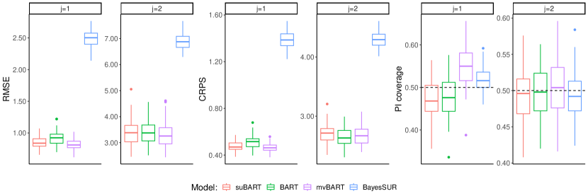
Figure 10: Simulation results for continuous outcomes for Friedman #1 with $n_{\text{train}}=n_{\text{test}}=250$ and $d=2$.

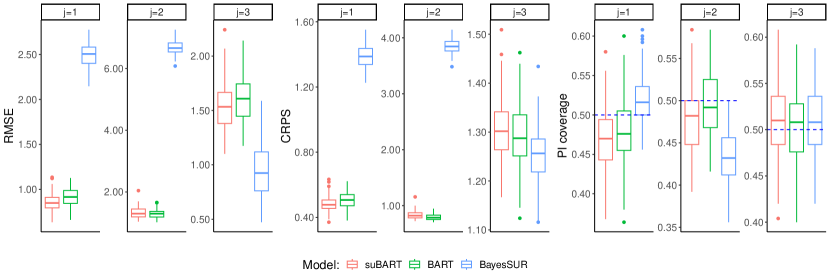
Figure 11: Simulation results for continuous outcomes for Friedman #1 with $n_{\text{train}}=n_{\text{test}}=250$ and $d=3$.

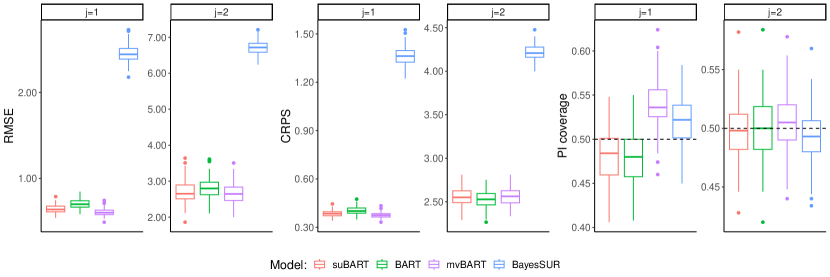
Figure 12: Simulation results for continuous outcomes for Friedman #1 with $n_{\text{train}}=n_{\text{test}}=500$ and $d=2$.

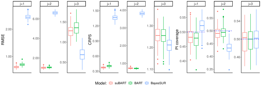
Figure 13: Simulation results for continuous outcomes for Friedman #1 with $n_{\text{train}}=n_{\text{test}}=500$ and $d=3$.

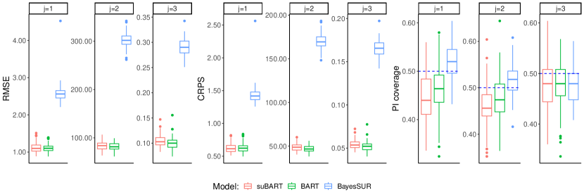
Figure 14: Simulation results for continuous outcomes for Friedman #2 with $n_{\text{train}}=n_{\text{test}}=250$ and $d=2$.

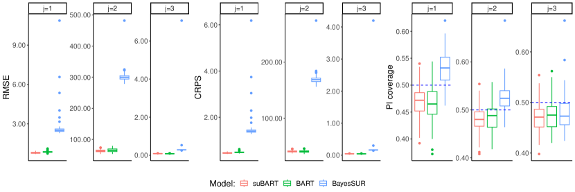
Figure 15: Simulation results for continuous outcomes for Friedman #2 with $n_{\text{train}}=n_{\text{test}}=500$ and $d=2$.

Figure 16: Simulation results for continuous outcomes for Friedman #2 with $n_{\text{train}}=n_{\text{test}}=1000$ and $d=3$.

Figure 17: Simulation results for continuous outcomes for Friedman #2 with $n_{\text{train}}=n_{\text{test}}=500$ and $d=3$.

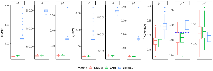
Figure 18: Simulation results for continuous outcomes for Friedman #2 with $n_{\text{train}}=n_{\text{test}}=1000$ and $d=3$.

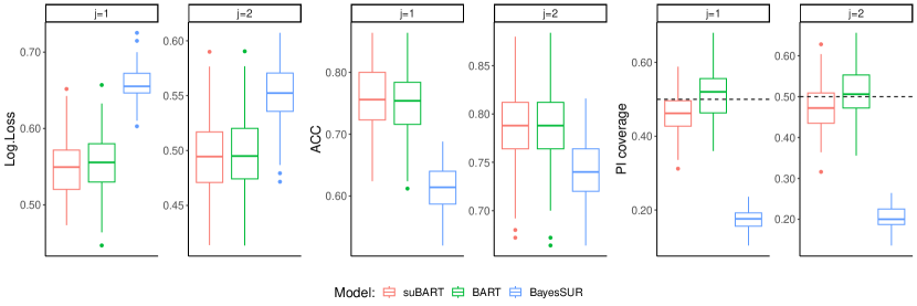
Figure 19: Simulation results for binary outcomes for Friedman #3 with $n_{\text{train}}=n_{\text{test}}=250$ and $d=2$.

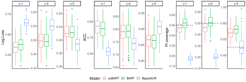
Figure 20: Simulation results for binary outcomes for Friedman #3 with $n_{\text{train}}=n_{\text{test}}=250$ and $d=3$.

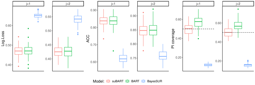
Figure 21: Simulation results for binary outcomes for Friedman #3 with $n_{\text{train}}=n_{\text{test}}=500$ and $d=2$.

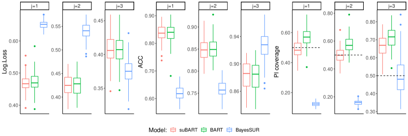
Figure 22: Simulation results for binary outcomes for Friedman #3 with $n_{\text{train}}=n_{\text{test}}=500$ and $d=3$.

Table 6: RMSE and coverage of a 50% CI for $\bar{{\rho}}_{jk}$ from the posterior samples for Friedman #1 with $n_{\text{train}}=n_{\text{test}}=250$ for continuous outcomes.

	RMSE			CI coverage
	suBART	mvBART	BayesSUR	suBART	mvBART	BayesSUR
$d=2$
$\rho_{12}$	$0.05$	$0.09$	$0.34$	$0.33$	$0.17$	$0.00$
$d=3$
$\rho_{12}$	$0.04$	—	$0.39$	$0.30$	—	$0.00$
$\rho_{13}$	$0.07$	—	$0.32$	$0.39$	—	$0.00$
$\rho_{23}$	$0.08$	—	$0.18$	$0.39$	—	$0.02$

Table 7: RMSE coverage of a 50% CI for $\bar{{\rho}}_{jk}$ from the posterior samples for Friedman #1 with $n_{\text{train}}=n_{\text{test}}=500$ for continuous outcomes.

	RMSE			CI coverage
	suBART	mvBART	BayesSUR	suBART	mvBART	BayesSUR
$d=2$
$\rho_{12}$	$0.03$	$0.07$	$0.34$	$0.47$	$0.07$	$0.00$
$d=3$
$\rho_{12}$	$0.02$	—	$0.38$	$0.48$	—	$0.00$
$\rho_{13}$	$0.04$	—	$0.32$	$0.39$	—	$0.00$
$\rho_{23}$	$0.05$	—	$0.17$	$0.45$	—	$0.00$

Table 8: RMSE and coverage of a 50% CI for $\bar{{\rho}}_{jk}$ from the posterior samples for Friedman #2 with $n_{\text{train}}=n_{\text{test}}=250$ for continuous outcomes.

	RMSE			CI coverage
	suBART	mvBART	BayesSUR	suBART	mvBART	BayesSUR
$d=2$
$\rho_{12}$	$0.05$	$0.258$	$0.34$	$0.33$	$0.00$	$0.00$
$d=3$
$\rho_{12}$	$0.04$	—	$0.39$	$0.30$	—	$0.00$
$\rho_{13}$	$0.07$	—	$0.32$	$0.39$	—	$0.00$
$\rho_{23}$	$0.08$	—	$0.18$	$0.39$	—	$0.02$

Table 9: RMSE and coverage of a 50% CI for $\bar{{\rho}}_{jk}$ from the posterior samples for Friedman #2 with $n_{\text{train}}=n_{\text{test}}=500$ for continuous outcomes.

	RMSE			CI coverage
	suBART	mvBART	BayesSUR	suBART	mvBART	BayesSUR
$d=2$
$\rho_{12}$	$0.04$	$0.21$	$0.50$	$0.32$	$0.00$	$0.00$
$d=3$
$\rho_{12}$	$0.05$	—	$0.56$	$0.24$	—	$0.00$
$\rho_{13}$	$0.07$	—	$0.49$	$0.33$	—	$0.01$
$\rho_{23}$	$0.06$	—	$0.71$	$0.55$	—	$0.00$

Table 10: RMSE and coverage of a 50% CI for $\bar{{\rho}}_{jk}$ from the posterior samples for Friedman #2 with $n_{\text{train}}=n_{\text{test}}=1000$ for continuous outcomes.

	RMSE			CI coverage
	suBART	mvBART	BayesSUR	suBART	mvBART	BayesSUR
$d=2$
$\rho_{12}$	$0.06$	$0.17$	$0.49$	$0.02$	$0.00$	$0.00$
$d=3$
$\rho_{12}$	$0.05$	—	$0.58$	$0.02$	—	$0.00$
$\rho_{13}$	$0.05$	—	$0.49$	$0.18$	—	$0.01$
$\rho_{23}$	$0.03$	—	$0.72$	$0.51$	—	$0.00$

Table 11: RMSE and coverage of a 50% CI for $\bar{{\rho}}_{jk}$ from the posterior samples for Friedman #3 with $n_{\text{train}}=n_{\text{test}}=250$ for binary outcomes.

	RMSE		CI coverage
	suBART	BayesSUR	suBART	BayesSUR
$d=2$
$\rho_{12}$	$0.11$	$0.29$	$0.40$	$0.00$
$d=3$
$\rho_{12}$	$0.11$	$0.31$	$0.41$	$0.00$
$\rho_{13}$	$0.11$	$0.11$	$0.53$	$0.21$
$\rho_{23}$	$0.13$	$0.12$	$0.44$	$0.37$

Table 12: RMSE and coverage of a 50% CI for $\bar{{\rho}}_{jk}$ from the posterior samples for Friedman #3 with $n_{\text{train}}=n_{\text{test}}=500$ for binary outcomes.

	RMSE		CI coverage
	suBART	BayesSUR	suBART	BayesSUR
$d=2$
$\rho_{12}$	$0.06$	$0.26$	$0.50$	$0.00$
$d=3$
$\rho_{12}$	$0.05$	$0.28$	$0.50$	$0.00$
$\rho_{13}$	$0.08$	$0.13$	$0.51$	$0.12$
$\rho_{23}$	$0.09$	$0.10$	$0.48$	$0.40$

References

- Afolayan and Adeleke (2018) Afolayan, R. B. and Adeleke, B. L. (2018). “On the efficiency of some estimators for modeling seemingly unrelated regression with heteroscedastic disturbances.” IOSR Journal of Mathematics, 14(4): 1–13.
- Alvarez et al. (2014) Alvarez, I., Niemi, J., and Simpson, M. (2014). “Bayesian inference for a covariance matrix.” In The 26th Annual Conference on Applied Statistics in Agriculture, 71–82. Kansas State University.
- Baio (2012) Baio, G. (2012). Bayesian Methods in Health Economics. Boca Ration, FL, U.S.A.: Chapman & Hall/CRC Biostatistics Series.
- Baldi (2024) Baldi, P. (2024). Probability: An Introduction Through Theory and Exercises. Universitext. Springer Nature.
- Barnard et al. (2000) Barnard, J., McCulloch, R. E., and Meng, X.-L. (2000). “Modeling covariance matrices in terms of standard deviations and correlations, with application to shrinkage.” Statistica Sinica, 1281–1311.
- Breiman (1996) Breiman, L. (1996). “Bagging predictors.” Machine Learning, 24: 123–140.
- Breiman et al. (1984) Breiman, L., Friedman, J. H., Olshen, R. A., and Stone, C. J. (1984). Classification and Regression Trees. New York, NY, U.S.A.: Chapman and Hall/CRC Press, 1 edition. EBook Published 25 October 2017.
- Chakraborty (2016) Chakraborty, S. (2016). “Bayesian additive regression tree for seemingly unrelated regression with automatic tree selection.” In Handbook of Statistics, volume 35, 229–251. Elsevier.
- Chib and Greenberg (1998) Chib, S. and Greenberg, E. (1998). “Analysis of multivariate probit models.” Biometrika, 85(2): 347–361.
- Chipman et al. (1998) Chipman, H. A., George, E. I., and McCulloch, R. E. (1998). “Bayesian CART model search.” Journal of the American Statistical Association, 93(443): 935–948.
- Chipman et al. (2010) — (2010). “BART: Bayesian additive regression trees.” The Annals of Applied Statistics, 4(1): 266–298.
- Clark et al. (2023) Clark, T. E., Huber, F., Koop, G., Marcellino, M., and Pfarrhofer, M. (2023). “Tail forecasting with multivariate Bayesian additive regression trees.” International Economic Review, 64(3): 979–1022.
- Dakin et al. (2012) Dakin, H., Gray, A., Fitzpatrick, R., MacLennan, G., Murray, D., KAT Trial Group, et al. (2012). “Rationing of total knee replacement: a cost-effectiveness analysis on a large trial data set.” BMJ Open, 2(1): e000332.
-
Dorie et al. (2024)
Dorie, V., Chipman, H. A., and McCulloch, R. E. (2024).
dbarts: discrete Bayesian additive regression trees
sampler.
R package version 0.9-26.
URL https://CRAN.R-project.org/package=dbarts - Dorie et al. (2019) Dorie, V., Hill, J. L., Shalit, U., Scott, M., and Cervone, D. (2019). “Automated versus do-it-yourself methods for causal inference: lessons learned from a data analysis competition.” Statistical Science, 34(1): 43–68.
- Drummond et al. (2015) Drummond, M. F., Sculpher, M. J., Claxton, K., Stoddart, G. L., and Torrance, G. W. (2015). Methods for the Economic Evaluation of Health Care Programmes. Oxford, UK: Oxford University Press, 4th edition.
- El Alili et al. (2022) El Alili, M., van Dongen, J. M., Esser, J. L., Heymans, M. W., van Tulder, M. W., and Bosmans, J. E. (2022). “A scoping review of statistical methods for trial-based economic evaluations: the current state of play.” Health Economics, 31(12): 2680–2699.
- Friedman (1991) Friedman, J. H. (1991). “Multivariate adaptive regression splines.” The Annals of Statistics, 19(1): 1–67.
- Friedman (2001) — (2001). “Greedy function approximation: a gradient boosting machine.” The Annals of Statistics, 1189–1232.
- Gabrio et al. (2019) Gabrio, A., Baio, G., and Manca, A. (2019). “Bayesian statistical economic evaluation methods for health technology assessment.” In Hamilton, J. (ed.), Economic Theory and Mathematical Models. Oxford, UK: Oxford Research Encyclopedia of Economics and Finance.
- Gneiting and Raftery (2007) Gneiting, T. and Raftery, A. E. (2007). “Strictly proper scoring rules, prediction, and estimation.” Journal of the American Statistical Association, 102(477): 359–378.
- Hahn et al. (2020) Hahn, P. R., Murray, J. S., and Carvalho, C. M. (2020). “Bayesian regression tree models for causal inference: regularization, confounding, and heterogeneous effects (with discussion).” Bayesian Analysis, 15(3): 965–1056.
- Hastie and Tibshirani (2000) Hastie, T. J. and Tibshirani, R. (2000). “Bayesian backfitting (with comments and a rejoinder by the authors.” Statistical Science, 15(3): 196–223.
- Hernán and Robins (2024) Hernán, M. A. and Robins, J. M. (2024). Causal Inference: What If. Boca Raton, FL, U.S.A.: Chapman & Hall/CRC Press.
- Hill (2011) Hill, J. L. (2011). “Bayesian nonparametric modeling for causal inference.” Journal of Computational and Graphical Statistics, 20(1): 217–240.
- Hoff (2009) Hoff, P. D. (2009). A First Course in Bayesian Statistical Methods, volume 580 of Springer Texts in Statistics. New York, NY, U.S.A.: Springer.
- Huang and Wand (2013) Huang, A. and Wand, M. P. (2013). “Simple marginally noninformative prior distributions for covariance matrices.” Bayesian Analysis, 8(2): 439–452.
- Huber and Rossini (2022) Huber, F. and Rossini, L. (2022). “Inference in Bayesian additive vector autoregressive tree models.” The Annals of Applied Statistics, 16(1): 104–123.
- Imbens and Rubin (2015) Imbens, G. W. and Rubin, D. B. (2015). Causal Inference for Statistics, Social, and Biomedical Sciences: An Introduction. New York, NY, U.S.A.: Cambridge University Press.
- Janizadeh et al. (2021) Janizadeh, S., Vafakhah, M., Kapelan, Z., and Dinan, N. M. (2021). “Novel Bayesian additive regression tree methodology for flood susceptibility modeling.” Water Resources Management, 35: 4621–4646.
- Kapelner and Bleich (2016) Kapelner, A. and Bleich, J. (2016). “bartMachine: machine learning with Bayesian additive regression trees.” Journal of Statistical Software, 70(i04): 1–40.
- Kindo et al. (2016) Kindo, B. P., Wang, H., and Peña, E. A. (2016). “Multinomial probit Bayesian additive regression trees.” Stat, 5(1): 119–131.
- Lamers et al. (2006) Lamers, L. M., McDonnell, J., Stalmeier, P. F. M., Krabbe, P. F. M., and Busschbach, J. J. V. (2006). “The Dutch tariff: results and arguments for an effective design for national EQ-5D valuation studies.” Health Economics, 15(10): 1121–1132.
- Li et al. (2023) Li, F., Ding, P., and Mealli, F. (2023). “Bayesian causal inference: a critical review.” Philosophical Transactions of the Royal Society A, 381(2247): 20220153.
- Linero and Yang (2018) Linero, A. R. and Yang, Y. (2018). “Bayesian regression tree ensembles that adapt to smoothness and sparsity.” Journal of the Royal Statistical Society Series B: Statistical Methodology, 80(5): 1087–1110.
- Löthgren and Zethraeus (2000) Löthgren, M. and Zethraeus, N. (2000). “Definition, interpretation and calculation of cost-effectiveness acceptability curves.” Health Economics, 9(7): 623–630.
- Maia et al. (2024) Maia, M., Murphy, K., and Parnell, A. C. (2024). “GP-BART: a novel Bayesian additive regression trees approach using Gaussian processes.” Computational Statistics & Data Analysis, 190: 107858.
- McJames et al. (2023) McJames, N., Parnell, A. C., Goh, Y. C., and O’Shea, A. (2023). “Bayesian causal forests for multivariate outcomes: application to Irish data from an international large scale education assessment.”
- Papageorgiou et al. (2014) Papageorgiou, G., Richardson, S. T., and Best, N. (2014). “Bayesian non-parametric models for spatially indexed data of mixed type.” Journal of the Royal Statistical Society Series B: Statistical Methodology, 77(5): 973–999.
- Peruzzi and Dunson (2022) Peruzzi, M. and Dunson, D. B. (2022). “Spatial multivariate trees for big data Bayesian regression.” The Journal of Machine Learning Research, 23(1): 747–786.
- Pourmohamad and Lee (2016) Pourmohamad, T. and Lee, H. K. H. (2016). “Multivariate stochastic process models for correlated responses of mixed type.” Bayesian Analysis, 11(3): 797 – 820.
- Prado et al. (2021) Prado, E. B., Moral, R. A., and Parnell, A. C. (2021). “Bayesian additive regression trees with model trees.” Statistics and Computing, 31(20): 1–13.
- Pratola et al. (2020) Pratola, M. T., Chipman, H. A., George, E. I., and McCulloch, R. E. (2020). “Heteroscedastic BART via multiplicative regression trees.” Journal of Computational and Graphical Statistics, 29(2): 405–417.
- Ramful and Zhao (2009) Ramful, P. and Zhao, X. (2009). “Participation in marijuana, cocaine and heroin consumption in Australia: a multivariate probit approach.” Applied Economics, 41(4): 481–496.
- Robert (1995) Robert, C. P. (1995). “Simulation of truncated normal variables.” Statistics and Computing, 5: 121–125.
- Rocková (2020) Rocková, V. (2020). “On semi-parametric inference for BART.” In International Conference on Machine Learning, 8137–8146. PMLR.
- Ročková and Saha (2019) Ročková, V. and Saha, E. (2019). “On theory for BART.” In The 22nd International Conference on Artificial Intelligence and Statistics, 2839–2848. PMLR.
- Rocková et al. (2020) Rocková, V., Van der Pas, S., et al. (2020). “Posterior concentration for Bayesian regression trees and forests.” Annals of Statistics, 48(4): 2108–2131.
- Rudolph et al. (2023) Rudolph, K. E., Williams, N. T., Miles, C. H., Antonelli, J., and Diaz, I. (2023). “All models are wrong, but which are useful? Comparing parametric and nonparametric estimation of causal effects in finite samples.” Journal of Causal Inference, 11(1): 20230022.
- Sarti et al. (2023) Sarti, D. A., Prado, E. B., Inglis, A. N., Dos Santos, A. A., Hurley, C. B., Moral, R. A., and Parnell, A. C. (2023). “Bayesian additive regression trees for genotype by environment interaction models.” The Annals of Applied Statistics, 17(3): 1936–1957.
-
Stan Development Team (2024a)
Stan Development Team (2024a).
“RStan: the R interface to Stan.”
R package version 2.32.5.
URL https://mc-stan.org/ -
Stan Development Team (2024b)
— (2024b).
Stan User’s Guide.
Stan Development Team.
URL https://mc-stan.org/docs/ - Um et al. (2023) Um, S., Linero, A. R., Sinha, D., and Bandyopadhyay, D. (2023). “Bayesian additive regression trees for multivariate skewed responses.” Statistics in Medicine, 42(3): 246–263.
- Vink et al. (2014) Vink, G., Frank, L. E., Pannekoek, J., and Van Buuren, S. (2014). “Predictive mean matching imputation of semicontinuous variables.” Statistica Neerlandica, 68(1): 61–90.
- Wand et al. (2011) Wand, M. P., Ormerod, J. T., Padoan, S. A., and Frühwirth, R. (2011). “Mean field variational Bayes for elaborate distributions.” Bayesian Analysis, 6(4): 847–900.
- Wiertsema et al. (2019) Wiertsema, S. H., Van Dongen, J. M., Geleijn, E., Huijsmans, R. J., Bloemers, F. W., De Groot, V., and Ostelo, R. W. J. G. (2019). “Cost-effectiveness of the transmural trauma care model (TTCM) for the rehabilitation of trauma patients.” International Journal of Technology Assessment in Health Care, 35(4): 307–316.
- Willan et al. (2004) Willan, A. R., Briggs, A. H., and Hoch, J. S. (2004). “Regression methods for covariate adjustment and subgroup analysis for non-censored cost-effectiveness data.” Health Economics, 13(5): 461–475.
- Yee and Deshpande (2023) Yee, R. and Deshpande, S. K. (2023). “Evaluating plate discipline in Major League Baseball with Bayesian additive regression trees.” Journal of Quantitative Analysis in Sports. Advanced online publication.
- Zellner (1962) Zellner, A. (1962). “An efficient method of estimating seemingly unrelated regressions and tests for aggregation bias.” Journal of the American Statistical Association, 57(298): 348–368.
- Zhang (2020) Zhang, X. (2020). “Parameter-expanded data augmentation for analyzing correlated binary data using multivariate probit models.” Statistics in Medicine, 39(25): 3637–3652.
- Zhang et al. (2006) Zhang, X., Boscardin, W. J., and Belin, T. R. (2006). “Sampling correlation matrices in Bayesian models with correlated latent variables.” Journal of Computational and Graphical Statistics, 15(4): 880–896.
- Zhang et al. (2015) Zhang, X., Boscardin, W. J., Belin, T. R., Wan, X., He, Y., and Zhang, K. (2015). “A Bayesian method for analyzing combinations of continuous, ordinal, and nominal categorical data with missing values.” Journal of Multivariate Analysis, 135: 43–58.