CHOSEN: Contrastive Hypothesis Selection for Multi-View Depth Refinement
Abstract
We propose CHOSEN, a simple yet flexible, robust and effective multi-view depth refinement framework. It can be employed in any existing multi-view stereo pipeline, with straightforward generalization capability for different multi-view capture systems such as camera relative positioning and lenses. Given an initial depth estimation, CHOSEN iteratively re-samples and selects the best hypotheses, and automatically adapts to different metric or intrinsic scales determined by the capture system. The key to our approach is the application of contrastive learning in an appropriate solution space and a carefully designed hypothesis feature, based on which positive and negative hypotheses can be effectively distinguished. Integrated in a simple baseline multi-view stereo pipeline, CHOSEN delivers impressive quality in terms of depth and normal accuracy compared to many current deep learning based multi-view stereo pipelines.
1 Introduction
Geometry acquisition through multi-view imagery is a crucial task in 3D computer vision. In the multi-view stereo matching (MVS) framework, image patches or features are matched and triangulated to find 3D points (Collins, 1996; Furukawa & Ponce, 2010). The dense geometry is usually represented as a depth map for each view. Due to view dependent appearance, occlusion and self-similarity in the real world scenarios, the matching signal is often too noisy to directly give accurate and complete geometry. Traditionally, this problem have been attacked by some carefully designed optimization and filtering scheme (Barron & Poole, 2016; Taniai et al., ), directly on the depth map or indirectly inside a matching cost volume, where they impose certain priors on the smoothness of the resulting geometry, making use of the confidence of matching and appearance in a larger spatial context.
With the advancement of deep learning, many research works have combined the ideas with traditional MVS. Early works (Yao et al., 2018, 2019) typically involve extracting convolutional features from the images, building one cost volume (indexed by a sequence monotone depth hypotheses for each pixel), or several in a multi-resolution hierarchy, and transform these cost volumes using 3D convolutions into a ”probability volume” so that depth map can be obtained by taking the expectation
| (1) |
More recent works have more complicated designs regarding cost computation and aggregation (Wang et al., 2021), visibility and uncertainty estimation (Zhang et al., 2023a; Cheng et al., 2020), loss functions (Peng et al., 2022), feature backbones (Cao et al., 2023), feature fusion (Zhang et al., 2023b), and consequently have yielded impressive progress on various benchmarks. However, the evaluation has been limited to point cloud reconstruction, and little attention was paid to, and thus the lack thereof, the raw output’s quality in terms of depth and normal accuracy. Moreover, the fixed training and testing benchmarks also result in limited discussion on the learning and inference task under the variance of the multi-view acquisition setups, including different metric scales, camera relative positioning and lenses (focal lengths). Therefore, for a new capture setup substantially different from the training set, one is usually left with the job of determining what hyper-parameters to choose for cost volumes and probably retrain the model of choice. In fact, both of the problems can be attributed to the approach of using Eq.(1) to obtain depth estimations: depths hypotheses at different pixels, or across different datasets, may not be well aligned. The first results in non-smoothness, and the second results in poor generalization.
In this work, we turn our attention to the problem of learning to refine depth with multi-view images while keeping in mind that they can be from very different setups, and how to best sample hypotheses for depth refinement. We will discuss in Sec.3.1 the proper solution space to perform the learning task, and present an alternative to the approach of Eq.(1) in Sec.3.2. Much as inspired by the PatchMatch (Barnes et al., 2009; Bleyer et al., 2011) methodology, our framework, named CHOSEN, learns to refine the depth by iteratively re-sampling and selecting the best hypotheses, thus eliminating the need of a ”probability volume”.
In the following we identify and underline the core design elements that enable CHOSEN to produce significantly improved depth and normal quality:
-
•
Transformation of the depth hypotheses into a solution space defined by the acquisition setup.
-
•
The use of first order approximation to sample spatial hypotheses to propagate good hypotheses to their neighborhood.
-
•
A carefully designed hypothesis feature so that it’s informative for contrastive learning.
-
•
Each hypothesis is evaluated independently so that the refinement is robust to arbitrary hypothesis samples.
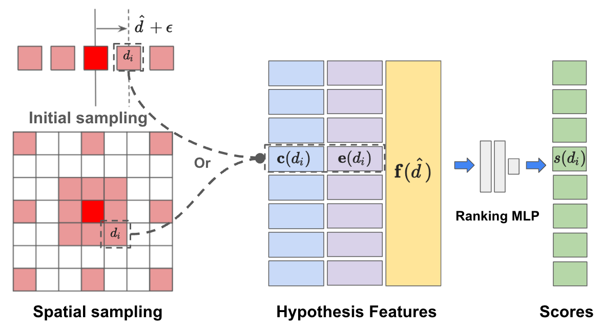
An overview of CHOSEN is illustrated in Fig.1.
To demonstrate the effectiveness of CHOSEN, in Sec.3.3 we describe how we embed it in a minimalist MVS pipeline where the only extra learnable part is the feature extraction using light-weight U-Nets (Ronneberger et al., 2015). We perform comprehensive ablation experiments to justify our design, and compare the quality of our refined depths with various recent deep learning based MVS pipelines. Without bells and whistles, our baseline model is easy to train, fast to converge, and already delivers impressive depth estimation quality.
2 Related work
MVS algorithms are often categorized by the representation used to reconstruct the output scene, e.g. volume (Kutulakos & Seitz, 2000; Kar et al., 2017; Ji et al., 2017), point cloud (Furukawa & Ponce, 2010; Lhuillier & Quan, 2005; Lin et al., 2018; Insafutdinov & Dosovitskiy, 2018), depth map (Galliani et al., 2016; Tola et al., 2012; Schönberger et al., 2016), etc. However, depth map is probably the most flexible and efficient representation among existing ones. While depth map can be considered as a particular case of point cloud representation, (e.g., pixel-wise point), it reduces the reconstruction task to a per-view (2D) depth map estimation. These MVS approaches can be further grouped in hand-crafted (traditional) methods or learning based solutions. Traditional MVS pipelines extend the two-view case (Scharstein & Szeliski, 2002) by introducing a view-selection step that aggregates the cost from multiple images to a given reference view. The view selection can be performed per-camera (Galliani et al., 2015) or per-pixel (Schönberger et al., 2016). These approaches (Galliani et al., 2015, 2016; Tola et al., 2012; Schönberger et al., 2016) then rely on well engineered photometric cost functions (ZNCC, SSD, SAD, etc.) to estimate the scene 3D geometry, by selecting the best depth hypothesis that leads to the lowest aggregated cost. However these cost functions usually perform poorly on texture-less or occluded areas, and under complex lighting environments where photometric consistency is unreliable. Hence further post-processing and propagation steps are used to improve the final estimate (Schönberger et al., 2016; Galliani et al., 2015). We refer readers to (Furukawa & Hernández, 2015) for additional details regarding traditional multi-view stereo pipelines.
Recently, MVS algorithms have showed impressive quality of 3D reconstructions in terms of accuracy and completeness, mostly thanks to the increase popularity of deep learning based solutions (Yao et al., 2018, 2019; Yu & Gao, 2020; Gu et al., 2020; Wang et al., 2021; Zhang et al., 2023b; Cao et al., 2023). These methods often make use of multi-scale feature extractors (Cheng et al., 2020; Tankovich et al., 2021; Chang & Chen, 2018), cost-volumes (Kendall et al., 2017; Khamis et al., 2018; Zhang et al., 2018), and guided refinement (Yao et al., 2018; Pang et al., 2017; Khamis et al., 2018) to retrieve the final 3D estimate. Typically, they leverage U-Nets (Ronneberger et al., 2015) to build a single or a hierarchy of cost volumes with predetermined depth hypotheses. Then, these cost volumes are regularized using 3D convolutions and the final depth map is regressed from the regularized probability volume. However, to achieve high resolution depth accuracy, it requires sampling a large number of depth planes, which is limited by memory consumption.
Researchers are also opening other frontiers in deep learning based MVS. UCS-Net (Cheng et al., 2020) and Vis-MVSNet (Zhang et al., 2023a) use some uncertainty estimate for an adaptive generation of cost volumes. PVSNet (Xu & Tao, 2020) and PatchmatchNet (Wang et al., 2021) learn to predict visibility for each source image. The approach of Eq.(1) is considered critically in (Peng et al., 2022), although it was only considered from the loss function perspective. GeoMVSNet (Zhang et al., 2023b) proposes a geometry fusion mechanism in the MVS pipline. Most recently, transformer based methods (Ding et al., 2022; Cao et al., 2023, 2024) exploits the attention mechanism for more robust matching and context awareness. In particular, MVSFormer (Cao et al., 2023) has combined this approach with the powerful pre-trained DINO features (Oquab et al., 2023).
It is worth mentioning that existing methods usually need to hand-tune hyper-parameters such as the depth range, hypotheses spacing, and number of hypotheses to ensure sufficient and accurate coverage for the new application. Some of these methods adopt 2D convolutional neural networks to obtain final depth estimations, using RGB image to guide depth up-sampling and refinement (Khamis et al., 2018; Hui et al., 2016; Wang et al., 2021). Consequently, these methods often generalize poorly to new camera setups or new scenes.
3 Framework
There are two important aspects in our CHOSEN framework. In Sec.3.1 we discuss how to define a suitable solution space for the depth hypotheses and how to sample them. This has to accommodate the fact that input depths can be of arbitrary scale, and are computed from different multi-view systems. Then in Sec.3.2 we detail our design of a ranking module that is able to process arbitrarily sampled hypotheses, and how it can be trained to effectively and robustly distinguish the good hypotheses from the bad ones.
3.1 Hypothesis representation and sampling
Pseudo disparity representation
We find it crucial to operate in a transformed inverse depth representation, which we call pseudo disparity - akin to disparity for rectified stereo pairs. Denoting the metric depth as , the pseudo disparity writes
| (2) |
where we choose to be the focal length (unit in pixels) of the reference camera, and the metric distance between the reference camera and the closest source camera. The scaling factor converts the inverse depth into the pixel space, and approximates the correct accuracy level of the capture setup in use, granted that the cameras have sufficient frustum overlap and similar focal lengths. This representation not only allows us to build hypothesis feature insensitive to the variance in metric or intrinsic scales, but also defines the correct granularity in the solution space where we distinguish the positive and negative samples for contrastive learning, thus enabling our depth refinement model to learn and infer across various acquisition setups.
Initial hypotheses sampling
The initial depth hypotheses are constructed as a volume where we will look for the optimal hypothesis per pixel that has the lowest matching cost. In case there is no initial depth available, we initialize the volume using uniformly spaced slices in the range , where the number of slices can be chosen so that the slices sit apart from each other, and initialize the depth to be the one with lowest matching cost. We refer to the corresponding cost volume as the full cost volume. In case an previous depth is available, the volume will be restricted to be uniformly spaced in . A cost volume built using this set of hypotheses is referred to as a local cost volume, and will be updated to be the one with lowest matching cost in the local volume. In addition, we apply uniform random perturbation in to each hypothesis at each pixel for both volumes to robustify the training and estimation. Note that there are no other particular restrictions on choices of or as long as the spacing is appropriate and the coverage is sufficient, and in particular they can be changed without re-training.
Spatial hypothesis sampling
Inspired by the PatchMatch framework (Barnes et al., 2009; Bleyer et al., 2011), we use spatial hypotheses to expand good solutions into their vicinity. Specifically, we sample a set of hypotheses for each pixel by collecting the propagated depths from its spatial neighbors. The propagation is facilitated through first order approximation. Denote to be gradient of the depth , be a spatial neighbor of the pixel . The propagated depth from to is defined as
| (3) |
In practice we use a fixed set of ’s for each pixel, though it is more of a convenience than requirement. We conduct sampling and best hypothesis selection in multiple iterations and resolutions.
3.2 Contrastive learning for hypothesis ranking
It is crucial to keep in mind that we don’t assume any structure in the sampled set of hypotheses. In fact, many among them can be wildly bad samples, especially if the initial depth is too noisy. Hence it implies that each hypothesis should be evaluated independently, and our task is to learn to distinguish the good hypotheses from the bad ones.
To achieve our objective, we designate the ranking model to be a small MLP that takes a hypothesis feature and its context feature, and outputs a score for the input hypothesis. Among all the hypotheses at a particular pixel, the one with the highest score will be selected to be the updated depth estimation . The ranking and selection goes on iteratively to refine the depth estimation, where the new will be used to generate better hypotheses with the updated context feature.
Our design for the hypothesis feature and context update mechanism is illustrated in Fig.1. There are three general guidelines we have followed when we design the hypothesis feature: (1) It should inform how well the matching is given by the hypothesis; (2) It should inform how well the hypothesis fits into the current spatial context; (3) It should be robust to different camera setups and resolutions. With these in mind, we propose to use the concatenation of the following three simple quantities computed from a hypothesis :
| (4) |
The first term consists of the matching costs linearly interpolated from the cost volume for a fixed set of perturbations
| (5) |
Note that is defined in the pseudo disparity space.
The second term is a ”tamed” version of the second-order error in the one-ring neighborhood of the pixel . Note that the error is computed against in the pseudo disparity space so that it can work across different metric and intrinsic scales.
| (6) |
Finally, is a learned context feature of the previous refined depth, whose inputs are the concatenation of , and the feature from a U-Net describing the reference view’s high level appearance. We use a two-layer convolution network to initialize , and subsequently we use a convolutional gated recurrent unit (GRU) to update given the updated . We remark that the overall iterative update is similar to the RAFT (Teed & Deng, 2020) framework, with the addition of the geometric error term . We will discuss its crucial contribution in our ablation study in Sec.4.2.
We use a contrastive loss to supervise the ranking module. Let be the ground truth depth and be the set of input hypotheses. We define the positive sample group to be those within -pseudo disparity of the ground truth
| (7) |
Denote the score of to be . Our contrastive loss is defined as
| (8) |
3.3 Baseline MVS design
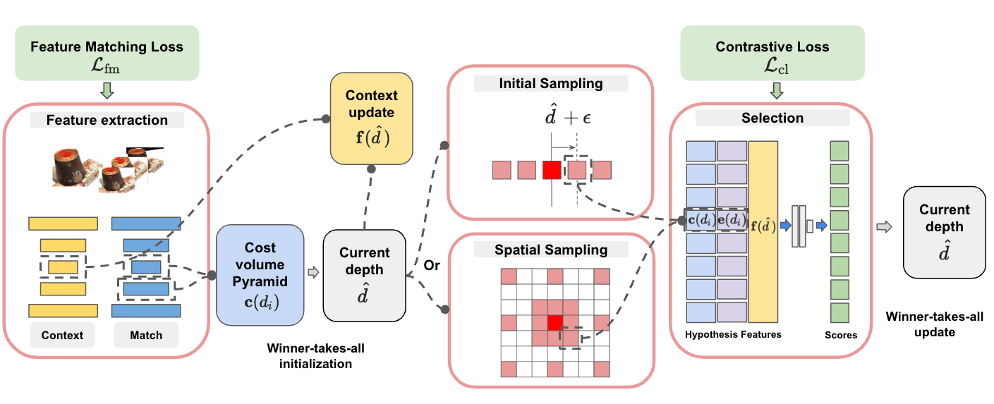
It should be noted that our method can be embedded end-to-end in any deep learning based MVS framework. Here we will demonstrate the design of a simple end-to-end MVS pipeline. We use simple feature correlation as the matching cost, so that there are no learnable components for cost volume filtering, depth refinement, or confidence prediction. The only learnable parts are the ranking MLP, context update convolutional layers, the light-weight U-Nets used for extracting matching feature as well as the high level appearance of the reference view.
Hence our matching component is very noisy, and suboptimal in the cases where there are large view distortion, relative rotation or scale change. One should expect straightforward improvement when additional techniques are incorporated, such as cost volume filtering (Yao et al., 2018), learnable aggregation (Zhang et al., 2023a), other feature extraction backbones (Cao et al., 2023), etc. Even with noisy feature correlation matching signal, we show in Sec.4.3 that it can achieve superior quality in depth and normal compared to many state-of-art MVS works on the DTU dataset, highlighting the robustness of our approach.
Feature extraction
We use a two-stream feature extraction architecture similar to (Teed & Deng, 2020). First, we use a matching feature network extracts distinctive features that are then used to evaluate the cost of depth hypotheses between the reference and other source views. Second, we use a context feature network that learns high-level spatial cues for learnable hypothesis selection, applied only on the reference image. Both networks are based on a light-weight U-Net architecture (Ronneberger et al., 2015) which extracts features from coarse to fine.
Matching cost aggregation
We choose the negative correlation as the matching cost:
| (9) |
where denotes the -th source view feature warped to the reference view through the hypothesis . We aggregate the costs from all source views to have a single cost volume simply as
| (10) |
where
| (11) |
computes the weighting for each view and hypothesis, and is chosen so that it downplays the contribution from higher cost, increases the importance of lower cost, and not sensitive if the cost is close to , thanks to the cubic exponent.
Cost volume pyramid
As an optional benefit, we observe that it’s possible to compute the matching costs for lower resolution depth using higher resolution feature. Specifically, we construct a grid , indexed by lower resolution pixels, which samples the corresponding locations in the higher resolution feature. We can then compute the warped pixel location and the matching costs using the camera intrinsics and features corresponding to the higher resolution.
In practice, we typically compute one additional cost volume using higher resolution features. The new hypotheses are centered around the hypothesis of lowest cost in the coarse cost volume, spaced according the scale defined by the higher resolution pseudo disparity space. These two cost volumes now form a cost volume pyramid, which will be used to provide both coarse and fine matching information to the our ranking module through in Eq.(5). We will demonstrate in Sec.4.2 that using the higher resolution feature can unblock a higher level of accuracy even at lower resolution output, but it’s otherwise not crucial to the success of our hypothesis ranking module.
Overall pipeline
Our baseline MVS pipeline, as depicted in Figure 2, starts by extracting features from a reference view and multiple source views. The first depth estimation is obtained as the lowest cost hypothesis from the full cost volume. A cost volume pyramid is then constructed around the previous depth estimation. The refinement is performed on a hierarchy of resolutions. The refined depth from lower resolution will be upsampled using nearest-neighbor and set to be the initial depth for the next higher resolution.
Training
Similar to the contrastive loss used in (Tankovich et al., 2021), we supervise the feature matching using a simple contrastive loss
| (12) |
where is the ground truth depth, and is the negative sample that is at least -pseudo disparity away from the ground truth and has the lowest matching cost
| (13) |
The loss will not penalize cost of already lower than or higher than . We choose in lower resolution and for all resolution, so that the learned features will be as distinctive as possible. We found it better to choose a lower in higher resolution (e.g. 0.8) due to the frequent appearance of local texture-less regions. Note that there is no any kind of cost volume regularization. Furthermore, we enforce the matching feature network to be only trained by the above loss, meaning it will not be influenced by the depth refinement. Therefore, the total loss of this baseline model is simply
| (14) |
where only updates the matching feature U-Net, and updates the context feature U-Net in the reference view, the ranking MLP and the convolutional layers that initialize and update in Eq.(4).
4 Experiments
| Method | mm | MAE(@mm) | (@mm) | (@mm) |
| baseline: (,,)-(,,1) | ||||
| baseline: (,,)-(,,1) + BlendedMVS | ||||
| \hdashlinebaseline: (,,)-(,,1) | ||||
| baseline: (,,)-n.a. | ||||
| \hdashlinebaseline w/o selection: (,,)-(,,1) | ||||
| \hdashlinebaseline w/o term: (,,)-(,,1) | ||||
| \hdashlinebaseline w/o CHOSEN: (,,)-(,,1) | ||||
| MVSFormer (Cao et al., 2023) | ||||
| GeoMVSNet (Zhang et al., 2023b) | ||||
| GBi-Net (Mi et al., 2022) | ||||
| IterMVS (Wang et al., 2022) | ||||
| PatchMatchNet (Wang et al., 2021) | ||||
| UCSNet (Gu et al., 2020) |
4.1 Implementation details
We evaluate our depth refinement method using the baseline MVS pipeline described in Sec.3.3. Typically, we extract matching features at , , and of the original resolution, and context features at and of the original resolution. The depth is initialized by winner-take-all from the full cost volume at resolution that has slices, and a cost volume pyramid is built on resolution matching features. One refinement stage consists of 4 iterations, where twice on initial sampled hypotheses and twice on spatially sampled hypotheses, in an alternating fashion. After upsampling the refined depth using nearest neighbor, we repeat the same refinement stage at resolution, with a pyramid. Finally, the last refinement stage is performed with a pyramid with output at resolution. Each refinement stage has their own parameters for the ranking MLP and context update networks. We denote this default configuration as . Different choices for cost volume pyramid configurations and their effects will be discussed in Sec 4.2.
We set in the initial hypotheses sampling, giving hypotheses. For spatial sampling, we use a set of offsets consists of dilated regular patches with dilation rate of and , without repeating the patch center, giving in total hypotheses for each pixel. This offset configuration is the same as the one illustrated in the spatial sampling part of Fig.1.
The model is trained and tested on a single NVIDIA A100 GPU (40G). We first train with batch size 4, at input resolution , up to 200k iterations using the default Adam optimizer (Kingma & Ba, 2014) at a learning rate of . We then fine-tune for up to 50k iterations at input resolution at a learning rate of . During training, we fix the closest source view and randomly sample two from the remaining source views, which is the only data augmentation we used. For testing, it takes around seconds to run at with source views. We provide results both from models trained on DTU (Jensen et al., 2014) training set only, and on DTU mixed with the BlendedMVS (Yao et al., 2020) dataset, which will be tagged specifically.
Depth & normal metrics
We use the following metrics to measure the quality of depth and its induced normal map on the DTU evaluation dataset:
-
•
mm: the percentage of pixels that have less than -mm of absolute error.
-
•
MAE(@mm): the mean absolute error on pixels that have less than -mm of absolute error.
-
•
(@mm): the percentage of pixels where the normal is within of angular error out of all pixels whose absolute error is less than -mm.
The ground truth depth are resized to the same resolution of the outputs using nearest neighbor. The normals are computed from the 3D coordinate’s gradients using the Sobel filter. All the above metrics are computed only on the valid pixels where the ground-truth is available.
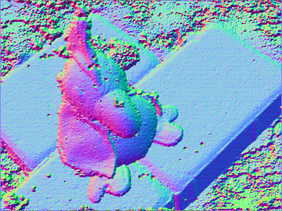
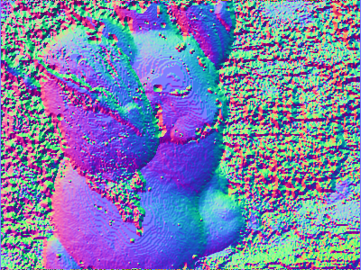
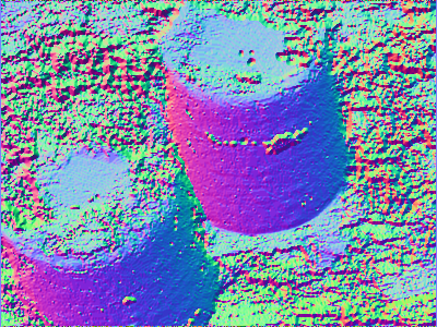
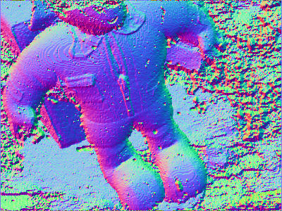
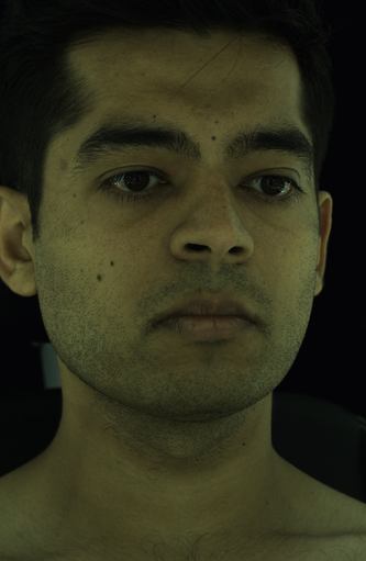
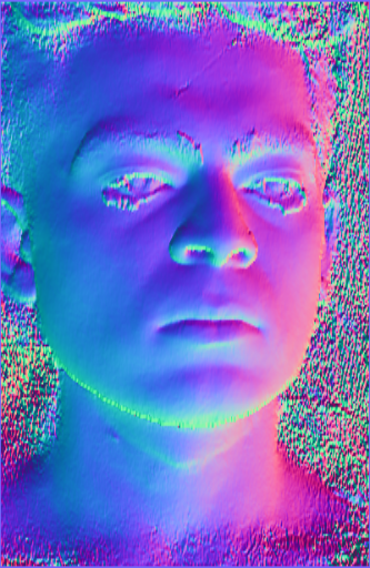
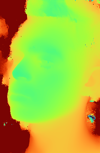
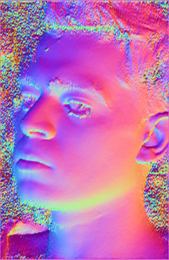
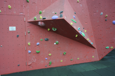
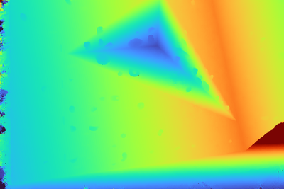
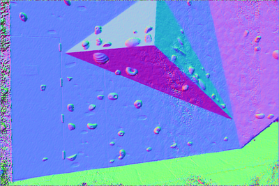
Color image


Ground truth
Ours
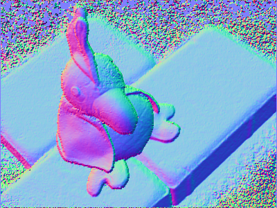
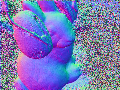
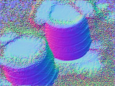
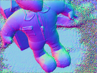
MVSFormer
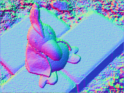
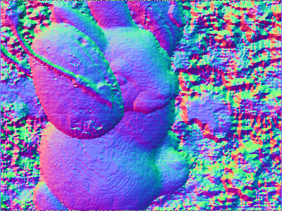
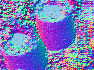
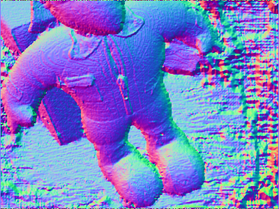
GeoMVSNet
GBi-Net


4.2 Ablation studies
Cost volume pyramid design
Here we study the effects of different cost volume pyramid configurations. We choose the following variants of the configuration:
-
•
(,,)-(,,): There are 3 stages of refinement with , and cost volume pyramids, and output refined depth at resolution. This is our default configuration and we also include the results trained on data mixed BlendedMVS.
-
•
(,,)-(,,): There are 3 stages of refinement with , and cost volume pyramids, and output refined depth at resolution.
-
•
(,,)-n.a: Only the coarsest resolution matching feature is used. There are 3 stages of refinement with resolution feature, and output refined depth at resolution.
Quantitative results on DTU testing set are reported in the first four rows in Tab.1. First of all, notice that even without cost volume pyramid, our method performs reasonably well, indicating that the pyramid design mainly unblocks higher accuracy at lower resolution output, but otherwise is an optional feature. Second, we can observe from the first and third rows in Tab.1 that the mm metrics are similar for the outputs at resolution and resolution, so long as the full resolution matching features are used. Comparing (third and fourth rows) and (first and second rows) output resolution, we can observe that it becomes more difficult to get accurate normals at higher resolution. This is due to the fact that high frequency details only emerge in higher resolution, which may be impossible to obtain without a photometric appearance model. Lastly, we remark that the worse results from mixed data training is likely due to that BlendedMVS contains images with severe aliasing artifacts, which could hurt our model training with .
Selection v.s. expectation
The ability to rank arbitrary hypotheses is essential to the success of our depth refinement. Here we illustrate the point by comparing with an approach where the learned score for each hypothesis is used for taking a weighted average. In this ablated approach, the refined depth is obtained by
and we use smoothed loss between and in place of . Everything else in the pipeline stays the same. Quantitative results are reported in the fifth row of Tab.1. We note that this alternative approach based on weighted average is much less accurate than the our approach based on ranking and selection. This can be attributed to the difficult task of learning the weights for arbitrary hypotheses, while learning to classify the hypotheses is a much easier task.
Hypothesis feature design
The ”tamed” second order error term in Eq.(4) can be viewed as an extra component compared to the input feature design in the RAFT (Teed & Deng, 2020) framework for optical flow estimation. Here we show that it is a vital component in the hypothesis ranking model that improves the overall smoothness and accuracy. Quantitative results on DTU testing set are reported in the sixth row of Tab.1. Since each hypothesis is evaluated independently, without the information about how well a particular hypothesis fits in the local geometry, the model struggles to select the best hypothesis solely based on matching and context information.
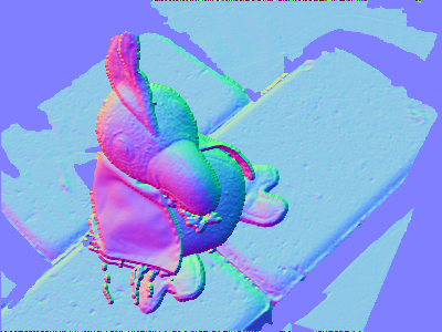
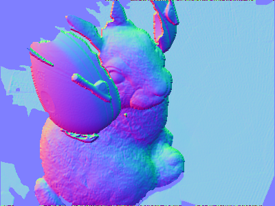
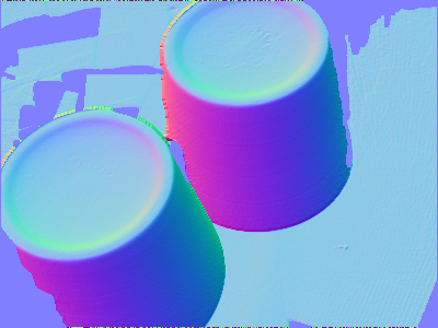
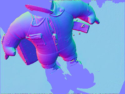
4.3 Comparisons on depths and normals
We collect the testing results from various recent deep learning based MVS works in the last part of Tab.1. The outputs for the candidate models and ground truths are resized to of input resolution using nearest neighbor. Our simple baseline MVS pipeline significantly outperforms the strongest state-of-art in terms depth and normal quality. Visual comparisons are shown in Fig.3.
4.4 Qualitative results
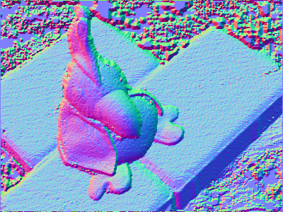
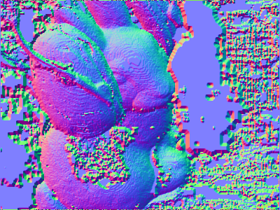
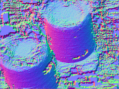
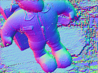
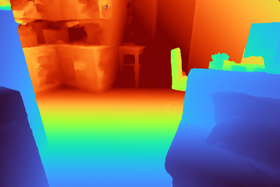
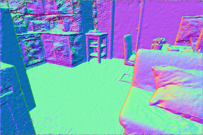
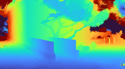
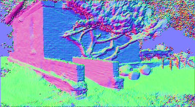
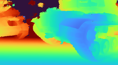
We demonstrate the excellent generalization ability of our simple baseline on various datasets including MultiFace (Wuu et al., 2022), Tanks & Temples (Knapitsch et al., 2017) and ETH3D (Schops et al., 2017). Results in Fig.4 use the same baseline model trained on mixture of DTU and BlendedMVS reported in Tab.1.
5 Limitations and Conclusion
One limitation of CHOSEN is that it becomes more expensive to sample and select from a large number of hypotheses at high resolution. This is part of the reason why we settled at resolution to arrive at a sweet spot of both performance and run time. Another limitation is that we did not focus on bundle adjustment and joint filtering of depths for point cloud and surface reconstruction, which we believe should be a subject of its own interests, especially considering the proliferation of volumetric based methods such as (Zhang et al., 2021).
We have demonstrated that CHOSEN is simple yet effective for multi-view depth refinement. It iteratively re-samples and select the best hypotheses, and is applicable to a wide range of multi-view capture setup. We have integrated CHOSEN into a simple MVS baseline that delivers impressive quality in terms of depth and normal accuracy.
References
- Barnes et al. (2009) Barnes, C., Shechtman, E., Finkelstein, A., and Goldman, D. B. PatchMatch: A randomized correspondence algorithm for structural image editing. ACM Transactions on Graphics (Proc. SIGGRAPH), 28(3), August 2009.
- Barron & Poole (2016) Barron, J. T. and Poole, B. The fast bilateral solver. In European conference on computer vision, pp. 617–632. Springer, 2016.
- Bleyer et al. (2011) Bleyer, M., Rhemann, C., and Rother, C. Patchmatch stereo-stereo matching with slanted support windows. In Bmvc, volume 11, pp. 1–11, 2011.
- Cao et al. (2023) Cao, C., Ren, X., and Fu, Y. Mvsformer: Multi-view stereo by learning robust image features and temperature-based depth. Transactions of Machine Learning Research, 2023.
- Cao et al. (2024) Cao, C., Ren, X., and Fu, Y. Mvsformer++: Revealing the devil in transformer’s details for multi-view stereo. arXiv preprint arXiv:2401.11673, 2024.
- Chang & Chen (2018) Chang, J.-R. and Chen, Y.-S. Pyramid stereo matching network. In IEEE Conference on Computer Vision and Pattern Recognition (CVPR), 2018.
- Cheng et al. (2020) Cheng, S., Xu, Z., Zhu, S., Li, Z., Li, L. E., Ramamoorthi, R., and Su, H. Deep stereo using adaptive thin volume representation with uncertainty awareness. In Proceedings of the IEEE/CVF Conference on Computer Vision and Pattern Recognition, pp. 2524–2534, 2020.
- Collins (1996) Collins, R. T. A space-sweep approach to true multi-image matching. In Proceedings CVPR IEEE Computer Society Conference on Computer Vision and Pattern Recognition, pp. 358–363. IEEE, 1996.
- Ding et al. (2022) Ding, Y., Yuan, W., Zhu, Q., Zhang, H., Liu, X., Wang, Y., and Liu, X. Transmvsnet: Global context-aware multi-view stereo network with transformers. In Proceedings of the IEEE/CVF Conference on Computer Vision and Pattern Recognition, pp. 8585–8594, 2022.
- Furukawa & Hernández (2015) Furukawa, Y. and Hernández, C. Multi-view stereo: A tutorial. Found. Trends Comput. Graph. Vis., 9(1-2):1–148, 2015.
- Furukawa & Ponce (2010) Furukawa, Y. and Ponce, J. Accurate, dense, and robust multiview stereopsis. IEEE Trans. Pattern Anal. Mach. Intell., 32(8):1362–1376, 2010.
- Galliani et al. (2015) Galliani, S., Lasinger, K., and Schindler, K. Massively parallel multiview stereopsis by surface normal diffusion. In ICCV, 2015.
- Galliani et al. (2016) Galliani, S., Lasinger, K., and Schindler, K. Gipuma: Massively parallel multi-view stereo reconstruction. Publikationen der Deutschen Gesellschaft für Photogrammetrie, Fernerkundung und Geoinformation e. V, 25(361-369):2, 2016.
- Gu et al. (2020) Gu, X., Fan, Z., Zhu, S., Dai, Z., Tan, F., and Tan, P. Cascade cost volume for high-resolution multi-view stereo and stereo matching. In 2020 IEEE/CVF Conference on Computer Vision and Pattern Recognition, CVPR 2020, Seattle, WA, USA, June 13-19, 2020, pp. 2492–2501. IEEE, 2020.
- Hui et al. (2016) Hui, T., Loy, C. C., and Tang, X. Depth map super-resolution by deep multi-scale guidance. In Computer Vision - ECCV 2016 - 14th European Conference, Amsterdam, The Netherlands, October 11-14, 2016, Proceedings, Part III, volume 9907 of Lecture Notes in Computer Science, pp. 353–369. Springer, 2016.
- Insafutdinov & Dosovitskiy (2018) Insafutdinov, E. and Dosovitskiy, A. Unsupervised learning of shape and pose with differentiable point clouds. In Advances in Neural Information Processing Systems 31: Annual Conference on Neural Information Processing Systems 2018, NeurIPS 2018, December 3-8, 2018, Montréal, Canada, pp. 2807–2817, 2018.
- Jensen et al. (2014) Jensen, R., Dahl, A., Vogiatzis, G., Tola, E., and Aanæs, H. Large scale multi-view stereopsis evaluation. In Proceedings of the IEEE conference on computer vision and pattern recognition, pp. 406–413, 2014.
- Ji et al. (2017) Ji, M., Gall, J., Zheng, H., Liu, Y., and Fang, L. Surfacenet: An end-to-end 3d neural network for multiview stereopsis. In IEEE International Conference on Computer Vision, ICCV 2017, Venice, Italy, October 22-29, 2017, pp. 2326–2334. IEEE Computer Society, 2017.
- Kar et al. (2017) Kar, A., Häne, C., and Malik, J. Learning a multi-view stereo machine. In Advances in Neural Information Processing Systems 30: Annual Conference on Neural Information Processing Systems 2017, December 4-9, 2017, Long Beach, CA, USA, pp. 365–376, 2017.
- Kendall et al. (2017) Kendall, A., Martirosyan, H., Dasgupta, S., Henry, P., Kennedy, R., Bachrach, A., and Bry, A. End-to-end learning of geometry and context for deep stereo regression. In IEEE International Conference on Computer Vision (ICCV), 2017.
- Khamis et al. (2018) Khamis, S., Fanello, S., Rhemann, C., Kowdle, A., Valentin, J., and Izadi, S. StereoNet: Guided hierarchical refinement for edge-aware depth prediction. In European Conference on Computer Vision (ECCV), 2018.
- Kingma & Ba (2014) Kingma, D. P. and Ba, J. Adam: A method for stochastic optimization. arXiv preprint arXiv:1412.6980, 2014.
- Knapitsch et al. (2017) Knapitsch, A., Park, J., Zhou, Q.-Y., and Koltun, V. Tanks and temples: Benchmarking large-scale scene reconstruction. ACM Transactions on Graphics (ToG), 36(4):1–13, 2017.
- Kuhn et al. (2020) Kuhn, A., Sormann, C., Rossi, M., Erdler, O., and Fraundorfer, F. Deepc-mvs: Deep confidence prediction for multi-view stereo reconstruction. In 2020 International Conference on 3D Vision (3DV), pp. 404–413. Ieee, 2020.
- Kutulakos & Seitz (2000) Kutulakos, K. N. and Seitz, S. M. A theory of shape by space carving. Int. J. Comput. Vis., 38(3):199–218, 2000. doi: 10.1023/A:1008191222954. URL https://doi.org/10.1023/A:1008191222954.
- Lhuillier & Quan (2005) Lhuillier, M. and Quan, L. A quasi-dense approach to surface reconstruction from uncalibrated images. IEEE Trans. Pattern Anal. Mach. Intell., 27(3):418–433, 2005.
- Lin et al. (2018) Lin, C., Kong, C., and Lucey, S. Learning efficient point cloud generation for dense 3d object reconstruction. pp. 7114–7121. AAAI Press, 2018.
- Mi et al. (2022) Mi, Z., Di, C., and Xu, D. Generalized binary search network for highly-efficient multi-view stereo. In Proceedings of the IEEE/CVF Conference on Computer Vision and Pattern Recognition, 2022.
- Oquab et al. (2023) Oquab, M., Darcet, T., Moutakanni, T., Vo, H., Szafraniec, M., Khalidov, V., Fernandez, P., Haziza, D., Massa, F., El-Nouby, A., et al. Dinov2: Learning robust visual features without supervision. arXiv preprint arXiv:2304.07193, 2023.
- Pang et al. (2017) Pang, J., Sun, W., Ren, J., Yang, C., and Yan, Q. Cascade residual learning: A two-stage convolutional neural network for stereo matching. In International Conference on Computer Vision-Workshop on Geometry Meets Deep Learning (ICCVW 2017), 2017.
- Peng et al. (2022) Peng, R., Wang, R., Wang, Z., Lai, Y., and Wang, R. Rethinking depth estimation for multi-view stereo: A unified representation. In Proceedings of the IEEE/CVF Conference on Computer Vision and Pattern Recognition, pp. 8645–8654, 2022.
- Ronneberger et al. (2015) Ronneberger, O., Fischer, P., and Brox, T. U-net: Convolutional networks for biomedical image segmentation. MICCAI, 2015.
- Scharstein & Szeliski (2002) Scharstein, D. and Szeliski, R. A taxonomy and evaluation of dense two-frame stereo correspondence algorithms. International journal of computer vision, 2002.
- Schönberger et al. (2016) Schönberger, J. L., Zheng, E., Frahm, J., and Pollefeys, M. Pixelwise view selection for unstructured multi-view stereo. In Computer Vision - ECCV 2016 - 14th European Conference, Amsterdam, The Netherlands, October 11-14, 2016, Proceedings, Part III, volume 9907 of Lecture Notes in Computer Science, pp. 501–518. Springer, 2016.
- Schops et al. (2017) Schops, T., Schonberger, J. L., Galliani, S., Sattler, T., Schindler, K., Pollefeys, M., and Geiger, A. A multi-view stereo benchmark with high-resolution images and multi-camera videos. In Proceedings of the IEEE Conference on Computer Vision and Pattern Recognition, pp. 3260–3269, 2017.
- (36) Taniai, T., Matsushita, Y., Sato, Y., and Naemura, T. Continuous stereo matching using local expansion moves. arXiv preprint arXiv:1603.08328.
- Tankovich et al. (2021) Tankovich, V., Hane, C., Zhang, Y., Kowdle, A., Fanello, S., and Bouaziz, S. Hitnet: Hierarchical iterative tile refinement network for real-time stereo matching. In Proceedings of the IEEE/CVF Conference on Computer Vision and Pattern Recognition, pp. 14362–14372, 2021.
- Teed & Deng (2020) Teed, Z. and Deng, J. Raft: Recurrent all-pairs field transforms for optical flow. In European conference on computer vision, pp. 402–419. Springer, 2020.
- Tola et al. (2012) Tola, E., Strecha, C., and Fua, P. Efficient large-scale multi-view stereo for ultra high-resolution image sets. Mach. Vis. Appl., 23(5):903–920, 2012.
- Wang et al. (2021) Wang, F., Galliani, S., Vogel, C., Speciale, P., and Pollefeys, M. Patchmatchnet: Learned multi-view patchmatch stereo. In Proceedings of the IEEE/CVF Conference on Computer Vision and Pattern Recognition, pp. 14194–14203, 2021.
- Wang et al. (2022) Wang, F., Galliani, S., Vogel, C., and Pollefeys, M. Itermvs: Iterative probability estimation for efficient multi-view stereo, 2022.
- Wuu et al. (2022) Wuu, C.-h., Zheng, N., Ardisson, S., Bali, R., Belko, D., Brockmeyer, E., Evans, L., Godisart, T., Ha, H., Huang, X., Hypes, A., Koska, T., Krenn, S., Lombardi, S., Luo, X., McPhail, K., Millerschoen, L., Perdoch, M., Pitts, M., Richard, A., Saragih, J., Saragih, J., Shiratori, T., Simon, T., Stewart, M., Trimble, A., Weng, X., Whitewolf, D., Wu, C., Yu, S.-I., and Sheikh, Y. Multiface: A dataset for neural face rendering. In arXiv, 2022. doi: 10.48550/ARXIV.2207.11243. URL https://arxiv.org/abs/2207.11243.
- Xu & Tao (2020) Xu, Q. and Tao, W. Pvsnet: Pixelwise visibility-aware multi-view stereo network. CoRR, abs/2007.07714, 2020. URL https://arxiv.org/abs/2007.07714.
- Yao et al. (2018) Yao, Y., Luo, Z., Li, S., Fang, T., and Quan, L. Mvsnet: Depth inference for unstructured multi-view stereo. In Proceedings of the European Conference on Computer Vision (ECCV), pp. 767–783, 2018.
- Yao et al. (2019) Yao, Y., Luo, Z., Li, S., Shen, T., Fang, T., and Quan, L. Recurrent mvsnet for high-resolution multi-view stereo depth inference. In IEEE Conference on Computer Vision and Pattern Recognition, CVPR 2019, Long Beach, CA, USA, June 16-20, 2019, pp. 5525–5534, 2019.
- Yao et al. (2020) Yao, Y., Luo, Z., Li, S., Zhang, J., Ren, Y., Zhou, L., Fang, T., and Quan, L. Blendedmvs: A large-scale dataset for generalized multi-view stereo networks. Computer Vision and Pattern Recognition (CVPR), 2020.
- Yu & Gao (2020) Yu, Z. and Gao, S. Fast-mvsnet: Sparse-to-dense multi-view stereo with learned propagation and gauss-newton refinement. In 2020 IEEE/CVF Conference on Computer Vision and Pattern Recognition, CVPR 2020, Seattle, WA, USA, June 13-19, 2020, pp. 1946–1955. IEEE, 2020.
- Zhang et al. (2021) Zhang, J., Yang, G., Tulsiani, S., and Ramanan, D. Ners: Neural reflectance surfaces for sparse-view 3d reconstruction in the wild. Advances in Neural Information Processing Systems, 34:29835–29847, 2021.
- Zhang et al. (2023a) Zhang, J., Li, S., Luo, Z., Fang, T., and Yao, Y. Vis-mvsnet: Visibility-aware multi-view stereo network. International Journal of Computer Vision, 131(1):199–214, 2023a.
- Zhang et al. (2018) Zhang, Y., Khamis, S., Rhemann, C., Valentin, J., Kowdle, A., Tankovich, V., Schoenberg, M., Izadi, S., Funkhouser, T., and Fanello, S. ActiveStereoNet: End-to-end self-supervised learning for active stereo systems. European Conference on Computer Vision (ECCV), 2018.
- Zhang et al. (2023b) Zhang, Z., Peng, R., Hu, Y., and Wang, R. Geomvsnet: Learning multi-view stereo with geometry perception. In Proceedings of the IEEE/CVF Conference on Computer Vision and Pattern Recognition, pp. 21508–21518, 2023b.