Polarimetric differential imaging with VLT/NACO

Abstract

Context. The observed diversity of exoplanets can possibly be traced back to the planet formation processes. Planet–disk interactions induce sub-structures in the circumstellar disk that can be revealed via scattered light observations. However, a high-contrast imaging technique such as polarimetric differential imaging (PDI) must first be applied to suppress the stellar diffraction halo.

Aims. In this work we present the PDI PiPelIne for NACO data (PIPPIN), which reduces the archival polarimetric observations made with the NACO instrument at the Very Large Telescope. Prior to this work, such a comprehensive pipeline to reduce polarimetric NACO data did not exist. We identify a total of 243 datasets of 57 potentially young stellar objects observed before NACO’s decommissioning.

Methods. The PIPPIN pipeline applies various levels of instrumental polarisation correction and is capable of reducing multiple observing setups, including half-wave plate or de-rotator usage and wire-grid observations. A novel template-matching method is applied to assess the detection significance of polarised signals in the reduced data.

Results. In 22 of the 57 observed targets, we detect polarised light resulting from a scattering of circumstellar dust. The detections exhibit a collection of known sub-structures, including rings, gaps, spirals, shadows, and in- or outflows of material. Since NACO was equipped with a near-infrared wavefront sensor, it made unique polarimetric observations of a number of embedded protostars. This is the first time detections of the Class I objects Elia 2-21 and YLW 16A have been published. Alongside the outlined PIPPIN pipeline, we publish an archive of the reduced data products, thereby improving the accessibility of these data for future studies.

1 Introduction

Over 5 500 exoplanets have been discovered to date, and they are extremely diverse in terms of their masses, compositions, and distributions around their parent stars. Planet formation theories, such as the core-accretion (Pollack et al. 1996) or disk gravitational instability (Boss 1997) models, must be able to explain the resulting diverse planetary systems. To investigate the formation processes, we can study the circumstellar disks that shape the planet-forming environments. Disk sub-structures, such as rings or cavities, are expected byproducts of planet formation and are indeed associated with the protoplanet-hosting PDS 70 (Keppler et al. 2018, 2019; Haffert et al. 2019) and AB Aur systems (Currie et al. 2022), although the evidence for AB Aur b was recently disputed by Zhou et al. (2023). Multi-wavelength observations trace different disk regions, including the large, millimetre-sized dust grains near the midplane (e.g. ALMA Partnership et al. 2015) at longer wavelengths. Scattered light can be captured from the upper surfaces of the disk at optical and near-infrared (NIR) wavelengths and provides information about the material through the measurements of phase functions and the degree of polarised light. Since central stars are observed close to the peak of blackbody emission, a high-contrast imaging technique is employed to reveal the faint structures in their immediate vicinities. Polarimetric differential imaging (PDI; Gledhill et al. 1991, 2001; Kuhn et al. 2001) is especially well suited to observing the optical and NIR scattered light of a circumstellar disk. Unpolarised stellar light becomes polarised after being scattered by circumstellar dust grains, and PDI can be used to remove the stellar component, revealing the fainter polarised light structures below the diffraction halo of the star.

Several instruments, including the Subaru High-Contrast Coronagraphic Imager for Adaptive Optics (HiCIAO; Hodapp et al. 2008; Suzuki et al. 2010), the Gemini South Gemini Planet Imager (GPI; Macintosh et al. 2006, 2014), the Very Large Telescope (VLT) Nasmyth Adaptive optics system COude (NACO) NIR camera (Lenzen et al. 2003; Rousset et al. 2003), and the VLT Spectro-Polarimetric High-contrast Exoplanet REsearch instrument (SPHERE; Beuzit et al. 2019), have exploited the PDI technique to observe a large number of young stellar objects (YSOs). These instruments utilise a polarised beam-splitter to separate the incoming light into two beams with orthogonal linear polarisations. The instrumental point spread function (PSF) is unchanged for both beams, as they are recorded simultaneously. The high contrast ($\sim$ $10^{-2}$ – $10^{-4}$; Avenhaus et al. 2018) between the faint scattered light disk and the bright stellar halo can be suppressed by subtracting measurements of the two orthogonal polarisation states. In particular, PDI is an effective imaging technique for circumstellar disks with low inclinations (e.g. HD 169142, $i\approx 13^{\circ}$ and TW Hya, $i\approx 7^{\circ}$; Hales et al. 2006; Apai et al. 2004; van Boekel et al. 2017), for which angular differential imaging (Marois et al. 2006) leads to the self-subtraction of the face-on disk’s signal.

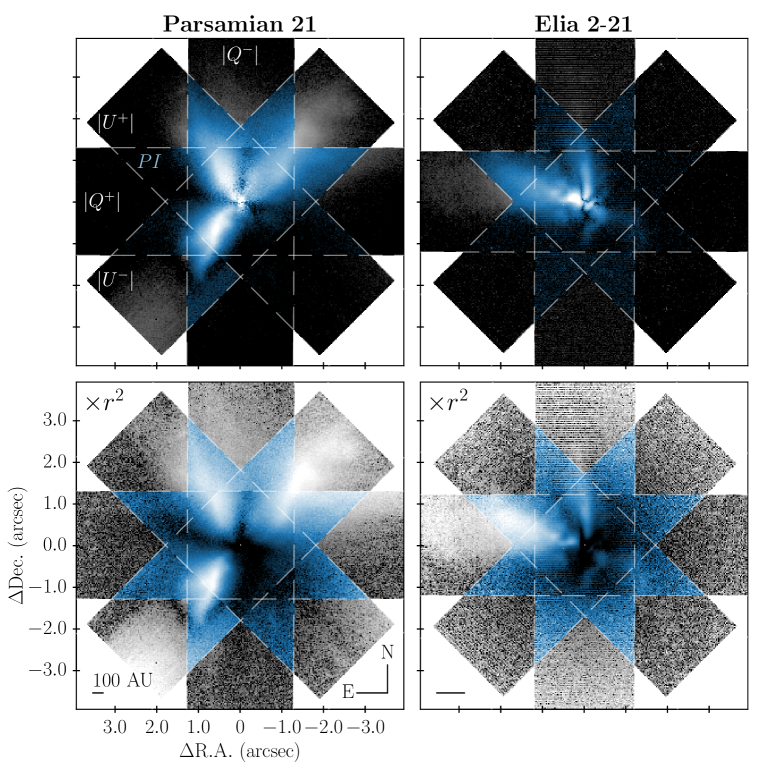
Figure 9: Polarised light for the embedded YSOs Parsamian 21 (left panels) and Elia 2-21 (right panels). The top panels show the polarised intensity, $PI,$ with a blue colour map, while the grey colours display the absolute values of the linear Stokes components $|Q^{\pm}|$ and $|U^{\pm}|$. In the bottom panels, these values are scaled by the squared separation from the centre. The dashed lines delineate the sections of the sky observed by one of the components. These sections overlap in the centre, resulting in an eight-pointed star, where the polarised intensity image can be computed as $Q$ and $U$ are both covered. The south-eastern region of the $U^{-}$ observation of Parsamian 21 is contaminated with signal from another dithering position, introduced during the sky-subtraction.

Observations that use PDI have revealed a large number of disks with different sizes, surface brightnesses, and morphologies in scattered light. Scattered light observations trace the upper layers of a circumstellar disk since the micron-sized dust grains found there are optically thick at optical and NIR wavelengths. Hence, circumstellar disks must be flared to intercept the stellar radiation at large distances (Chiang & Goldreich 1997; de Boer et al. 2016; Ginski et al. 2016). Transition disks with large dust-depleted inner cavities are frequently detected (e.g. Mayama et al. 2012; Canovas et al. 2013; Keppler et al. 2018; Maucó et al. 2020), and the observed circumstellar disks commonly show rings at varying radii (e.g. Quanz et al. 2013; Muro-Arena et al. 2018; Avenhaus et al. 2018). Additionally, spiral features are frequently detected in scattered light (see Fig. 9 of Benisty et al. 2023). The gas perturbations, coupled to the small grains that are traced in scattered light, are suggested to emerge from interactions with a companion or with the environment. Furthermore, the combination with sub-millimetre observations can reveal dust filtering at pressure maxima (e.g. Garufi et al. 2013; Maucó et al. 2020) and help identify fragmentation, possibly resulting from gravitational instability (Weber et al. 2023). In scattered light imaging, the misalignment of an (un-resolved) inner disk can cast a shadow onto the outer disk (Bohn et al. 2022). Depending on the magnitude of the misalignment, narrow shadow lanes (e.g. HD 100453; Benisty et al. 2017) or wide-angle obscurations can appear (e.g. HD 143006; Benisty et al. 2018). In the case of stellar multiplicity, the geometry of the circumstellar environment can be assessed further by interpreting which stellar component is responsible for the dust illumination (Weber et al. 2023; Zurlo et al. 2023). Depending on the size, composition, and porosity of the small dust grains, different scattering phase functions can be measured (Shen et al. 2009; Tazaki et al. 2016, 2019). By studying the dust properties in circumstellar disks, we can assess the efficiency of dust growth based on the size, composition, and porosity of the grains involved. PDI observations are not limited to Class II disks (Lada 1987): second-generation dust disks, or debris disks, are also observed with facilities such as VLT/SPHERE (e.g. HIP 79977; Engler et al. 2017, HR 4796A; Milli et al. 2019), Gemini South/GPI (e.g. HD 157587; Millar-Blanchaer et al. 2016), and Subaru/HiCIAO (e.g. HD 32297; Asensio-Torres et al. 2016).

For the most studied Class II disks (Lada 1987), the observed sub-structures are frequently explained by invoking the presence of planetary companions (e.g. ALMA Partnership et al. 2015; van der Marel et al. 2019; Long et al. 2019; Asensio-Torres et al. 2021). The existence of sub-structures suggests that planet formation is already underway and began when the YSOs were still embedded in their natal envelopes, during the Class 0 or I phases ($t<10^{6}\mathrm{\ yr}$; Garufi et al. 2022a). Furthermore, measurements of the dust masses of Class II disks appear incompatible with predicted planet formation efficiencies and the masses of exoplanetary systems (Manara et al. 2018; Mulders et al. 2021). The higher dust masses of Class 0 and I disks determined by Tychoniec et al. (2020) could indicate that giant planet formation commences before the protostellar envelope has dissipated (Cridland et al. 2022; Miotello et al. 2023). Alternatively, the accretion of material from the surrounding cloud can continually replenish the mass of the protoplanetary disk. The total mass budget available for planet formation therefore exceeds the disk mass at any given time (Manara et al. 2018; Garufi et al. 2022a). The two explanations put forward to solve the missing mass problem demonstrate the important role of embedded Class 0 and I objects in the formation of planets. However, the earliest YSOs are particularly difficult to observe at optical wavelengths due to their embedded nature. As a consequence, the optical wavefront sensors (WFSs) of most modern extreme adaptive optics (AO) systems do not allow for an adequate AO correction of deeply embedded YSOs. The NIR AO188 system, part of SCExAO on the Subaru telescope, is an exception as it provides AO for polarimetric imaging in the northern hemisphere. However, embedded protostars in the south were only observable to some older, ground-based instruments that were equipped with an infrared WFS. For completeness, the retired NICMOS instrument on the Hubble Space Telescope measured the polarised light of the earliest YSOs (e.g. Silber et al. 2000; Kóspál et al. 2008; Perrin et al. 2009), though JWST is not equipped with polarimetric capabilities.

In this work, we present a re-reduction of polarimetric archival data from NACO, the Nasmyth Adaptive Optics System (NAOS), which together with the COude Near-Infrared CAmera (CONICA) forms the NACO instrument at the VLT (Lenzen et al. 2003; Rousset et al. 2003). Initially installed at the Nasmyth B focus of UT4 in 2001, NACO was reinstalled at the Nasmyth A focus of UT1 from 2014 until its decommissioning in 2019. NACO operated at wavelengths between $1$ and $5\ \mu\mathrm{m,}$ and NAOS was equipped with a visible ($0.45$–$1.0\ \mu\mathrm{m}$) and infrared ($0.8$–$2.5\ \mu\mathrm{m}$) WFS, enabling observations of embedded YSOs despite their faint optical magnitudes. NACO was equipped with a Wollaston prism (and also wire grids; see Sect. 2.2.4) to perform polarimetric observations, and a half-wave plate (HWP) was installed in 2003. In Sect. 2 we describe how our PDI PiPelIne for NACO data (PIPPIN) reduces the NACO polarimetric data with the PDI technique. Section 3 outlines a broad inspection of the PIPPIN-reduced data, and we present a novel method for assessing the detection significance of a polarised signal. Section 4 compares the reduced data with those of the SPHERE instrument. The conclusions are summarised in Sect. 5, and the reduced data archive has been published online.

2 Reduction of NACO data

2.1 Selection of polarimetric observations

Since the polarimetric mode of NACO was not solely used to observe YSOs, we made a selection of observations of interest to this study. First, the European Southern Observatory (ESO) archive was searched for every polarimetric NACO observation classified as the SCIENCE data type. Using the object identifier and the astroquery Python package (Ginsburg et al. 2019), we searched the SIMBAD archive (Wenger et al. 2000) to select any object that was ever classified as one of the following categories: (candidate) Orion variable, (candidate) Herbig Ae/Be star, (candidate) T Tauri star, or a (candidate) YSO. However, a large number of observations have unclear object identifiers. In these instances, astroquery was utilised to locate the object closest to the target right ascension (RA) and declination (Dec.) coordinates. In total, we find 57 candidate Class 0 - III objects that potentially exhibit polarised light from circumstellar material. As these systems were observed in multiple filters, epochs, or with different instrument setups, we find a total of 243 datasets. Table LABEL:tab:systems lists the objects of interest and information on the observation setup for each dataset.

2.2 PDI PiPelIne for NACO data (PIPPIN)

A general pipeline to reduce NACO data is provided by ESO. However, this pipeline cannot reduce the polarimetric observations and thus previous works utilised custom, self-written pipelines (e.g. Apai et al. 2004; Quanz et al. 2011; Canovas et al. 2013). The different data reduction methods could lead to inconsistent scientific results. For instance, one of the rings of HD 97048 observed by Ginski et al. (2016) was not recovered from the same data in the earlier analysis of Quanz et al. (2012). Such discrepancies can be avoided by using a single, comprehensive pipeline. In this section, we describe the operation of our PIPPIN pipeline, which applies the PDI technique to polarimetric NACO observations. With the exception of an instrumental Mueller matrix model, PIPPIN largely follows the polarimetric data reduction outlined in de Boer et al. (2020). For a more detailed characterisation of the instrumental polarisation of NACO, we refer to de Boer et al. (2014) and Millar-Blanchaer et al. (2020).

2.2.1 FLATs, bad-pixel masks, and DARKs

To correct for any variations of the detector’s gain, PIPPIN performs a FLAT-fielding of the SCIENCE images. In general, internal lamp FLATs were taken for each filter and detector (i.e. S13, S27, L27, S54, and L54) that were used during the night. The polarimetric mask, which prevents the ordinary and extra-ordinary beams from overlapping, is also inserted when measuring the FLAT fields. The FLATs are DARK-subtracted and subsequently normalised by being divided by the median counts. The bad-pixel masks are generated by assessing which pixels had a non-linear response in the FLAT fields. The linearity of the pixel response is determined by comparing the FLATs observed with the internal lamp switched on ($\mathrm{FLAT}_{\mathrm{on}}$) to FLATs made with the lamp turned off ($\mathrm{FLAT}_{\mathrm{off}}$). The factor by which the pixel-counts are expected to increase is computed by dividing the median of $\mathrm{FLAT}_{\mathrm{on}}$ by the median of $\mathrm{FLAT}_{\mathrm{off}}$. Pixels were flagged when their response deviated by more than $2\sigma$ from the expected increase. Similar to the FLAT fields, the bad-pixel masks are computed for each filter and detector used throughout the night.

2.2.2 Pre-processing

The PIPPIN pipeline can be described in two parts: the pre-processing and the application of PDI. The pre-processing commences by reading parameters from a configuration file that allows users to customise the data reduction. The configuration file must be located in the same directory as the SCIENCE observations; otherwise, the pipeline creates a default file. Table 2 outlines the parameter keywords in the configuration file along with the recognised values, descriptions, and default values. After reading the configuration parameters, PIPPIN groups observations by the utilised detector, window-size, observing ID (if requested), filter, exposure time, HWP usage, and whether the Wollaston prism or wire grids were used. Each observation is DARK-subtracted and FLAT-normalised by division. The pixels flagged in the bad-pixel mask are replaced by the median counts of the surrounding square of $5\times 5$ pixels.

To retrieve the approximate positions of the ordinary and extra-ordinary beams, PIPPIN applies a minimum-filter with a specific kernel-shape to the images. The filter consists of two squares of $3\times 3$ pixels that are offset by the approximate separation of the beams, which in turn depends on the pixel scale of the utilised detector. The maximum in the filtered image yields the approximate location of the ordinary and extra-ordinary beams. This method avoids any persisting bad pixels or image artefacts such as the polarimetric mask. Subsequently, the initial guesses are used to retrieve more accurate PSF locations via a user-specified fitting method. For each beam, PIPPIN can employ a single 2D Moffat function or subtract two Moffat functions from each other to reproduce the flat top of a saturated PSF. Alternatively, the pipeline can use a maximum-counts method for the asymmetric PSFs that are encountered in the case of deeply embedded stars.

The sky-subtraction is performed by subtracting two dithering positions or by subtracting the median per row of pixels. To avoid contamination from the target, a region around the fitted beam centres is excluded in the median sky-subtraction method. This region is defined with the sky_subtraction_min_offset parameter in the configuration file. Moreover, this parameter ensures that the two dithering positions are sufficiently offset to perform a sky-subtraction. In addition, horizontal gradients are removed by a linear fit that excludes the region around the beams. The linear fit is applied to the average of five rows of pixels and a 2D Gaussian filter with $\sigma=5\ \mathrm{pixels}$ is applied to smooth out the resulting background approximation. Some observations show a distinct horizontal pattern, which can be removed by fitting each row of pixels individually and without applying a Gaussian filter. Next, the ordinary and extra-ordinary beams are cut out of the images by a user-specified crop-size. The maximum counts of the beams are evaluated with an iterative sigma-clipping to determine which observations suffered from a poor AO correction. Figure 1 shows an example of the open AO-loop analysis for observations of HD 135344B in the Ks band. The left panel shows the maximum counts of the ordinary and extra-ordinary beams for each observation in red and blue, respectively. The horizontal dashed lines show the $3\sigma$-bounds used in the sigma-clip. The right panels show examples of the ordinary beams of two observations. In this work, the images presented with a blue colour map show PIPPIN-reduced data products. The upper-right panel of Fig. 1 shows an effective AO correction and the lower-right panel shows an example of an open AO loop. In the bottom panel, we notice that the point source is blurred, likely as a result of a tilting wavefront during the integration. The resulting maximum count of the (extra-)ordinary beam is measured lower than the $3\sigma$-bound and this observation was removed. In this example, observations 3, 42, and 45 were ignored during the PDI application.

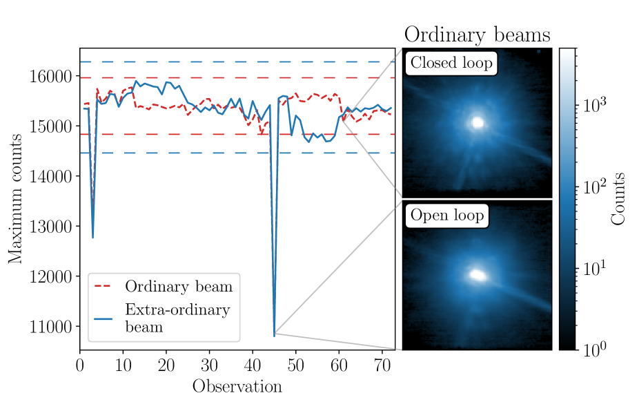
Figure 1: Open AO-loop assessment of HD 135344B Ks-band observations. Left panel: Maximum counts of the ordinary (red) and extra-ordinary (blue) beams. The horizontal dashed blue and red lines are the $3\sigma$ bounds for the respective beam, indicating which observations have adequate AO corrections. The upper-right panel shows an example of an effective AO correction for the ordinary beam, and the lower-right panel shows the blurred result of an open AO loop.

2.2.3 Polarimetric differential imaging

Polarised light can be described with the Stokes formalism and the Stokes vector:

(1)

(2)

(3)

(4)

,

where $I$ is the total intensity, $Q$ and $U$ are intensities of the linear polarisation components and $V$ describes the circular polarisation. As NACO was not primarily designed for polarimetry, the observations suffer from instrumental polarisation ($IP$) and crosstalk effects. Reflections within the instrument can introduce polarised signal whose magnitude depends on the instrument configuration, altitude of the target object, etc. Furthermore, crosstalk between the linear and circular polarisation components reduces the polarimetric efficiency (Witzel et al. 2011). Hence, PIPPIN employs a multi-stage correction for these effects. A first-order correction for different transmission efficiencies is to impose that the stellar flux in the ordinary ($I_{\mathrm{ord}}$) and extra-ordinary ($I_{\mathrm{ext}}$) beams are the same, as described in Appendix C of Avenhaus et al. (2014a). Since the PSF core is often saturated in NACO observations, PIPPIN draws multiple, user-specified annuli and computes the total fluxes within them. For each annulus $i$, the ratio between the fluxes,

$$X_{\mathrm{ord/ext},i}=\frac{\sum_{\mathrm{pixels}}I_{\mathrm{ord},i}}{\sum_{\mathrm{pixels}}I_{\mathrm{ext},i}},$$ (5)

is used to scale the ordinary and extra-ordinary images as $I_{\mathrm{ord}}/\sqrt{X_{\mathrm{ord/ext},i}}$ and $I_{\mathrm{ext}}\sqrt{X_{\mathrm{ord/ext},i}}$, respectively. This method implicitly assumes that the total flux in annulus $i$ is unpolarised, thereby ignoring any polarisation induced by the interstellar medium or any intrinsic polarisation originating from an unresolved inner disk, for example. We note that this correction could overcompensate for a true disk signal if the disk is not axisymmetric and if its scattered light comprises a considerable fraction of the stellar signal.

If the HWP has a rotation angle of $\theta=0^{\circ}$, the ordinary beam ($I_{\mathrm{ord}}$) measures light polarised in the $+Q$ direction and the extra-ordinary beam ($I_{\mathrm{ext}}$) measures the perpendicularly polarised light in the $-Q$ direction, both in the HWP reference frame. The $I_{Q}$ and $Q$ components are found by addition and subtraction of the equalised beam intensities:

$$I_{Q} =I_{\mathrm{ord}}+I_{\mathrm{ext}}\big{|}_{\theta=0^{\circ}},$$ (6)

$$Q =I_{\mathrm{ord}}-I_{\mathrm{ext}}\big{|}_{\theta=0^{\circ}}.$$ (7)

Measurements of the $U$ component are made by rotating the incoming beam by $45^{\circ}$, which means that the HWP is rotated by $\theta=22.5^{\circ}$. The $I_{U}$ and $U$ components are calculated with

$$I_{U} =I_{\mathrm{ord}}+I_{\mathrm{ext}}\big{|}_{\theta=22.5^{\circ}},$$ (8)

$$U =I_{\mathrm{ord}}-I_{\mathrm{ext}}\big{|}_{\theta=22.5^{\circ}}.$$ (9)

The top panels of Fig. 2 show the resulting median Stokes $Q$ and $U$ images for HD 135344B. The position angle (PA) is $-35^{\circ}$, so that the sky is rotated anti-clockwise to the axes of the detector as is indicated by the compasses in the figure. In the $Q$ image, the positive signal aligns with the Y-axis and the negative signal aligns with the X-axis. The $U$ image displays a similar butterfly pattern, but rotated by $45^{\circ}$ since it measures different components of the disk.

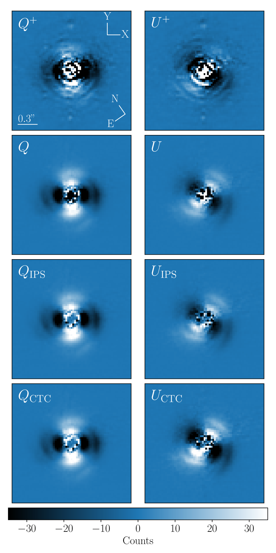
Figure 2: Median Stokes $Q$ and $U$ images with different levels of $IP$ corrections for HD 135344B Ks-band observations. From top to bottom: $Q^{+}$ and $U^{+}$ components after equalising the ordinary and extra-ordinary fluxes, $Q$ and $U$ resulting from the double-difference method, $Q_{\mathrm{IPS}}$ and $U_{\mathrm{IPS}}$ after subtracting the median $IP$ within an annulus, and the crosstalk-corrected $Q_{\mathrm{CTC}}$ and $U_{\mathrm{CTC}}$ components where the reduced Stokes $U$ efficiency is accounted for. The characteristic butterfly pattern is visible in each panel, and the compasses show the orientation of the detector and the sky.

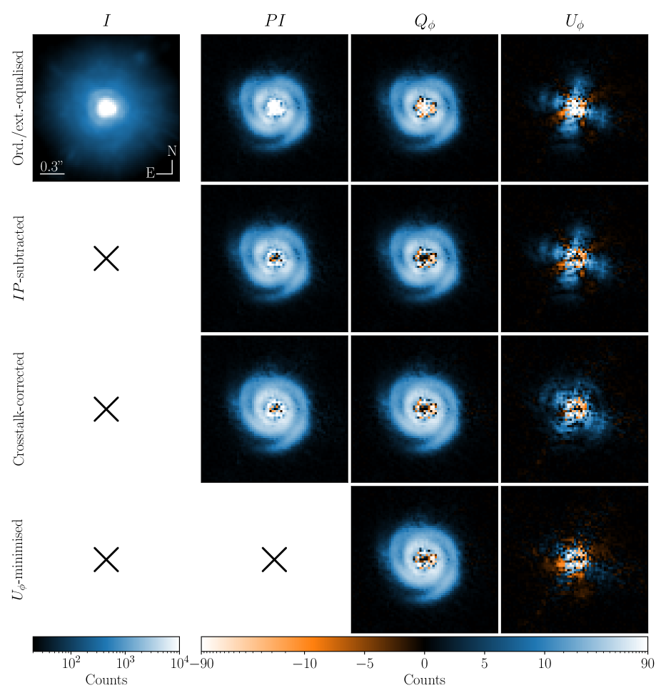
Figure 3: Final PIPPIN data products with different levels of $IP$ correction. From left to right: Median total intensity ($I)$, polarised intensity $(PI$), and the azimuthal Stokes components $Q_{\phi}$ and $U_{\phi}$ of HD 135344B observed in the Ks band. From top to bottom: Equalised ordinary and extra-ordinary beams, $IP$-subtracted, crosstalk-corrected, and $U_{\phi}$-minimised results. The total intensity is shown with a logarithmic scale from $20$ to $10^{4}$ counts, whereas the other panels use a linear scale from $-5$ to $+5$ counts and a logarithmic scale up to $\pm 90$. The negative signal is depicted in orange, and in each image north points up and east to the left.

Instrumental polarisation introduced downstream of the HWP can be removed by recording the $-Q$ and $-U$ parameters at $\theta=45^{\circ}$ and $67.5^{\circ}$, respectively. The instrumental $Q_{IP}$ and $U_{IP}$ components are unaffected by this rotation of the HWP and contribute in the same manner as before:

$$Q^{+} =Q+Q_{\mathrm{IP}} =I_{\mathrm{ord}}-I_{\mathrm{ext}}\big{|}_{\theta=0^{\circ}},$$ (10)

$$Q^{-} =-Q+Q_{\mathrm{IP}} =I_{\mathrm{ord}}-I_{\mathrm{ext}}\big{|}_{\theta=45^{\circ}},$$ (11)

$$U^{+} =U+U_{\mathrm{IP}} =I_{\mathrm{ord}}-I_{\mathrm{ext}}\big{|}_{\theta=22.5^{\circ}},$$ (12)

$$U^{-} =-U+U_{\mathrm{IP}} =I_{\mathrm{ord}}-I_{\mathrm{ext}}\big{|}_{\theta=67.5^{\circ}}.$$ (13)

Using the double-difference method (Hinkley et al. 2009; Bagnulo et al. 2009), we can subtract the $IP$ components:

$$Q =\frac{1}{2}(Q^{+}-Q^{-}),$$ (14)

$$U =\frac{1}{2}(U^{+}-U^{-}).$$ (15)

Similarly, the $IP$-corrected intensities are found with the double-sum:

$$I_{Q} =\frac{1}{2}(I_{Q^{+}}+I_{Q^{-}}),$$ (16)

$$I_{U} =\frac{1}{2}(I_{U^{+}}+I_{U^{-}}).$$ (17)

The total intensity is calculated as

$$I=\frac{1}{2}(I_{Q}+I_{U}).$$ (18)

The second row of Fig. 2 shows the median $Q$ and $U$ images resulting from the double-difference method. Due to the $IP$ removal, the butterfly patterns show more distinct features than the $Q^{+}$ and $U^{+}$ images and the recorded noise outside of the disk is reduced.

An additional correction is made for the $IP$ introduced upstream of the HWP, following the method outlined in Canovas et al. (2011) and de Boer et al. (2020). The correction is performed for each HWP cycle to mitigate temporal differences in the $IP$ as a result of changing angles of reflection. As before, it is assumed that the stellar light is unpolarised and polarised signal near the star is ascribed to instrumental polarisation (Quanz et al. 2011). The median $Q/I$ signal is computed over the same annulus $i$ from Eq. 5 to obtain a scalar $c_{Q}$. To obtain $c_{U}$, we calculate the median $U/I$ signal over the same annulus. Per annulus, the $IP$-subtracted linear Stokes components are found by subtracting the product of these scalars and the respective $I_{Q}$ or $I_{U}$ image:

$$Q_{\mathrm{IPS}} =Q-I_{Q}\cdot c_{Q},$$ (19)

$$U_{\mathrm{IPS}} =U-I_{U}\cdot c_{U}.$$ (20)

By using multiple user-specified annuli, the pipeline retrieves various $IP$-subtracted results. The third row of panels in Fig. 2 displays the median $Q_{\mathrm{IPS}}$ and $U_{\mathrm{IPS}}$ images where the annulus was drawn between a radius of 3 and 6 pixels. As expected from the correction, the $Q_{\mathrm{IPS}}$ measurement shows a decreased signal near the star compared to the $Q$ image.

In Fig. 2, the $U_{\mathrm{IPS}}$ signal is lower than $Q_{\mathrm{IPS}}$ as a result of crosstalk between the linear and circular Stokes components (Witzel et al. 2011). If a disk is unmistakably detected and approximately axisymmetric, this reduced efficiency of the Stokes $U$ component relative to $Q$ can be estimated following the method outlined by Avenhaus et al. (2014a). In an annulus with disk signal, the number of pixels where $|Q_{\mathrm{IPS}}|>|U_{\mathrm{IPS}}|$ is expected to be equal to the number of pixels where $|U_{\mathrm{IPS}}|>|Q_{\mathrm{IPS}}|$. We can multiply the $U_{\mathrm{IPS}}$ image by a factor of $1/e_{U}$ so that the above assumption holds. The crosstalk-corrected components are then

$$Q_{\mathrm{CTC}} =Q_{\mathrm{IPS}},$$ (21)

$$U_{\mathrm{CTC}} =\frac{1}{e_{U}}\cdot U_{\mathrm{IPS}},$$ (22)

where we assume an efficiency of $100\%$ for Stokes $Q$. By modelling the NACO $IP$ with standard star observations, Millar-Blanchaer et al. (2020) conclude that the Stokes $Q$ has an efficiency of $\sim$ $90\%$. Since such a correction is not performed with PIPPIN, any quantitative polarimetry measurements on the reduced data products could be off by $\sim$ $10\%$. The efficiency-correction should not be performed in instances with ambiguous signal and thus PIPPIN only makes the crosstalk-correction if requested.

Incomplete HWP cycles, with only measurements of $Q^{\pm}$ (or $U^{\pm}$), are removed. If only the Stokes $Q^{+}$ and $U^{+}$ (or only $Q^{-}$ and $U^{-}$) were recorded, PIPPIN will still be able to produce the final data products, but the double-difference method cannot be applied. At this point, the pipeline computes the median $Q$, $U$, $I_{Q}$, $I_{U}$, and $I$ over all observations. The final polarisation images ($PI$, $Q_{\phi}$, and $U_{\phi}$) are described below in terms of $Q$ and $U$, but we note that these data products are also calculated with $Q_{\mathrm{IPS}}$/$U_{\mathrm{IPS}}$ and $Q_{\mathrm{CTC}}$/$U_{\mathrm{CTC}}$, if possible. The total polarised intensity is calculated as

$$PI=\sqrt{Q^{2}+U^{2}}.$$ (23)

This method of squaring $Q$ and $U$ can lead to the increase in noise in regions where the $Q$ or $U$ signal originating from the disk is low. A cleaner image can be found with the azimuthal Stokes parameters outlined in Monnier et al. (2019) and de Boer et al. (2020), analogous to Schmid et al. (2006), but with a flipped sign:

$$Q_{\phi} =-Q\cos(2\phi)-U\sin(2\phi),$$ (24)

$$U_{\phi} =+Q\sin(2\phi)-U\cos(2\phi),$$ (25)

where $\phi$ is the azimuthal angle and is calculated for each pixel with

$$\phi =\arctan\left(\frac{\textit{y}-\textit{y}_{\mathrm{star}}}{\textit{x}_{\mathrm{star}}-\textit{x}}\right)+\phi_{0},$$ (26)

where ($\textit{x}_{\mathrm{star}}$, $\textit{y}_{\mathrm{star}}$) are the pixel-coordinates of the central star. If the disk has a low inclination and the scattered light emerges from single scattering events, the polarisation is oriented azimuthally with respect to the star. Consequently, the $Q_{\phi}$ image shows a positive signal as it measures polarisation angles of $\pm 90^{\circ}$. Simultaneously, the $U_{\phi}$ image is expected to show a negligible signal as it measures polarisation angles of $\pm 45^{\circ}$. However, a non-zero $U_{\phi}$ signal can occur if there is crosstalk between $Q$ and $U$, if the light is scattered multiple times (Canovas et al. 2015b), if the disk has a high inclination, and if an inadequate correction retains stellar or instrumental polarisation (Hunziker et al. 2021). If requested, PIPPIN can minimise the $U_{\phi}$ signal in the same annulus used for the crosstalk-correction by fitting for the azimuth angle offset $\phi_{0}$, similar to Avenhaus et al. (2014a). Otherwise, the offset angle $\phi_{0}$ is set to $0^{\circ}$.

The median total intensity $I$, polarised intensity $PI$, and azimuthal Stokes parameters $Q_{\phi}$ and $U_{\phi}$ with different levels of $IP$ correction are shown in Fig. 3 for HD 135344B. Once PIPPIN has computed the final data products, these images are de-rotated using scipy.ndimage.rotate. Therefore, contrary to Fig. 2, the panels of Fig. 3 have north pointing up and east to the left. It is apparent from the total and polarised intensity images that the PDI technique applies an extremely effective suppression of the stellar signal, thus revealing the circumstellar disk and its spiral arms. In this example, we observe the $U_{\phi}$ signal diminish as the $IP$ corrections are performed. Since HD 135344B is observed at a low inclination and axisymmetric to a first order, we employed crosstalk-correction and $U_{\phi}$ minimisation to produce the final Stokes images. For these Ks-band observations, we find a reduced efficiency of $e_{U}=0.65$, in agreement with Garufi et al. (2013) who find an efficiency of $0.61$ (Avenhaus et al. 2014a). Similarly, the more extensive $IP$ model presented by Millar-Blanchaer et al. (2020) results in an efficiency of $e_{U}=0.7\pm 0.02$ for Elia 2-25. Furthermore, we find an offset angle of $\phi_{0}=5.3^{\circ}$, while $3.7^{\circ}$ is derived in the previous analysis of these data (Garufi et al. 2013; Avenhaus et al. 2014a).

2.2.4 Non-HWP and wire-grid observations

Prior to August 8, 2003, NACO was not equipped with a HWP. Rather than rotating the HWP to modulate the direction of polarisation, observers would alter the PA by rotating the instrument on its rotator ring. PIPPIN automatically diagnoses whether the de-rotator flange of the telescope support structure was used (Lenzen et al. 2003). For these data, the HWP angles $\theta=0$, $22.5$, $45$, and $67.5^{\circ}$ in Eqs. 10, 11, 12, and 13 are replaced by the PAs of the instrument: $\theta_{PA}=0$, $45$, $90$, and $135^{\circ}$. The $Q^{\pm}$, $U^{\pm}$, $I_{Q^{\pm}}$, and $I_{U^{\pm}}$ images are also de-rotated to align the circumstellar structures before combining them with Eqs. 14, 15, 16, and 17. For the rotator observations, the $IP$ subtraction of Eqs. 19 and 20 is also performed.

In the early stages of its operation, NACO was equipped with wire grids to carry out polarimetric observations, rather than the Wollaston prism. In our cross-validation of the ESO archive, we found four potentially young sources that were observed in this manner: V1647 Ori, NX Pup, Mon R2 IRS 3, and R Mon. PIPPIN adopts the Pol_00, Pol_45, Pol_90, and Pol_135 wire grids as measurements of the Stokes $Q^{+}$, $U^{-}$, $Q^{-}$, and $U^{+}$ components, respectively. The linear Stokes components are propagated in the presence of the HWP. The only beam that is present in the images is fit with a single Moffat function. Since the wire-grid observations are not limited by the height of the polarimetric mask, their final data products have a much larger field of view than those obtained with the Wollaston prism.

2.2.5 Supplemental data products

Since the disk is illuminated by the star, the scattered light brightness decreases by the inverse of the squared distance to the host star. To better visualise structures at larger separations from the star, PIPPIN also produces images that are multiplied by the squared, de-projected radius. The disk PA, $PA_{\mathrm{disk}}$, is used to calculate the offsets along the major axis, $\Delta\textit{x}_{\mathrm{disk}}$, and minor axis, $\Delta\textit{y}_{\mathrm{disk}}$, with

$$\Delta\textit{x}_{\mathrm{disk}} =\Delta(\mathrm{R.A.})\cdot\sin PA_{\mathrm{disk}}+\Delta(\mathrm{Dec.})\cdot\cos PA_{\mathrm{disk}},$$ (27)

$$\Delta\textit{y}_{\mathrm{disk}} =\Delta(\mathrm{Dec.})\cdot\sin PA_{\mathrm{disk}}-\Delta(\mathrm{R.A.})\cdot\cos PA_{\mathrm{disk}},$$ (28)

where $\Delta(\mathrm{R.A.})$ and $\Delta(\mathrm{Dec.})$ are the right ascension and declination offsets with respect to the star. Subsequently, the de-projected radius $r$ is computed with

$$r =\sqrt{\Delta\textit{x}_{\mathrm{disk}}^{2}+\left(\frac{\Delta\textit{y}_{\mathrm{disk}}}{\cos i_{\mathrm{disk}}}\right)^{2}},$$ (29)

where $i_{\mathrm{disk}}$ is the disk inclination. As is shown in Table 2, the disk PA, $PA_{\mathrm{disk}}$ and inclination $i_{\mathrm{disk}}$ are specified in the configuration file for PIPPIN and are set to $0^{\circ}$ by default. In cases where the disk inclination and PAs are unknown, the default values ensure that the images are scaled by the projected separation from the host star.

The height of the final data products is limited to $\sim$ $3.0\ \mathrm{arcsec}$ (using the S27 detector) due to the polarimetric mask. Observations where the PA was rotated, rather than the HWP, cover a larger area of the sky. Since the sky rotates while the polarimetric mask remains stationary, the effective field of view is increased. Figure 9 depicts this increased sky coverage. An eight-pointed star emerges where at least one $Q$ and one $U$ component are covered and thus the polarised intensity can be computed within this shape. An inner octagon appears where every positive and negative Stokes component is observed. We note that the signal-to-noise decreases for areas outside of this octagon, due to the reduced number of observations. PIPPIN outputs the extended eight-pointed star images in addition to the data products resulting from the double-difference method, which are restricted to the inner octagon that has a complete coverage.

3 Inspection of NACO data

3.1 Identification of detections

The PIPPIN pipeline described above was used to reduce all observations listed in Table LABEL:tab:systems. The table lists multi-epoch, multi-wavelength observations as well as different exposure times and whether the wire grids were used or the Wollaston prism, with the HWP or PA. For each set of observations, we indicate the (non-)detection of circumstellar material in the final data products. The detection significance of polarised signal was assessed via a template-matching method, akin to cross-correlation, applied to the Stokes Q and U images. In the case of a detection, we expect that the signal is present in multiple, adjacent pixels and forms a specific butterfly pattern. Synthetic $Q_{\mathrm{synth}}$ and $U_{\mathrm{synth}}$ templates of the expected butterfly patterns were constructed with

$$Q_{\mathrm{synth}} =-\cos\big{(}2(\phi-PA)\big{)},$$ (30)

$$U_{\mathrm{synth}} =-\sin\big{(}2(\phi-PA)\big{)},$$ (31)

where $\phi$ is the azimuthal angle calculated with Eq. 26 and $PA$ is the position angle of the observation, which is subtracted since PIPPIN de-rotates the final data products, including the $Q_{\mathrm{IPS}}$ and $U_{\mathrm{IPS}}$ images. Subsequently, the $Q_{\mathrm{synth}}$ and $U_{\mathrm{synth}}$ templates were divided into multiple annuli with increasing radius and width of $2\ \mathrm{pixels}$, roughly corresponding to one resolution element in the H ($42\ \mathrm{mas}$) and Ks band ($56\ \mathrm{mas}$) at a pixel scale of $27\ \mathrm{mas\ pixel^{-1}}$. Figure 4 shows an example of the $Q_{\mathrm{synth}}$ and $U_{\mathrm{synth}}$ templates and a single annulus for a PA of $-35^{\circ}$, corresponding to the observations of HD 135344B. The values in the templates range from $-1$ to $+1$ and pixels outside of the annulus are set to $0$, thus ensuring that they do not contribute when calculating the cross-correlation coefficient. In annulus $i$, a cross-correlation coefficient is calculated for the $Q$ and $U$ signals:

$$CC_{Q,i} =\sum_{\mathrm{pixels}}Q_{\mathrm{IPS},i}\cdot Q_{\mathrm{synth},i},$$ (32)

$$CC_{U,i} =\sum_{\mathrm{pixels}}U_{\mathrm{IPS},i}\cdot U_{\mathrm{synth},i},$$ (33)

where the sum is performed over every pixel within annulus $i$. In this manner, a positive pixel increases the coefficient if the respective quadrant expects a positive signal. A negative signal in the negative quadrants of the template also contributes, whereas a discrepant signal reduces the cross-correlation coefficient. A cross-correlation function (CCF) is constructed by computing a coefficient for each annulus. For the narrowband NB_1.64 observations of HD 135344B, the rightmost panel of Fig. 5 displays the CCFs for the $Q_{\mathrm{IPS}}$ and $U_{\mathrm{IPS}}$ components in blue and red, respectively. The CCF was converted into a signal-to-noise ($\mathrm{S/N}$) function by subtracting the mean coefficient between $35$ and $50$ pixels, and subsequently dividing by the standard deviation of coefficients within that same range, indicated by the grey shaded region in the right panel. The annulus-wise CCFs peak at a radius of 8 pixels with signal-to-noises of $\mathrm{S/N}\sim$ $13$ and $\sim$ $15$, respectively for $Q_{\mathrm{IPS}}$ and $U_{\mathrm{IPS}}$. These maxima surpass our $5\sigma$ detection threshold, thereby identifying this observation as a detection. Although the template-matching method generally worked well, it failed to flag two observations of HR 4796 as detections, despite the polarised signal evident from a visual inspection. These non-detections can be ascribed to the high inclination and narrow features of HR 4796, while the outlined template-matching analysis works optimally for face-on disks.

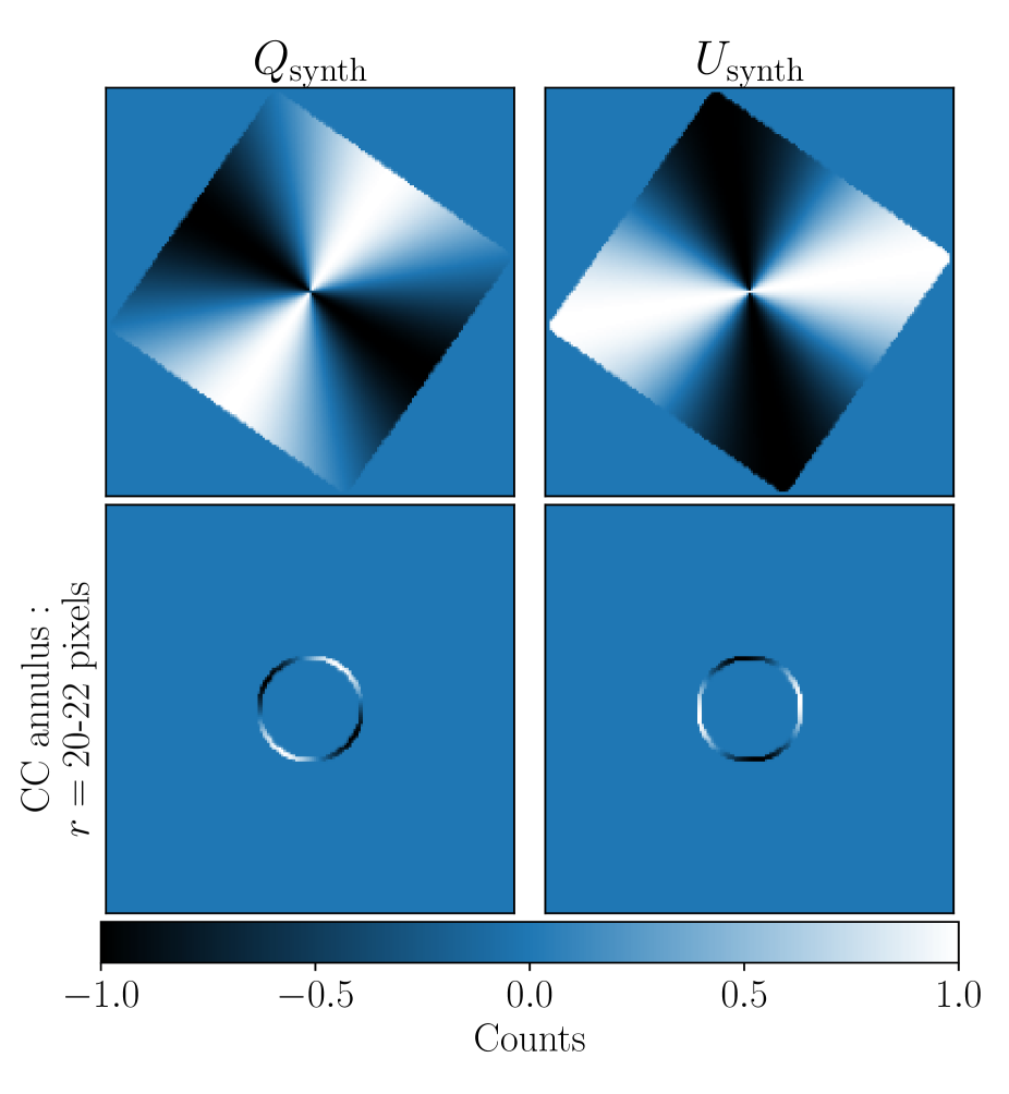
Figure 4: Templates for observations of HD 135344B with a PA of $-35^{\circ}$. Top panels: Complete $Q_{\mathrm{synth}}$ and $U_{\mathrm{synth}}$ templates. Values range from $-1$ to $+1,$ and pixels outside of the image are set to $0$. Bottom panels: Example annuli used in computing the cross-correlation coefficients.

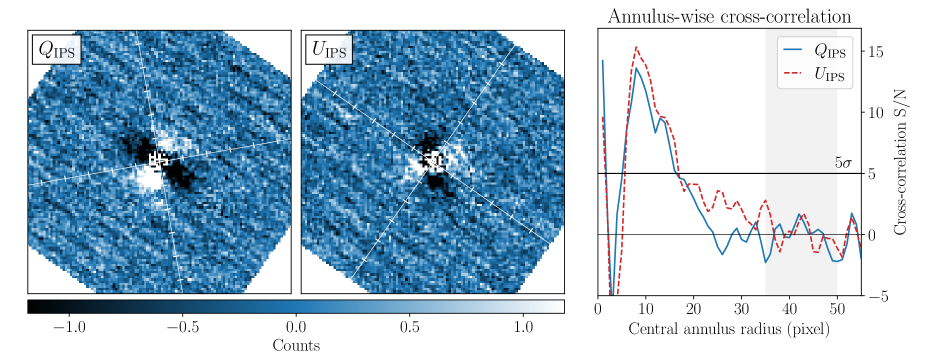
Figure 5: Detection analysis of HD 135344B observed in the narrowband NB_1.64. Left panels: $Q_{\mathrm{IPS}}$ and $U_{\mathrm{IPS}}$ images divided by the white lines into the four quadrants of the expected butterfly pattern. Right panel: Annulus-wise CCFs, with the $\mathrm{S/N}$ shown against the annulus radius in pixels. The results for the $Q_{\mathrm{IPS}}$ and $U_{\mathrm{IPS}}$ images are plotted in blue and red, respectively. The shaded region specifies the coefficients used in normalising and converting the CCF into a $\mathrm{S/N}$ function. The $5\sigma$ detection limit is indicated with a horizontal line.

In this reduction of the NACO data, many of the non-detections are likely the result of small or faint disks, or the absence of polarised light. Notably, IM Lup, GQ Lup, and EX Lup do not show polarised light in the NACO data, despite their prominent detections with SPHERE/IRDIS (Avenhaus et al. 2018; van Holstein et al. 2021; Rigliaco et al. 2020). The data of IM Lup and GQ Lup were not previously published, whereas Kóspál et al. (2011) also report a non-detection of polarised light in the EX Lup observations.

3.2 Analysis of detected polarised light

As demonstrated in Table LABEL:tab:systems, in 22 out of the 57 observed systems, we find at least one set of observations with polarised signal originating from circumstellar material. Figure 6 presents a gallery of these detections and highlights a diverse collection of morphologies. As mentioned in Sect. 2, HD 135344B shows distinct spiral arms in its circumstellar disk while HD 142527 has spiral features in its eastern and western lobes. Furthermore, we detect rings in a large number of disks, including HD 169142, HD 163296, HD 97048, HR 4796, TW Hya, HD 142527, and Sz 91. HR 4796 is the only debris disk in our sample and its $Q_{\phi}$ image shows a narrow ring. The disks around HD 163296, HD 97048, and HD 100546 are offset from the central star, suggesting that the scattering surface is above the disk midplane as confirmed by Monnier et al. (2017), Ginski et al. (2016), and Sissa et al. (2018). The highly extended disk of HD 142527 shows a large inner cavity that is possibly cleared out by an inner companion (Biller et al. 2012; Close et al. 2014; Lacour et al. 2016; Claudi et al. 2019), undetected in polarised light. Moreover, we find narrow shadow lanes imprinted on the disks of HD 142527 and SU Aur, similar to Avenhaus et al. (2017) and Ginski et al. (2021). In these cases, misaligned inner disks prevent the stellar light from reaching certain areas of the outer disk. CR Cha, MP Mus, AK Sco, and Elia 2-25 show negligible structure due to their small sizes, but a significant butterfly pattern was detected, leading to their inclusion in Fig. 6. As a possible consequence of their small sizes, the polarimetric NACO data of CR Cha and MP Mus were previously unpublished.

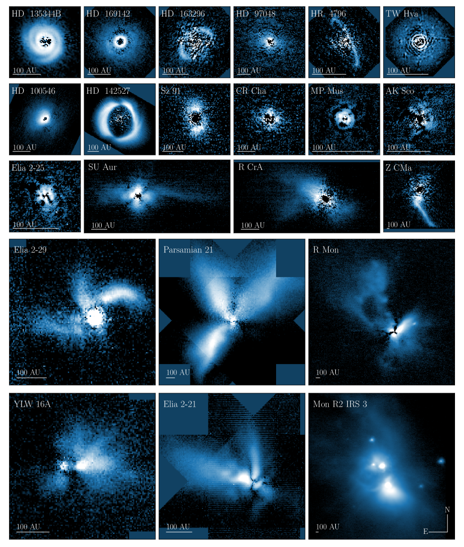
Figure 6: Gallery of young systems detected with NACO and reduced with PIPPIN. Each panel shows the polarised light on a logarithmic scale ranging between different values to highlight sub-structures. The highest degree of $IP$ correction is used where possible. Scale bars in the lower-left corners of each panel indicate $100\ \mathrm{AU}$ at each object’s distance. HD 169142, R CrA, and Parsamian 21 are shown in the H band, MP Mus is shown in the IB_2.06 filter, and the other panels use Ks-band observations. Mon R2 IRS 3 shows the median $I_{Q}$ image because the Stokes $U$ component was not observed. The images of YLW 16A and Elia 2-21 present the first polarised light detections in the NACO observations.

Figure 6 displays a number of objects with extended features that appear inconsistent with circumstellar disks. SU Aur shows tail-like features, where Ginski et al. (2021) discover an inflow of material onto the disk by combining polarimetric SPHERE observations with ALMA line observations. The features of R CrA resemble the non-polarimetric SPHERE observations presented by Mesa et al. (2019) with scattered light towards the north-east, south-east, and south-west of the primary star. Although a brightness asymmetry is observed towards the east in the NACO $Q_{\phi}$ image, the companion inferred by Mesa et al. (2019) is not detected. To our knowledge, the detection of polarised light in the NACO observations of R CrA went unpublished before this work. Recently, Dong et al. (2022) reported that the binary star Z CMa experienced a close encounter with a nearby star (masked in the NACO observation), thereby ejecting the streamer structure that we also observe in the $Q_{\phi}$ image. As YLW 16A, Elia 2-29, Elia 2-21, and Parsamian 21 were observed with the rotator flange, Fig. 6 presents the extended data products described in Sect. 2. The polarised light of Elia 2-29 reveals three arcs to the east, north and north-west of the central star. The northern and north-western arcs have curved shapes that are reminiscent of spiral-like features (Huélamo et al. 2007). YLW 16A shows asymmetric polarised signal to the west and north-west of the binary components (Plavchan et al. 2013) that are still visible as intensity maxima. Parsamian 21 and Elia 2-21 appear to show bipolar outflows along the NW-SE and NE-SW axes, respectively. Both nebulae are distinctly asymmetric with the northern and north-eastern segments showing the largest emission surfaces, respectively for Parsamian 21 and Elia 2-21. At large separations, along the PAs of the $Q^{\pm}$ and $U^{\pm}$ measurements, one of the linear Stokes components dominates over the other. Hence, the majority of the signal in $PI$ can be represented by the absolute values $|Q^{\pm}|$ or $|U^{\pm}|$, which is shown with a grey colour map in Fig. 9. The northern lobe of Parsamian 21 and the northern and eastern arms of Elia 2-21 are traced about $\sim$ $2\ \mathrm{arcsec}$ further. To our knowledge, this work is the first publication of the polarimetric NACO observations of Elia 2-21 and YLW 16A. The polarised light of the reflection nebula NGC 2261, illuminated by R Mon, demonstrates distinct emission from the extended north-eastern and south-western components. The Stokes U component of the infrared source Mon R2 IRS 3, part of the Monoceros R2 molecular cloud complex, was not observed. Hence, Fig. 6 presents the median $I_{Q}$, which also includes unpolarised (scattered) light. Despite this, filamentary structure is unambiguously detected. As discussed in Sect. 2.2.4, the two detections utilising polarimetric wire grids, R Mon and Mon R2 IRS 3, have much larger image sizes than the regular data products (i.e. compared to the upper rows of panels in Fig. 6).

3.3 Disk classification and brightness

Circumstellar polarised light is detected in nine out of the 14 Herbig stars in our sample. Grouping the Orion variables together with T Tauri stars, we detect polarised signal in eight out of 28 systems. For the YSOs, five of the 14 sources are flagged as detections with the template-matching analysis. The only high-proper motion star in our sample, HR 4796, also constitutes the only detection of a debris disk. However, our selection of young stars based on the SIMBAD object type could have missed some of the older Class III disks. Since NACO frequently observed disks known to be extended and thus potentially observable in scattered light, the gathered sample is certainly not unbiased. For that reason, a statistical analysis of the disk occurrence per object type is somewhat arbitrary.

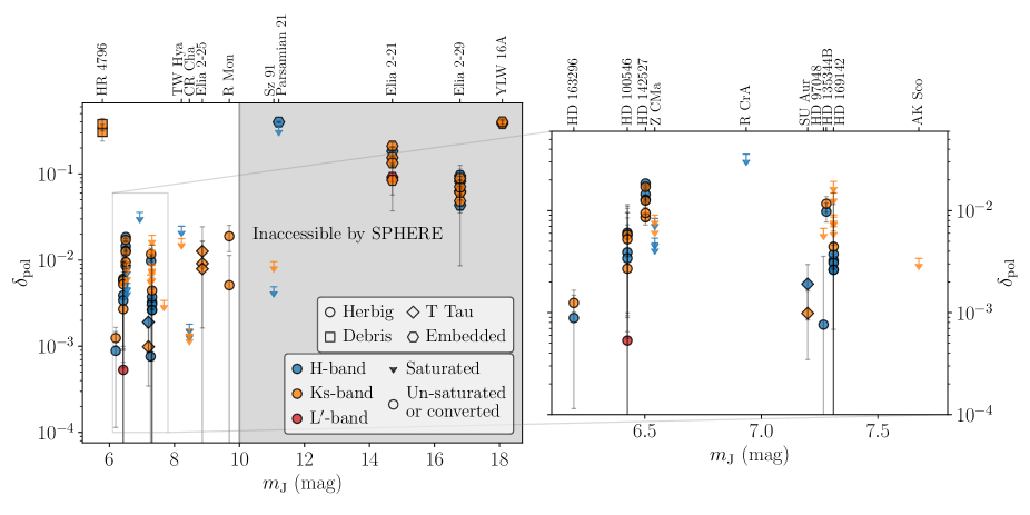
Figure 7: Polarised-to-stellar light contrast, $\delta_{\mathrm{pol}}$, plotted against the apparent J-band magnitude. The right panel shows a zoomed-in view of the bright $m_{\mathrm{J}}$. The object names are listed along the top axes. The marker colours and symbols specify the observing filter and object type, respectively. Upper limits are shown when the stellar PSF was determined to be saturated. The error bars show the $3\sigma$ uncertainties. The grey shaded region shows the approximate magnitudes ($m_{\mathrm{J}}\gtrsim 10$) inaccessible by the SPHERE AO system.

Here we examine the disk brightness of the sample of circumstellar disks detected by NACO. Since the disk inclination, disk extent, stellar brightness, and the distance to the source affect the total disk brightness, we made use of the polarised-to-stellar light contrast $\delta_{\mathrm{pol}}$ (Garufi et al. 2017, 2022b; Benisty et al. 2023). The polarised flux per unit area, $F_{\mathrm{pol}}$, was multiplied by the squared separation $4\pi r^{2}$ to account for the reduced stellar illumination. Subsequently, we normalised it by the stellar flux $F_{*}$ and averaged radially along the disk’s major axis. Thus, the polarised-to-stellar light contrast was computed as

$$\delta_{\mathrm{pol}} =\frac{1}{r_{\mathrm{out}}-r_{\mathrm{in}}}\cdot\int_{r_{\mathrm{in}}}^{r_{\mathrm{out}}}\frac{F_{\mathrm{pol}}(r)}{F_{*}}\cdot 4\pi r^{2}dr,$$ (34)

where $r_{\mathrm{in}}$ and $r_{\mathrm{out}}$ are the inner- and outermost radii, respectively. This measurement expresses the fraction of stellar photons that became polarised as a result of scattering by the resolved disk. The contrast $\delta_{\mathrm{pol}}$ is set by the geometry and composition of the circumstellar disk and is sometimes referred to as the geometrical albedo. Following the method outlined in Appendix B of Garufi et al. (2017), we performed a 2-pixel-wide cut (one resolution element) of the $Q_{\phi}$ image along the major axis of the disk. The photons measured along the major axis are scattered with angles close to $90^{\circ}$. This cut reduces the impact of the disk inclination on its brightness due to any asymmetry in the scattering phase function. The PA of the major axis varies for the sources observed by NACO, but was set to $0^{\circ}$ when this axis could not be estimated. These ambiguous sources (e.g. CR Cha) were roughly azimuthally symmetric and therefore did not significantly affect the derived contrast. The inner- and outermost radii ($r_{\mathrm{in}}$, $r_{\mathrm{out}}$) were determined by eye for each system detected in scattered light. The disk inclination and scale height were not taken into account when re-scaling the polarised flux by the projected separation. Similar to Garufi et al. (2017), we calculated the primary error of $\delta_{\mathrm{pol}}$ by deriving the standard deviation in a resolution element of the $Q_{\phi}$ image. Subsequently, this noise estimate for each pixel was propagated through Eq. 34 to find $\sigma_{\delta_{\mathrm{pol}}}$.

Fig. 7 displays the polarised-to-stellar light contrast $\delta_{\mathrm{pol}}$ against the apparent J-band magnitude $m_{\mathrm{J}}$, measured as part of the 2 Micron All Sky Survey (2MASS; Cutri et al. 2003). The source names are shown along the top axes. Blue, orange, and red markers indicate whether the observation was performed in the H, Ks, or L’ band. Diamonds (T Tau), circles (Herbig), and squares (debris) mark the object types. We note that HD 135344B is shown as a Herbig star (circle), in line with Garufi et al. (2014), but contrary to the SIMBAD object type in Table LABEL:tab:systems. Similarly, Parsamian 21 is depicted as an embedded YSO despite its Orion variable type reported in Table LABEL:tab:systems. The $\delta_{\mathrm{pol}}$ values of saturated PSFs are presented as upper limits in Fig. 7 (triangles; 99.75-th percentile) because the stellar flux $F_{*}$ is underestimated. In some instances, the source was also observed with narrowband filters where the stellar PSF was not saturated due to the smaller filter width. Hence, we could estimate the broadband flux $F_{*}^{\mathrm{BB}}$, using the narrowband flux $F_{*}^{\mathrm{NB}}$, if the two filters had overlapping wavelength ranges. We calculated the stellar flux as

$$F_{*}^{\mathrm{BB}} =F_{*}^{\mathrm{NB}}\cdot\frac{t_{\mathrm{exp}}^{\mathrm{BB}}}{t_{\mathrm{exp}}^{\mathrm{NB}}}\cdot\frac{\int T^{\mathrm{BB}}(\lambda)\ \mathrm{d}\lambda}{\int T^{\mathrm{NB}}(\lambda)\ \mathrm{d}\lambda},$$ (35)

where $t_{\mathrm{exp}}^{\mathrm{BB}}$ and $t_{\mathrm{exp}}^{\mathrm{NB}}$ are the exposure times of the broadband and narrowband observations, respectively. We integrated over the corresponding transmission curves $T(\lambda)$ to estimate how many photons should be detected for each photon in the narrowband filter. For the H band, we used the NB_1.64 and NB_1.75 narrowband filters. For the Ks band, NB_2.17, IB_2.18, NB_2.12, NB_2.15, and IB_2.21 were employed to compute the broadband flux and the NB_3.74 filter was used for saturated L’-band observations.

Since NACO was equipped with a NIR WFS, it could observe sources down to $\mathrm{K}\approx 14\ \mathrm{mag}$ (Rousset et al. 2003). For comparison, SPHERE’s optical WFS has a magnitude limit of $\mathrm{R}\approx 14\ \mathrm{mag}$ (Beuzit et al. 2019), GPI has a limit of $\mathrm{I}\approx 10\ \mathrm{mag}$ (Macintosh et al. 2014), and SCExAO/CHARIS on the Subaru telescope is limited by $\mathrm{R}\approx 13\ \mathrm{mag}$. For that reason, NACO could achieve a unique insight into embedded protostars, despite their faint optical magnitudes. The grey shaded region in Fig. 7 roughly indicates the sources that are inaccessible by the optical WFS installed on SPHERE. Since the estimated J-band magnitude limit of SPHERE depends on the spectral type of the observed source, the limit of $m_{\mathrm{J}}\sim$ $10\ \mathrm{mag}$ should be viewed as a crude assessment. From Fig. 7 we find that the four embedded protostars Parsamian 21, Elia 2-21, Elia 2-29, and YLW 16A, in addition to the low-mass star Sz 91, are likely not observable with modern PDI instruments.

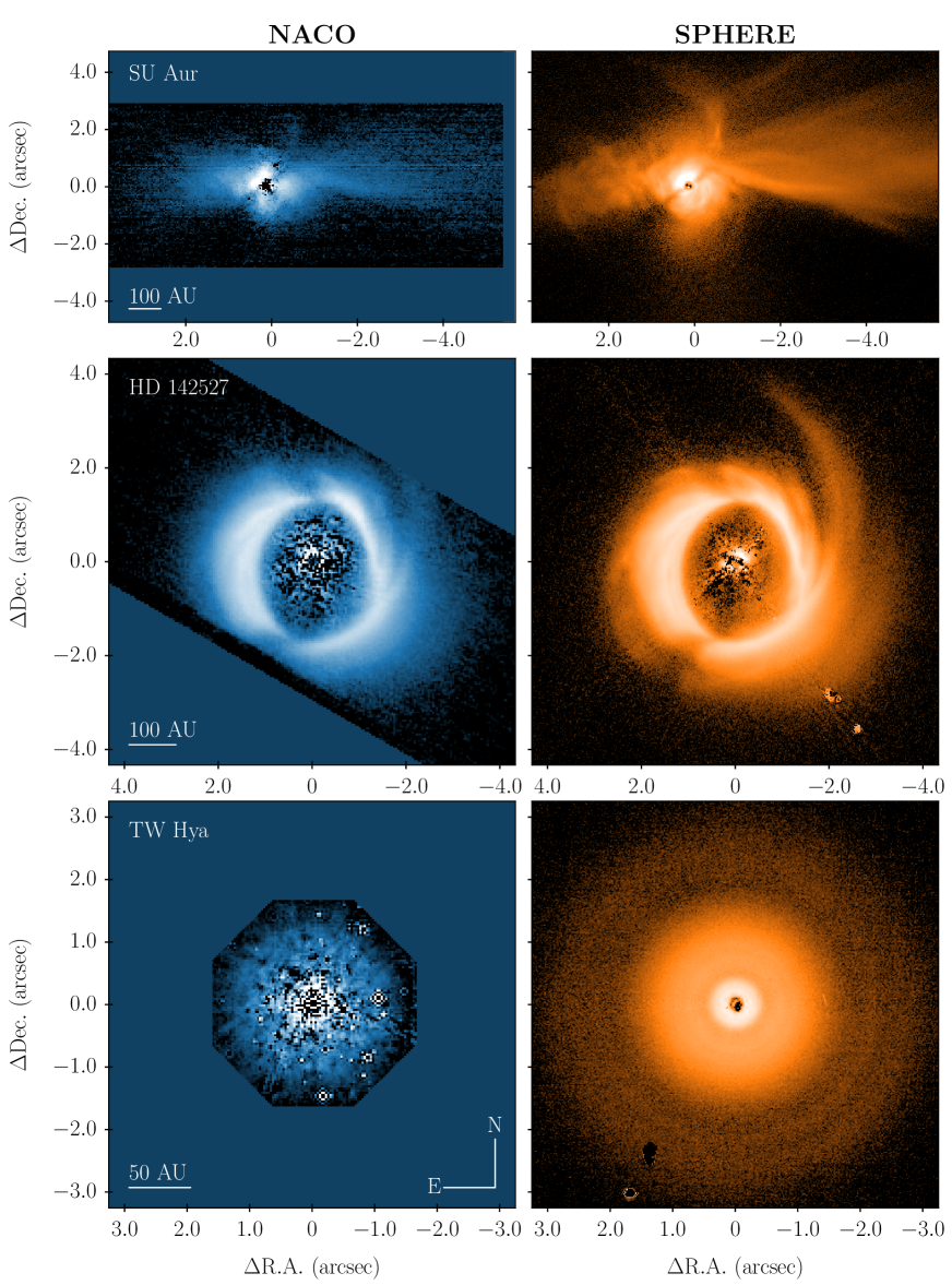
Figure 8: Comparison between PIPPIN-reduced NACO $Q_{\phi}$ observations (left panels) and the more recent SPHERE data (right panels). From top to bottom: SU Aur, HD 142527, and TW Hya observed in the H band with both instruments. The SPHERE observations were previously published by Ginski et al. (2021), Hunziker et al. (2021), and van Boekel et al. (2017) for SU Aur, HD 142527, and TW Hya, respectively.

The polarised-to-stellar light contrasts $\delta_{\mathrm{pol}}$ are listed in Table LABEL:tab:systems. We note that the $\delta_{\mathrm{pol}}$ values are possibly underestimated by $\sim$ $10\%$ (see Sect. 2.2.3) due to the absence of a correction for the reduced $Q$ efficiency resulting from crosstalk. For the sources with available mass estimates (also included in Table LABEL:tab:systems), we fail to detect a trend between $\delta_{\mathrm{pol}}$ and the stellar mass $M_{*}$. Since the disk’s dust mass is related to the stellar mass (e.g. Pascucci et al. 2016), the absence of a distinct trend reveals that the disk brightness in polarised light is not strongly correlated with the abundance of dust in the system. Instead, the scattered light brightness is affected by the amount of light that is intercepted. The geometry of the system primarily influences the polarised-to-stellar light contrast $\delta_{\mathrm{pol}}$, with the dust composition acting as a secondary effect. Similarly, Garufi et al. (2022b) find no correlation between the disk brightness in scattered light and dust mass estimated from the $1.3\ \mathrm{mm}$ flux. We also find no apparent distinction in disk brightnesses between the T Tauri stars and Herbig stars. Comparing the obtained $\delta_{\mathrm{pol}}$ results with those presented in Fig. 3 of Garufi et al. (2022b) and Table A.1 of Garufi et al. (2017), we find good agreement for HD 163296, HD 100546, HD 142527, HD 97048, HD 135344B, HD 169142, AK Sco, TW Hya, and CR Cha. For the extended systems SU Aur, R CrA, and Z CMa, we assessed the polarised-to-stellar light contrast ratio of a potential disk component at close separations, meaning that $r_{\mathrm{out}}$ was limited to $25$, $25,$ and $53$ pixels, respectively. We find $\delta_{\mathrm{pol}}\sim$ $1.5\cdot 10^{-3}$ for SU Aur, $\lesssim 3\cdot 10^{-2}$ for R CrA, and $\lesssim 6\cdot 10^{-3}$ for Z CMa. The brightest disk is found around HR 4796 with $\delta_{\mathrm{pol}}\sim$ $0.3-0.4$. This finding is somewhat surprising, given that it is a flat debris disk and therefore should not intercept much stellar light. However, the high brightness is also reported in previous works where it is argued that the scattering phase functions are consistent with large ($\sim$ $20\ \mathrm{\mu m}$) aggregate dust particles composed of small monomers (Milli et al. 2017, 2019). For Sz 91, the lowest-mass star ($M=0.58\pm 0.07M_{\odot}$; Maucó et al. 2020) where polarised light is detected, we determine upper limits of $\delta_{\mathrm{pol}}\lesssim 8\cdot 10^{-2}$ and $\lesssim 4\cdot 10^{-2}$ in the Ks and H band, respectively. The estimated contrasts of multi-wavelength observations do not show any clear discrepancies between H- and Ks-band observations, owing to relatively large uncertainties. Hence, it is difficult to draw any conclusions about the dust composition by evaluating the disk colour.

4 Discussion

The morphologies shown in Fig. 6 are almost identical to the polarised intensity images presented in previous publications of these data (see Table LABEL:tab:systems for references). The data reduction performed by PIPPIN therefore appears to reproduce the results obtained by the custom pipelines in other works.

To study the performance between different instruments, Fig. 8 presents a comparison between the NACO and modern SPHERE observations of SU Aur (programme ID: 1104.C-0415(E), PI: Ginski), HD 142527 (programme ID: 099.C-0601(A), PI: Avenhaus), and TW Hya (programme ID: 095.C-0273(D), PI: Beuzit). In this comparison, we find the results of the different instrument characteristics. For instance, the NACO observations of TW Hya were made under better seeing conditions ($\sim$ $0.5\ \mathrm{arcsec}$) than those made by SPHERE ($\sim$ $0.7\ \mathrm{arcsec}$), but we find that the NACO polarised signal displays residual speckles over the circumstellar disk. The SPHERE $Q_{\phi}$ image does not show similar artefacts, likely due to the superior AO instrument. As part of the NACO instrument, NAOS had fewer actuators ($185$ active actuators for NAOS against $1377$ for SAXO; Blanco et al. 2022) shaping the deformable mirror and its optical WFS operated at a lower frequency ($1200\ \mathrm{Hz}$ versus $444\ \mathrm{Hz}$; Fusco et al. 2006; Rousset et al. 2003), thus resulting in typical H-band Strehl ratios of $\sim$ $10$ – $35\%$ as opposed to $\sim$ $60$ – $80\%$ for SPHERE observations (Fusco et al. 2014; van Boekel et al. 2017). Furthermore, the SPHERE NIR camera (IRDIS) has a pixel scale of $\sim$ $12\ \mathrm{mas\ pixel^{-1}}$ (Maire et al. 2018) while the most-used S27 detector on CONICA had $\sim$ $27\ \mathrm{mas\ pixel^{-1}}$. The NACO instrument was not equipped with a coronagraph in its polarimetric mode and thus short exposure times were utilised to avoid saturation by the central star. Each of the NACO observations presented in Fig. 8 employed considerably shorter single-frame integration times than the respective SPHERE observations (SU Aur: $0.35$ versus $32\ \mathrm{s}$, HD 142527: $0.3454$ versus $16\ \mathrm{s}$, TW Hya: $5$ versus $16\ \mathrm{s}$), thereby inevitably reducing the signal-to-noise. Ginski et al. (2021) trace the extended western structure of SU Aur out to $\sim$ $6\ \mathrm{arcsec}$, whereas the NACO data only confidently show signal out to $\sim$ $4\ \mathrm{arcsec}$. Moreover, the filamentary structure observed in the tails and disk of SU Aur (Ginski et al. 2021) are not resolved in the NACO data due to the reduced signal-to-noise. Lastly, the polarimetric mask of NACO limits the vertical extent of the final data products to $\sim$ $3\ \mathrm{arcsec}$. Hence, the north-western spiral structure of HD 142527 is eventually obscured in the NACO data.

5 Conclusions

We have presented a complete catalogue of polarimetric NACO images for YSOs, reduced in a homogeneous manner with a new pipeline that employs the PDI technique. Via a cross-examination with the object types reported on SIMBAD, 57 targets were identified as potentially young systems with polarimetric NACO observations. As a result of multi-epoch and multi-wavelength observations, a total of 243 datasets were reduced with the publicly available PIPPIN pipeline. PIPPIN can handle observations made with NACO’s HWP as well as its de-rotator. In addition to the Wollaston prism, observations measured with wire grids can be reduced too. Various levels of corrections for instrumental polarisation are performed, depending on the type of observation.

The reduced data products were analysed with a template-matching method to evaluate the detection significance. This technique exploits the butterfly pattern in the Stokes $Q$ and $U$ images that should be present in the case of significant polarised light. We find that 22 out of the 57 observed systems revealed polarised light in at least one observation. These detections revealed a wide diversity of sub-structures, including rings, gaps, spirals, shadows, and in- or outflowing matter. Since NACO was equipped with a NIR WFS, unique polarimetric observations of embedded YSOs were made. To our knowledge, this is the first work to publish the reduced data products of the Class I protostars Elia 2-21 and YLW 16A. PIPPIN also revealed detections of polarised light in the L’ band for HD 100546 (Avenhaus et al. 2014b) and Elia 2-21. This long-wavelength filter ($3.8\ \mathrm{\mu m}$) is not available on current, state-of-the-art PDI instruments such as SPHERE/IRDIS, SCExAO/CHARIS, or GPI.

Alongside this article, we publish an archive of the reduced data products generated with PIPPIN on Zenodo. As these observations were made in the past two decades, their combination with modern scattered light observations can be used to identify temporal changes in the sub-structures of planet-forming disks. In turn, such morphological changes can be used to infer the presence of a perturbing companion (Ren et al. 2020). Recent studies of the NACO data of HD 97048 and SU Aur (Ginski et al. 2016, 2021) have led to the discovery of previously unidentified features. With this work, we hope to have outlined the utility of NACO observations reduced with the PDI technique.

Appendix A Reduced systems and observations

Table 1: Potential young systems observed by NACO in its polarimetric mode, sorted by right ascension.

2MASS ID	Name	SIMBAD Object Type	Spectral Type	$\mathbf{M\ (M_{\odot})}$	Detection	HWP / PA / WG	Obs. Date	Filter	Exp. Time (s)	$\mathbf{N_{\mathrm{\mathbf{obs}}}}$	$\mathbf{\delta_{\mathrm{\mathbf{pol}}}}$	Publication	programme ID
J04292971+2616532	FW Tau	Orion Var.	M5.8(1)		No	HWP	2016-10-13	Ks	10	96	-	-	097.C-0644(A)
					-	HWP	2016-10-13	Ks	30	3	-	-	097.C-0644(A)
					No	HWP	2017-10-12	Ks	5	8	-	-	0100.C-0492(A)
					No	HWP	2017-10-12	Ks	20	8	-	-	0100.C-0492(A)
					No	HWP	2017-10-12	Ks	50	36	-	-	0100.C-0492(A)
J04294155+2632582	DH Tau	Orion Var.	M2.3(1)		No	HWP	2017-10-13	Ks	3	8	-	-	0100.C-0492(B)
					No	HWP	2017-10-13	Ks	55	36	-	-	0100.C-0492(B)
J04294247+2632493	DI Tau	Orion Var.	M0.7(1)		No	HWP	2017-10-13	Ks	10	8	-	-	0100.C-0492(B)
J04555938+3034015	SU Aur	Orion Var.	G4(1)	$2.0\pm 0.2^{(2)}$	Yes	HWP	2011-10-31	H	0.35	99	$0.99\pm 0.21$	Ginski et al. (2021)	088.C-0924(A)
					Yes	HWP	2011-10-31	NB_1.64	1	24	-	Ginski et al. (2021)	088.C-0924(A)
					Yes	HWP	2011-11-01	Ks	0.35	96	$1.91\pm 0.35$	Ginski et al. (2021)	088.C-0924(A)
					Yes	HWP	2011-11-01	IB_2.18	0.4	60	-	Ginski et al. (2021)	088.C-0924(A)
J05461313-0006048	V1647 Ori	Orion Var.	-		No	WG	2005-08-05	H	1.5	32	-	Fedele et al. (2007)	075.C-0489(B)
					No	WG	2005-08-08	H	1	38	-	Fedele et al. (2007)	075.C-0489(B)
					-	WG	2006-02-26	Ks	1.5	7	-	Fedele et al. (2007)	075.C-0489(B)
					No	WG	2006-02-26	Ks	15	28	-	Fedele et al. (2007)	075.C-0489(B)
					No	WG	2006-02-28	Ks	25	38	-	Fedele et al. (2007)	075.C-0489(B)
					-	WG	2006-03-13	Ks	10	1	-	Fedele et al. (2007)	075.C-0489(B)
					No	WG	2006-03-13	Ks	50	47	-	Fedele et al. (2007)	075.C-0489(B)
-	Mon R2 IRS 3	YSO	-		- (Yes)	WG	2006-12-21	Ks	3	8	-	-	078.C-0554(A)
J06390995+0844097	R Mon	Herbig Ae/Be	B8(3)		Yes	WG	2006-10-31	Ks	0.5	64	$5.11\pm 2.07$	Murakawa et al. (2008)	078.C-0554(A)
					Yes	WG	2006-12-21	Ks	0.3454	64	$18.90\pm 2.13$	Murakawa et al. (2008)	078.C-0554(A)
J07034316-1133062	Z CMa	Herbig Ae/Be	B5+F5(4)	$5.0^{(5)}$	Yes	HWP	2015-01-17	H	0.3	32	$<$ $5.37$	Canovas et al. (2015a)	094.C-0416(A)
					Yes	HWP	2015-01-17	H	1	8	-	Canovas et al. (2015a)	094.C-0416(A)
					Yes	HWP	2015-01-18	H	0.15	224	$<$ $4.81$	Canovas et al. (2015a)	094.C-0416(A)
					Yes	HWP	2015-01-18	H	0.5	112	$<$ $8.39$	Canovas et al. (2015a)	094.C-0416(A)
					Yes	HWP	2015-01-18	Ks	0.15	120	$<$ $7.21$	Canovas et al. (2015a)	094.C-0416(A)
					Yes	HWP	2015-01-18	Ks	0.5	96	$<$ $9.05$	Canovas et al. (2015a)	094.C-0416(A)
J07192826-4435114	NX Pup	Herbig Ae/Be	A1(6)		No	WG	2004-12-01	Ks	1.5	35	-	-	074.C-0327(A)
					No	WG	2004-12-01	H	2	33	-	-	074.C-0327(A)
					No	WG	2005-02-07	Ks	0.6	28	-	-	074.C-0327(A)
					No	WG	2005-02-07	H	0.7	24	-	-	074.C-0327(A)
J07503560-3306238	V646 Pup	Orion Var.	G0-2(7)		No	PA	2008-04-10	H	0.35	144	-	-	381.C-0241(A)
					No	PA	2008-04-10	H	2	72	-	-	381.C-0241(A)
					No	PA	2008-04-10	H	5	72	-	-	381.C-0241(A)
J10590699-7701404	CR Cha	Orion Var.	K4(8)	$1.9\pm 0.2^{(9)}$	Yes	HWP	2006-04-09	Ks	0.5	48	$<$ $1.59$	-	077.C-0106(A)
					Yes	HWP	2006-04-09	Ks	1.2	40	$<$ $1.37$	-	077.C-0106(A)
					Yes	HWP	2006-04-09	H	0.35	48	$<$ $1.80$	-	077.C-0106(A)
					Yes	HWP	2006-04-09	H	1	48	$<$ $1.52$	-	077.C-0106(A)
J11015191-3442170	TW Hya	T Tau	M0.5(1)	$0.87^{(10)}$	No	PA	2003-02-22	Ks	0.5	8	-	Apai et al. (2004)	70.C-0482(A)
					Yes	PA	2003-02-22	Ks	5	8	$<$ $17.75$	Apai et al. (2004)	70.C-0482(A)
					No	PA	2003-02-23	H	0.5	8	-	Apai et al. (2004)	70.C-0482(A)
					Yes	PA	2003-02-23	H	5	8	$<$ $24.68$	Apai et al. (2004)	70.C-0482(A)
J11072074-7738073	DI Cha	Orion Var.	G2(8)		No	HWP	2006-04-08	H	0.5	48	-	-	077.C-0106(A)
					No	HWP	2006-04-08	Ks	0.5	32	-	-	077.C-0106(A)
					No	HWP	2006-04-08	NB_1.64	5	32	-	-	077.C-0106(A)
					No	HWP	2006-04-08	IB_2.18	1.3	36	-	-	077.C-0106(A)
J11080329-7739174	HD 97048	Herbig Ae/Be	A0(11)	$2.5\pm 0.2^{(12)}$	Yes	HWP	2006-04-07	Ks	0.35	32	$<$ $6.69$	Quanz et al. (2012)	077.C-0106(A)
					Yes	HWP	2006-04-07	H	0.35	48	$0.76\pm 0.93$	Quanz et al. (2012)	077.C-0106(A)
					Yes	HWP	2006-04-07	NB_1.64	3	64	-	Quanz et al. (2012)	077.C-0106(A)
J11102788-3731520	TWA 3A	T Tau	M4.1(1)		No	PA	2003-02-24	Ks	0.5	8	-	-	70.C-0482(A)
J11220530-2446393	HD 98800	T Tau	K6.0(1)		No	PA	2003-02-23	H	0.5	8	-	-	70.C-0482(A)
					No	PA	2003-02-23	H	1	8	-	-	70.C-0482(A)
					No	PA	2003-02-23	Ks	0.5	8	-	-	70.C-0482(A)
					No	PA	2003-02-23	Ks	1	8	-	-	70.C-0482(A)
J11315526-3436272	TWA 5A	T Tau	M2.7(1)		No	PA	2003-02-24	Ks	0.5	16	-	-	70.C-0482(A)
					No	PA	2003-02-24	H	0.5	16	-	-	70.C-0482(A)
					No	PA	2003-02-24	Ks	5	16	-	-	70.C-0482(A)
					No	PA	2003-02-24	H	5	12	-	-	70.C-0482(A)
J11332542-7011412	HD 100546	Herbig Ae/Be	A0(13)	$1.9\pm 0.1^{(14)}$	Yes	PA	2004-06-14	H	0.4	217	$3.41\pm 0.84$	-	073.C-0178(A)
					Yes	HWP	2006-04-06	Ks	0.3454	52	$5.24\pm 1.44$	Quanz et al. (2011)	077.C-0106(A)
					Yes	HWP	2006-04-06	H	0.3454	60	$3.90\pm 1.53$	Quanz et al. (2011)	077.C-0106(A)
					Yes	HWP	2006-04-06	IB_2.18	0.6	36	-	Quanz et al. (2011)	077.C-0106(A)
					Yes	HWP	2006-04-06	NB_1.64	3	20	-	Quanz et al. (2011)	077.C-0106(A)
					Yes	HWP	2013-03-30	Ks	0.039	12	$2.70\pm 2.29$	Avenhaus et al. (2014b)	090.C-0571(B)
					Yes	HWP	2013-03-30	Ks	0.3454	120	$5.80\pm 1.75$	Avenhaus et al. (2014b)	090.C-0571(B)
					No	HWP	2013-03-30	Ks	1.5	6	-	Avenhaus et al. (2014b)	090.C-0571(B)
					Yes	HWP	2013-03-30	H	0.039	16	$6.07\pm 1.81$	Avenhaus et al. (2014b)	090.C-0571(B)
					Yes	HWP	2013-03-30	H	0.3454	116	$5.77\pm 1.59$	Avenhaus et al. (2014b)	090.C-0571(B)
					No	HWP	2013-03-30	H	1.5	6	-	Avenhaus et al. (2014b)	090.C-0571(B)
					Yes	HWP	2013-03-30	L_prime	0.175	72	$0.53\pm 2.24$	Avenhaus et al. (2014b)	090.C-0571(B)
					No	HWP	2013-03-30	L_prime	2	6	-	Avenhaus et al. (2014b)	090.C-0571(B)
J12360103-3952102	HR 4796	High-PM (T Tau)	A0(1)	$1.3^{(15)}$	No	PA	2003-03-23	Ks	0.5	16	-	-	70.C-0482(A)
					No	PA	2003-03-23	Ks	20	16	-	-	70.C-0482(A)
					No	PA	2003-03-23	H	0.35	16	-	-	70.C-0482(A)
					No	PA	2003-03-23	H	5	4	-	-	70.C-0482(A)
					No	PA	2003-03-23	H	15	24	-	-	70.C-0482(A)
					No	PA	2004-04-06	H	3	4	-	-	073.C-0538(A)
					No	PA	2004-04-06	H	10	4	-	-	073.C-0538(A)
					No	PA	2004-04-06	H	60	4	-	-	073.C-0538(A)
					No	PA	2004-04-06	IB_2.21	20	4	-	-	073.C-0538(A)
					No	PA	2004-04-06	IB_2.21	50	4	-	-	073.C-0538(A)
					No (Yes)	HWP	2013-04-16	Ks	0.35	47	$307.59\pm 22.38$	Milli et al. (2015)	091.C-0234(A)
					No	HWP	2013-05-14	L_prime	0.2	80	-	Milli et al. (2015)	091.C-0234(A)
					No (Yes)	HWP	2013-05-15	Ks	0.5	64	$377.46\pm 20.89$	Milli et al. (2015)	091.C-0234(A)
J13220753-6938121	MP Mus	T Tau	K1(8)		No	PA	2004-05-01	NB_1.64	2	18	-	-	073.C-0001(A)
					Yes	PA	2004-05-01	NB_1.64	3	12	-	-	073.C-0001(A)
					Yes	PA	2004-05-01	NB_1.64	5	22	-	-	073.C-0001(A)
					Yes	PA	2004-05-01	NB_1.64	10	20	-	-	073.C-0001(A)
					Yes	PA	2004-05-01	IB_2.06	1	32	-	-	073.C-0001(A)
					Yes	PA	2004-05-01	IB_2.06	3	32	-	-	073.C-0001(A)
J15154844-3709160	HD 135344B	YSO	F8(16)	$1.7\pm 0.2^{(17)}$	Yes	HWP	2012-07-24	Ks	0.3454	72	$11.69\pm 0.69$	Garufi et al. (2013)	089.C-0611(A)
					Yes	HWP	2012-07-24	H	0.5	72	$9.77\pm 0.68$	Garufi et al. (2013)	089.C-0611(A)
					Yes	HWP	2012-07-24	NB_1.64	0.5	36	-	Garufi et al. (2013)	089.C-0611(A)
					Yes	HWP	2012-07-24	NB_2.17	0.5	36	-	Garufi et al. (2013)	089.C-0611(A)
J15491210-3539051	GQ Lup	Orion Var.	K5.0(1)		No	HWP	2012-07-20	H	0.15	22	-	-	089.C-0688(A)
					No	HWP	2012-07-21	Ks	0.2	23	-	-	089.C-0688(A)
J15495775-0355162	HD 141569	YSO	A2(13)		No	HWP	2012-07-25	H	0.5	65	-	Garufi et al. (2014)	089.C-0611(A)
					No	HWP	2012-07-25	H	3	12	-	Garufi et al. (2014)	089.C-0611(A)
					No	HWP	2012-07-25	NB_1.64	0.7	12	-	Garufi et al. (2014)	089.C-0611(A)
					No	HWP	2012-07-25	NB_1.64	1	12	-	Garufi et al. (2014)	089.C-0611(A)
					No	HWP	2012-07-25	NB_1.64	2	12	-	Garufi et al. (2014)	089.C-0611(A)
J15553378-3709411	MX Lup	T Tau	K6(18)		No	PA	2003-06-08	H	8	14	-	-	71.C-0507(A)
J15560921-3756057	IM Lup	Orion Var.	K6.0(1)		No	PA	2003-06-08	H	8	36	-	-	71.C-0507(A)
J15564002-2201400	HD 142666	T Tau	F0(13)		-	HWP	2015-07-19	Ks	0.5	7	-	-	60.A-9800(J)
					No	HWP	2015-07-23	Ks	0.5	80	-	Garufi et al. (2017)	095.C-0658(A)
J15564188-4219232	HD 142527	Herbig Ae/Be	A2(19)	$2.2\pm 0.3^{(20)}$	Yes	HWP	2012-07-18	H	0.4	12	$14.46\pm 0.59$	Canovas et al. (2013)	089.C-0480(A)
					Yes	HWP	2012-07-18	H	1	12	$12.81\pm 0.18$	Canovas et al. (2013)	089.C-0480(A)
					Yes	HWP	2012-07-18	H	5	12	-	Canovas et al. (2013)	089.C-0480(A)
					Yes	HWP	2012-07-23	Ks	0.3454	72	$17.12\pm 0.15$	Quanz et al. (2013)	089.C-0611(A)
					Yes	HWP	2012-07-23	H	0.3454	72	$18.48\pm 0.16$	Quanz et al. (2013)	089.C-0611(A)
					Yes	HWP	2012-07-23	NB_1.64	0.3454	24	-	Quanz et al. (2013)	089.C-0611(A)
					Yes	HWP	2012-07-23	NB_1.64	0.5	12	-	Quanz et al. (2013)	089.C-0611(A)
					Yes	HWP	2012-07-23	NB_2.17	0.3454	41	-	Quanz et al. (2013)	089.C-0611(A)
					Yes	HWP	2012-08-11	Ks	0.4	12	$12.53\pm 0.60$	Canovas et al. (2013)	089.C-0480(A)
					Yes	HWP	2012-08-24	Ks	0.4	12	$9.47\pm 0.75$	Canovas et al. (2013)	089.C-0480(A)
					Yes	HWP	2012-08-24	Ks	4	12	$8.59\pm 0.21$	Canovas et al. (2013)	089.C-0480(A)
J16030548-4018254	EX Lup	Orion Var.	M0(21)		No	PA	2008-04-10	H	0.35	144	-	Kóspál et al. (2011)	381.C-0241(A)
					No	PA	2008-04-10	H	2	72	-	Kóspál et al. (2011)	381.C-0241(A)
					No	PA	2008-04-10	NB_1.64	2	72	-	Kóspál et al. (2011)	381.C-0241(A)
J16065795-2743094	HD 144432	Herbig Ae/Be	A9(19)		No	HWP	2015-07-22	Ks	0.3447	1	-	Garufi et al. (2017)	095.C-0658(A)
					No	HWP	2015-07-22	Ks	0.345	80	-	Garufi et al. (2017)	095.C-0658(A)
J16071159-3903475	Sz 91	T Tau	M2.0(1)	$0.58\pm 0.07^{(22)}$	Yes	HWP	2017-03-20	Ks	30	44	$<$ $9.60$	Maucó et al. (2020)	098.C-0420(A)
					Yes	HWP	2017-03-20	H	15	112	$<$ $4.90$	Maucó et al. (2020)	098.C-0420(A)
					No	HWP	2017-03-20	H	20	8	-	Maucó et al. (2020)	098.C-0420(A)
					-	HWP	2017-03-20	Ks	10	1	-	Maucó et al. (2020)	098.C-0420(A)
J16083427-3906181	V856 Sco	Herbig Ae/Be	M4.6(1)		No	HWP	2015-07-23	Ks	0.3454	96	-	Garufi et al. (2017)	095.C-0658(A)
J16215769-2429433	HD 147283	YSO?	A1(23)		No	HWP	2009-05-01	Ks	0.5	12	-	Murakawa & Izumiura (2012)	383.D-0197(A)
					No	HWP	2009-05-01	H	0.5	12	-	Murakawa & Izumiura (2012)	383.D-0197(A)
J16260302-2423360	Elia 2-14	Orion Var.	G1(1)		No	HWP	2005-05-31	H	0.5	12	-	-	075.D-0268(A)
					No	HWP	2005-05-31	Ks	1	12	-	-	075.D-0268(A)
					No	HWP	2005-06-01	H	32	12	-	-	075.D-0268(A)
					No	HWP	2005-06-01	Ks	45	12	-	-	075.D-0268(A)
J16262138-2423040	Elia 2-21	YSO	-		Yes	PA	2004-04-02	Ks	1.789	12	$84.31\pm 15.68$	-	073.C-0538(A)
					Yes	PA	2004-04-02	Ks	20	14	$154.13\pm 10.31$	-	073.C-0538(A)
					Yes	PA	2004-04-02	Ks	60	12	$133.66\pm 5.15$	-	073.C-0538(A)
					Yes	PA	2004-04-02	Ks	120	8	$210.53\pm 6.78$	-	073.C-0538(A)
					-	PA	2004-04-02	IB_2.21	200	4	-	-	073.C-0538(A)
					No	PA	2004-04-05	H	30	12	-	-	073.C-0538(A)
					Yes	PA	2004-04-05	H	180	12	$183.17\pm 7.09$	-	073.C-0538(A)
					-	PA	2004-04-05	Ks	10	1	-	-	073.C-0538(A)
					-	PA	2004-04-05	Ks	150	4	-	-	073.C-0538(A)
					Yes	PA	2004-04-05	L_prime	0.175	38	$91.35\pm 11.46$	-	073.C-0538(A)
J16262803-2526477	ROXs 12	YSO	M0.0(24)		-	HWP	2016-06-13	Ks	6	1	-	-	097.C-0644(B)
					No	HWP	2016-06-13	Ks	15	98	-	-	097.C-0644(B)
					No	HWP	2018-03-09	Ks	2	8	-	-	0100.C-0492(C)
					No	HWP	2018-03-09	Ks	55	36	-	-	0100.C-0492(C)
J16263416-2423282	Elia 2-25	T Tau	B3(25)		Yes	PA	2003-06-18	Ks	0.109	10	$12.64\pm 1.25$	-	60.A-9026(A)
					-	PA	2003-06-18	Ks	0.345	5	-	-	60.A-9026(A)
					Yes	PA	2003-06-18	Ks	1	6	$7.91\pm 5.47$	-	60.A-9026(A)
					Yes	PA	2003-06-18	Ks	15	6	$9.13\pm 2.50$	-	60.A-9026(A)
					No	PA	2003-06-18	H	1	6	-	-	60.A-9026(A)
					No	HWP	2018-05-31†	H	0.3447	10	-	Millar-Blanchaer et al. (2020)	0101.C-0561(B)
					No	HWP	2018-06-12†	H	0.35	10	-	Millar-Blanchaer et al. (2020)	0101.C-0561(B)
					No	HWP	2019-04-29†	H	1	9	-	-	0103.C-0728(A)
					No	HWP	2019-04-30†	H	2	16	-	-	0103.C-0728(A)
					No	HWP	2019-05-01†	Ks	1.5	16	-	-	0103.C-0728(A)
					No	HWP	2019-05-03†	H	0.5	16	-	-	0103.C-0728(A)
J16270677-2438149	WL 17	YSO	-		No	PA	2004-04-04	Ks	12	12	-	-	073.C-0538(A)
					No	PA	2004-04-04	Ks	60	12	-	-	073.C-0538(A)
					No	PA	2004-04-04	Ks	120	12	-	-	073.C-0538(A)
					No	PA	2004-04-04	IB_2.21	180	6	-	-	073.C-0538(A)
J16270943-2437187	Elia 2-29	YSO	-		-	PA	2004-04-01	H	5	1	-	Huélamo et al. (2007)	073.C-0538(A)
					Yes	PA	2004-04-01	H	20	14	$43.34\pm 11.58$	Huélamo et al. (2007)	073.C-0538(A)
					Yes	PA	2004-04-01	H	60	13	$95.23\pm 6.08$	Huélamo et al. (2007)	073.C-0538(A)
					Yes	PA	2004-04-01	H	120	13	$81.80\pm 14.60$	Huélamo et al. (2007)	073.C-0538(A)
					Yes	PA	2004-04-01	Ks	1.789	22	$48.43\pm 4.40$	Huélamo et al. (2007)	073.C-0538(A)
					Yes	PA	2004-04-01	Ks	10	20	$61.09\pm 3.74$	Huélamo et al. (2007)	073.C-0538(A)
					Yes	PA	2004-04-01	Ks	20	14	$62.70\pm 1.39$	Huélamo et al. (2007)	073.C-0538(A)
					Yes	PA	2004-04-01	IB_2.21	5	12	-	Huélamo et al. (2007)	073.C-0538(A)
					-	PA	2004-04-01	IB_2.21	6	1	-	Huélamo et al. (2007)	073.C-0538(A)
					Yes	PA	2004-04-02	Ks	1.789	13	$70.90\pm 4.90$	Huélamo et al. (2007)	073.C-0538(A)
					Yes	PA	2004-04-02	Ks	60	14	$88.68\pm 1.80$	Huélamo et al. (2007)	073.C-0538(A)
					No	PA	2004-04-03	L_prime	0.18	15	-	Huélamo et al. (2007)	073.C-0538(A)
					No	PA	2004-04-06	NB_1.64	120	4	-	Huélamo et al. (2007)	073.C-0538(A)
					No	PA	2004-04-06	NB_1.64	240	4	-	Huélamo et al. (2007)	073.C-0538(A)
					Yes	PA	2004-04-06	IB_2.21	2	8	-	Huélamo et al. (2007)	073.C-0538(A)
					Yes	PA	2004-04-06	IB_2.21	10	4	-	Huélamo et al. (2007)	073.C-0538(A)
					Yes	PA	2004-04-06	IB_2.21	60	4	-	Huélamo et al. (2007)	073.C-0538(A)
					Yes	PA	2004-04-06	NB_2.12	3	4	-	Huélamo et al. (2007)	073.C-0538(A)
					Yes	PA	2004-04-06	NB_2.12	6	4	-	Huélamo et al. (2007)	073.C-0538(A)
					Yes	PA	2004-04-06	NB_2.12	20	4	-	Huélamo et al. (2007)	073.C-0538(A)
					Yes	PA	2004-04-06	NB_2.12	100	4	-	Huélamo et al. (2007)	073.C-0538(A)
					Yes	PA	2004-04-06	NB_3.74	1	8	-	Huélamo et al. (2007)	073.C-0538(A)
J16271569-2438434	WL 20	YSO	-		No	PA	2004-04-03	Ks	12	8	-	-	073.C-0538(A)
					No	PA	2004-04-03	Ks	25	6	-	-	073.C-0538(A)
					-	PA	2004-04-03	Ks	60	3	-	-	073.C-0538(A)
					No	PA	2004-04-03	Ks	120	7	-	-	073.C-0538(A)
					No	PA	2004-04-03	Ks	240	4	-	-	073.C-0538(A)
J16271951-2441403	EM* SR 12	Orion Var.	M0(26)		No	HWP	2018-03-11	Ks	4	8	-	-	0100.C-0492(D)
					No	HWP	2018-03-11	Ks	55	24	-	-	0100.C-0492(D)
J16272461-2441034	CRBR 2422.8-3423	YSO	-		-	PA	2004-04-05	Ks	60	1	-	-	073.C-0538(A)
					-	PA	2004-04-05	Ks	150	2	-	-	073.C-0538(A)
					-	PA	2004-04-05	Ks	180	3	-	-	073.C-0538(A)
J16272693-2440508	YLW 15	YSO	K5(27)		No	PA	2004-04-04	Ks	12	14	-	-	073.C-0538(A)
					No	PA	2004-04-04	Ks	200	12	-	-	073.C-0538(A)
					No	PA	2004-04-04	IB_2.21	100	9	-	-	073.C-0538(A)
J16272802-2439335	YLW 16A	YSO	-		Yes	PA	2004-04-03	Ks	60	13	$401.91\pm 8.65$		073.C-0538(A)
					Yes	PA	2004-04-03	Ks	200	12	$383.24\pm 9.41$		073.C-0538(A)
					-	PA	2004-04-03	Ks	400	1	-		073.C-0538(A)
J16275209-2440503	ROXs 31	T Tau	K7.5(25)		No	HWP	2018-03-10	Ks	2	8	-	-	0100.C-0492(D)
J16311431-2434150	ROXs 42A	T Tau	F/G(28)		No	HWP	2018-05-26†	Ks	55	28	-	-	0100.C-0492(F)
J16311501-2432436	ROXs 42B	T Tau	M0(28)		No	HWP	2018-03-23	Ks	40	24	-	-	0100.C-0492(E)
					-	HWP	2018-03-23	Ks	50	2	-	-	0100.C-0492(E)
					-	HWP	2018-03-23	Ks	60	2	-	-	0100.C-0492(E)
J16311574-2434022	ROXs 42C	Orion Var.	K6(28)		No	HWP	2018-03-23	Ks	0.3447	8	-	-	0100.C-0492(E)
J16323219-4455306	V346 Nor	Orion Var.	-		No	PA	2008-04-10	H	1	72	-	Kóspál et al. (2017)	381.C-0241(A)
					No	PA	2008-04-10	H	2	72	-	Kóspál et al. (2017)	381.C-0241(A)
					No	PA	2008-04-10	H	10	72	-	Kóspál et al. (2017)	381.C-0241(A)
					No	PA	2008-04-10	H	20	72	-	Kóspál et al. (2017)	381.C-0241(A)
J16401792-2353452	HD 150193	Herbig Ae/Be	B9.5(29)		No	HWP	2007-06-04	H	0.35	8	-	-	079.C-0189(A)
					No	HWP	2012-07-24	H	0.3454	96	-	Garufi et al. (2014)	089.C-0611(A)
					No	HWP	2012-07-24	NB_1.64	0.3454	36	-	Garufi et al. (2014)	089.C-0611(A)
					No	HWP	2012-07-25	Ks	0.5	49	-	Garufi et al. (2014)	089.C-0611(A)
J16544485-3653185	AK Sco	Herbig Ae/Be	F5(19)	$1.35\pm 0.07^{(30)}$	Yes	HWP	2015-07-22	Ks	2	96	$<$ $3.41$	Garufi et al. (2017)	095.C-0658(A)
J17310584-3508292	HD 319896	Herbig Ae/Be?	B4(31)		No	HWP	2005-06-01	H	15	12	-	-	075.D-0268(A)
					No	HWP	2005-06-01	Ks	15	12	-	-	075.D-0268(A)
					No	HWP	2005-06-02	H	10	12	-	-	075.D-0268(A)
J17562128-2157218	HD 163296	Herbig Ae/Be	A1(3)	$2.23\pm 0.22^{(32)}$	Yes	HWP	2012-07-23	H	0.3454	72	$0.89\pm 0.26$	Garufi et al. (2014)	089.C-0611(A)
					Yes	HWP	2012-07-23	Ks	0.3454	36	$1.25\pm 0.08$	Garufi et al. (2014)	089.C-0611(A)
					No	HWP	2012-07-23	NB_1.64	0.3454	36	-	Garufi et al. (2014)	089.C-0611(A)
					No	HWP	2012-07-23	NB_2.17	0.3454	12	-	Garufi et al. (2014)	089.C-0611(A)
					No	HWP	2015-07-22	Ks	0.3454	80	-	Garufi et al. (2017)	095.C-0658(A)
J18143956-1752023	W 33a	YSO	-		No	HWP	2010-09-28	H	120	16	-	-	385.C-0301(A)
J18242978-2946492	HD 169142	Herbig Ae/Be	F1(13)	$1.79^{(33)}$	Yes	HWP	2007-06-04	Ks	0.35	36	$<$ $6.96$	-	079.C-0189(A)
					Yes	HWP	2007-06-04	Ks	5	78	$<$ $8.66$	-	079.C-0189(A)
					Yes	HWP	2007-06-04	Ks	10	24	$<$ $9.07$	-	079.C-0189(A)
					Yes	HWP	2007-06-04	H	0.4	20	$3.07\pm 1.09$	-	079.C-0189(A)
					Yes	HWP	2007-06-04	H	4	36	$3.73\pm 0.36$	-	079.C-0189(A)
					Yes	HWP	2007-06-04	H	10	44	-	-	079.C-0189(A)
					Yes	HWP	2012-05-04	H	0.4	12	$2.62\pm 2.96$	-	089.C-0480(A)
					Yes	HWP	2012-05-20	Ks	20	7	$<$ $19.37$	-	089.C-0480(A)
					Yes	HWP	2012-07-25	H	1	48	$2.64\pm 0.65$	Quanz et al. (2013)	089.C-0611(A)
					Yes	HWP	2012-07-25	NB_1.64	1	24	-	Quanz et al. (2013)	089.C-0611(A)
					Yes	HWP	2012-08-11	Ks	0.4	12	$<$ $14.91$	-	089.C-0480(A)
					Yes	HWP	2012-08-24	Ks	0.4	12	$4.43\pm 3.53$	-	089.C-0480(A)
					Yes	HWP	2012-08-24	Ks	20	12	-	-	089.C-0480(A)
					Yes	HWP	2012-08-25	H	10	12	$3.24\pm 0.18$	-	089.C-0480(A)
J19005804-3645048	-	YSO	M0.75(34)		No	HWP	2019-06-07†	H	3	56	-	Christiaens et al. (2021)	0103.C-0865(A)
					-	HWP	2019-06-07†	H	0.8	4	-	Christiaens et al. (2021)	0103.C-0865(A)
J19015367-3657081	R CrA	Herbig Ae/Be	B5(35)	$3.02\pm 0.43^{(36)}$	Yes	HWP	2012-07-18	H	0.5	12	$<$ $35.76$	-	089.C-0480(A)
J19290085+0938429	Parsamian 21	Orion Var.	F5(37)		Yes	PA	2004-06-17	H	10	72	$399.65\pm 2.43$	Kóspál et al. (2008)	073.C-0721(A)
					Yes	PA	2004-06-17	H	80	24	$<$ $366.48$	Kóspál et al. (2008)	073.C-0721(A)

Table 1: Continued.

(b) Datasets where the cross-correlation of Sect. 3.1 could not be applied, due to incomplete coverage of both $Q$ and $U$, present a hyphen (-) in the ‘Detection’ column. Instances where the cross-correlation analysis resulted in a non-detection despite clear signs of polarised light from a visual inspection are appended with ‘(Yes)’. (c) Datasets indicated with † were observed after April 11, 2018, when the HWP rotation mechanism failed (Millar-Blanchaer et al. 2020). After its repair, the motor encoder position no longer corresponded to the same polarisation angle. PIPPIN is currently not equipped to correct for this systematic offset in the observed polarisation angle, and results from these datasets should therefore not be trusted.

References. (1) Herczeg & Hillenbrand (2014); (2) Ginski et al. (2021); (3) Mora et al. (2001); (4) Covino et al. (1984); (5) Millan-Gabet & Monnier (2002); (6) Skiff (2014); (7) Reipurth et al. (2002); (8) Torres et al. (2006); (9) Hussain et al. (2009); (10) van Boekel et al. (2017); (11) Irvine & Houk (1977); (12) van den Ancker et al. (1998); (13) Gray et al. (2017); (14) Fairlamb et al. (2015); (15) Olofsson et al. (2019); (16) Coulson & Walther (1995); (17) Müller et al. (2011); (18) Krautter et al. (1997); (19) Houk (1982); (20) Verhoeff et al. (2011); (21) Alcalá et al. (2017); (22) Maucó et al. (2020); (23) Houk & Smith-Moore (1988); (24) Rizzuto et al. (2015); (25) Wilking et al. (2005); (26) Pecaut & Mamajek (2016); (27) Greene & Lada (2002); (28) Bouvier & Appenzeller (1992); (29) Levenhagen & Leister (2006); (30) Alencar et al. (2003); (31) Vieira et al. (2003); (32) Alecian et al. (2013); (33) Blondel & Djie (2006); (34) Romero et al. (2012); (35) Gray et al. (2006); (36) Sissa et al. (2019); (37) Staude & Neckel (1992)

Appendix B PIPPIN configuration keywords

Table 2: Keywords and values recognised by PIPPIN in the configuration file.

PIPPIN configuration keywords	Recognised values	Description
Pre-processing options
run_pre_processing	bool	Set to False to only run PDI functions (True)
remove_data_products	bool	Remove reduced and sky-subtraction images (True)
split_observing_blocks	bool	Classification by observing ID (True)
y_pixel_range	[int,int]	Image cropping for more efficient reduction ([0,1024])
Sky-subtraction
sky_subtraction_method	[dithering-offset, box-median]	Sky-subtraction method (dithering-offset)
sky_subtraction_min_offset	int	Minimum pixel offset between dithering positions or
		box-median regions (100)
remove_horizontal_stripes	bool	Remove read-out pattern with more aggressive gradient
		fitting (False)
Centering
centering_method	[single-Moffat, double-Moffat, maximum]	Beam-fitting method (single-Moffat)
tied_offset	bool	Constrain the beam separation (False)
PDI options
size_to_crop	[int,int]	Height and width of final data products ([120,120])
r_inner_IPS	[int,...]	Inner annulus radius for $IP$-subtraction ([3,6,9])
r_outer_IPS	[int,...]	Outer annulus radius for $IP$-subtraction ([6,9,12])
crosstalk_correction	bool	Correct for reduced $U$ efficiency (False)
minimise_U_phi	bool	Minimise the $U_{\phi}$ (False)
r_crosstalk	[int,int]	Inner and outer annulus radii to use for crosstalk-
		correction and $U_{\phi}$ minimisation ([7,17])
Object information
object_name	str	Object identifier in SIMBAD (derived from
		directory-name)
disk_pos_angle	float	Disk position-angle in degrees (0.0)
disk_inclination	float	Disk inclination in degrees (0.0)

Appendix C Extended data products of Parsamian 21 and Elia 2-21