A Scotogenic Model as a Prototype for Leptogenesis with One Single Gauge Singlet
Abstract
We investigate the potential of a minimal Scotogenic model with two additional scalar doublets and a single heavy Majorana fermion to explain neutrino masses, dark matter, and the baryon asymmetry of the Universe. In this minimal setup, Leptogenesis is purely flavored, and a second Majorana neutrino is not necessary because the Yukawa couplings of the extra doublets yield the necessary -odd phases. The mechanism we employ can also be applied to a wide range of scenarios with at least one singlet and two gauge multiplets. Despite stringent limits from the dark matter abundance, direct detection experiments, and the baryon asymmetry of the Universe, we find a parametric region consistent with all bounds which could resolve the above shortcomings of the Standard Model of particle physics. Methodically, we improve on the calculation of correlations between the mixing scalar fields given their finite width. We also present an argument to justify the kinetic equilibrium approximation for out-of-equilibrium distribution functions often used in calculations of Baryogenesis and Leptogenesis.
I Introduction
Leptogenesis is a possible explanation of the baryon asymmetry of the universe (BAU) motivated by neutrino mass mechanisms. In the type-I seesaw mechanism, left-handed neutrinos couple to at least two heavy Majorana fermions through the Standard Model (SM) Higgs doublet, so that at least two neutrinos become massive. The interferences between amplitudes involving the different Majorana fermions give rise to -odd phases in their decays [1]. The asymmetry arising from these -violating decays is first produced in the leptons and subsequently transferred to the baryon sector via sphaleron transitions. In the present work we explore an alternative mechanism, in which -violation arises from interferences of amplitudes involving different multiplets of the SM gauge group instead of singlets, building upon previous work in Refs. [2, 3]. A singlet however still induces the necessary deviation from equilibrium, but for this sole purpose, just a single one is sufficient. When the multiplets taking part in the interferences do not have lepton number violating interactions, Leptogenesis is purely flavored, i.e., the net sum of the decay and inverse decay asymmetries over the flavors is zero. Nonvanishing symmetries in the particular flavors lead to a net unflavored asymmetry through washout processes involving the singlet. Minimal scenarios therefore consist of one singlet and at least two multiplets leading to mixing and interference, and the latter must couple to at least two different flavors of SM fermions.
The interferences between amplitudes involving the different multiplets can then lead to an asymmetry in the decay of the heaviest particle, which can be either the singlet or one of the multiplets. In both cases, it is the singlet that drives the system out of equilibrium. Since the multiplets participate in the SM gauge interactions, they tend to equilibrate quickly and through processes that do not involve asymmetry production, whereas the singlet can only equilibrate via its interactions with the multiplets, where -violation occurs. The diagrams for the relevant tree and loop amplitudes are shown in Figure 1, where stands for the singlet and are the multiplets.
In order to preserve gauge invariance, the multiplets must have the same quantum numbers as the SM fermions to which they couple with the singlet at the renormalizable level. Examples of models containing additional doublets that can generally lead to -violating interferences are Scotogenic models [4, 5, 6, 7, 8, 9, 10, 11, 12, 13], two-Higgs-doublet models [14, 15, 16, 17, 18, 19, 20, 21, 22, 23, 24, 25, 26, 27, 28, 29, 30, 31, 32, 33, 34, 35], and inert doublet models [36, 37, 38, 39, 40, 41, 42, 43, 44, 45], and aim at addressing such problems as dark matter, neutrino masses, muon , among others. Models containing additional scalar color triplets have also been proposed [46, 47, 48, 49] and are a common prediction of Grand Unified Theories, although there the mass of the triplet has to be very large to avoid proton decay, leading to the doublet-triplet mass splitting problem [50, 51, 52, 53]. Another possibility would be to have interferences involving sfermions or Higgsinos in supersymmetric models, which by construction have the same quantum numbers as their superpartners [54, 55, 56, 57, 58, 59, 60, 61, 62, 63, 64, 65, 66, 67, 68, 69]. The mechanism we lay out in the present work can by and large be applied to these scenarios, when one or more multiplets mix and interfere to produce -violating interactions. While in the remainder of this work we will consider the usual case of a fermionic singlet and a scalar multiplet, the opposite case is also possible.
tree-level_1 {fmfgraph*}(100,70) \fmflefti \fmfrighto1,o2 \fmfplain, label=i,v1 \fmfscalar, label=, label.side=leftv1,o2 \fmffermion, label=, label.side=rightv1,o1 {fmffile}CP-source_wf_1 {fmfgraph*}(100,70) \fmflefti \fmfrighto1,o2 \fmfplain, label=i,v1 \fmfscalar, label=, label.side=leftv1,o2 \fmfphantomv1,o1 \fmffreeze\fmfshift(-10,0)v1 \fmfphantomv1,v2,v3,o1 \fmffermion, label=v1,v2 \fmfplain, right, tension=0.4, label=v2,v3 \fmfscalar, right, tension=0.4, label=v3,v2 \fmffermion, label=, label.side=rightv3,o1 {fmffile}CP-source_v_1 {fmfgraph*}(100,70) \fmflefti1,i,i2 \fmfrighto1,o3,o2 \fmffreeze\fmfphantomi2,v5,v2,o2 \fmfphantomi1,v6,v3,o1 \fmfphantomi,v1,v4,o3 \fmffreeze\fmfplain, label=i,v1 \fmfscalar, label=v3,v1 \fmffermion, label=, label.side=rightv2,v1 \fmfplain, label=v3,v2 \fmfscalar, label=, label.side=leftv2,o2 \fmffermion, label=v3,o1
tree-level_2 {fmfgraph*}(100,70) \fmflefti \fmfrighto1,o2 \fmfscalar, label=, label.side=leftv1,i \fmfplain, label=, label.side=leftv1,o2 \fmffermion, label=, label.side=rightv1,o1 {fmffile}CP-source_wf_2 {fmfgraph*}(100,70) \fmflefti \fmfrighto1,o2 \fmfscalar, label=, label.side=leftv1,i \fmfplain, label=, label.side=leftv1,o2 \fmfphantomv1,o1 \fmffreeze\fmfshift(-10,0)v1 \fmfphantomv1,v2,v3,o1 \fmffermion, label=v1,v2 \fmfplain, right, tension=0.4, label=v2,v3 \fmfscalar, label=, right, tension=0.4v3,v2 \fmffermion, label=, label.side=rightv3,o1 {fmffile}CP-source_v_2 {fmfgraph*}(100,70) \fmflefti1,i,i2 \fmfrighto1,o3,o2 \fmffreeze\fmfphantomi2,v5,v2,o2 \fmfphantomi1,v6,v3,o1 \fmfphantomi,v1,v4,o3 \fmffreeze\fmfscalar, label=, label.side=leftv1,i \fmfplain, label=v3,v1 \fmffermion, label=, label.side=leftv1,v2 \fmfscalar, label=v3,v2 \fmfplain, label=, label.side=leftv2,o2 \fmffermion, label=v3,o1
In the present work, we demonstrate how this general mechanism applies to a minimal variant of the Scotogenic model. Scotogenic models are a class of Beyond the Standard Model (BSM) scenarios aiming to explain the smallness of neutrino masses while also including a dark matter (DM) candidate. The original Scotogenic model [70] extends the SM by a dark sector, odd under a new symmetry and containing one extra Higgs doublet and two Majorana fermions. Due to the symmetry, the lightest particle of this new sector is absolutely stable and therefore a dark matter candidate. Soon after its proposal, it was realized that the Scotogenic model also has the potential for producing Leptogenesis in a similar way as in the Seesaw model [71].
Several variants of the original model have been put forward and studied extensively. The model we investigate here was proposed in Ref. [72] and is an alternative minimal realization of the Scotogenic model, with two additional scalar doublets instead of one and only a single Majorana fermion. The goal of this work, in addition to the above considerations, is to explore the possibility of explaining neutrino masses, the baryon asymmetry of the universe, and dark matter in this minimal scenario. Similar attempts, based on other variants of the Scotogenic model, have been reported in Refs. [73, 74, 75, 76, 77, 78].
The outline of the article is as follows: In Section II we present the model and its properties, in Section III we discuss some of the main constraints of the model and in Section IV we present the details of our calculation of Leptogenesis. In Section V we discuss the dark matter production in our model and in Section VI we present the allowed parameter region.
II The Model
The model we consider was proposed in Ref. [72] and extends the Standard Model by one Majorana fermion and two complex scalars , doublets under and with hypercharge . Furthermore, a discrete symmetry is imposed under which the Standard Model particles are even, while the new particles are odd. The Lagrangian for this model is given by
| (1) |
where is the SM Lagrangian. The Scotogenic sector is introduced through
| (2) | ||||
| (3) |
where is the covariant derivative and is the general potential of a two-Higgs doublet model. We can define the mass matrix to be diagonal, with values and . Interactions between the SM and Scotogenic sector are given by
| (4) | ||||
| (5) |
where h.c. stands for Hermitian conjugation. We assume the discrete symmetry to remain unbroken, meaning that the fields and do not acquire a vacuum expectation value, whereas for the SM Higgs field we have .
NeutrinoMass {fmfgraph*}(200,100) \fmflefti1,i2 \fmfrightf1,f2 \fmffermion, label=, label.side=righti1,v1 \fmffermion, label=, label.side=leftf1,v3 \fmfplainv1,v4,v3 \fmffreeze\fmfvl=,l.a=-90v4 \fmfscalar, right=0.5, label=,label.side=rightv2,v1 \fmfscalar, left=0.5, label=v2,v3 \fmfscalar, label=i2,v2 \fmfscalar,label=f2,v2
The left-handed neutrinos do not directly couple to the SM Higgs field and therefore cannot obtain mass at tree level. The leading contribution to the mass at one-loop order shown in Figure 2 is
| (6) |
where we sum over . Neutrino masses are then expected to be small if the couplings and are small or if the heaviest mass scale is much above the electroweak scale. In principle, different hierarchies of the masses of the new dark particles are possible; we will, however, restrict ourselves to the scenario in which
| (7) |
After electroweak symmetry breaking, the coupling of the new scalars to the SM Higgs field gives a correction to their masses. We can parametrize the scalar fields as
| (8) |
where is a charged scalar and and are even and odd neutral real scalars, respectively. The new mass matrices accounting for the vacuum expectation value are
| (9) | ||||
| (10) | ||||
| (11) |
In general, we assume these corrections to be small compared to . With this assumption, we can approximate the mass matrices as diagonal with eigenvalues . The mass splitting between the neutral scalars of a doublet is then given by [6]
| (12) |
with corrections appearing at second order in .
III Constraints
III.1 Lepton Flavor Violation
Scotogenic models predict lepton flavor violating (LFV) processes such as the radiatively induced decays and . The corresponding branching ratios have been computed in Ref. [79], and the relevant upper bounds from Ref. [80] are listed in Table 1.
| Process | BR upper bound |
|---|---|
III.2 Direct detection
The couplings of the dark matter particle to the SM Higgs and to the weak gauge bosons will produce a signature in direct detection experiments. If the even and odd neutral components of the scalars are degenerate in mass, the spin-independent elastic cross section due to -boson exchange of the dark matter particle on nuclei is many orders of magnitude larger than allowed by experiments [81]. To avoid this constraint, it is necessary to have a sufficiently large mass splitting ( keV) between the two neutral scalars so that their kinetic energy is insufficient to upscatter in a ground-based detector. This can be achieved with sufficiently large , as per Eq. 12.
A second detection channel is through elastic scattering via Higgs boson exchange. This sets an upper bound on the allowed values for the scalar interactions. Defining as the coupling strength between the lightest dark scalar and the SM Higgs boson, the spin-independent DM-nucleon scattering cross-section is given by
| (13) |
with the DM-nucleon reduced mass, the SM Higgs boson mass and the Higgs-nucleon coupling [82]. This cross-section is then constrained by direct detection experiments like LUX-ZEPLIN [83].
III.3 Theoretical Constraints
There are two main theoretically motivated constraints on our model. The first comes from the requirement of perturbativity. For a perturbative treatment of the theory to be possible, the coupling strengths should not be larger than . This is especially important since, as we will see, an interplay between the different masses and couplings is necessary to reproduce the correct neutrino masses, leading to unacceptably large couplings in some regions of the parameter space.
The second constraint comes from vacuum stability. The situation in three-Higgs-doublet models is similar to the two-Higgs-doublet case, which is well understood [84, 14, 85], albeit somewhat more complicated. In general, however, the parameters of the scalar potential can be chosen such that the full theory is stable. We will therefore not delve deeper into this issue, as this is not the focus of the present work. One important aspect, however, is that the dark matter candidate should be electrically neutral; this can be achieved if , see Eqs. 9, 10 and 11. For a more thorough discussion on vacuum stability in three-Higgs-doublet models see Refs. [15, 17, 20].
IV Leptogenesis
In general, Leptogenesis can be described by a set of coupled fluid equations for the particles under consideration, which are then used to track their evolution over time. To account for the expansion of the universe, it is convenient to write the kinetic equations in terms of yields , where are the internal degrees of freedom of the field, is the particle number density for a single degree of freedom and is the entropy density. Since both particle and entropy densities are diluted with the expansion of the universe at the same rate (assuming no entropy is produced), this effect cancels out, and we do not need to include the Hubble rate in the kinetic equations explicitly. We further describe the evolution in terms of the following comoving dimensionful quantities: momentum , temperature and entropy , where is the scale factor from the Friedmann-Lemaître-Robertson-Walker metric. We label the corresponding physical quantities with the subscript phys. We work in conformal time , which is related to the comoving time as , where, in a radiation-dominated universe, . For the comoving temperature and entropy density we set
| (14) |
where is the Planck mass and is the number of relativistic degrees of freedom with two additional Higgs doublets at high energies so that . With this setup, the effect of the Hubble expansion on the scattering rates is captured by replacing all masses by in the rates that appear in the fluid equations.
For Leptogenesis, this set of equations is given by
| (15) | ||||
| (16) |
with , where is the charge density of the leptons, is the number density of the Majorana fermion, and are the spin and degrees of freedom respectively. We use as a dimensionless time variable.
CP-source_wf {fmfgraph*}(200,70) \fmflefti \fmfrighto \fmffermion, label=i,v1 \fmffermion, label=v2,o \fmfplain, right, tension=0.4, label=v1,v2 \fmfdbl_dashes, left, tension=0.4, label=v1,v2
CP-source_vx {fmfgraph*}(200,70) \fmflefti1,i,i2 \fmfrightf1,o,f2 \fmfphantomi1,v3,f1 \fmfphantomi2,v2,f2 \fmffreeze\fmffermion, label=i,v1 \fmffermion, label=v4,o \fmfplain, label=,label.side=leftv1,v2 \fmfscalar, label=,label.side=leftv3,v1 \fmffermion, label=v3,v2 \fmfplain, label=v3,v4 \fmfscalar, label=v4,v2
The -violating source term contains a wavefunction and a vertex-type contribution, . In the closed-time-path (CTP) formalism, the wavefunction contribution to the -violating source is given by [2]
| (17) |
The corresponding diagram is shown in Figure 3(a). The mixing scalar propagator that follows from the summation of all one-loop insertions is denoted by . Its off-diagonal components can be obtained from the kinetic equation [2, 86, 87]
| (18) |
where the are the diagonal scalar propagators, which are assumed to be in thermal equilibrium, and are the scalar self-energies arising from Yukawa, scalar and gauge interactions, respectively. The gauge and scalar interactions effectively bring the mixed propagator into kinetic equilibrium so that we can assume that the solutions to Eq. 18 are of the form [2, 88]
| (19) |
with the chemical potential . In principle, the mixed propagator should contain a second contribution with a pole in [86], however, since we assume we can neglect this contribution. In Appendix A we justify the use of the kinetic equilibrium distribution in the propagator. Briefly stated, gauge, scalar, and flavor-conserving Yukawa interactions drive the scalar propagators into equilibrium, while flavor-changing Yukawa interactions with out-of-equilibrium drive it out of equilibrium. We can then parametrize the correlations between the two mass eigenstates of with a chemical potential , which is proportional to , the chemical potential for .
Following Ref. [3], we can integrate Eq. 18 over the momentum where we separate the integrals for positive and negative . Defining
| (20) |
we then obtain
| (21) |
with the solution
| (22a) | ||||
| (22b) | ||||
Here, and are averaged rates for Yukawa-mediated flavor sensitive and flavor blind reactions, respectively, and are the rates for scalar-mediated charge even and odd interactions, while is the averaged rate of (flavor blind) gauge processes. They are estimated in Appendix B. We can then relate the charge to the chemical potential with
| (23) |
As for the vertex contribution to the -violating term, the source term is given by
| (24) |
with [89]
| (25) | ||||
We present a detailed derivation of the vertex contribution in Appendix C.
The equilibration rates for and at tree-level are given by [2, 3]
| (26) | ||||
| (27) |
while for the source terms we find
| (28) | ||||
and
| (29) | ||||
Note that, since , the Yukawa couplings to do not enter the equilibration rates Eqs. 26 and 27. In addition, we have
| (30) |
Since Eq. 16 is linear in , we can decompose it into two equations
| (31) |
and add the two solutions to obtain the total yield. We can formally integrate the kinetic equations and obtain, for vanishing initial lepton asymmetry
| (32) |
which, in the strong washout regime, we can approximate as
| (33) |
Using Laplace’s method, we can express the final asymmetries as [90]
| (34) |
and
| (35) |
with
| (36) |
and
| (37) |
where is the lower branch of the Lambert function.
The lepton asymmetry obtained is then transferred to the baryon sector through sphalerons. We can relate the final yield to the baryon asymmetry of the Universe through [91, 92]
| (38) |
where is the number of Higgs doublets, in our case , and compare with the value obtained by the Planck collaboration [93]
| (39) |
V Dark Matter Production
Given the mass relations we choose for this model, , being the lightest particle in the -odd sector, is absolutely stable and therefore a natural dark matter candidate. This situation is similar to inert doublet models (IDM), which have been studied extensively in the literature [94, 85]. Being a scalar doublet, there is a wide range of processes that contribute to its annihilation rate, both via electroweak interactions and through the additional scalar couplings. We derive the Feynman rules for the model using FeynRules [95] and compute the DM properties using micrOMEGAs [96]. We choose and set as benchmark values. We then perform a scan of the DM relic abundance and cross-section varying and compare with the Planck measurement [93] and with LUX-ZEPLIN constraints [83], respectively, as shown in Figure 4. For the comparison with LUX-ZEPLIN data, we rescale the cross section as , i.e. we assume the local dark matter density to coincide with the value of the cosmological average.
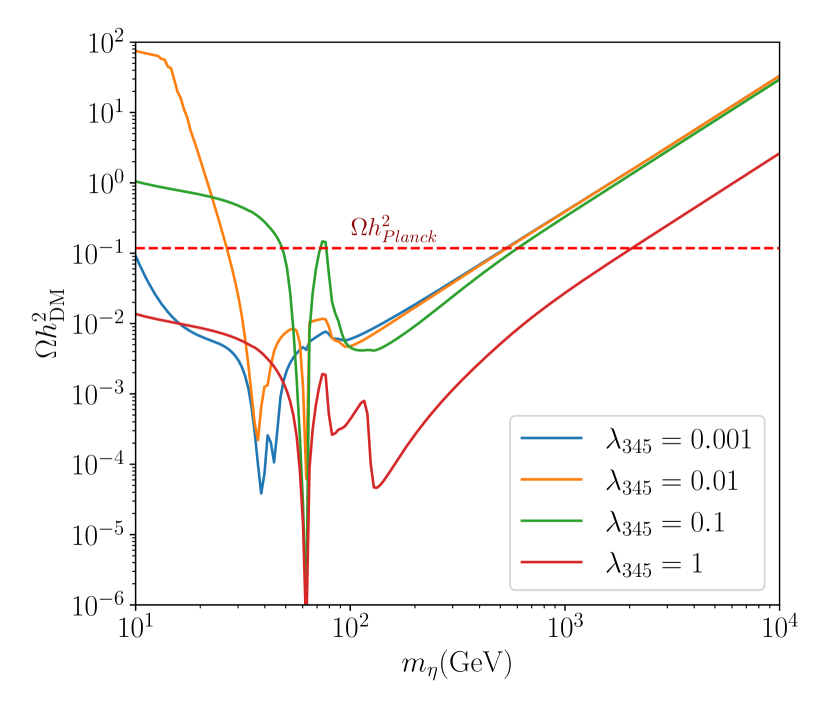
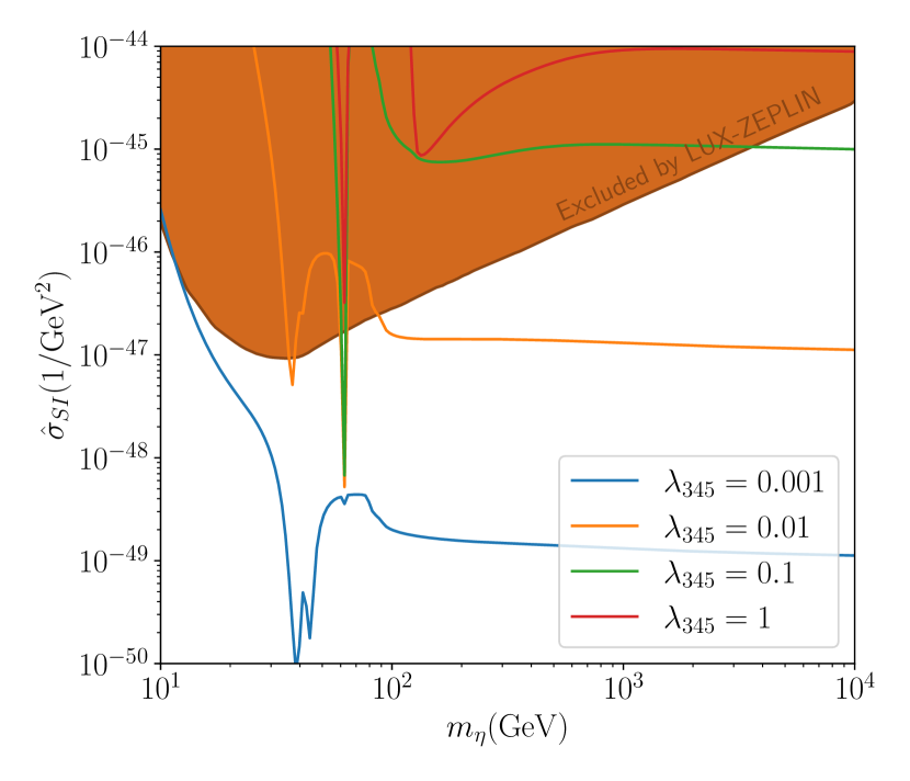
To avoid the overproduction of dark matter, a large needs to be compensated by large scalar couplings, which are constrained by direct detection. However, the direct detection bounds can be evaded if there are cancellations between and in ; in this case, the strongest constraint comes from the requirement of perturbativity. Combining both constraints, we find that must lie between around and to be able to produce the correct relic abundance.
VI Finding the Joint Parameter Space
The present model has the following free parameters: the Yukawa matrix , the masses , and the scalar couplings . Since the Yukawa matrix, and therefore the neutrino mass matrix, has rank two, we can reduce the neutrino mass matrix to a matrix, which, in the neutrino mass eigenbasis, is given by
| (40) |
where we define
| (41) |
For fixed Yukawa matrix and particle masses, we can invert relation Eq. 40 to obtain
| (42) |
with .
The lepton asymmetry is produced in two lepton flavors with opposite signs. We therefore need different washout rates , otherwise the asymmetries would exactly cancel, and the final asymmetry is maximized in the strongly hierarchical case . In addition to this, the mass splitting between the two neutral components is proportional to Re per Eq. 12, which we also want to maximize, in order to avoid the direct detection via -boson exchange. We further choose Re. We find that setting and arbitrary, we maximize the -violating phase and obtain .
For scanning the parameter space, we fix and . Furthermore, since the impact of the Yukawa couplings to on the equilibration and washout rates are negligible, they are arbitrary. For illustrative purposes, we set . Increasing this ratio can lead to Leptogenesis scales down to , but even ratios down to give an allowed parameter region. The parameter scan with the relevant constraints is shown in Fig. 5.
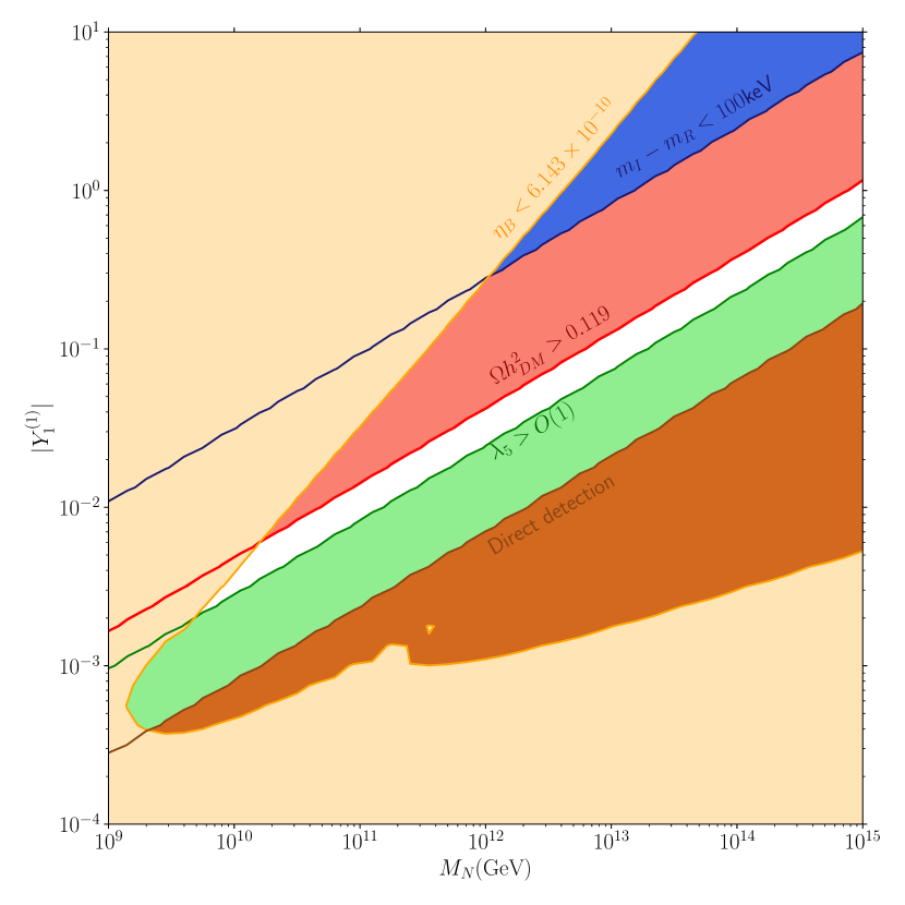
We find there is a region, albeit small, of values consistent with all bounds. Except for the baryon asymmetry, all bounds follow similar curves, which essentially depend on . From Equations 6, 41 and 42, we see that decreasing and increasing leads to an increase in . Small values of are constrained first because this would lead to DM overproduction (red region) and a small mass splitting between and , making it susceptible to direct detection via neutral currents, while large values of would violate perturbativity and would be inconsistent with direct detection bounds.
VII Experimental Signatures
As discussed in Section III, the main experimental constraints come from lepton flavor violation and direct detection experiments. Due to the very large mass of , lepton flavor violating processes are strongly suppressed, and an improvement of many orders of magnitude in LFV precision measurements is required before a signal from our model is expected. On the other hand, we find that LUX-ZEPLIN places stringent bounds on the scalar couplings of the new doublets. While, as we have argued in Section V, detection can be avoided in case of cancellations between and , large cancellations would require severe fine-tuning.
A third detection prospect is via missing transverse energy in collider experiments. For these searches, our model has essentialy the same signatures as the inert Higgs doublet model, whose main detection channels for collider searches include: mono-jet production (), mono- production (), mono-Higgs production ( and ) and vector boson fusion () for hadron colliders as well as and for electron-positron colliders [94, 97, 98, 99, 100, 101, 102, 101, 103, 104, 105, 106]. It was found that masses up to can be probed at the HL-LHC [101, 103, 104], which, while unable to explain all of the dark matter within our model, is also a viable scenario. This can be improved with higher center-of-mass energies, for instance in ILC or CLIC, which can potentially probe masses up to [105, 106].
VIII Conclusion
In this work we have investigated the simultaneous neutrino mass generation, DM production, and Leptogenesis from a minimal realization of the Scotogenic model, with two additional scalar doublets and a single Majorana fermion only, odd under a symmetry.
The Leptogenesis mechanism we consider is via heavy Majorana fermion decay, where the decay asymmetry arises from the mixing and interferences between the two dark scalars. In our treatment of Leptogenesis we have included an improved estimate of the scalar propagator width which strongly limits the resonant enhancement of the asymmetry. Due to the large width of the propagator, we find that in some regions of the parameter space vertex contributions to the -violating source term can become more relevant than the resonant wavefunction contributions. We also find that, on the one hand, large quartic couplings for the new scalars are needed to avoid the overproduction of dark matter, while on the other hand, direct detection experiments place stringent bounds on these quartic couplings, which can only be evaded if some cancellation between the scalar couplings occurs.
Nevertheless, performing a scan of and of the Yukawa couplings, for we find a region of parameter space consistent with all constraints, which could explain the neutrino masses, account for the dark matter and the baryon asymmetry of the Universe simultaneously. Since there is a single Majorana fermion in the model, the -violating processes differ substantially from those in standard Leptogenesis. In particular, these involve the interference of new particles that, while in the dark sector, are not Standard Model singlets. In the future, it may be interesting to pursue similar possibilities more broadly.
Acknowledgements
EW’s work is supported by the Collaborative Research Center SFB 1258 of the German Research Foundation. We would also like to thank Carlos Tamarit for useful discussions.
Appendix A Kinetic Equilibration of the Propagator
In order for Eq. 19 to hold, kinetic equilibrium has to be established for the scalar doublets . Since is out of equilibrium, drives also out of equilibrium. Since we do not make assumptions about the distribution of , it is not immediately clear why can still be taken to be of the form of a kinetic equilibrium distribution. This approximation, which is often used for calculations in different scenarios for baryogenesis, shall be justified in the present appendix. From the kinetic equations for the resummed scalar propagator we have [86, 87]
| (43) |
In the current discussion, we only include contributions to the self-energy from Yukawa and gauge interactions, and respectively. For the moment, consider the case where , so that the scalar particles are degenerate in their masses and interactions and that there are only gauge interactions. Looking for stationary solutions, Eq. 43 then reduces to
| (44) |
This can be solved by assuming that the propagators follow a kinetic equilibrium distribution, writing, as in Ref. [88],
| (45a) | ||||
| (45b) | ||||
with
| (46) |
where we have introduced a matrix of chemical potentials . With this we obtain a generalized Kubo-Matrin-Schwinger (KMS) relation for the propagators in kinetic equilibrium
| (47) |
To see that Eqs. (45) hold, note that the self-energy contribution from gauge interactions is given by
| (48) |
where are CTP indices, are flavor indices and is the full gauge boson propagator. Since is in thermal equilibrium, it also observes the KMS relation. We then find that
| (49) |
where the last equality follows from the fact that and commute. With this we find
| (50) |
and verify that Eq. 44 is indeed satisfied. To first order in the chemical potentials, we can approximate
| (51) |
We now restrict the discussion to the components of the propagator accounting for mixing of the scalar flavors, i.e. . The kinetic equation for this part of the propagator is
| (52) |
with the stationary solution
| (53) |
While contains , does not, since to leading order it only entails a fermion loop. Defining
| (54) |
we can rewrite the kinetic equation as
| (55) |
We now define and insert the form of the propagators given in Eqs. (45). We then find that Eq. 55 takes the form
| (56) |
where we have introduced the short-hand notation
| (57a) | ||||
| (57b) | ||||
| (57c) | ||||
| (57d) | ||||
The subscripts here indicate the dependence on , i.e. whether the terms on the right-hand side of Eq. 56 are independent of and if they are dependent, whether they are diagonal or generally nondiagonal in .
When we discretize the momentum , we obtain
| (58) |
which we can interpret as a matrix equation
| (59) |
where is a new expansion parameter which we tag to all quantities driving the distribution out of equilibrium.
Quasi-degenerate case
Here, the mass splitting as well as the interactions mediated by are small compared to the gauge interactions mediated by . The latter thus have time to establish kinetic equilibrium also in the off-diagonal correlations. We thus decompose as
| (60) | ||||
| (61) |
Clearly, the solution to Eq. 59 is
| (62) |
We also recover the pure gauge scenario when we send , in which case Eq. 59 becomes
| (63) |
whose solution is precisely the chemical equilibrium distribution , as we have seen before. From this equation we also recognize that is singular. Then, following Ref. [107], we can regard as a matrix function in and expand as a Laurent series in
| (64) |
where is the order of the pole at . We expect the kernel of to be one-dimensional, and if it is not simultaneously the kernel of , using the method introduced in Ref. [108], we find that has a simple pole at the origin, and from the condition
| (65) |
we obtain the fundamental equations
| (66a) | ||||
| (66b) | ||||
| (66c) | ||||
With these equations, we can find and write our problem as
| (67) |
To zeroth order in , the solution Eq. 62 is given by , but from Eq. 66a, we know that , which means that lies in the kernel of . Since the kernel of is one-dimensional, this implies that is proportional to , and therefore, if the gauge interactions are much stronger than the Yukawa interactions and the squared mass difference of the , can indeed be approximated by , the kinetic equilibrium distribution.
Non-degenerate case
So far we have treated the mass splitting as a perturbation compared to the gauge self-energies. We now want to treat the case where the mass splitting dominates the kinetic equation. The gauge interactions then do not have time to impose kinetic equilibrium on the off-diagonal correlations induced by the out-of-equilibrium Majorana fermion. In this case, we can rewrite Eq. 59 as
| (68) |
where
| (69) | ||||
| (70) |
We can divide Eq. 68 by and obtain
| (71) |
with the solution
| (72) |
Since we assume , we can write as a Neumann series
| (73) |
Since higher order terms are suppressed by powers of , we can keep only the leading order term, which gives us
| (74) |
Going back to Eq. 53, this means we can approximate
| (75) |
If we parametrize the deviation of from equilibrium with a pseudo-chemical potential , we find again a KMS relation for :
| (76) |
from which we can rewrite Eq. 75 as
| (77) |
where we have omitted the contribution from since we assume to be much heavier than , and can therefore neglect its on-shell contribution. To first order in the chemical potential we can write
| (78) |
In the regime of interest, , the dominant contributions arise for and , so that we can neglect the dependence of and rewrite this as
| (79) |
where we have introduced a new chemical potential , chosen in such a way that both definitions produce the same charges. So we can again apply Eq. 19. Note that while the approximation does not apply in the exponential tail, it holds for the relevant momentum range.
With this we have shown that we can parametrize with a chemical potential both in the case where the kinetic equation (43) is dominated by gauge (or other) interactions driving it to kinetic equilibrium as well as when it is dominated by the mass splitting.
Appendix B Spectral Self-Energies
To determine the width of the mixed scalar propagator from the kinetic equation (18), we need to compute the spectral self-energies for the fields. The two main contributions come from the Yukawa and the gauge interactions. In Eq. 21 we have introduced the averaged rates, which are defined as
| (80) | ||||
| (81) | ||||
| (82) | ||||
| (83) |
Using CTP methods and assuming , we find [3]
| (84) |
where is a chemical potential we introduce to parametrize the deviation of from equilibrium. The Yukawa spectral self-energy can be computed at first order, giving
| (85) |
where we have approximated the distribution of the Majorana neutrinos as nonrelativistic. We then find
| (86) |
Defining the reduced cross section for a two-body scattering as
| (87) |
where is the usual cross-section and is the function
| (88) |
one can compute the reaction density as
| (89) |
We present here a detailed derivation of , which, to the best of our knowledge, is computed for the first time. The relevant contribution to the self-energy comes from the sunset diagram and is given by
| (90) |
where stands for the coupling structure and the sum is over the field configurations running in the loop. We also choose a signature where all temporal momenta have the same sign (since the expression is symmetric under exchange of the momenta, this can always be done). The collision term is then
| (91) | ||||
While also contributes wherever appears, this would be a higher order correction, which we discard as we only consider linear terms in the off-diagonal correlations of the particles . Similarly, also should contribute where appears, but since we assume diagonal propagators to be in equilibrium, this would give a purely equilibrium, and therefore vanishing, contribution. Since , we can also neglect contributions, since they are strongly Maxwell-suppressed. Lastly, we see that not only appears in the collision term but also , implying that there is some mixing between and . We also neglect this term to avoid complicating the problem even further. The full reaction rate is obtained by integrating the collision term over , and, in spite of the complicated flavor structure, we can approximate all processes as having the same kinematics. Paying particular attention to the signs of the contributions, this gives us
| (92) | ||||
where we divide by two to average over the degrees of freedom, and
| (93) | ||||
in Boltzmann approximation. Then, with the approximation that all particles have the same reaction rate regardless of momentum, we can write [3]
| (94) |
As for gauge interactions, since we are in a regime where the gauge bosons are massless, the first-order self-energy corresponding to processes vanishes. We therefore need to go to second order, which corresponds to two-by-two scatterings. The only relevant scatterings are pair creation and annihilation since they are the only ones that can change particle number. We use FeynArts [109] to generate the relevant diagrams and FeynCalc [110, 111, 112] to obtain the corresponding amplitudes. As opposed to earlier estimates from Ref. [3], IR divergences in and -channel cancel, and these contributions can be directly accounted for. The total reduced cross-section we find is
| (95) |
from which we obtain the reaction density
| (96) |
From this, following Ref. [3], using and we find
| (97) |
which is one order of magnitude larger than the expression in Ref. [3].
Appendix C Vertex Contribution to the Source Term
The vertex contribution to the -source is given by
| (98) | ||||
Dropping on-shell terms, we have
| (99) | ||||
where we have used for off-shell .
As was argued in Ref. [89], we only need to keep the absorptive parts of and , since the dispersive parts cancel upon integration. We then have
We can use the spatial delta functions to carry out the and the integrals. Neglecting quantum statistical factors, we then have
We can use spherical coordinates to express and with respect to through the angles and use the delta functions to do the integrals. Approximating , we have
We express
The first term vanishes when performing the integrals, and we are left with
Since we assume , we can approximate
| (100) |
With this we can evaluate the above integral and obtain
| (101) |
Dividing by
| (102) |
and shifting to comoving coordinates, we find
| (103) |
References
- Fukugita and Yanagida [1986] M. Fukugita and T. Yanagida, Baryogenesis Without Grand Unification, Phys. Lett. B 174, 45 (1986).
- Garbrecht [2012] B. Garbrecht, Leptogenesis from Additional Higgs Doublets, Phys. Rev. D 85, 123509 (2012), arXiv:1201.5126 [hep-ph] .
- Garbrecht [2013] B. Garbrecht, Baryogenesis from Mixing of Lepton Doublets, Nucl. Phys. B 868, 557 (2013), arXiv:1210.0553 [hep-ph] .
- Hagedorn et al. [2018] C. Hagedorn, J. Herrero-García, E. Molinaro, and M. A. Schmidt, Phenomenology of the Generalised Scotogenic Model with Fermionic Dark Matter, JHEP 11, 103, arXiv:1804.04117 [hep-ph] .
- Kumar et al. [2020] N. Kumar, T. Nomura, and H. Okada, Scotogenic neutrino mass with large multiplet fields, Eur. Phys. J. C 80, 801 (2020), arXiv:1912.03990 [hep-ph] .
- Escribano et al. [2020] P. Escribano, M. Reig, and A. Vicente, Generalizing the Scotogenic model, JHEP 07, 097, arXiv:2004.05172 [hep-ph] .
- Leite et al. [2020] J. Leite, A. Morales, J. W. F. Valle, and C. A. Vaquera-Araujo, Dark matter stability from Dirac neutrinos in scotogenic 3-3-1-1 theory, Phys. Rev. D 102, 015022 (2020), arXiv:2005.03600 [hep-ph] .
- Sarazin et al. [2021] M. Sarazin, J. Bernigaud, and B. Herrmann, Dark matter and lepton flavour phenomenology in a singlet-doublet scotogenic model, JHEP 12, 116, arXiv:2107.04613 [hep-ph] .
- Ahriche [2023] A. Ahriche, A scotogenic model with two inert doublets, JHEP 02, 028, arXiv:2208.00500 [hep-ph] .
- Alvarez et al. [2023] A. Alvarez, A. Banik, R. Cepedello, B. Herrmann, W. Porod, M. Sarazin, and M. Schnelke, Accommodating muon (g 2) and leptogenesis in a scotogenic model, JHEP 06, 163, arXiv:2301.08485 [hep-ph] .
- Bonilla et al. [2023] C. Bonilla, A. E. Carcamo Hernandez, J. Goncalves, V. K. N., A. P. Morais, and R. Pasechnik, Gravitational waves from a scotogenic two-loop neutrino mass model, (2023), arXiv:2305.01964 [hep-ph] .
- Escribano et al. [2023] P. Escribano, V. M. Lozano, and A. Vicente, Scotogenic explanation for the 95 GeV excesses, Phys. Rev. D 108, 115001 (2023), arXiv:2306.03735 [hep-ph] .
- Karan et al. [2023] A. Karan, S. Sadhukhan, and J. W. F. Valle, Phenomenological profile of scotogenic fermionic dark matter, JHEP 12, 185, arXiv:2308.09135 [hep-ph] .
- Maniatis et al. [2006] M. Maniatis, A. von Manteuffel, O. Nachtmann, and F. Nagel, Stability and symmetry breaking in the general two-Higgs-doublet model, Eur. Phys. J. C 48, 805 (2006), arXiv:hep-ph/0605184 .
- Keus et al. [2014a] V. Keus, S. F. King, and S. Moretti, Three-Higgs-doublet models: symmetries, potentials and Higgs boson masses, JHEP 01, 052, arXiv:1310.8253 [hep-ph] .
- Li et al. [2014] X.-Q. Li, J. Lu, and A. Pich, Decays in the Aligned Two-Higgs-Doublet Model, JHEP 06, 022, arXiv:1404.5865 [hep-ph] .
- Maniatis and Nachtmann [2015] M. Maniatis and O. Nachtmann, Stability and symmetry breaking in the general three-Higgs-doublet model, JHEP 02, 058, [Erratum: JHEP 10, 149 (2015)], arXiv:1408.6833 [hep-ph] .
- Chen and Nomura [2014] C.-H. Chen and T. Nomura, Two-Higgs-Doublet Type-II Seesaw Model, Phys. Rev. D 90, 075008 (2014), arXiv:1406.6814 [hep-ph] .
- Abbas et al. [2015] G. Abbas, A. Celis, X.-Q. Li, J. Lu, and A. Pich, Flavour-changing top decays in the aligned two-Higgs-doublet model, JHEP 06, 005, arXiv:1503.06423 [hep-ph] .
- Maniatis et al. [2015] M. Maniatis, D. Mehta, and C. M. Reyes, Stability and symmetry breaking in a three-Higgs-doublet model with lepton family symmetry O(2), Phys. Rev. D 92, 035017 (2015), arXiv:1503.05948 [hep-ph] .
- Han et al. [2016] T. Han, S. K. Kang, and J. Sayre, Muon in the aligned two Higgs doublet model, JHEP 02, 097, arXiv:1511.05162 [hep-ph] .
- Hu et al. [2017a] Q.-Y. Hu, X.-Q. Li, and Y.-D. Yang, decay in the Aligned Two-Higgs-Doublet Model, Eur. Phys. J. C 77, 190 (2017a), arXiv:1612.08867 [hep-ph] .
- Hu et al. [2017b] Q.-Y. Hu, X.-Q. Li, and Y.-D. Yang, The decay in the aligned two-Higgs-doublet model, Eur. Phys. J. C 77, 228 (2017b), arXiv:1701.04029 [hep-ph] .
- Abbas et al. [2018] G. Abbas, D. Das, and M. Patra, Loop induced decays in the aligned two-Higgs-doublet model, Phys. Rev. D 98, 115013 (2018), arXiv:1806.11035 [hep-ph] .
- Cogollo et al. [2019] D. Cogollo, R. D. Matheus, T. B. de Melo, and F. S. Queiroz, Type I + II Seesaw in a Two Higgs Doublet Model, Phys. Lett. B 797, 134813 (2019), arXiv:1904.07883 [hep-ph] .
- Jurčiukonis et al. [2019] D. Jurčiukonis, T. Gajdosik, and A. Juodagalvis, Seesaw neutrinos with one right-handed singlet field and a second Higgs doublet, JHEP 11, 146, arXiv:1909.00752 [hep-ph] .
- Chen et al. [2021a] C.-H. Chen, C.-W. Chiang, and T. Nomura, Muon g-2 in a two-Higgs-doublet model with a type-II seesaw mechanism, Phys. Rev. D 104, 055011 (2021a), arXiv:2104.03275 [hep-ph] .
- Wang [2021] S.-W. Wang, Study of Decay in the Aligned Two-Higgs-Doublet Model and Vector Leptoquark Model, Int. J. Theor. Phys. 60, 3225 (2021).
- Enomoto et al. [2022] K. Enomoto, S. Kanemura, and Y. Mura, New benchmark scenarios of electroweak baryogenesis in aligned two Higgs double models, JHEP 09, 121, arXiv:2207.00060 [hep-ph] .
- Sartore et al. [2022] L. Sartore, M. Maniatis, I. Schienbein, and B. Herrmann, The general Two-Higgs Doublet Model in a gauge-invariant form, JHEP 12, 051, arXiv:2208.13719 [hep-ph] .
- Cai et al. [2022] F.-M. Cai, S. Funatsu, X.-Q. Li, and Y.-D. Yang, Rare top-quark decays in the aligned two-Higgs-doublet model, Eur. Phys. J. C 82, 881 (2022), arXiv:2202.08091 [hep-ph] .
- Connell et al. [2023] J. M. Connell, P. Ferreira, and H. E. Haber, Accommodating hints of new heavy scalars in the framework of the flavor-aligned two-Higgs-doublet model, Phys. Rev. D 108, 055031 (2023), arXiv:2302.13697 [hep-ph] .
- Karan et al. [2024] A. Karan, V. Miralles, and A. Pich, Updated global fit of the aligned two-Higgs-doublet model with heavy scalars, Phys. Rev. D 109, 035012 (2024), arXiv:2307.15419 [hep-ph] .
- Darvishi et al. [2023] N. Darvishi, A. Pilaftsis, and J.-H. Yu, Maximising CP Violation in Naturally Aligned Two-Higgs Doublet Models, (2023), arXiv:2312.00882 [hep-ph] .
- Arcadi and Khan [2023] G. Arcadi and S. Khan, Axion Dark Matter and additional BSM aspects in an extended 2HDM setup, (2023), arXiv:2312.17099 [hep-ph] .
- Machado and Pleitez [2016] A. C. B. Machado and V. Pleitez, A model with two inert scalar doublets, Annals Phys. 364, 53 (2016), arXiv:1205.0995 [hep-ph] .
- Fortes et al. [2015] E. C. F. S. Fortes, A. C. B. Machado, J. Montaño, and V. Pleitez, Scalar dark matter candidates in a two inert Higgs doublet model, J. Phys. G 42, 105003 (2015), arXiv:1407.4749 [hep-ph] .
- Keus et al. [2014b] V. Keus, S. F. King, S. Moretti, and D. Sokolowska, Dark Matter with Two Inert Doublets plus One Higgs Doublet, JHEP 11, 016, arXiv:1407.7859 [hep-ph] .
- Keus et al. [2014c] V. Keus, S. F. King, and S. Moretti, Phenomenology of the inert ( 2+1 ) and ( 4+2 ) Higgs doublet models, Phys. Rev. D 90, 075015 (2014c), arXiv:1408.0796 [hep-ph] .
- Alanne et al. [2016] T. Alanne, K. Kainulainen, K. Tuominen, and V. Vaskonen, Baryogenesis in the two doublet and inert singlet extension of the Standard Model, JCAP 08, 057, arXiv:1607.03303 [hep-ph] .
- Aranda et al. [2021] A. Aranda, D. Hernández-Otero, J. Hernández-Sanchez, V. Keus, S. Moretti, D. Rojas-Ciofalo, and T. Shindou, Z3 symmetric inert ( 2+1 )-Higgs-doublet model, Phys. Rev. D 103, 015023 (2021), arXiv:1907.12470 [hep-ph] .
- Merchand and Sher [2020] M. Merchand and M. Sher, Constraints on the Parameter Space in an Inert Doublet Model with two Active Doublets, JHEP 03, 108, arXiv:1911.06477 [hep-ph] .
- Belanger et al. [2022] G. Belanger, A. Mjallal, and A. Pukhov, WIMP and FIMP dark matter in the inert doublet plus singlet model, Phys. Rev. D 106, 095019 (2022), arXiv:2205.04101 [hep-ph] .
- Khojali et al. [2022] M. O. Khojali, A. Abdalgabar, A. Ahriche, and A. S. Cornell, Dark matter in a singlet-extended inert Higgs-doublet model, Phys. Rev. D 106, 095039 (2022), arXiv:2206.06211 [hep-ph] .
- Singirala et al. [2023] S. Singirala, D. K. Singha, and R. Mohanta, Neutrino magnetic moment and inert doublet dark matter in a Type-III radiative scenario, Phys. Rev. D 108, 095048 (2023), arXiv:2306.14801 [hep-ph] .
- Angel et al. [2013] P. W. Angel, Y. Cai, N. L. Rodd, M. A. Schmidt, and R. R. Volkas, Testable two-loop radiative neutrino mass model based on an effective operator, JHEP 10, 118, [Erratum: JHEP 11, 092 (2014)], arXiv:1308.0463 [hep-ph] .
- Addazi [2015] A. Addazi, ‘Exotic vector-like pair’ of color-triplet scalars, JHEP 04, 153, arXiv:1501.04660 [hep-ph] .
- Addazi and Bianchi [2015] A. Addazi and M. Bianchi, Un-oriented Quiver Theories for Majorana Neutrons, JHEP 07, 144, arXiv:1502.01531 [hep-ph] .
- Carquin et al. [2019] E. Carquin, N. A. Neill, J. C. Helo, and M. Hirsch, Exotic colored fermions and lepton number violation at the LHC, Phys. Rev. D 99, 115028 (2019), arXiv:1904.07257 [hep-ph] .
- Dvali [1992] G. R. Dvali, Can ’doublet - triplet splitting’ problem be solved without doublet - triplet splitting?, Phys. Lett. B 287, 101 (1992).
- Dvali [1996] G. R. Dvali, Light color triplet Higgs is compatible with proton stability: An Alternative approach to the doublet - triplet splitting problem, Phys. Lett. B 372, 113 (1996), arXiv:hep-ph/9511237 .
- Kawamura [2001] Y. Kawamura, Triplet doublet splitting, proton stability and extra dimension, Prog. Theor. Phys. 105, 999 (2001), arXiv:hep-ph/0012125 .
- von Gersdorff [2021] G. von Gersdorff, A Clockwork Solution to the Doublet-Triplet Splitting Problem, Phys. Lett. B 813, 136039 (2021), arXiv:2009.08480 [hep-ph] .
- Pilaftsis [2000] A. Pilaftsis, Loop induced CP violation in the gaugino and Higgsino sectors of supersymmetric theories, Phys. Rev. D 62, 016007 (2000), arXiv:hep-ph/9912253 .
- Choi et al. [2001] S. Y. Choi, M. Drees, B. Gaissmaier, and J. S. Lee, CP violation in tau slepton pair production at muon colliders, Phys. Rev. D 64, 095009 (2001), arXiv:hep-ph/0103284 .
- Li et al. [2008] Y. Li, S. Profumo, and M. Ramsey-Musolf, Higgs-Higgsino-Gaugino Induced Two Loop Electric Dipole Moments, Phys. Rev. D 78, 075009 (2008), arXiv:0806.2693 [hep-ph] .
- Kim et al. [2009a] S. G. Kim, N. Maekawa, A. Matsuzaki, K. Sakurai, and T. Yoshikawa, CP asymmetries of and in SUSY GUT Model with Non-universal Sfermion Masses, Prog. Theor. Phys. 121, 49 (2009a), arXiv:0803.4250 [hep-ph] .
- Kim et al. [2009b] S.-G. Kim, N. Maekawa, K. I. Nagao, M. M. Nojiri, and K. Sakurai, LHC signature of supersymmetric models with non-universal sfermion masses, JHEP 10, 005, arXiv:0907.4234 [hep-ph] .
- Cheung et al. [2009] K. Cheung, S. Y. Choi, and J. Song, Impact on the Light Higgsino-LSP Scenario from Physics beyond the Minimal Supersymmetric Standard Model, Phys. Lett. B 677, 54 (2009), arXiv:0903.3175 [hep-ph] .
- Baer et al. [2011] H. Baer, V. Barger, and P. Huang, Hidden SUSY at the LHC: the light higgsino-world scenario and the role of a lepton collider, JHEP 11, 031, arXiv:1107.5581 [hep-ph] .
- Sakurai and Takayama [2011] K. Sakurai and K. Takayama, Constraint from recent ATLAS results to non-universal sfermion mass models and naturalness, JHEP 12, 063, arXiv:1106.3794 [hep-ph] .
- Kozaczuk et al. [2012] J. Kozaczuk, S. Profumo, M. J. Ramsey-Musolf, and C. L. Wainwright, Supersymmetric Electroweak Baryogenesis Via Resonant Sfermion Sources, Phys. Rev. D 86, 096001 (2012), arXiv:1206.4100 [hep-ph] .
- Altmannshofer et al. [2013] W. Altmannshofer, R. Harnik, and J. Zupan, Low Energy Probes of PeV Scale Sfermions, JHEP 11, 202, arXiv:1308.3653 [hep-ph] .
- Nagata and Shirai [2014] N. Nagata and S. Shirai, Sfermion Flavor and Proton Decay in High-Scale Supersymmetry, JHEP 03, 049, arXiv:1312.7854 [hep-ph] .
- Kim and Ray [2015] J. S. Kim and T. S. Ray, The higgsino-singlino world at the large hadron collider, Eur. Phys. J. C 75, 40 (2015), arXiv:1405.3700 [hep-ph] .
- Maekawa et al. [2017] N. Maekawa, Y. Muramatsu, and Y. Shigekami, Constraints of chromoelectric dipole moments to natural SUSY type sfermion spectrum, Phys. Rev. D 95, 115021 (2017), arXiv:1702.01527 [hep-ph] .
- Krall and Reece [2018] R. Krall and M. Reece, Last Electroweak WIMP Standing: Pseudo-Dirac Higgsino Status and Compact Stars as Future Probes, Chin. Phys. C 42, 043105 (2018), arXiv:1705.04843 [hep-ph] .
- Arcadi et al. [2023] G. Arcadi, A. Djouadi, H.-J. He, J.-L. Kneur, and R.-Q. Xiao, The hMSSM with a light gaugino/higgsino sector: implications for collider and astroparticle physics, JHEP 05, 095, arXiv:2206.11881 [hep-ph] .
- Shafi et al. [2023] Q. Shafi, A. Tiwari, and C. S. Un, Third family quasi-Yukawa unification: Higgsino dark matter, NLSP gluino, and all that, Phys. Rev. D 108, 035027 (2023), arXiv:2302.02905 [hep-ph] .
- Ma [2006a] E. Ma, Verifiable radiative seesaw mechanism of neutrino mass and dark matter, Phys. Rev. D 73, 077301 (2006a), arXiv:hep-ph/0601225 .
- Ma [2006b] E. Ma, Common origin of neutrino mass, dark matter, and baryogenesis, Mod. Phys. Lett. A 21, 1777 (2006b), arXiv:hep-ph/0605180 .
- Hehn and Ibarra [2013] D. Hehn and A. Ibarra, A radiative model with a naturally mild neutrino mass hierarchy, Phys. Lett. B 718, 988 (2013), arXiv:1208.3162 [hep-ph] .
- Baumholzer et al. [2018] S. Baumholzer, V. Brdar, and P. Schwaller, The New MSM (MSM): Radiative Neutrino Masses, keV-Scale Dark Matter and Viable Leptogenesis with sub-TeV New Physics, JHEP 08, 067, arXiv:1806.06864 [hep-ph] .
- Chen et al. [2021b] S.-L. Chen, A. Dutta Banik, and Z.-K. Liu, Common origin of radiative neutrino mass, dark matter and leptogenesis in scotogenic Georgi-Machacek model, Nucl. Phys. B 966, 115394 (2021b), arXiv:2011.13551 [hep-ph] .
- Sarma et al. [2021] L. Sarma, P. Das, and M. K. Das, Scalar dark matter and leptogenesis in the minimal scotogenic model, Nucl. Phys. B 963, 115300 (2021), arXiv:2004.13762 [hep-ph] .
- Mahanta and Borah [2019] D. Mahanta and D. Borah, Fermion dark matter with leptogenesis in minimal scotogenic model, JCAP 11, 021, arXiv:1906.03577 [hep-ph] .
- Borah et al. [2019] D. Borah, P. S. B. Dev, and A. Kumar, TeV scale leptogenesis, inflaton dark matter and neutrino mass in a scotogenic model, Phys. Rev. D 99, 055012 (2019), arXiv:1810.03645 [hep-ph] .
- Suematsu [2024] D. Suematsu, Right-handed neutrino as a common mother of baryon number asymmetry and dark matter, (2024), arXiv:2402.10561 [hep-ph] .
- Toma and Vicente [2014] T. Toma and A. Vicente, Lepton Flavor Violation in the Scotogenic Model, JHEP 01, 160, arXiv:1312.2840 [hep-ph] .
- Workman [2022] R. L. Workman (Particle Data Group), Review of Particle Physics, PTEP 2022, 083C01 (2022).
- Barbieri et al. [2006] R. Barbieri, L. J. Hall, and V. S. Rychkov, Improved naturalness with a heavy Higgs: An Alternative road to LHC physics, Phys. Rev. D 74, 015007 (2006), arXiv:hep-ph/0603188 .
- Barbieri et al. [1989] R. Barbieri, M. Frigeni, and G. F. Giudice, Dark Matter Neutralinos in Supergravity Theories, Nucl. Phys. B 313, 725 (1989).
- Aalbers et al. [2023] J. Aalbers et al. (LZ), First Dark Matter Search Results from the LUX-ZEPLIN (LZ) Experiment, Phys. Rev. Lett. 131, 041002 (2023), arXiv:2207.03764 [hep-ex] .
- Klimenko [1985] K. G. Klimenko, Conditions for certain higgs potentials to be bounded below, Theor. Math. Phys.; (United States) 62:1, 10.1007/BF01034825 (1985).
- Branco et al. [2012] G. C. Branco, P. M. Ferreira, L. Lavoura, M. N. Rebelo, M. Sher, and J. P. Silva, Theory and phenomenology of two-Higgs-doublet models, Phys. Rept. 516, 1 (2012), arXiv:1106.0034 [hep-ph] .
- Garbrecht and Herranen [2012] B. Garbrecht and M. Herranen, Effective Theory of Resonant Leptogenesis in the Closed-Time-Path Approach, Nucl. Phys. B 861, 17 (2012), arXiv:1112.5954 [hep-ph] .
- Garny et al. [2013] M. Garny, A. Kartavtsev, and A. Hohenegger, Leptogenesis from first principles in the resonant regime, Annals Phys. 328, 26 (2013), arXiv:1112.6428 [hep-ph] .
- Beneke et al. [2011] M. Beneke, B. Garbrecht, C. Fidler, M. Herranen, and P. Schwaller, Flavoured Leptogenesis in the CTP Formalism, Nucl. Phys. B 843, 177 (2011), arXiv:1007.4783 [hep-ph] .
- Beneke et al. [2010] M. Beneke, B. Garbrecht, M. Herranen, and P. Schwaller, Finite Number Density Corrections to Leptogenesis, Nucl. Phys. B 838, 1 (2010), arXiv:1002.1326 [hep-ph] .
- Buchmuller et al. [2005] W. Buchmuller, P. Di Bari, and M. Plumacher, Leptogenesis for pedestrians, Annals Phys. 315, 305 (2005), arXiv:hep-ph/0401240 .
- Harvey and Turner [1990] J. A. Harvey and M. S. Turner, Cosmological baryon and lepton number in the presence of electroweak fermion number violation, Phys. Rev. D 42, 3344 (1990).
- Chung et al. [2009] D. J. H. Chung, B. Garbrecht, and S. Tulin, The Effect of the Sparticle Mass Spectrum on the Conversion of B-L to B, JCAP 03, 008, arXiv:0807.2283 [hep-ph] .
- Aghanim et al. [2020] N. Aghanim et al. (Planck), Planck 2018 results. VI. Cosmological parameters, Astron. Astrophys. 641, A6 (2020), [Erratum: Astron.Astrophys. 652, C4 (2021)], arXiv:1807.06209 [astro-ph.CO] .
- Belyaev et al. [2018] A. Belyaev, G. Cacciapaglia, I. P. Ivanov, F. Rojas-Abatte, and M. Thomas, Anatomy of the Inert Two Higgs Doublet Model in the light of the LHC and non-LHC Dark Matter Searches, Phys. Rev. D 97, 035011 (2018), arXiv:1612.00511 [hep-ph] .
- Alloul et al. [2014] A. Alloul, N. D. Christensen, C. Degrande, C. Duhr, and B. Fuks, FeynRules 2.0 - A complete toolbox for tree-level phenomenology, Comput. Phys. Commun. 185, 2250 (2014), arXiv:1310.1921 [hep-ph] .
- Belanger et al. [2014] G. Belanger, F. Boudjema, A. Pukhov, and A. Semenov, micrOMEGAs3: A program for calculating dark matter observables, Comput. Phys. Commun. 185, 960 (2014), arXiv:1305.0237 [hep-ph] .
- Poulose et al. [2017] P. Poulose, S. Sahoo, and K. Sridhar, Exploring the Inert Doublet Model through the dijet plus missing transverse energy channel at the LHC, Phys. Lett. B 765, 300 (2017), arXiv:1604.03045 [hep-ph] .
- Ávila et al. [2020] I. M. Ávila, V. De Romeri, L. Duarte, and J. W. F. Valle, Phenomenology of scotogenic scalar dark matter, Eur. Phys. J. C 80, 908 (2020), arXiv:1910.08422 [hep-ph] .
- Belyaev et al. [2019] A. Belyaev, T. R. Fernandez Perez Tomei, P. G. Mercadante, C. S. Moon, S. Moretti, S. F. Novaes, L. Panizzi, F. Rojas, and M. Thomas, Advancing LHC probes of dark matter from the inert two-Higgs-doublet model with the monojet signal, Phys. Rev. D 99, 015011 (2019), arXiv:1809.00933 [hep-ph] .
- Kalinowski et al. [2019] J. Kalinowski, W. Kotlarski, T. Robens, D. Sokolowska, and A. F. Zarnecki, Exploring Inert Scalars at CLIC, JHEP 07, 053, arXiv:1811.06952 [hep-ph] .
- Datta et al. [2017] A. Datta, N. Ganguly, N. Khan, and S. Rakshit, Exploring collider signatures of the inert Higgs doublet model, Phys. Rev. D 95, 015017 (2017), arXiv:1610.00648 [hep-ph] .
- Ghosh et al. [2022] A. Ghosh, P. Konar, and S. Seth, Precise probing of the inert Higgs-doublet model at the LHC, Phys. Rev. D 105, 115038 (2022), arXiv:2111.15236 [hep-ph] .
- Wan et al. [2018] N. Wan, N. Li, B. Zhang, H. Yang, M.-F. Zhao, M. Song, G. Li, and J.-Y. Guo, Searches for Dark Matter via Mono-W Production in Inert Doublet Model at the LHC, Commun. Theor. Phys. 69, 617 (2018).
- Dutta et al. [2018] B. Dutta, G. Palacio, J. D. Ruiz-Alvarez, and D. Restrepo, Vector Boson Fusion in the Inert Doublet Model, Phys. Rev. D 97, 055045 (2018), arXiv:1709.09796 [hep-ph] .
- Kalinowski et al. [2018] J. Kalinowski, W. Kotlarski, T. Robens, D. Sokolowska, and A. F. Zarnecki, Benchmarking the Inert Doublet Model for colliders, JHEP 12, 081, arXiv:1809.07712 [hep-ph] .
- Kalinowski et al. [2020] J. Kalinowski, W. Kotlarski, T. Robens, D. Sokolowska, and A. F. Zarnecki, The Inert Doublet Model at current and future colliders, J. Phys. Conf. Ser. 1586, 012023 (2020), arXiv:1903.04456 [hep-ph] .
- Avrachenkov et al. [2001] K. Avrachenkov, M. Haviv, and P. Howlett, Inversion of analytic matrix functions that are singular at the origin, SIAM Journal on Matrix Analysis and Applications 22 (2001).
- Sain and Massey [1969] M. K. Sain and J. L. Massey, Invertibility of linear time-invariant dynamical systems, IEEE Transactions on Automatic Control 14, 141 (1969).
- Hahn [2001] T. Hahn, Generating Feynman diagrams and amplitudes with FeynArts 3, Comput. Phys. Commun. 140, 418 (2001), arXiv:hep-ph/0012260 .
- Shtabovenko et al. [2020] V. Shtabovenko, R. Mertig, and F. Orellana, FeynCalc 9.3: New features and improvements, Comput. Phys. Commun. 256, 107478 (2020), arXiv:2001.04407 [hep-ph] .
- Shtabovenko et al. [2016] V. Shtabovenko, R. Mertig, and F. Orellana, New Developments in FeynCalc 9.0, Comput. Phys. Commun. 207, 432 (2016), arXiv:1601.01167 [hep-ph] .
- Mertig et al. [1991] R. Mertig, M. Bohm, and A. Denner, FEYN CALC: Computer algebraic calculation of Feynman amplitudes, Comput. Phys. Commun. 64, 345 (1991).