What is to Be Gained by Ensemble Models in Analysis of Spectroscopic Data?

Abstract

An empirical study was carried out to compare different implementations of ensemble models aimed at improving prediction in spectroscopic data. A wide range of candidate models were fitted to benchmark datasets from regression and classification settings. A statistical analysis using linear mixed model was carried out on prediction performance criteria resulting from model fits over random splits of the data. The results showed that the ensemble classifiers were able to consistently outperform candidate models in our application.

Keywords: Chemometrics, Fourier transform mid-infrared spectroscopy, machine learning, milk quality

1 Introduction

Vibrational spectroscopic techniques, including near-infrared (NIR), mid-infrared (MIR), and Raman, use the effect of light to provide information about the constituents of a sample. These low cost, rapid and noninvasive techniques are widely and routinely used in many application domains. Prediction in spectroscopic data is a topic of major interest in chemometric literature, see for example Frizzarin et al., 2021c ; Frizzarin et al., 2021b ; Singh and Domijan, (2019). Numerous advances in statistical machine learning model methodology in the past few decades offer the potential to improve prediction performance over the well-established partial least squares (PLS) approach. Comparative analyses of algorithm prediction ability for spectroscopic data have shown that PLS variants perform strongly Frizzarin et al., 2021b ; Singh and Domijan, (2019), but that there isn’t a single model that will outperform others in all settings. Results are context dependent and specifying only a single model is not the optimal strategy to generate predictions.

Ensemble methods is an umbrella term for model combination techniques to improve prediction accuracy. Ensembles fit multiple candidate machine learning models and combine their predictions in a meta-learner, a second layer model. The idea is that the new ensemble model is more robust as the individual weaknesses and biases of candidate models are offset by the strengths of other candidates.

In this article, an empirical study was carried out with the aim of evaluating to what extent ensemble models can improve prediction from individual candidate models for spectroscopic data. For this purpose, datasets from two chemometric data analysis competitions Frizzarin et al., 2021a ; Frizzarin et al., (2023) were used. The two challenges were to build better calibration models for prediction of milk quality traits and animal diet from mid-infrared (MIR) spectra. The prediction challenges represent statistical learning tasks in both regression and classification settings.

Many different statistical modelling approaches have been employed for challenges in Frizzarin et al., 2021a and Frizzarin et al., (2023). The papers outline different pre-processing steps taken by the participants including outlier removal, variable selection and variable transformation. Participants also employed different statistical learning algorithms for prediction. The papers studied the outcomes in order to investigate robustness of the findings and discussed various insights from the analyses. Therefore, the datasets are good candidates for benchmarks of further studies of comparative performance of algorithms such as the one presented in this paper, with the caveat that the performance results cannot be directly compared due to well known issues of cross-validation bias arising from unsupervised preprocessing (Moscovich and Rosset,, 2022).

Main approaches for combining models into ensembles fall under the following categories: model averaging and majority voting, ensemble stacking, bagging and boosting. The latter two, involve fitting multiple models using the same algorithm (weak-learner) either to random sub-samples of the dataset or sequentially. In the present study, Random Forests (RF) Breiman, (2001) and Generalized Boosted Regression Model (GBM)Friedman, (2001) with decision trees Breiman et al., (1984) as weak-learners were considered. In contrast, model averaging and majority voting can create an ensemble from a collection of diverse models by simply taking the average or the majority vote of the test set predictions of candidate models. Stacking ensembles or super-learners Stone, (1974); Wolpert, (1992); Breiman, (1996); Laan et al., (2007) are a more sophisticated framework where higher weights can be given to better performing algorithms in the ensemble. As a result, the final prediction is less sensitive to the composition of the candidate model library. Various models can be used to blend the predictions in the meta-learner. Regularised regression models are commonly employed as candidate model predictions tend to be correlated. Over-fitting is avoided by cross-validation. Breiman, (1996); Leblanc and Tibshirani, (1996); Laan et al., (2007); Clarke, (2003) studied some theoretical properties of stacking.

Breiman, (1996) and Clarke, (2003) point out that model averaging is likely to be more useful when candidate models are more dissimilar, however, this heuristic is not supported by rigorous theory. In this study, a wide range of diverse candidate models were fitted and different implementations of ensemble models to combine their predictions were compared. The algorithms were trained over random splits of the data into training and testing sets and a linear mixed model was fitted to the resulting datasets of prediction performance measures. The mixed models accounted for within-random split nature of the experimental setting by including random effects for random split id. The statistical modelling of algorithm performance metrics is a secondary novel aspect of this study. The statistical analysis of the performance metrics showed that the ensemble classifiers were able to consistently outperform candidate models over different datasets and random splits.

This paper is organized as follows. The datasets and the methodology are described in Section 2. This includes the candidate models, cross-validation set up, ensemble approaches for combining the candidate predictions, performance evaluation metrics and the statistical analysis of prediction results using a linear mixed model. In Section 3 the prediction results of various models are presented. The findings are discussed and concluding statements are made in Section 4.

2 Methods

2.1 Data Description

Datasets used in this study originated from two data analysis challenges organised by the Vistamilk SFI Research Centre as part of International Workshop on Spectroscopy and Chemometrics 2021 Frizzarin et al., 2021a and 2022 Frizzarin et al., (2023). Both competitions involved a supervised learning task from mid-infrared (MIR) spectra of cow milk samples. The first competition (2021) involved prediction of continuous traits (regression) and the second (2022) prediction of categorical traits (classification). From now on in this article we shall refer to the two competitions as regression challenge and classification challenge.

2.1.1 Regression Challenge Dataset.

The dataset comprised mid-infrared (MIR) spectra from milk samples of 622 individual cows. The challenge was to predict fourteen known technological and milk protein composition traits from spectral measurements. The traits included rennet coagulation time (RCT), curd-firming time (k20), curd firmness at 30 and 60 min (a30, a60), casein micelle size (CMS), pH, heat stability, $\alpha_{S1}$-CN, $\alpha_{S2}$-CN, $\beta$-CN,$\kappa$-CN, $\alpha$-LA,$\beta$-LG A, and $\beta$-LG B. Figure 1 presents histograms of the 14 traits, showing their distributions. Traits with right-skewed distributions were log-transformed and all traits were centered and scaled. No outliers were removed. The dataset is described in detail in Visentin et al., (2016), McDermott et al., (2016) and Frizzarin et al., 2021b .

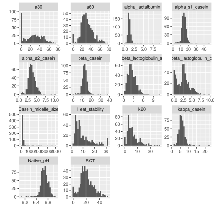
Figure 1: Distributions of the fourteen traits in the regression challenge dataset.

2.1.2 Classification Challenge Dataset.

The dataset comprised 3,275 milk MIR spectra of animals fed one of diet regiments: grass-only (GRS), grass-white clover (CLV) and nutional mix containing grass silage, maize silage, and concentrates (TMR) O’Callaghan et al., (2016); Frizzarin et al., 2021c ; Frizzarin et al., (2023). The task was to predict animal diet type from MIR spectral measurements of the milk samples. The dataset was class balanced with 1,094 spectra for GRS, 1,120 spectra for CLV and 1,061 spectra for TMR. Figure 2 shows the MIR spectra projected to the latent space spanned by the 2 discriminant functions obtained by liner discriminant analysis (LDA). The colouring of the points displays the diet regimen of the animals that the sample had been collected from. The plot illustrates that the spectra from samples from the two pasture classes (GRS and CLV) tend to be similar and are harder to discriminate between, compared to the TMR diet which leads to different milk composition.

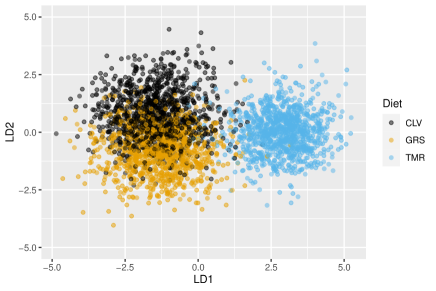
Figure 2: Scatter plot of the MIR spectra from the classification challenge dataset projected on the space spanned by the two latent variables associated with the discriminant functions for milk from cows fed grass (GRS), clover (CLV) and nutional mix (TMR).

2.1.3 MIR Spectra.

The MIR spectra in both datasets were recorded as transmittance values over a sequence of 1,060 wavelengths in the mid-infrared region (regions from 900 cm^-1- 5,000 cm^-1 and 925 cm^-1 - 5,010 cm^-1 for regression and classification respectively). In both datasets, the wavelength transmittance values were transformed to absorbance by taking log₁₀ of the reciprocal of the transmittance value. High-noise-level regions: 1,710 - 1,600 cm^-1, 3,690 -2,990 cm^-1, > 3,822 cm (regression) and 1720 - 1592cm^-1, 3698 - 2996 cm^-1, $>$ 3,818 cm^-1 (classification) were removed from each spectrum. This left 531 and 533 wavelengths respectively for the analyses. Figure 3 shows subsets of the observed mid-infrared milk spectra from the two datasets. The classification challenge spectra are coloured by the diet regimen of the animal from whom the sample was taken.

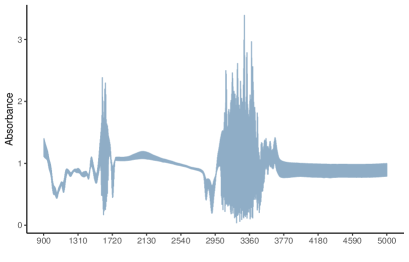
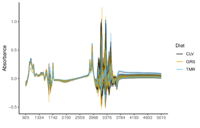
Figure 3: Subsets of the of MIR spectra from the regression challenge dataset (left) and classification challenge dataset (right). In the supervised classification task (right), the colours correspond to the diet regimen of the animal whose sample is plotted.

For the classification task, Fisher score (ratio of between to within diet group variance) and genetic algorithm (GA) Holland, (2019) were used to further reduce the number of input wavelengths. These methods are implemented in R libraries Domijan, (2018) and Willighagen and Ballings, (2022) respectively and the workflow is described in Frizzarin et al., (2023).

The datasets from both challenges involved additional known structure due to sample collection methodology: regression challenge dataset contained samples from different research herds that were collected at evening or morning milking and the classification cohallenge dataset contained samples of repeated measures on same animals collected at different years. As this information was not made available during the competitions, it was not used in the current study to improve prediction models.

2.2 Statistical Analyses

All the analyses were conducted using the R statistical software R Core Team, (2020). The code is available at https://github.com/domijan/ensemblepapercode.

2.2.1 Cross-validation for Regression Challenge.

To compare the performance of different statistical machine learning models, the data were randomly split into 50 training and testing sets. At each random split, candidate models were fit to the training sets. Further ten-fold cross-validation of the training sets was used for algorithm tuning. Test set predictions in each random split were evaluated using root mean squared error (RMSE). The data splitting and model training and evaluating were performed separately for each of the 14 traits.

2.2.2 Cross-validation for Classification Challenge.

Data were randomly split into 10 training and testing sets stratified by diet. The number or random splits was reduced in comparison to the regression challenge to reflect the larger sample size. Candidate models were fit to the training sets with further ten-fold cross-validation for algorithm tuning. As the dataset is class balanced, the predictions for the test sets in each random split were evaluated using accuracy (ACC) which was defined as the proportion of correctly classified samples divided by the total number of samples.

2.2.3 Candidate Models.

The list of candidate models used in the stacking ensembles for the regression and classification challenge is given in Table 1.

Table 1: Candidate Algorithms

Algorithm	Implementation	Challenge
Partial Least Squares (PLS) Garthwaite, (1994)	Mevik et al., (2020)	regression, classification
Linear Regression with PCA (LM + PCA)	base R	regression
Linear Discriminant Analysis (LDA)	Venables and Ripley, (2002)	classification
Least Absolute Shrinkage and Selection Operator (LASSO) Tibshirani, (1996)	Friedman et al., (2010)	regression, classification
Elastic Net (EN) Zou and Hastie, (2005)	Friedman et al., (2010)	regression, classification
Random Forest (RF) Breiman, (2001)	Wright and Ziegler, (2017)	regression, classification
Random Forest with Variable Selection (RF+VS) Wundervald et al., (2020)	Wright and Ziegler, (2017)	regression
Linear Regression with kPCA Schölkopf et al., (1998) (LM + kPCA)	Domijan, (2018)	regression
Random Forest with kPCA (RF + kPCA)	Wright and Ziegler, (2017) , Domijan, (2018)	regression
Random Forest with Gaussian kernel (RF + kernel)	Wright and Ziegler, (2017) , Domijan, (2018)	regression
Support Vector Machine (SVM) Vapnik, (1998)	Karatzoglou et al., (2004)	regression, classification
Bayesian Additive Regression Trees (BART) Chipman et al., (2010)	Kapelner and Bleich, (2016)	regression
Generalized Boosted Regression Model (GBM)Friedman, (2001)	Greenwell et al., (2022)	regression
Bayesian Neural Net (BNN)	Rodriguez and Gianola, (2022)	regression
Neural Net (NNET)	Venables and Ripley, (2002)	classification
Projection Pursuit Regression (PPR) Friedman and Stuetzle, (1981)	base R	regression

Based on their characteristics, the selected candidate models can be grouped into the following classes: dimension reduction methods, regularised regression methods, kernel methods, neural networks and tree based ensemble methods. The classes of models were selected with consideration of their applicability to spectroscopic data and with the aim of increasing the diversity of the models in the library. A very brief outline of each class of methods is given below, with some justification of their choice. A detailed review of these techniques is given in Hastie et al., (2001).

Dimension Reduction Methods.

Spectroscopic data typically comprise a large number of highly serially correlated features. Linear models that involve dimension reduction or variable selection tend to perform well for datasets of this structure. Dimension reduction methods produce a lower dimensional representation of the data using new variables that are derived from linear combinations of the original wavelengths. Partial least squares (PLS) Garthwaite, (1994) for regression and classification is the most well-known and established approach of this type for spectroscopic data. Other approaches tend to combine principal component analysis (PCA) Pearson, (1901) with a linear model such as linear regression in the regression tasks and logistic regression or linear discriminant analysis (LDA) in classification tasks, see for example O’Dwyer et al., (2021). In addition to being a popular algorithm for linear discrimination, LDA also provides a lower dimensional representation of the spectra. Projection pursuit regression (PPR) Friedman and Stuetzle, (1981) is another model that combines dimension reduction with a linear model for prediction.

Regularized Regression Methods.

Regularized regression methods such as Least Absolute Shrinkage and Selection Operator (LASSO)Tibshirani, (1996) and Elastic Net (EN) Zou and Hastie, (2005) include a penalty term in the loss function that has the effect of shrinking some regression coefficients to zero. This leads to variable selection as corresponding wavelengths are removed from the model. The resulting models are more parsimonious and interpretable in contrast with the dimension reduction methods where all the wavelengths are utilised in obtaining the lower dimensional representations of the data. Regularized regression methods can be formulated for the classification tasks using logistic regression. They perform well in highly dimensional datasets with many correlated variables, such as the application in this study, however, the strength of the penalisation is very sensitive to tuning parameters and can strongly affect the fit.

Kernel Methods.

Kernel methods such as Support Vector Machine (SVM) Vapnik, (1998) work well with spectroscopic data as they function through a matrix of pairwise distances of observations across the feature space, rather than the data coordinates. Thus the high dimensionality of the dataset does not increase the complexity of the algorithms and the high correlation does not pose estimation problems. However, if only a small number of wavelengths are useful for the statistical learning task, the additional spurious wavelengths would have the effect of masking the signal in the distance (kernel) matrix, so it can be useful to combine kernel models with a wavelength selection pre-processing step. Different choices of the kernel matrix implicitly map the data to a higher dimensional space where the linear algorithm is applied, therefore elegantly inducing nonlinearity in the models. Model performance can be highly sensitive to the kernel matrix hyper-parameters which require careful tuning.

Neural Networks.

Neural network (NN) models involve constructing new features from linear combinations of the original wavelengths and combining the derived features though a second layer linear regression algorithm. Multiple intermediary layers are constructed, thus producing very flexible, nonlinear models. NNs are particularly successful in domains where the features of the datasets have complicated hierarchical structures such as image or text data. The dataset sizes in this study are not ideal for training deep networks so the architectures were limited to 2-layer networks. Furthermore, deep architectures are complex to tune and computationally burdensome, so are not easily included as candidate models for ensembles.

Tree-based Ensembles.

Tree-based methods fit nonlinear models to the data, but using a different approach from neural networks and kernel based models. A decision tree is a simple model that recursively segments the prediction space into non-overlapping regions. The prediction at each sub-region is the average of the trait measurements (regression) or the most commonly occurring class (classification). Random Forests (RFs)Breiman, (2001) fit multiple trees on bootstrapped samples of the dataset and combine their predictions into a consesus prediction using majority vote (classification) or averaging (regression). Only a subset of randomly selected wavelengths is used for constructing each tree in order to diversify them. Boosting approaches such as Generalized Boosted Regression Model (GBM)Friedman, (2001) fit trees sequentially to the residuals obtained from previously fitted tree. Both are ensemble methods as they borrow strength from a collection of weak-learner algorithms (trees).

2.2.4 Meta-Learners.

To train stacking algorithms, a second layer model (meta-learner) was used to combine predictions from candidate models at each random split. To avoid over-fitting, further ten-fold cross-validation on the training sets within each random split was needed. Meta-learners were trained on the out-of-fold predictions of the candidate models and the resulting coefficients were used to combine predictions in the corresponding test sets from the same random split. Pseudo-code for stacking algorithm implemented for regression challenge is given in Algorithm 1. For the classification challenge, the R based implementation of stacking in package stacks Couch and Kuhn, (2022) was used. The default stacks implementation fits a selection of candidate models over pre-determined grids of tuning parameters and blends the predictions of the candidate models from all the tuning parameter settings in the grids. In contrast, the study presented in this paper used the implementation that combined predictions of tuned models. Note that many variants and implementations of stacking exist. For accessible primers, see, for example, Wolfinger and Tan, (2017) and Naimi and Balzer, (2018).

Standard meta-learner choices are linear regression with a constraint for non-negative coefficients (ens_nonneg) or with shrinkage penalties such as LASSO (ens_LASSO). For the regression challenge we also considered unconstrained linear regression (ens_LM) and a random forest (ens_RF). For the classification challenge we used logistic regression with non-negative restriction for the coefficients (ens_nonneg) which is the default meta-learner in stacks.

For comparison with stacking ensembles and tree based ensemble models, model averaging (regression challenge) and majority vote (classification challenge) were also considered. These ensembles simply combined the test set predictions from the candidate models in each random split. The additional cross-validation layer used for stacking was not needed.

Algorithm 1 Stacking ensemble algorithm pseudo-code

1:Randomly split the dataset into $N$ training and testing sets.

2:for $i\leftarrow 1$ to $N$ do

3:     Use 10-fold cross-validation of training set $i$ to train all candidate models and save their out-of-fold predictions. A further cross-validatory layer may be required for tuning parameters of candidate models.

4:     Combine out-of-fold predictions of candidate models into a dataset and train a meta-learner model.

5:     Train all candidate models on the full training set $i$ and obtain predictions for the corresponding test set $i$.

6:     Use meta-learner coefficients estimated from 4 to combine test set $i$ predictions obtained in 5.

7:end for

2.2.5 Performance Evaluation with the Linear Mixed Model (LME).

Statistical analysis of the data of the prediction performance metrics arising from the study was carried out to compare the predictive ability of different algorithms and the ensemble models. In order to correctly account for the experimental design of our study (algorithms were trained within random splits) when comparing average performance criteria (RMSE, ACC), a linear mixed effects (LME) model Bates et al., (2015) was fit.

Evaluation of the the test set predictions from random splits of the data yielded two new datasets of RMSE or ACC for each of the candidate and ensemble models at each random split. In the regression dataset, RMSE was obtained from modeling the 14 traits which yielded a dataset of 13,300 data points (14 traits $\times$ 50 random splits $\times$ 19 models). In the classification setting, the resulting dataset comprised ACC for 10 random splits $\times$ 9 models, giving 90 data points. To compare the effect of candidate algorithm choice on RMSE or ACC, an LME was fit to the two datasets. In the classification challenge dataset, algorithm type was treated as a fixed effect and in the regression challenge dataset, trait and trait-algorithm interaction were additionally included as fixed effects. The LMEs accounted for within-random split nature of the experimental setting by including random effects for random split id. Post-hoc tests were used to find significant differences between mean RMSE/ACC of different models. R based package effects Fox and Weisberg, (2018) was used to obtain 95% CIs for the effects in Figures 4, 5 and 7.

3 Results

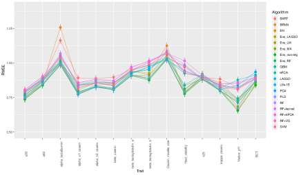
Figure 4: Regression dataset: LME estimates of mean RMSE with 95% CI. Overlapping intervals indicate where the difference is not statistically significant. The interaction plot shows that for most traits (x-axis), the stacking ensemble with non-negative constraint on the coefficients (Ens_nonneg, solid green line), gives lowest mean RMSE.

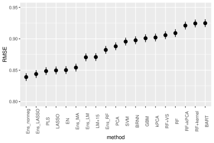
Figure 5: Regression dataset: LME model estimates of mean RMSE over all random splits and traits with 95% CIs. Overlapping intervals indicate where the difference is not statistically significant. The plot shows that the stacking ensemble with the non-negative coefficients gets the lowest average RMSE over all random splits and traits. Second best is stacking ensemble with lasso (Ens_LASSO) and the top candidate algorithms are PLS, LASSO and EN. These candidate models outperform the model averaging ensemble (Ens_MA).

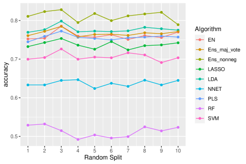
Figure 6: Classification dataset: ACC of algorithms over 10 random splits. Stacking ensemble with non-negative constraint on the coefficients (Ens_nonneg) achieves accuracy of ~81%, which is consistently higher than the best performing candidate model (LDA) with ACC ~78%. Majority vote ensemble gets lower ACC than LDA at all random splits.

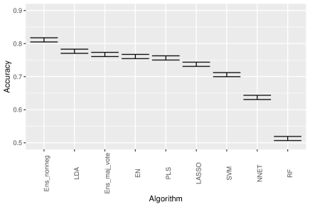
Figure 7: Classification dataset: LME model estimates of mean ACC with 95% CIs by algorithm. The plot shows that the stacking ensemble with the non-negative coefficients gets the highest ACC on average and this is a statistically significant (non-overlapping CIs) improvement on the performance of the best candidate model (LDA). LDA outperforms majority vote ensemble.

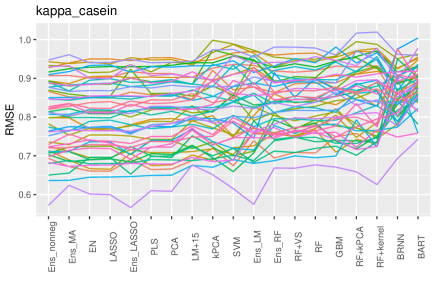
Figure 8: Regression dataset: RMSE of algorithms over 50 random splits for one of the traits $\kappa$-casein.

3.1 Regression Challenge

There is a significant difference in the average RMSE for different algorithms and the significant algorithm-trait interaction (p-value $<$ 0.05) in the regression challenge dataset, indicating some algorithms performed significantly better than others at predicting different traits. This can be seen by non-parallel and intersecting lines in the interaction plot in Figure 4. Non-overlapping 95% CIs for the mean RMSE indicate a significant difference in the prediction performance.

Stacking ensemble with non-negative constraint on the coefficients (Ens_nonneg) consistently performed at least as well as the best candidate model in all traits, which can be seen in Figure 4 where Ens_nonneg achieves lowest average RMSE at all traits.

Figure 5 shows the estimated average RMSE from the LME model. The stacking ensemble with non-negative coefficients gets the lowest average RMSE over all random splits and traits. Second best is stacking ensemble with lasso (Ens_LASSO) and the difference in average RMSE between the two is not statistically significant. These models performed significantly better than other ensemble approaches for blending predictions including linear regression without constraints (Ens_LM) and random forest (Ens_RF). The top candidate algorithms were PLSR, LASSO and EN. These candidate models get lower average RMSE than the model averaging ensemble (Ens_MA).

3.2 Classification Challenge

Figure 6 shows the ACC of all algorithms over 10 random splits in the classification dataset. Stacking ensemble with non-negative constraint on the coefficients (Ens_nonneg) achieves accuracy of ~81%, which is consistently higher than the best performing candidate model (LDA) with ACC ~78%. Majority vote ensemble gets lower ACC than LDA at all random splits.

Figure 7 shows the LME model estimates of mean ACC with 95% CI by algorithm. Overlapping CIs indicate where the difference is not statistically significant. The stacking ensemble with non-negative coefficients (Ens_nonneg) gets the highest ACC on average and this is a statistically significant improvement on the performance of the best candidate model (LDA). LDA outperforms majority vote ensemble model. As in the regression setting, LASSO, EN and PLS outperformed nonlinear models (SVM, RF, NNET).

The regression challenge dataset had a relatively small sample size and in this setting the variability in prediction accuracy due to cross-validatory splits of the data was much larger rather than variability in accuracy of candidate models in all fourteen traits. This is illustrated in Figure 8 which plots RMSE from different algorithms in the test sets from random splits for one of the traits $\kappa$-casein. Plots for other traits (not shown) follow similar pattern. Furthermore, the estimated standard deviation between the random splits in the LME model was twice the estimated residual standard deviation. In the classification challenge dataset which comprised much larger sample size, the LME model estimated the standard deviation between the random splits as half of the estimated residual standard deviation. In this example, the variability in accuracy of different algorithms was larger than the variability in ACC due to random splits, as can be seen in Figure 6.

4 Conclusions

Stacking ensembles with a rich set of candidate models are a versatile tool that researchers can use to improve prediction. The statistical analysis showed that they can consistently improve on the performance of the best candidate models over different datasets and random splits. In the regression dataset, mean RMSE decreased from 0.85 to 0.84, and in the classification dataset mean ACC increased from 0.78 to 0.81. The improvement in performance is modest, however these models have another advantage. Comparative analyses of algorithms in terms of their prediction ability for spectroscopic data have shown that while well established methods like PLS perform strongly, there isn’t a single model that will outperform others in all settings. Results are context specific and can depend on the structure of the dataset at hand Frizzarin et al., 2021b , Singh and Domijan, (2019). Therefore, choosing a single model to generate predictions is unlikely to be the optimal approach, and many potential models are available. Stacking ensembles offer an elegant way of combining predictions of different candidate models.

Since stacking ensemble algorithms use weighted combinations of candidate models to improve performance, the intuition is that increasing the diversity of candidate predictions is likely to increase the chance that ensemble stacking can improve on the predictions of a single strong candidate model. It is worth noting that if the predictions of the candidate models do not show much variation, the aggregation using stacking will add complexity without benefit.

In our stacking ensemble model implementations, candidate models of differing characteristics were selected. LASSO and EN use constrained optimisation to reduce the number of wavelengths that is input into linear models, dimension reduction methods project data to lower dimensional spaces (PLS, LDA, PCA + LM) but retain all wavelengths for computation, regression and classification algorithms that employ different ways of inducing nonlinearity in the model e.g. tree based methods (RF, BART, GBM), kernel based methods (SVM) and neural networks. The tree-based ensemble methods (RF, BART) were the weakest candidate models in terms of their predictive ability for these datasets, whereas linear models like PLS and LDA and regularized regression methods (LASSO, EN) were the strongest candidate models. Spectroscopic data present a specific structure of very high dimension and strong serial correlation between wavelengths, so these classes of models are likely to show a different pattern of performance in different applications.

While there was some variability in algorithm performance for different traits, the LME model showed the stacking ensembles significantly outperformed model averaging (Ens_MA) and majority voting (Ens_maj_vote) ensembles in our application. These are poor approaches to combining model predictions and, on average, performed worse than some candidate models.

Stacking ensemble model implementations can increase diversity of predictions by using different hyper-parameter settings, however we chose to blend the predictions of tuned models. Other ways of enhancing diversity of predictions in the literature involve training the models over different randomly selected subsets of the wavelengths and generating various versions of the training data such as by bagging. This was beyond the scope of the current empirical study. Instead, different choices of meta-learners for blending the predictions were investigated and found that using a non-negative constraint on the coefficients of the linear model gave the best results, which is in agreement with the results of earlier empirical studies Breiman, (1996); Leblanc and Tibshirani, (1996).

References

- Bates et al., (2015) Bates, D., Mächler, M., Bolker, B., and Walker, S. (2015). Fitting linear mixed-effects models using lme4. Journal of Statistical Software, 67(1):1–48.
- Breiman, (1996) Breiman, L. (1996). Stacked regressions. Machine Learning, 24:49–64.
- Breiman, (2001) Breiman, L. (2001). Random forests. Machine Learning, 45(1):5–32.
- Breiman et al., (1984) Breiman, L., Friedman, J., Stone, C., and Olshen, R. (1984). Classification and Regression Trees. Taylor & Francis.
- Chipman et al., (2010) Chipman, H. A., George, E. I., and McCulloch, R. E. (2010). BART: Bayesian additive regression trees. The Annals of Applied Statistics, 4(1):266 – 298.
- Clarke, (2003) Clarke, B. (2003). Comparing bayes model averaging and stacking when model approximation error cannot be ignored. J. Mach. Learn. Res., 4(null):683–712.
- Couch and Kuhn, (2022) Couch, S. and Kuhn, M. (2022). stacks: Tidy Model Stacking. R package version 0.2.3.
- Domijan, (2018) Domijan, K. (2018). BKPC: Bayesian Kernel Projection Classifier. R package version 1.0.1.
- Fox and Weisberg, (2018) Fox, J. and Weisberg, S. (2018). Visualizing fit and lack of fit in complex regression models with predictor effect plots and partial residuals. Journal of Statistical Software, 87(9):1–27.
- Friedman et al., (2010) Friedman, J., Hastie, T., and Tibshirani, R. (2010). Regularization paths for generalized linear models via coordinate descent. Journal of Statistical Software, 33(1):1–22.
- Friedman, (2001) Friedman, J. H. (2001). Greedy function approximation: A gradient boosting machine. The Annals of Statistics, 29(5):1189 – 1232.
- Friedman and Stuetzle, (1981) Friedman, J. H. and Stuetzle, W. (1981). Projection pursuit regression. Journal of the American Statistical Association, 76(376):817–823.
- (13) Frizzarin, M., Bevilacqua, A., Dhariyal, B., Domijan, K., Ferraccioli, F., Hayes, E., Ifrim, G., Konkolewska, A., Nguyen, T. L., Mbaka, U., Ranzato, G., Singh, A., Stefanucci, M., and Casa, A. (2021a). Mid infrared spectroscopy and milk quality traits: A data analysis competition at the international workshop on spectroscopy and chemometrics 2021. Chemometrics and Intelligent Laboratory Systems, 219.
- (14) Frizzarin, M., Gormley, I., Berry, D., Murphy, T., Casa, A., Lynch, A., and McParland, S. (2021b). Predicting cow milk quality traits from routinely available milk spectra using statistical machine learning methods. Journal of Dairy Science, 104(7):7438–7447.
- (15) Frizzarin, M., O’Callaghan, T. F., Murphy, T. B., Hennessy, D., and Casa, A. (2021c). Application of machine-learning methods to milk mid-infrared spectra for discrimination of cow milk from pasture or total mixed ration diets. Journal of Dairy Science, 104(12):12394–12402.
- Frizzarin et al., (2023) Frizzarin, M., Visentin, G., Ferragina, A., Hayes, E., Bevilacqua, A., Dhariyal, B., Domijan, K., Khan, H., Ifrim, G., Nguyen, T. L., Meagher, J., Menchetti, L., Singh, A., Whoriskey, S., Williamson, R., Zappaterra, M., and Casa, A. (2023). Classification of cow diet based on milk mid infrared spectra: A data analysis competition at the “international workshop on spectroscopy and chemometrics 2022”. Chemometrics and Intelligent Laboratory Systems, 234:104755.
- Garthwaite, (1994) Garthwaite, P. H. (1994). An interpretation of partial least squares. Journal of the American Statistical Association, 89(425):122–127.
- Greenwell et al., (2022) Greenwell, B., Boehmke, B., Cunningham, J., and Developers, G. (2022). gbm: Generalized Boosted Regression Models. R package version 2.1.8.1.
- Hastie et al., (2001) Hastie, T., Tibshirani, R., and Friedman, J. (2001). The Elements of Statistical Learning. Springer Series in Statistics. Springer New York Inc., New York, NY, USA.
- Holland, (2019) Holland, J. H. (2019). Adaptation in Natural and Artificial Systems.
- Kapelner and Bleich, (2016) Kapelner, A. and Bleich, J. (2016). bartMachine: Machine learning with Bayesian additive regression trees. Journal of Statistical Software, 70(4):1–40.
- Karatzoglou et al., (2004) Karatzoglou, A., Smola, A., Hornik, K., and Zeileis, A. (2004). kernlab – an S4 package for kernel methods in R. Journal of Statistical Software, 11(9):1–20.
- Laan et al., (2007) Laan, M. J. V. D., Polley, E. C., and Hubbard, A. E. (2007). Super learner. Statistical Applications in Genetics and Molecular Biology, 6.
- Leblanc and Tibshirani, (1996) Leblanc, M. and Tibshirani, R. (1996). Combining estimates in regression and classification. Journal of the American Statistical Association, 91(436):1641–1650.
- McDermott et al., (2016) McDermott, A., Visentin, G., De Marchi, M., Berry, D., Fenelon, M., O’Connor, P., Kenny, O., and McParland, S. (2016). Prediction of individual milk proteins including free amino acids in bovine milk using mid-infrared spectroscopy and their correlations with milk processing characteristics. Journal of Dairy Science, 99(4):3171–3182.
- Mevik et al., (2020) Mevik, B.-H., Wehrens, R., and Liland, K. H. (2020). pls: Partial Least Squares and Principal Component Regression. R package version 2.7-3.
- Moscovich and Rosset, (2022) Moscovich, A. and Rosset, S. (2022). On the Cross-Validation Bias due to Unsupervised Preprocessing. Journal of the Royal Statistical Society Series B: Statistical Methodology, 84(4):1474–1502.
- Naimi and Balzer, (2018) Naimi, A. I. and Balzer, L. B. (2018). Stacked generalization: an introduction to super learning. European journal of epidemiology, 33(5):459–464.
- O’Callaghan et al., (2016) O’Callaghan, T. F., Hennessy, D., McAuliffe, S., Kilcawley, K. N., O’Donovan, M., Dillon, P., Ross, R., and Stanton, C. (2016). Effect of pasture versus indoor feeding systems on raw milk composition and quality over an entire lactation. Journal of Dairy Science, 99(12):9424–9440.
- O’Dwyer et al., (2021) O’Dwyer, K., Domijan, K., Dignam, A., Butler, M., and Hennelly, B. M. (2021). Automated raman micro-spectroscopy of epithelial cell nuclei for high-throughput classification. Cancers, 13(19).
- Pearson, (1901) Pearson, K. (1901). Principal components analysis. The London, Edinburgh, and Dublin Philosophical Magazine and Journal of Science, 6(2):559.
- R Core Team, (2020) R Core Team (2020). R: A Language and Environment for Statistical Computing. R Foundation for Statistical Computing, Vienna, Austria.
- Rodriguez and Gianola, (2022) Rodriguez, P. P. and Gianola, D. (2022). brnn: Bayesian Regularization for Feed-Forward Neural Networks. R package version 0.9.2.
- Schölkopf et al., (1998) Schölkopf, B., Smola, A., and Müller, K.-R. (1998). Nonlinear component analysis as a kernel eigenvalue problem. Neural Computation, 10(5):1299–1319.
- Singh and Domijan, (2019) Singh, M. and Domijan, K. (2019). Comparison of machine learning models in food authentication studies. 30th Irish Signals and Systems Conference, ISSC 2019.
- Stone, (1974) Stone, M. (1974). Cross-Validatory Choice and Assessment of Statistical Predictions. Journal of the Royal Statistical Society. Series B (Methodological), 36(2):111–147.
- Tibshirani, (1996) Tibshirani, R. (1996). Regression shrinkage and selection via the lasso. Journal of the Royal Statistical Society: Series B (Methodological), 58:267–288.
- Vapnik, (1998) Vapnik, V. (1998). Statistical Learning Theory. Wiley-Interscience, New York.
- Venables and Ripley, (2002) Venables, W. N. and Ripley, B. D. (2002). Modern Applied Statistics with S. Springer, New York, fourth edition. ISBN 0-387-95457-0.
- Visentin et al., (2016) Visentin, G., Penasa, M., Gottardo, P., Cassandro, M., and De Marchi, M. (2016). Predictive ability of mid-infrared spectroscopy for major mineral composition and coagulation traits of bovine milk by using the uninformative variable selection algorithm. Journal of Dairy Science, 99(10):8137–8145.
- Willighagen and Ballings, (2022) Willighagen, E. and Ballings, M. (2022). genalg: R Based Genetic Algorithm. R package version 0.2.1.
- Wolfinger and Tan, (2017) Wolfinger, R. D. and Tan, P.-Y. (2017). Sas-2017 stacked ensemble models for improved prediction accuracy.
- Wolpert, (1992) Wolpert, D. H. (1992). Stacked generalization. Neural Networks, 5(2):241–259.
- Wright and Ziegler, (2017) Wright, M. N. and Ziegler, A. (2017). ranger: A fast implementation of random forests for high dimensional data in C++ and R. Journal of Statistical Software, 77(1):1–17.
- Wundervald et al., (2020) Wundervald, B. D., Parnell, A. C., and Domijan, K. (2020). Generalizing gain penalization for feature selection in tree-based models. IEEE Access, 8:190231–190239.
- Zou and Hastie, (2005) Zou, H. and Hastie, T. (2005). Regularization and variable selection via the elastic net. Journal of the Royal Statistical Society. Series B: Statistical Methodology, 67:301–320.