Remote sensing framework for geological mapping via stacked autoencoders and clustering

Abstract

Supervised learning methods for geological mapping via remote sensing face limitations due to the scarcity of accurately labelled training data. In contrast, unsupervised learning methods, such as dimensionality reduction and clustering, have the ability to uncover patterns and structures in remote sensing data without relying on predefined labels. Dimensionality reduction methods have the potential to play a crucial role in improving the accuracy of geological maps. Although conventional dimensionality reduction methods may struggle with nonlinear data, unsupervised deep learning models such as autoencoders have the ability to model nonlinear relationship in data. Stacked autoencoders feature multiple interconnected layers to capture hierarchical data representations that can be useful for remote sensing data. In this study, we present an unsupervised machine learning framework for processing remote sensing data by utilizing stacked autoencoders for dimensionality reduction and k-means clustering for mapping geological units. We use the Landsat-8, ASTER, and Sentinel-2 datasets of the Mutawintji region in Western New South Wales, Australia to evaluate the framework for geological mapping. We also provide a comparison of stacked autoencoders with principal component analysis and canonical autoencoders. Our results reveal that the framework produces accurate and interpretable geological maps, efficiently discriminating rock units. We find that the stacked autoencoders provide better accuracy when compared to the counterparts. We also find that the generated maps align with prior geological knowledge of the study area while providing novel insights into geological structures.

[1]Machine Learning Lab, International Institute of Information Technology, Hyderabad, India [2]EarthByte Group, School of Geosciences, The University of Sydney, Sydney, Australia [3]School of Earth and Planetary Sciences, Curtin University, Perth, Australia [4]Transitional Artificial Intelligence Research Group, School of Mathematics and Statistics, University of New South Wales, Sydney, Australia

1 Introduction

Geological mapping is useful for different purposes, e.g., studying the mineralisation potential of a region and creating prospectivity maps [1, 2, 3]. Remote sensing provides an alternative to traditional fieldwork for geological mapping, which is costly in terms of time and resources and sometimes infeasible due to different circumstances such as harsh topography or political reasons [4]. Optical remote sensing images acquired by the scanners mounted on different platforms, such as satellites, include multiple spectral bands ranging from visible to infrared portion of the electromagnetic spectrum [5]. Radiance is measured by multispectral scanners in visible and near-infrared (VNIR, 400-1000 nm) and short-wavelength infrared (SWIR, 1000-2500 nm). The amount of information contained in multispectral images can aid in geological analysis, particularly for identifying and mapping the distribution of rocks and minerals due to their specific spectral absorption properties [6, 7, 8]. This is the basis of spectrum-based approaches for classifying and mapping pixels of an image. The spectral and spatial resolution provided by remote sensing data, particularly those acquired by satellites, makes identifying rock units in vast areas feasible [9]. On the other hand, geological mapping based on remote sensing is challenging given the complexities involving sub-pixel level noise and inconsistencies [10], mixing of minerals, thick layers of regolith [3], and lack of data due to vegetation and cloud cover [11]. To address these challenges, a number of studies have been carried out, and different frameworks proposed [12, 13, 14].

Common geological mapping techniques involve comparing absorption features to reference spectra or training samples [6]. However, it is challenging to collect a sufficient number of pixels as reference spectra or training samples. Geological processes determine spectral variability in rocks based on their chemical and mineral composition, grain size, texture, and structure. [15]. Spectral variability of rocks in a study area significantly affects geological mapping using remote sensing data. As such, an insufficient number of training samples with highly correlated spectral bands often leads to a number of problems when discriminating rock units [16]. Therefore, it is necessary to extract useful information in images and remove redundant information to improve geological discrimination [17].

Machine Learning models have proven to be powerful tools for extracting valuable information from multi-spectral images and mapping geochemical anomalies [18]. These techniques leverage dimensionality reduction, clustering, and classification approaches to automatically analyze and interpret complex data sets [19, 20, 21, 22]. In the case of remote sensing, machine learning models found widespread applications [23], and their adoption in mineral exploration has been gaining significant traction [3]. Unsupervised machine learning techniques such as dimensionality reduction and transformation methods, have demonstrated remarkable efficiency in discriminating between geological units, which makes them invaluable for identifying and mapping geochemical anomalies [24]. Transformation techniques such as principal component analysis (PCA) [25], independent component analysis (ICA) [26, 27], and minimum noise fraction (MNF) [28] have been used for suppressing irradiance that dominates all bands of remote sensing data [29], thereby, enhancing the spectral reflectance of geological features [30]. In contrast, supervised learning techniques (trained with labels in data) can partially resolve the issues with semi-manual analysis by automating feature extraction, which requires ground truth data and expert input that are costly and mainly depend on the interpretation that can be biased [31]. A limited collection of fully labelled and high-quality training images for geological features is publicly available to compound the challenge of the supervised learning techniques above. Furthermore, supervised learning techniques can be applied to multivariate datasets, such as multispectral remote sensing data, to extract specific spectral responses from different rock units [32, 33], but large spectral variability and limited training data availability make classification a difficult task for geological analysis of remotely sensed data.

Autoencoders [34] are a class of artificial neural networks primarily used for unsupervised learning tasks, such as dimensionality reduction and feature learning [35, 36]. They are composed of two major components which include an encoder and a decoder. Autoencoders are based on the concept of change variable method [37, 36], helping to make data easier to understand by breaking it down into simpler parts (low dimensions). They can be used to represent the data with much fewer features assuming that the input dataset has low-dimensional latent representation. The latent vector of autoencoders represents the reduced feature dimension, which is used in remote sensing data processing to extract features or structures such as geological units [38]. Features in the reduced representation obtained by autoencoders correspond to different types of minerals [39, 40], and as such, enforcing feature independence would prevent mixed minerals from being identified. Recently, [38] proposed to handle noise in the input signals, attributed to dimensionality redundancy, and without sacrificing important features. Stacking is an ensemble learning approach [41] that can further improve autoencoders. Stacked autoencoders have been useful in several other applications, such as feature extraction for multi-class change detection in hyperspectral images [42], and classification of multispectral and hyperspectral images [43, 44]. Stacked autoencoders provide a powerful framework for learning deep representations of data in an unsupervised manner, which can be beneficial for various machine learning tasks, particularly when labeled data is scarce or expensive to obtain. Stacking autoencoders also has the potential to aid in learning the nonlinearity between spectral bands and discriminating between complex features such as geological units.

The output components or extracted latent vectors of dimensionality reduction or transformation techniques can be used as input for the clustering methods, such as the k-means algorithm to cluster pixels and map geological units [45, 40]. Clustering methods are unsupervised learning methods [45, 46] that organise a dataset into different groups based on the similarity of samples (instances) using some distance measures [47, 48]. Clustering methods have been prominently used in remote sensing applications in conjunction with dimensionality reduction methods [49], e.g., for pixel clustering [50], fuzzy clustering for change detection [51], image segmentation [52], mean-shift clustering of multispectral imagery [53], and hyperspectral image subspace clustering involving dimension reduction, subspace identification, and clustering [54]. However, clustering methods suffer from the curse of dimensionality, rendering their usage in remote sensing data processing challenging. In large datasets, such as multispectral remote sensing applications, the power of autoencoders and clustering can be jointly harnessed to address the limitations and challenges of conventional methods. In remote sensing-based geological mapping, a major challenge arises from the intricate and diverse nature of geological features coupled with the often remote and inaccessible locations of geological sites.

In this study, we present an unsupervised framework that combines stacked autoencoders for dimensionality reduction and k-means clustering to map geological units for mineral prospecting. The role of the stacked autoencoders is to compress the data that has a wide range of spectral and spatial features. We use k-means clustering to generate clustered maps from the reduced dimensions in the framework. We evaluate the framework across multiple datasets, including Landsat 8, ASTER, and Sentinel-2 multispectral datasets to map geological units in the Mutawintji region, Western New South Wales (NSW), Australia. We compare the results against PCA and canonical autoencoders as a benchmark study.

2 Materials and Methods

2.1 Geological setting

The Mutawintji region is located in the far west of NSW and the semi-arid zone of the state. It is approximately 1,150 km west of Sydney and covers an area of approximately 700 $km^{2}$ within the Curnamona Province, a geological province that covers a large area of southeastern Australia. As shown in Figure 1a, the study area is situated on the eastern margin of the Curnamona Province, characterised by a thick sequence of sedimentary rocks deposited in a shallow marine environment during the Cambrian and Ordovician periods [55]. The geological setting of the study area is dominated by sedimentary rocks of the Cambrian and Ordovician periods, which are around 500 to 480 million years old. However, Quaternary residual and colluvial deposits cover a significant part of the sedimentary rocks [56]. The sedimentary rocks comprise various rock types, including sandstone, shale, siltstone, and limestone. These rocks were formed by the accumulation of sediments in an ancient sea that covered much of the region during the Cambrian and Ordovician periods. The sediment was later buried and compressed, eventually forming the sedimentary rocks that can be observed on the surface. In addition to the sedimentary rocks, the geology of the study area also includes a range of other rock types, including volcanic rocks and granites. Major faults in the study area strike N–S or NW–SE, which separate Ordovician quartzite and sandstone units from shale, siltstone, and limestone in the southwest. Overall, the geology of the study area, as shown in Figure 1b, is characterised by a complex and diverse range of rock types that reflect the region’s long and varied geological history and make it an interesting area for our study.

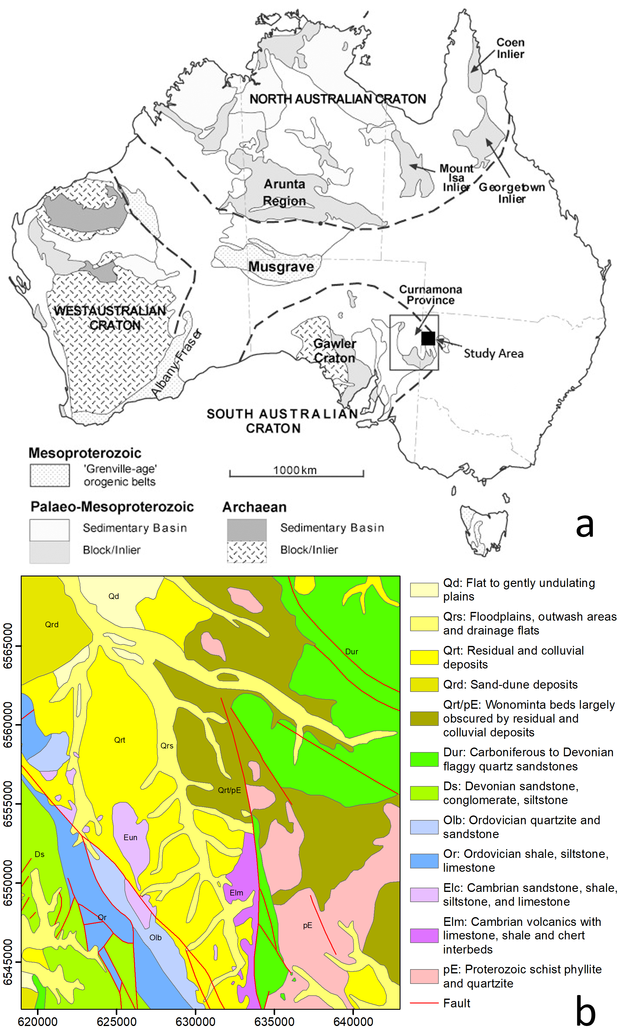
Figure 1: a) The Curnamona Province and other Proterozoic terrains in Australia [57]; the study area has been shown using a black square. b) Simplified geological map of the study area.

2.2 Remote sensing data and pre-processing

The proposed framework is implemented on three different types of multispectral remote sensing data, Landsat 8, ASTER, and Sentinel-2, to map geological units. The detailed technical performance and attributes of these data types can be found in [3]. Landsat 8, launched in 2013, carries two sensors - the Operational Land Imager (OLI) and the Thermal Infrared Sensor (TIRS). The satellite provides images in 11 different spectral bands. The resolution of these bands ranges from 15 meters (m) for the panchromatic band to 30 m for the VNIR and SWIR bands. The last two bands, which are thermal bands numbered 10 and 11, have a resolution of 100 m [58]. Geological remote sensing for mapping purposes significantly improved with the launch of the ASTER sensor on the Terra platform in 1999. The ASTER VNIR bands have a spatial resolution of 15 m, followed by six SWIR bands with 30 m resolution and five thermal infrared bands with 90 m resolution [59]. The Sentinel-2A and Sentinel-2B are twin satellites in a sun-synchronous orbit phased 180 degrees apart. The onboard multispectral instrument captures data in 13 spectral bands ranging from VNIR to SWIR. The Sentinel-2 images have varying spatial resolutions ranging from 10 to 60 m [60]. In this study, we use spectral bands of greater importance in geological remote sensing due to their characteristic behaviours, such as high absorption or reflectance in different geological units, allowing us to generate meaningful geological maps. Accordingly, seven bands of OLI (bands 1–7), nine bands of ASTER (bands 1–9), and ten bands of Sentinel-2 (bands 2–8, 8a, 11, and 12) are selected as input to the framework [3].

A cloud-free Landsat 8 scene of the study area was obtained from the US Geological Survey Earth Resources Observation and Science (EROS) centre . The image captured on 5 October 2021 is a level-1T image that has been terrain-corrected. The ASTER image utilised in this study was acquired on 10 August 2001, a cloud-free level-1-precision terrain-corrected registered at-sensor radiance product (ASTER_L1T) obtained from the USGS EROS centre. A cloud-free Sentinel-2A scene of the study area captured on 19 March 2022 was also acquired from the European Space Agency via the Copernicus Open Access Hub via scihub.copernicus.eu (accessed on 28 March 2022). The Sentinel-2 image used in this study is a level-1C product that has undergone radiometric and geometric corrections, as well as orthorectification, resulting in top-of-atmosphere reflectance values.

The remote sensing datasets used in this study are pre-georeferenced to the universal transverse Mercator (UTM) zone 54 South, and no geometric correction is needed. The Landsat 8 OLI and ASTER data are radiometrically corrected, and the reflectance data are used as input. The SWIR bands in the ASTER data are resampled using the nearest neighbour technique to match the spatial resolution of the VNIR bands, which is 15 m. After resampling, a data layer is created by stacking the VNIR and SWIR bands for further processing. The Sentinel-2 image used in this study includes the atmospheric correction. The Sentinel-2 VNIR and SWIR bands are stacked using the nearest neighbour technique to create a 10-band dataset with 10 m spatial resolution. Before processing the datasets, all images are adjusted to meet the target area size by resizing them.

2.3 Stacked autoencoders

The autoencoder is a dimensionality reduction technique used to uncover a lower-dimensional manifold, also known as the latent space of intrinsic dimensionality, while preserving the essential information present in the original data. The stacked autoencoder architecture comprises of multiple layers of autoencoders, where each layer is trained independently as an individual autoencoder [61]. The output from the previous layer is used as input for the subsequent layer, allowing the network to learn hierarchical representations of the data. A typical stacking approach will have at least two layers, where the first layer features several models (can be any machine learning model) and the second layer combines the predictions (output) using a simpler model that is also trained. The first layer enables to capture meaningful features and patterns in the case of a multi-spectral image dataset as shown in Figure 2. Additionally, Stacked architecture acts as a regularizer, preventing overfitting by forcing the model to learn more generalized features because each layer acts as a feature extractor, reducing the dimensionality of the data and forcing the model to learn more generalisable features. Stacked autoencoders can be used to extract features from the input data for use in other machine learning models to improve their performance [62].

Figure 3a depicts a canonical autoencoder consisting of an encoder that reduces the dimensionality of the input data and a decoder that generates the original data from the encoded representation. Autoencoders can learn more abstract and higher-level features of the data, while PCA only finds linear combinations of the original features. This can be useful when data has complex patterns and structures. PCA is a simple and easy-to-understand method for dimensionality reduction, while autoencoders can be more complex and require more training time and computational resources [44]. PCA can generalise well to new, unseen data, while autoencoders may overfit the training data and perform poorly on new data if not properly regularised [63].

Unlike linear dimensionality reduction methods, such as PCA, autoencoders do not strive to keep a specific attribute, such as distance or topology. Sometimes, the connection between the input characteristics is deep and nonlinear [64], and typical dimensionality reduction methods fail to produce good results [65]. The staked autoencoder has been designed because the canonical autoencoder is insufficient to handle the nonlinearity problem in many applications [66]. Multiple autoencoders are layered above one another to form stacked autoencoders. Figure 3b depicts a layered autoencoder with three encoders and decoders stacked on top of one another [67]. The architecture of a stacked autoencoder is all learned from the data, ensuring that the learned model reflects data characteristics and avoids choosing the nonlinear function manually. It is challenging to identify whether the relationship between spectral bands of a remote sensing dataset and target characteristics is linear or nonlinear. The stacked autoencoder is employed to take care of both global and local characteristics in the dataset and reduce the dimensionality of the datasets.

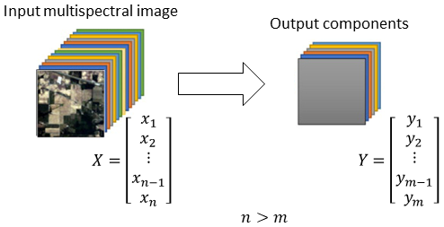
Figure 2: The visualisation of the dimensionality reduction for a multispectral dataset. The number of input spectral bands $n$ is reduced to $m$ in the output dataset. Each coloured layer in the input image and the output represents a spectral band and a component, respectively.

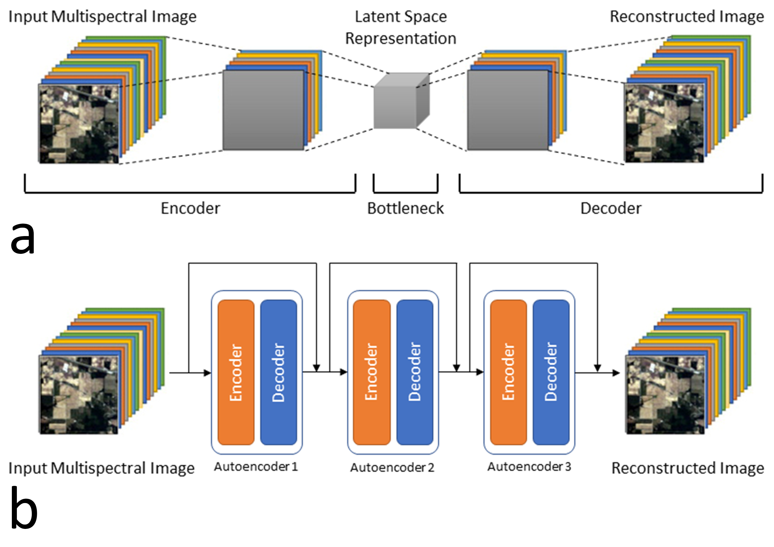
Figure 3: a) Architecture of a canonical autoencoder consisting of an encoder and a decoder. The encoder takes the multispectral image as input ($x$) and reduces the dimension to the latent vector ($z$), where dim($x$) $>=$ dim($z$). The decoder reconstructs the image from the latent vector ($Z$). b) A stacked autoencoder with three encoders and decoders for each stacking level. The encoder and decoder architecture in each stack level is the same as the canonical autoencoder, with two hidden layers for each.

2.4 K-means clustering

Clustering algorithms are unsupervised machine learning methods that divide a dataset into a specific number of groups (clusters) based on a distance measure of the data instances. There are different types of clustering methods, such as k-means, fuzzy c-means, mountain clustering, and subtractive clustering [68, 47, 48, 22]. k-means clustering is a simple, efficient, and computationally fast algorithm for image segmentation [68]. The k-means algorithm determines $k$ cluster centres given $k$ seed centres. The k-means algorithm assigns each pixel in the image to the cluster whose centre is closest to the pixel. Next, it calculates new cluster centres by averaging all pixels in a group and repeats for a particular number of iterations.

The optimal number of clusters in k-means is a user-defined hyperparameter, and several methods exist to determine the optimal number of clusters [69]. The elbow method is a popular and heuristic technique to validate or find the optimal number of clusters [70]. This method uses the idea of the within-cluster sum of squares (WCSS) value, which defines the total number of variations within a cluster. As the number of clusters increases, the WCSS will decrease as the points become more closely aligned with their closest cluster centre. The elbow method takes advantage of this trend by plotting the WCSS against the number of clusters and selecting the number of clusters where the WCSS starts to level off, typically indicated by a noticeable elbow in the plot [70]. The Elbow method involves plotting the inertia($k$) against the number of clusters $k$. The optimal number of clusters is chosen at the point where the curve starts to flatten, forming an ”elbow” shape. This point represents the trade-off between minimizing the inertia and keeping the number of clusters small and aims to find the value of $k$.

The k-means algorithm assigns all members to $k$ clusters, even if $k$ is not optimal for the dataset, but the elbow method involves running k-means clustering on a dataset using different values of $k$ and computing an average score for each value of $k$. As the number of clusters increases, the WCSS value will start to decrease, and the cluster number, after which the graph turns into a flat line, is considered the optimal $k$ or the number of clusters for some $\alpha$ greater than zero.

2.5 Framework

The successful implementation of deep learning algorithms in geological mapping necessitates a multidisciplinary approach integrating specialised domain-specific knowledge and tailored neural network architectures. Autoencoders can be more robust to outliers and noisy data than PCA, as they can learn to ignore or suppress noisy features during training [71]. In this study, we leverage stacked autoencoders pre-train weights (trained on a large dataset) and fine-tune the weights with training model on the three datasets to enhance their effectiveness in accurately identifying geological features. As shown in Figure 4, the first step is acquiring multispectral images (Landsat 8, ASTER, and Sentinel-2), followed by required radiometric and geometric corrections and data scaling that constitute the pre-processing stage. The next two stages include dimensionality reduction and categorisation of pixels using the learnt features from the data with reduced dimensions. Each pixel is regarded as a collection of non-spatial spectral observations by spectral classifiers. The pre-processed data are imported into the dimensionality reduction methods, i.e., PCA, canonical autoencoders, and stacked autoencoders. We determine the optimal number of clusters using the Elbow method and use the output components of the dimensionality reduction methods and the k-means clustering method to provide the clustered maps that represent geological maps. Moreover, to compare different dimensionality reduction methods and data types, we use the Davies-Bouldin index, sometimes referred to as the variance ratio criteria, and the Calinski-Harabasz index, which can be calculated without labelled data [69]. The Calinski-Harabasz criterion has a big index for between-cluster variation and a small index for within-cluster variance. Therefore, the ideal number of clusters corresponds to the maps with a high Calinski-Harabasz index, in contrast to the Davies-Bouldin index.

As detailed in [72], our findings indicate that neighboring pixels in images tend to have high likelihoods of belonging to the same cluster due to spatial correlation, a property that aids in the clustering process. Geological units typically have regional distributions in space [73], meaning that adjacent pixels of similar properties are likely to belong to the same geological unit. Each group of pixels may be close to a neighbouring cluster and may create confusion. In geology, the majority of filters can be applied to geological data to improve the accuracy and consistency of the map by removing outliers and inconsistencies along with the noise associated with the data. The majority of filters can help generate more accurate and reliable geological maps, which can provide a better understanding of the geology of an area. In this study, we apply the majority filter with the kernel size of $7\times 7$ to the maps, changing spurious pixels within a large single class to that class. The centre pixel in the kernel is replaced with the class value that a majority of the pixels in the kernel have [74].

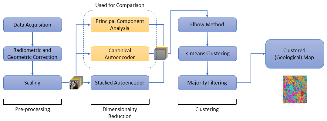
Figure 4: Proposed framework for creating geological maps using the integration of the dimensionality reduction (PCA, canonical autoencoder, and stacked autoencoder) methods and the k-means clustering algorithm.

2.6 Experimental setup

We implement the framework in Figure 4 using the Python programming language and various libraries, including Keras. These tools allow for the efficient implementation and execution of the deep learning models used in the study and facilitate the development and testing of the models, allowing for a streamlined and efficient experimentation process. Implementing each machine learning models requires setting a number of hyperparameters. This study experiments with different values to create each model and selects those providing the most accurate result. In the case of PCA, the components preserving 90 percent of the total variance of the input spectral bands are kept, resulting in a different number of components for each data type. In the architecture of the canonical autoencoders, we use five hidden layers and ten iterations (epochs). Moreover, we use the scaled exponential linear unit (SELU) [75] as the activation function for the hidden layers and the sigmoid activation for the output layer. We use the Adam optimiser [76] and mean squared error (MSE) loss function for training with an initial learning rate of 0.01. The architecture of the stacked autoencoders used in this study is more complicated than the canonical autoencoders. Each of the stacked autoencoders includes three canonical autoencoders. The first two autoencoders have five hidden layers, but the last autoencoder has seven hidden layers. The optimiser and the loss and activation functions for the hidden and output layers are the same as the canonical autoencoders. We implement the experiments in a Keras Python framework using 11th Gen Intel(R) Core(TM) i7-11700 @ 2.50GHz CPU.

3 Results

We apply our proposed framework on the Landsat 8, ASTER, and Sentinel-2 images of the Mutawintji region in western New South Wales, Australia. Figure 5 shows the elbow graphs applied to determine the optimal number of clusters for different pairs of data types and dimensionality reduction methods. In these plots, the optimal $k$ for the k-means clustering has been shown using a green dashed line, and the black line shows the sum of squared distances of the centre of clusters. In elbow plots, the point at which the maximum curvature occurs indicates the optimal $k$, using which the model fits [77]. The optimal numbers of clusters are also summarised in Table 1, where the majority is six, implying that there are six major geological units in the study area, that show specific spectral characteristics detected by the multispectral datasets.

In addition to PCA, we train the canonical and stacked autoencoders and calculate the reconstruction loss, which showcases that the loss of information/features after dimensionality reduction is low. The learned features from canonical and stacked autoencoders are used to cluster remote sensing data. It is observed that the loss comes into the saturation state after a few epochs. Different metrics are available to quantitatively evaluate the efficiency of a clustering process without the need for labelled data, such as the Silhouette Coefficient, Calinski-Harabasz, and Davies-Bouldin scores [69]. Due to the high number of pixels, calculating the Silhouette Coefficient takes a long time on a personal computer and is not a practical solution. Therefore, we evaluate the performance of the models using the Calinski-Harabasz and Davies-Bouldin scores [78, 40] as shown in Table 2. A lower Calinski-Harabasz score (first column for each method in Table 2) correlates with better-defined clusters, while the higher Davies-Bouldin score (second column for each method in Table 2) shows a more efficient clustering result.

Figure 6 shows the clustered or geological maps obtained by applying the proposed framework to different pairs of remote sensing data and dimensionality reduction methods. The geological maps created using PCA followed by k-means show different characteristics than those generated by canonical and stacked autoencoders. The maps generated by employing stacked autoencoders on Landsat 8 and ASTER, along with canonical autoencoders and Sentinel-2, involve seven clusters, and the rest have six clusters. In addition to the metrics mentioned above, we use 30 rock samples and the information associated with them provided by the Geological Survey of NSW as ground-truth data. We calculate the overall accuracy of each pair of the dimensionality reduction methods and remote sensing data by dividing the correctly clustered samples by the total number of samples (Table 3). Since the calculated optimal number of clusters for all the pairs of data types and dimensionality reduction methods are not the same, we simplify the rock types of the samples and categorise them into six (Figure 7a) or seven classes according to Table 1.

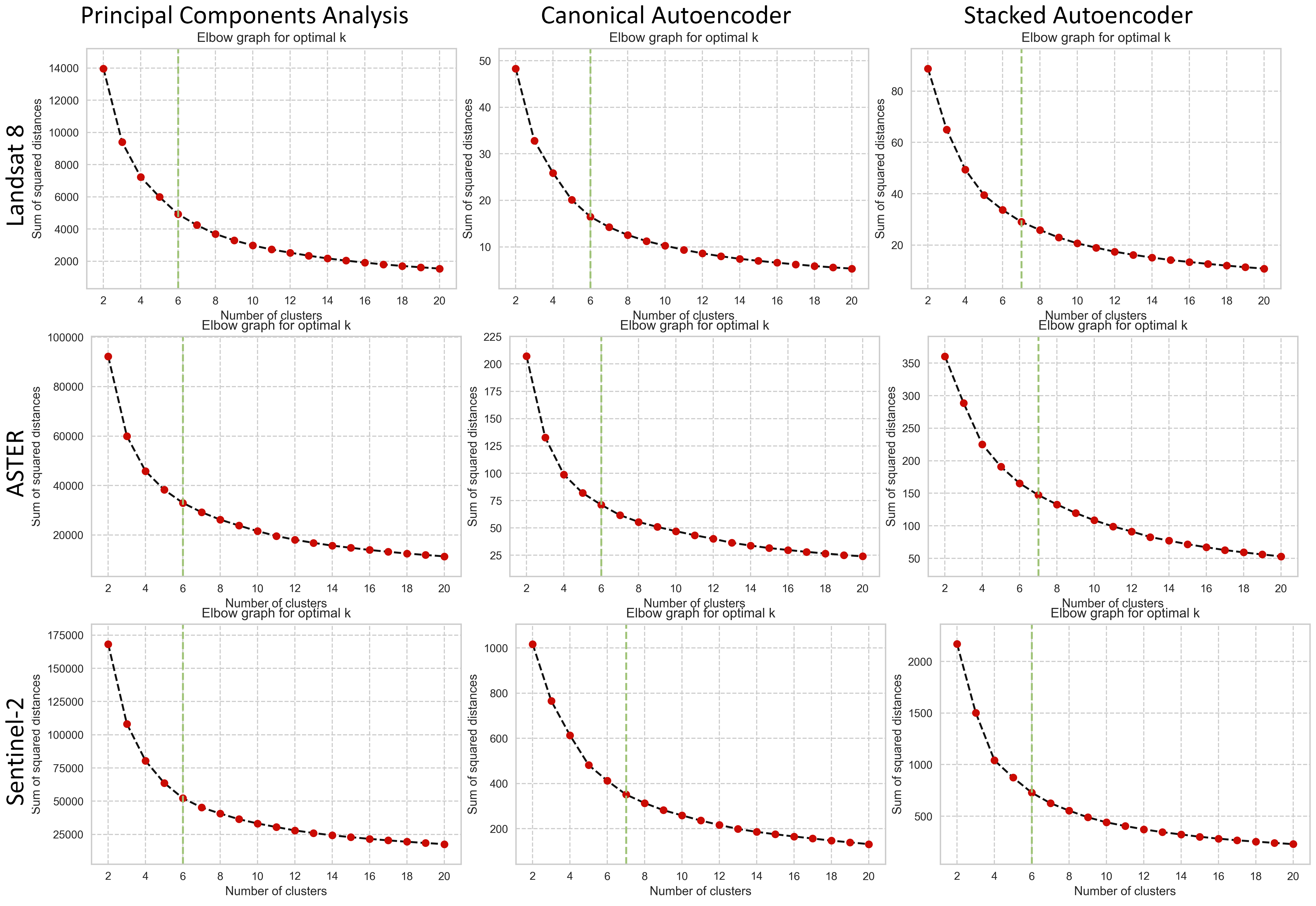
Figure 5: Elbow plots obtained for each pair of the data types and dimensionality reduction methods. The green dashed lines represent the optimal number of clusters.

Data Type/Method	PCA	Canonical Autoencoder	Stacked Autoencoder
Landsat 8	6	6	7
ASTER	6	6	7
Sentinel 2	6	7	6

Table 1: Optimal number of clusters determined for the k-means clustering algorithm using different pairs of data types and dimensionality reduction methods.

Data Type	PCA		Canonical Autoencoder		Stacked Autoencoder
	Calinski-Harabasz	Davies-Bouldin	Calinski-Harabasz	Davies-Bouldin	Calinski-Harabasz	Davies-Bouldin
Landsat 8	725156	0.848	712419	0.803	560856	0.826
ASTER	3203478	0.882	3127690	0.897	1645733	0.907
Sentinel 2	7975444	0.799	4672222	0.829	5018638	0.860

Table 2: Calinski-Harabasz (CH) and Davies-Bouldin (BD) scores calculated between clusters for different pairs of data types and used dimensionality reduction methods. Blue color: best results.

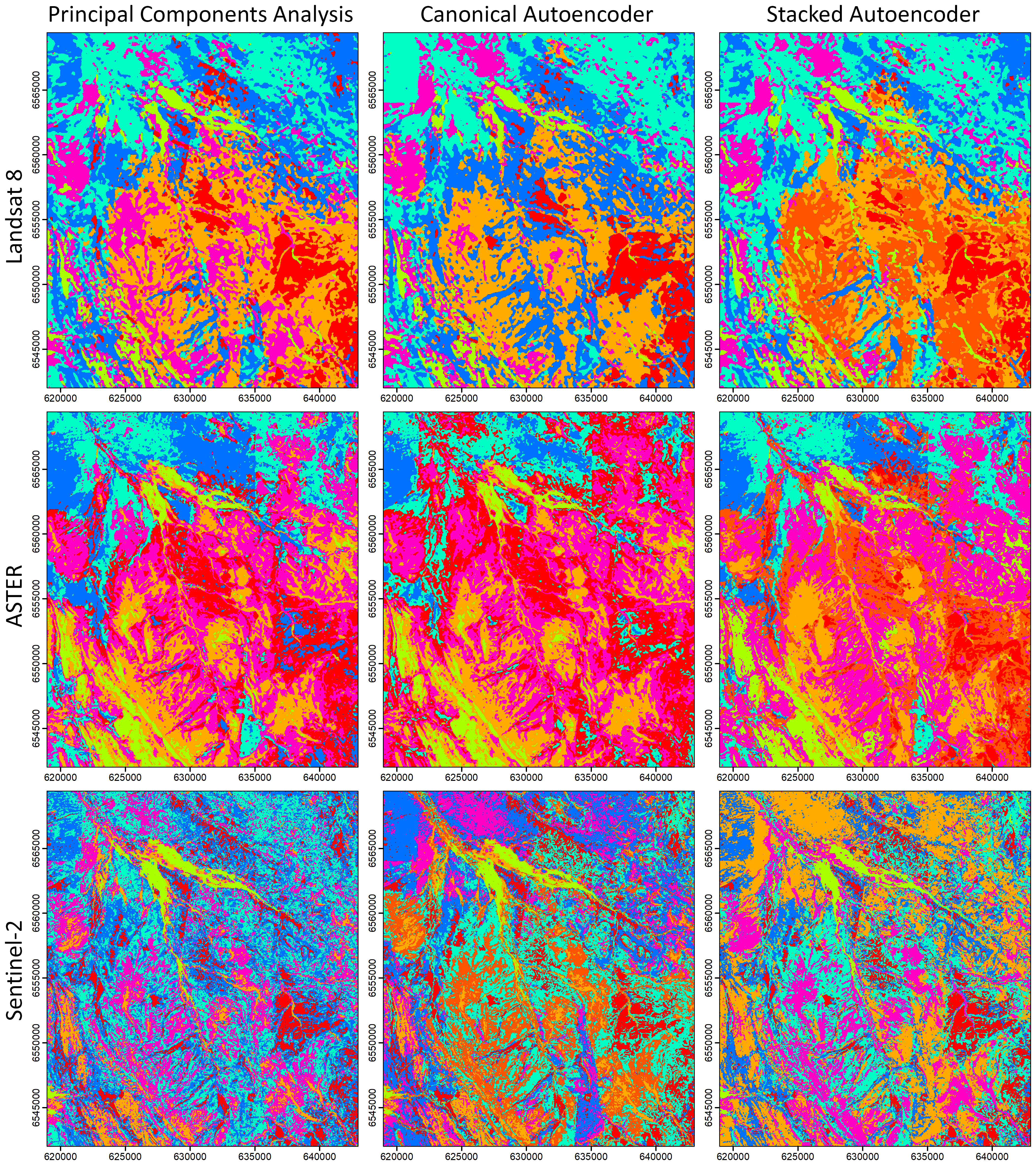
Figure 6: Clustered maps of the study area obtained by different pairs of data types and dimensionality reduction methods. Each coloured area in the maps represents a unique geological unit on the ground.

Data Type/Method	PCA	Canonical Autoencoder	Stacked Autoencoder
Landsat 8	0.760	0.733	0.767
ASTER	0.800	0.800	0.833
Sentinel 2	0.800	0.833	0.900

Table 3: Overall accuracy of different pairs of data types and dimensionality reduction methods. Blue color: best accuracy.

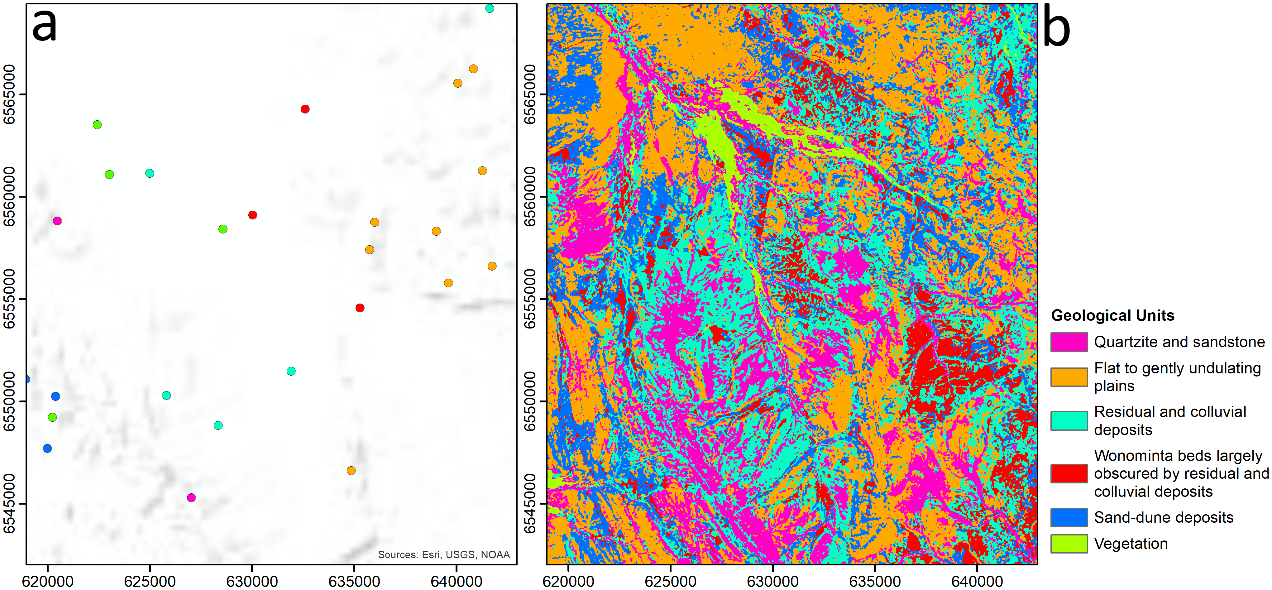
Figure 7: a) Rock samples collected in the study area; b) Interpreted clustered map obtained by implementing the proposed framework and applying stacked autoencoders to the Sentinel-2 dataset.

The maps are primarily compared regarding the efficiency of different dimensionality reduction methods for removing noise, compressing data, and discriminating between geological units. Autoencoders are non-linear models that can capture complex relationships in the data. Conversely, PCA is a linear model that can only capture linear relationships between variables. Three different metrics are calculated to validate the proposed framework and compare different dimensionality reduction methods quantitatively. According to Table 2, PCA results in larger Calinski-Harabasz scores for each data type, which indicates that the centre of clusters generated using the PCA output components and the k-means algorithm are more separable compared to autoencoders because PCA does not consider the feature dependency. It is also observed that as the spatial resolution increases, the Calinski-Harabasz score improves, and Sentinel-2 results in higher scores due to higher spatial resolution. Among all the data types and dimensionality reduction methods, the use of PCA on Sentinel-2 results in the highest Calinski-Harabasz score.

The investigation of Davies-Bouldin scores in Table 2 reveals that the average values of this metric for PCA and canonical autoencoders are the same, and the average is slightly higher for stacked autoencoders. According to Table 2, using PCA on Sentinel-2 data results in the lowest score, which is interpreted as the best result. In contrast to Calinski-Harabasz scores, a higher spatial resolution does not necessarily improve the Davies-Bouldin score. ASTER data shows the highest score for each method, which means this data type is not preferred for discriminating between geological units compared to other data types. Moreover, Sentinel-2 and Landsat 8 show a similar average score.

Each coloured area in the maps shown in Figure 6 represents a unique geological unit clustered by the k-means algorithm and a pair of data types and dimensionality reduction methods. By comparing the clustered maps with the geological map shown in Figure 1b, it is obvious that Sentinel-2 data provides a more detailed clustered map than other data types and conventional approaches for mapping geological units. This data type is the only one that detects vegetation correctly and assigns a separate cluster to the relevant pixels. The comparison of the dimensionality reduction methods also shows that only stacked autoencoders are able to more accurately discriminate between different sedimentary units in the south and southeast of the study area. Using high-resolution remote sensing data like Sentinel-2 and benefiting from the power of non-linear dimensionality reduction methods like stacked autoencoders to increase the signal-to-noise ratio of the input features to the clustering algorithms results in more detailed and accurate geological maps than conventional approaches.

The metrics reported in Table 2 and discussed above do not consider the ground truth or labelled data and merely rely on the input features and the labels assigned to each observation or pixel. The overall accuracy presented in Table 3 considers the adaptation of collected rock samples from the study area shown in Figure 7a with the clustered maps, a more reliable metric for determining the best approach for generating a clustered or geological map. According to Table 3, employing stacked autoencoders on Sentinel-2 results in the highest accuracy, which shows that the highest number of rock samples have been assigned to the correct cluster. Accordingly, the map generated by employing the pair of Sentinel-2 and stacked autoencoders is interpreted as the geological map shown in Figure 7b. In this map, there are five different geological units plus vegetation. This approach has been able to properly discriminate between different sedimentary units in the study area, e.g., quartzite and sandstone and flat to gently undulating plains.

4 Discussion

We compared Stack Autoencoders with PCA for processing remote seeing data and used clustering for visulisation. The results presented in this study provide insights into the efficacy of different dimensionality reduction methods in conjunction with various remote sensing data types for geological mapping. The comparison primarily focuses on the removal of noise, data compression, and discrimination between geological units. The results shown in Table 2 and Figure 6 imply the need to develop a more efficient quantitative approach to accurately evaluate the performance of clustered maps since labelled data are usually unavailable.

The evaluation metrics employed in this study offer quantitative validation of the proposed framework, for dimension reduction see Fig-5. Notably, the Calinski-Harabasz score (in Table-2) indicates the separability of clusters generated by PCA and autoencoders, with PCA yielding higher scores (more confusing maps) across all data types as compared to autoencoders. This suggests that the non-linear nature of Autoencoders facilitates better discrimination between geological units in this context, particularly evident with Sentinel-2 data, which benefits from higher spatial resolution. Conversely, the Davies-Bouldin score (in Table-2), which assesses cluster compactness and separation, reveals nuanced findings, with Autoencoder on ASTER data yielding the best performance. Interestingly, the spatial resolution does not consistently impact the Davies-Bouldin score, with Sentinal-2 data exhibiting suboptimal performance for geological unit discrimination.

The visual examination of clustered maps (Fig-6) further elucidates the advantages of employing Sentinel-2 data coupled with stacked autoencoders. These methods not only provide detailed maps but also accurately delineate for geological mapping. Moreover, stacked autoencoders demonstrate superior discrimination capabilities, particularly for different sedimentary units in specific regions of the study area (Table 3). The inclusion of ground truth data enhances the assessment, with overall accuracy serving as a robust metric. The results underscore the effectiveness of stacked autoencoders on Sentinel-2 data, yielding the highest accuracy and ensuring proper assignment of rock samples to clusters. Consequently, the resulting geological map, leveraging Sentinel-2 data and stacked autoencoders, presents a comprehensive depiction of the study area’s geological composition. Notably, this approach successfully discriminates between various geological units.

However, they are more computationally expensive to train and may require more tuning of hyperparameters. The findings demonstrate that the proposed framework produces compelling results for geological mapping applications utilising multispectral data without labelled data. The effectiveness of the proposed approach should be validated across diverse geological terrains to assess its broader applicability. Also, the study does not extensively discuss the preprocessing steps applied to the remote sensing data, such as atmospheric correction, radiometric calibration, or geometric registration. These preprocessing steps can significantly impact the quality and accuracy of the derived geological maps and should be carefully considered in future research.

Future research can address the key limitations in this study. Firstly, the assumptions of stationarity overlook the dynamic nature of geological features, necessitating methods to incorporate temporal dynamics for more accurate mapping. Secondly, reliance on subjective ground truth data introduces uncertainty, mitigated by integrating multiple sources and consensus-based approaches. Lastly, while advanced techniques improve discrimination, efforts are needed to enhance the interpretability of resulting maps. Furthermore, other dimensionality reduction methods such as manifold learning [79, 80] can be investigated. This study illustrated the potential of unsupervised feature learning methods in feature extraction, which motivates large-scale applications using hyperspectral datasets. Moreover, incorporating ancillary data sources, such as geological maps, digital elevation models, and hydrological data, could enrich the analysis and improve the discrimination of geological units. Finally, exploring the application of deep learning models such as convolutional neural networks for feature extraction in remote sensing data could offer promising avenues for automated and high-resolution geological mapping. The framework can be extended with novel clustering methods, such as spectral and hierarchical clustering [81] and Gaussian mixture models that have shown promising results in remote sensing and image-based data processing [82, 83].

5 Conclusions

We proposed a framework that combines stacked autoencoders withclustering algorithm for creating geological maps. We applied different pairs of remote sensing data types and dimensionality reduction methods to generate input features to the k-means algorithm and created an automated geological map for the Mutawintji region in NSW, Australia. Our results demonstrated that the combination of stacked autoencoders with Sentinel-2 data provides superior accuracy with the highest spatial resolution and accuracy. Our results show that stacked autoencoders are powerful for dimensionality reduction and feature learning, allowing for more complex and hierarchical representations of the input data when compared to canonical autoencoders and PCA. In conclusion, the results demonstrated the superior performance of the stacked autoencoder over conventional dimensionality reduction methods such as PCA.

Code and Data Availability

Code and data (Python notebooks) used to implement the framework is available https://github.com/sydney-machine-learning/autoencoders_remotesensing.

References

- [1] I. Bachri, M. Hakdaoui, M. Raji, A. C. Teodoro, A. Benbouziane, Machine learning algorithms for automatic lithological mapping using remote sensing data: A case study from souk arbaa sahel, sidi ifni inlier, western anti-atlas, morocco, ISPRS International Journal of Geo-Information 8 (6) (2019) 248.
- [2] Z. Wang, R. Zuo, H. Liu, Lithological mapping based on fully convolutional network and multi-source geological data, Remote Sensing 13 (23) (2021) 4860.
- [3] H. Shirmard, E. Farahbakhsh, R. D. Müller, R. Chandra, A review of machine learning in processing remote sensing data for mineral exploration, Remote Sensing of Environment 268 (2022) 112750.
- [4] L. Yu, A. Porwal, E.-J. Holden, M. C. Dentith, Towards automatic lithological classification from remote sensing data using support vector machines, Computers & Geosciences 45 (2012) 229–239.
- [5] R. N. Clark, G. A. Swayze, K. E. Livo, R. F. Kokaly, S. J. Sutley, J. B. Dalton, R. R. McDougal, C. A. Gent, Imaging spectroscopy: Earth and planetary remote sensing with the usgs tetracorder and expert systems, Journal of Geophysical Research: Planets 108 (E12).
- [6] X. Chen, T. A. Warner, D. J. Campagna, Integrating visible, near-infrared and short-wave infrared hyperspectral and multispectral thermal imagery for geological mapping at cuprite, nevada: a rule-based system, International Journal of Remote Sensing 31 (7) (2010) 1733–1752.
- [7] Y. Weilin, M. Yan, L. Shengwei, Application of radar and optical remote sensing data in lithologic classification and identification, in: IEEE International Geoscience and Remote Sensing Symposium, 2016, pp. 6370–6373.
- [8] Y. Lu, C. Yang, Z. Meng, Lithology discrimination using sentinel-1 dual-pol data and srtm data, Remote Sensing 13 (7) (2021) 1280.
- [9] A. B. Pour, Y. Park, T.-Y. S. Park, J. K. Hong, M. Hashim, J. Woo, I. Ayoobi, Regional geology mapping using satellite-based remote sensing approach in northern victoria land, antarctica, Polar Science 16 (2018) 23–46.
- [10] C. E. dos Anjos, M. R. Avila, A. G. Vasconcelos, A. M. Pereira Neta, L. C. Medeiros, A. G. Evsukoff, R. Surmas, L. Landau, Deep learning for lithological classification of carbonate rock micro-ct images, Computational Geosciences 25 (3) (2021) 971–983.
- [11] M. Pal, T. Rasmussen, A. Porwal, Optimized lithological mapping from multispectral and hyperspectral remote sensing images using fused multi-classifiers, Remote Sensing 12 (1) (2020) 177.
- [12] A. B. Pour, M. Hashim, Y. Park, J. K. Hong, Mapping alteration mineral zones and lithological units in antarctic regions using spectral bands of aster remote sensing data, Geocarto International 33 (12) (2018) 1281–1306.
- [13] R. R. Girija, S. Mayappan, Mapping of mineral resources and lithological units: a review of remote sensing techniques, International Journal of Image and Data Fusion 10 (2) (2019) 79–106.
- [14] H. Shirmard, E. Farahbakhsh, E. Heidari, A. Beiranvand Pour, B. Pradhan, R. D. Müller, R. Chandra, A comparative study of convolutional neural networks and conventional machine learning models for lithological mapping using remote sensing data, Remote Sensing 14 (4).
- [15] M. Sgavetti, L. Pompilio, S. Meli, Reflectance spectroscopy (0.3–2.5 µm) at various scales for bulk-rock identification, Geosphere 2 (3) (2006) 142–160.
- [16] L. Bruzzone, B. Demir, A Review of Modern Approaches to Classification of Remote Sensing Data, Springer Netherlands, 2014, pp. 127–143.
- [17] W. Sun, Q. Du, Hyperspectral band selection: A review, IEEE Geoscience and Remote Sensing Magazine 7 (2) (2019) 118–139.
- [18] B. Zhao, D. Zhang, P. Tang, X. Luo, H. Wan, L. An, Recognition of multivariate geochemical anomalies using a geologically-constrained variational autoencoder network with spectrum separable module–a case study in shangluo district, china, Applied Geochemistry 156 (2023) 105765.
- [19] E. Bedini, Mapping lithology of the sarfartoq carbonatite complex, southern west greenland, using hymap imaging spectrometer data, Remote Sensing of Environment 113 (6) (2009) 1208–1219.
- [20] C. d. C. Carneiro, S. J. Fraser, A. P. Crósta, A. M. Silva, C. E. d. M. Barros, Semiautomated geologic mapping using self-organizing maps and airborne geophysics in the brazilian amazon, Geophysics 77 (4) (2012) K17–K24.
- [21] S. Sahoo, M. K. Jha, Pattern recognition in lithology classification: modeling using neural networks, self-organizing maps and genetic algorithms, Hydrogeology journal 25 (2) (2017) 311–330.
- [22] J. Awange, B. Paláncz, L. Völgyesi, Hybrid Imaging and Visualization. Employing Machine Learning with Mathematica-Python, Springer, 2020.
- [23] R. Zuo, Y. Xiong, J. Wang, E. J. M. Carranza, Deep learning and its application in geochemical mapping, Earth-science reviews 192 (2019) 1–14.
- [24] P. Behnia, J. Harris, R. Rainbird, M.-C. Williamson, M. Sheshpari, Remote predictive mapping of bedrock geology using image classification of landsat and spot data, western minto inlier, victoria island, northwest territories, canada, International journal of remote sensing 33 (21) (2012) 6876–6903.
- [25] S. Wold, K. Esbensen, P. Geladi, Principal component analysis, Chemometrics and Intelligent Laboratory Systems 2 (1-3) (1987) 37–52.
- [26] P. Comon, Independent component analysis, a new concept?, Signal Processing 36 (3) (1994) 287–314.
- [27] E. Forootan, J. L. Awange, J. Kusche, B. Heck, A. Eicker, Independent patterns of water mass anomalies over australia from satellite data and models, Remote Sensing of Environment 124 (2012) 427–443.
- [28] A. A. Nielsen, Kernel maximum autocorrelation factor and minimum noise fraction transformations, IEEE Transactions on Image Processing 20 (3) (2010) 612–624.
- [29] L. Gao, B. Zhao, X. Jia, W. Liao, B. Zhang, Optimized kernel minimum noise fraction transformation for hyperspectral image classification, Remote sensing 9 (6) (2017) 548.
- [30] J. A. Richards, J. Richards, Remote sensing digital image analysis, Vol. 3, Springer, 1999.
- [31] U. B. Gewali, S. T. Monteiro, E. Saber, Machine learning based hyperspectral image analysis: A survey, arXivdoi:1802.08701.
- [32] S. Asadzadeh, C. R. de Souza Filho, A review on spectral processing methods for geological remote sensing, International Journal of Applied Earth Observation and Geoinformation 47 (2016) 69–90.
- [33] J. Nalepa, M. Myller, Y. Imai, K.-i. Honda, T. Takeda, M. Antoniak, Unsupervised segmentation of hyperspectral images using 3-d convolutional autoencoders, IEEE Geoscience and Remote Sensing Letters 17 (11) (2020) 1948–1952.
- [34] M. A. Kramer, Autoassociative neural networks, Computers & chemical engineering 16 (4) (1992) 313–328.
- [35] P. Li, Y. Pei, J. Li, A comprehensive survey on design and application of autoencoder in deep learning, Applied Soft Computing 138 (2023) 110176.
- [36] D. P. Kingma, M. Welling, An introduction to variational autoencoders, arXivdoi:1906.02691.
- [37] Y. Wang, H. Yao, S. Zhao, Auto-encoder based dimensionality reduction, Neurocomputing 184 (2016) 232–242.
- [38] E. Protopapadakis, A. Doulamis, N. Doulamis, E. Maltezos, Stacked autoencoders driven by semi-supervised learning for building extraction from near infrared remote sensing imagery, Remote Sensing 13 (3) (2021) 371.
- [39] W. M. Calvin, Band parameterization for imaging spectrometer systems: Lessons learned from crism at mars, in: IEEE International Geoscience and Remote Sensing Symposium, 2018, pp. 8356–8358.
- [40] A. F. Gao, B. Rasmussen, P. Kulits, E. L. Scheller, R. Greenberger, B. L. Ehlmann, Generalized unsupervised clustering of hyperspectral images of geological targets in the near infrared, in: Proceedings of the IEEE/CVF Conference on Computer Vision and Pattern Recognition, 2021, pp. 4294–4303.
- [41] O. Sagi, L. Rokach, Ensemble learning: A survey, Wiley Interdisciplinary Reviews: Data Mining and Knowledge Discovery 8 (4) (2018) e1249.
- [42] J. López-Fandiño, A. S. Garea, D. B. Heras, F. Argüello, Stacked autoencoders for multiclass change detection in hyperspectral images, in: IEEE International Geoscience and Remote Sensing Symposium, 2018, pp. 1906–1909.
- [43] A. O. B. Özdemir, B. E. Gedik, C. Y. Y. Çetin, Hyperspectral classification using stacked autoencoders with deep learning, in: 6th Workshop on Hyperspectral Image and Signal Processing: Evolution in Remote Sensing (WHISPERS), 2014, pp. 1–4.
- [44] F. Lv, M. Han, T. Qiu, Remote sensing image classification based on ensemble extreme learning machine with stacked autoencoder, IEEE Access 5 (2017) 9021–9031.
- [45] D. L. Davies, D. W. Bouldin, A cluster separation measure, IEEE Transactions on Pattern Analysis and Machine Intelligence 1 (2) (1979) 224–227.
- [46] M. G. Omran, A. P. Engelbrecht, A. Salman, An overview of clustering methods, Intelligent Data Analysis 11 (6) (2007) 583–605.
- [47] J. Xie, R. Girshick, A. Farhadi, Unsupervised deep embedding for clustering analysis, in: International Conference on Machine Learning, 2016, pp. 478–487.
- [48] H. Yadav, A. Candela, D. Wettergreen, A study of unsupervised classification techniques for hyperspectral datasets, in: IEEE International Geoscience and Remote Sensing Symposium, 2019, pp. 2993–2996.
- [49] C. Rodarmel, J. Shan, Principal component analysis for hyperspectral image classification, Surveying and Land Information Science 62 (2) (2002) 115–122.
- [50] S. Bandyopadhyay, U. Maulik, A. Mukhopadhyay, Multiobjective genetic clustering for pixel classification in remote sensing imagery, IEEE transactions on Geoscience and Remote Sensing 45 (5) (2007) 1506–1511.
- [51] A. Ghosh, N. S. Mishra, S. Ghosh, Fuzzy clustering algorithms for unsupervised change detection in remote sensing images, Information Sciences 181 (4) (2011) 699–715.
- [52] J. Fan, M. Han, J. Wang, Single point iterative weighted fuzzy c-means clustering algorithm for remote sensing image segmentation, Pattern Recognition 42 (11) (2009) 2527–2540.
- [53] S. Bo, L. Ding, H. Li, F. Di, C. Zhu, Mean shift-based clustering analysis of multispectral remote sensing imagery, International Journal of Remote Sensing 30 (4) (2009) 817–827.
- [54] T. Zhang, G. Yi, H. Li, Z. Wang, J. Tang, K. Zhong, Y. Li, Q. Wang, X. Bie, Integrating data of aster and landsat-8 oli (ao) for hydrothermal alteration mineral mapping in duolong porphyry cu-au deposit, tibetan plateau, china, Remote Sensing 8 (11) (2016) 890.
- [55] R. Hewson, T. Cudahy, S. Mizuhiko, K. Ueda, A. Mauger, Seamless geological map generation using aster in the broken hill-curnamona province of australia, Remote Sensing of Environment 99 (1) (2005) 159–172.
- [56] G. C. Young, An ordovician vertebrate from western new south wales, with comments on cambro-ordovician vertebrate distribution patterns, Alcheringa 33 (1) (2009) 79–89.
- [57] K. Barovich, M. Hand, Tectonic setting and provenance of the paleoproterozoic willyama supergroup, curnamona province, australia: Geochemical and nd isotopic constraints on contrasting source terrain components, Precambrian Research 166 (1) (2008) 318–337.
- [58] H. Zhang, H. Zhai, L. Zhang, P. Li, Spectral–spatial sparse subspace clustering for hyperspectral remote sensing images, IEEE Transactions on Geoscience and Remote Sensing 54 (6) (2016) 3672–3684.
- [59] L. C. Rowan, J. C. Mars, Lithologic mapping in the mountain pass, california area using advanced spaceborne thermal emission and reflection radiometer (aster) data, Remote Sensing of Environment 84 (3) (2003) 350–366.
- [60] M. Drusch, U. Del Bello, S. Carlier, O. Colin, V. Fernandez, F. Gascon, B. Hoersch, C. Isola, P. Laberinti, P. Martimort, A. Meygret, F. Spoto, O. Sy, F. Marchese, P. Bargellini, Sentinel-2: Esa’s optical high-resolution mission for gmes operational services, Remote Sensing of Environment 120 (2012) 25–36.
- [61] X. Xu, T. Liang, J. Zhu, D. Zheng, T. Sun, Review of classical dimensionality reduction and sample selection methods for large-scale data processing, Neurocomputing 328 (2019) 5–15.
- [62] P. Zhou, J. Han, G. Cheng, B. Zhang, Learning compact and discriminative stacked autoencoder for hyperspectral image classification, IEEE Transactions on Geoscience and Remote Sensing 57 (7) (2019) 4823–4833.
- [63] Q. Guan, S. Ren, L. Chen, B. Feng, Y. Yao, A spatial-compositional feature fusion convolutional autoencoder for multivariate geochemical anomaly recognition, Computers & Geosciences 156 (2021) 104890.
- [64] Z. Zhang, T. Jiang, S. Li, Y. Yang, Automated feature learning for nonlinear process monitoring–an approach using stacked denoising autoencoder and k-nearest neighbor rule, Journal of Process Control 64 (2018) 49–61.
- [65] Y. Zhong, X. Wang, S. Wang, L. Zhang, Advances in spaceborne hyperspectral remote sensing in china, Geo-spatial Information Science 24 (1) (2021) 95–120.
- [66] Z. Li, L. Tian, Q. Jiang, X. Yan, Distributed-ensemble stacked autoencoder model for non-linear process monitoring, Information Sciences 542 (2021) 302–316.
- [67] P. Vincent, H. Larochelle, I. Lajoie, Y. Bengio, P.-A. Manzagol, L. Bottou, Stacked denoising autoencoders: Learning useful representations in a deep network with a local denoising criterion, Journal of machine learning research 11 (12).
- [68] N. Dhanachandra, K. Manglem, Y. J. Chanu, Image segmentation using k-means clustering algorithm and subtractive clustering algorithm, Eleventh International Conference on Image and Signal Processing 54 (2015) 764–771.
- [69] P. Patel, B. Sivaiah, R. Patel, Approaches for finding optimal number of clusters using k-means and agglomerative hierarchical clustering techniques, in: International Conference on Intelligent Controller and Computing for Smart Power, 2022, pp. 1–6.
- [70] C. Shi, B. Wei, S. Wei, W. Wang, H. Liu, J. Liu, A quantitative discriminant method of elbow point for the optimal number of clusters in clustering algorithm, EURASIP Journal on Wireless Communications and Networking 2021 (1) (2021) 1–16.
- [71] P. Vincent, H. Larochelle, Y. Bengio, P.-A. Manzagol, Extracting and composing robust features with denoising autoencoders, in: Proceedings of the 25th international conference on Machine learning, 2008, pp. 1096–1103.
- [72] H. Mittal, A. C. Pandey, M. Saraswat, S. Kumar, R. Pal, G. Modwel, A comprehensive survey of image segmentation: clustering methods, performance parameters, and benchmark datasets, Multimedia Tools and Applications (2022) 1–26.
- [73] P. Amiotte Suchet, J.-L. Probst, W. Ludwig, Worldwide distribution of continental rock lithology: Implications for the atmospheric/soil co2 uptake by continental weathering and alkalinity river transport to the oceans, Global Biogeochemical Cycles 17 (2).
- [74] L. N. Kantakumar, P. Neelamsetti, Multi-temporal land use classification using hybrid approach, The Egyptian Journal of Remote Sensing and Space Science 18 (2) (2015) 289–295.
- [75] G. Klambauer, T. Unterthiner, A. Mayr, S. Hochreiter, Self-normalizing neural networks, Advances in neural information processing systems 30.
- [76] D. P. Kingma, J. Ba, Adam: A method for stochastic optimization, arXiv preprint arXiv:1412.6980.
- [77] C. Yuan, H. Yang, Research on k-value selection method of k-means clustering algorithm, J 2 (2) (2019) 226–235.
- [78] S. Renjith, A. Sreekumar, M. Jathavedan, Pragmatic evaluation of the impact of dimensionality reduction in the performance of clustering algorithms, in: Advances in Electrical and Computer Technologies, Springer, 2020, pp. 499–512.
- [79] A. J. Izenman, Introduction to manifold learning, Wiley Interdisciplinary Reviews: Computational Statistics 4 (5) (2012) 439–446.
- [80] R. Pless, R. Souvenir, A survey of manifold learning for images, IPSJ Transactions on Computer Vision and Applications 1 (2009) 83–94.
- [81] A. Saxena, M. Prasad, A. Gupta, N. Bharill, O. P. Patel, A. Tiwari, M. J. Er, W. Ding, C.-T. Lin, A review of clustering techniques and developments, Neurocomputing 267 (2017) 664–681.
- [82] R. Deo, J. M. Webster, T. Salles, R. Chandra, ReefCoreSeg: a clustering-based framework for multi-source data fusion for segmentation of reef drill cores, IEEE Access 12 (2024) 12164–12180.
- [83] S. Barve, J. M. Webster, R. Chandra, Reef-Insight: a framework for reef habitat mapping with clustering methods using remote sensing, Information 14 (7) (2023) 373.