Fairness-aware Age-of-Information Minimization in WPT-Assisted Short-Packet THz Communications for mURLLC

Abstract

The technological landscape is swiftly advancing towards large-scale systems, creating significant opportunities, particularly in the domain of Terahertz (THz) communications. Networks designed for massive connectivity, comprising numerous Internet of Things (IoT) devices, are at the forefront of this advancement. In this paper, we consider Wireless Power Transfer (WPT)-enabled networks that support these IoT devices with massive Ultra-Reliable and Low-Latency Communication (mURLLC) services.The focus of such networks is information freshness, with the Age-of-Information (AoI) serving as the pivotal performance metric. In particular, we aim to minimize the maximum AoI AoI among IoT devices by optimizing the scheduling policy. Our analytical findings establish the convexity property of the problem, which can be solved efficiently. Furthermore, we introduce the concept of AoI-oriented cluster capacity, examining the relationship between the number of supported devices and the AoI performance in the network. Numerical simulations validate the advantage of our proposed approach in enhancing AoI performance, indicating its potential to guide the design of future THz communication systems for IoT applications requiring mURLLC services.

I Introduction

In the dynamic world of technology, the trend is shifting towards large-scale systems, heralding a new era of possibilities in advanced communications. This shift has been particularly influential in the realm of Terahertz (THz) communications, which are becoming increasingly important for Internet of Things (IoT) applications [2]. Networks composed of numerous IoT devices are driving these advancements, necessitating specialized communication frequencies and techniques. The focus has now moved towards THz band communications within the wireless spectrum range of $0.1$ THz to $10$ THz, which offers vast capacity to support a massive number of IoT devices with stringent transmission requirements.

Despite the progress in these advanced networks, a major challenge faced by IoT devices is their limited energy storage due to their low-cost and simple circuits. This restriction poses significant challenges for their sustained operation. Consequently, Wireless Power Transfer (WPT) emerges as a potential solution to this energy challenge [3]. By leveraging radio-frequency (RF) energy harvesting (EH), IoT devices can convert RF signals into transmit power. Unlike conventional energy harvesting technologies that rely on ambient sources like heat, pressure, or vibrations, WPT provides a consistent and adjustable power source. This ensures stable performance for IoT devices under varying operational conditions.

In the realm of IoT applications, such as smart cities [4], healthcare monitoring [5], and the Internet-of-nano-Things [6], it is crucial to support the seamless communication for countless IoT devices with rapid and robust connectivity. To address these challenges, the future 6G wireless technologies identify a key services class, massive Ultra-Reliable Low-Latency Communications (mURLLC), aiming to support stringent quality-of-service (QoS) requirements, such as ultra-reliability (greater than 99.9999%), extremely low end-to-end delays (less than $1$ ms) while enabling massive connectivity [7, 8]. Therefore, the finite blocklength (FBL) codes are likely to be employed. Unlike the well-known assumption of infinite blocklength, with FBL codes, data transmissions are no longer arbitrarily reliable, even the transmission rate is lower than the Shannon capacity [9].

Furthermore, considering the essential role of IoT devices in delivering real-time environmental data, the timeliness of information becomes crucial. The data relayed by these devices must be current, accurately reflecting the environment’s state. To quantify the timeliness of the transmitted information, the concept of Age of Information (AoI) was introduced [10], serving as a novel metric in wireless communications. In the context of IoT networks, it directly impacts the performance of real-time operations enabled by these networks. Therefore, managing AoI is essential to ensuring that the sensed data is not only accurate but also timely. Motivated by this background, various studies have been carried out in EH-enabled communication scenarios. However, how to minimize the fairness-aware AoI in the WPT-enabled IoT networks still remains unexplored, especially with the consideration of mURLLC. Moreover, how to design the resource allocation policy for information updates efficiently is also another concern, since the optimization of such policy often faces the issue of scalability to fulfill the needs of the enormous number of devices in IoT networks [11]. Determining the maximum number of devices a network can support without compromising data freshness is yet to be resolved.

In this paper, we tackle the challenges mentioned above, focusing on an optimal resource policy to minimize the maximum of the long-term AoI among devices in WPT-enabled networks for mURLLC services. We formulate the optimization problem and convert the high-complexity approach to solve the problem to a more efficient one without impacting on the optimality. Furthermore, we introduce the concept of AoI-oriented cluster capacity and discuss the relationship between the number of supported devices and the AoI performance in the network. The main contributions of this paper are:

• Providing a fairness-aware AoI minimization approach for WPT-enabled THz networks supporting mURLLC services via optimizing the update schedule, considering the impact of FBL codes on time-average AoI.

• Establishing an equivalent low-complexity scheduling policy that maintains optimal AoI performance. This is achieved by transforming the problem into a more manageable form and simplifying the analysis.

• Characterizing the (quasi-)convexity of AoI and the error probability with respect to the charging duration and update duration. Such analytical findings indicate the reformulated problem can be efficiently solved as a convex problem.

• Proposing the concept of cluster capacity and a scalable algorithm to obtain the update scheduling by defining the saturation of the cluster, in order to fulfill the needs of massive connectivity and provide guidance for practical cluster designs.

• Demonstrating the advantages of thes proposed approach via numerical simulations. The impacts of different parameters on the AoI performance are also discussed.

The remainder of this paper is organized as follows. Related works are briefly reviewed in Section II. Section III provides the considered system model. In Section IV, the optimization problem is formulated and its solutions are provided. Section V discusses the concept of cluster capacity. Section VI presents the simulation results and Section VII gives the conclusions.

II Related Works

The Characterization of THz Communications: THz propagation differs significantly from traditional microwave propagation, necessitating specialized channel modeling that accounts for all potential losses, dispersion, and noise. In particular, a comprehensive channel model is studied in [12], with which the channel capacity is quantified under various power allocation schemes. The investigation of channel models is also extended to indoor [13], intra-body [14], and on-chip [15] scenarios. Based on these insights, various works are conducted to enhance the network performance. In particular, the authors in [16] study the scheduling protocol to maximize the effective throughput with the consideration of delay requirements, where a distributed scheduling algorithm is provided by leveraging the Lyapunov optimization problem. In [17], the quality-of-information (QoI) metric, considering both channel capacity and packet-drop rates, is used to evaluate network efficiency in haptic communications. The study maximizes average QoI by solving a stochastic optimization problem. Moreover, the upper bound on network capacity is analyzed in [18], which considers a two-state medium access control protocol. The impact of network density, energy harvesting rate, and transmit power on the system performance is investigated. Nevertheless, instead of traditional performance metrics, the optimization based on the information freshness metrics is still undiscovered.

Managing AoI in WPT-enabled sensor networks: There are several works targeting AoI management in the general WPT-enabled sensor networks. For example, the author in [19] studies the AoI performance for a single sensor with one-shot WPT energy management, i.e., transmitting the update with all harvested energy. The multi-sensor scenarios are investigated in [20], where a joint optimization problem resource allocation and user scheduling in the frequency domain are formulated. The authors in [21] further investigate the AoI performance with UAV-assisted networks, where the ground users rely on the harvested energy from the UAV’s wireless power to upload the data. A reinforcement learning approach is proposed to address the dynamical optimization problem, aiming at average AoI minimization. However, the results obtained by most of these existing works are based on the assumption of infinite blocklength, where the transmissions are arbitrarily reliable.

mURLLC with FBL codes: To characterize the transmission performance with FBL codes, the authors in [9] derive a closed-form expression for the achievable transmission rate. Following this characterization, a set of optimal system designs has been provided for mURLLC services. In particular, the authors in [22] investigate the joint power and blocklength allocation for both orthogonal multiple access (OMA) and non-orthogonal multiple access (NOMA) schemes to minimize the error probability for FBL transmissions. Moreover, the resource allocation scheme for cell-free MIMO systems is studied in [23], where the lower bound on the achievable transmission rate is derived with imperfect channel state information (CSI). On the other hand, the authors in [24] focus on the perspective of security in mURLLC, with the potential presence of the eavesdropper. The optimal power control policy is investigated in different CSI scenarios. In the pioneering work [25], the FBL performance is characterized for THz mURLLC in nanonetworks. The effective capacity is maximized via the proposed resource allocation scheme while establishing the FBL system model in nanonetworks. That being said, the AoI management with FBL codes, which is fundamentally important to keep the information fresh in WPT-enabled sensor networks, is still missing.

III System Model and Problem Statement

III-A System Description

Consider a network is operated in the THz-band with clusters. In a given cluster, a server collects information update from $I$ devices continuously, where its set is denoted as $\mathcal{I}=\{1,\dots,I\}$. Due to the limited size and practical reasons, these devices are mounted with capacitor-based energy storage instead of batteries. Therefore, the update operation fully relies on the wireless power transfer (WPT) via radio frequency from the server. Assume the server is in a full-duplex mode, which transmits the radio signals while receiving the updates from devices, i.e., with the simultaneously wireless information and power transmission (SWIPT). However, due to the simple circuit, the devices are operated in a half-duplex mode. In other words, its behavior is mutually exclusive from each other, so that it can either harvest the energy or transmitting the update, i.e., with wireless information transfer (WIT). Since devices require WPT to be carried out continuously to harvest the energy, there is no downlink communications in the occupied channel, i.e., the device receives neither acknowledgement (ACK) nor non-acknowledgement (NACK) from the server.

Without loss of generality, we consider that devices act as active sources, i.e. they always generate the fresh message in each update. Based on the well-known principle in freshness-oriented system design, devices follow the Last-Come-First-Serve (LCFS) queuing policy with a queue length of $1$, which is optimal for the buffer of message sources [26]. Therefore, outdated messages will be simply discarded as long as a more fresh message arrives. In other word, the message update model can be equivalently considered as a fresh message being generated in each device when it is scheduled to update.

To avoid collisions and waste of radio resources, the updates follow a mutual schedule policy $\pi$ and is known by every device. In particular, for each $k$-th update, the $i$-th device begins to harvest the RF energy at the time-domain symbol instance $t$ over a charging duration of symbol length $m_{c,i,k}$ and receives the harvested energy $E_{c,n,k}$. Afterwards, the device transmits the update via the same channel over the update duration of symbol length $m_{r,i,k}$. We assume the update is encoded into a single packet with the packet size of $D$ bits. Therefore, the start time of the $k$-th update can be indicated by an index that:

$$a_{i,k}(t)=\begin{cases}1,&\leavevmode\nobreak\ \text{$k$-th update starts at $t$},\\ 0,&\leavevmode\nobreak\ \text{otherwise}.\end{cases}$$ (1)

Then, the exact start time of the $k$-th update of device $i$ can be obtained via $\sum^{T}_{t=1}a_{i,k}(t)t$, where $T\to\infty$ is the furthest time index. To make the schedule policy $\pi$ online, it requires up-to-date information shared among each update. This may introduce significant implementation complexity and signaling overhead, leading to unaffordable energy consumption for the network. Therefore, in this work, we are interested in the consistent offline-scheduling policy, where $a_{\pi,n,k}(t)=a_{\pi,n,k+1}(t+m_{c,i}+m_{r,i})$, which requires no information exchange between device once the synchronization is done. In other words, each update for the same device will be carried out periodically with the same charging duration $m_{c,i}$ and update duration $m_{r,i}$ by dropping the index $k$. Then, the total duration of each update round of the device $i$ is given by

$$\begin{split}M_{i}=m_{c,i}+m_{r,i}=\sum^{\infty}_{t=1}a_{i,k+1}(t)t-\sum^{\infty}_{t=1}a_{i,k}(t)t,\leavevmode\nobreak\ \forall k.\end{split}$$ (2)

III-B THz Channel Model

The WPT of the cluster is carried out via THz-band channels. In the considered channel model between the server and the device $i$, large-scale fading $\xi_{i}$ includes both the spreading loss of the signal propagation $\xi^{SL}_{i}$ and the loss of the molecular absorption attenuation $\xi^{ABS}_{i}$, which are characterized as follows:

$$\xi^{FL}_{i}=\frac{c}{4\pi fd_{i}},$$ (3)

$$\xi^{ABS}_{i}=e^{-\frac{\alpha d_{i}}{2}},$$ (4)

where $c$ is the speed of light, $f$ is the carrier frequency, and $\alpha$ the medium absorption coefficient. Moreover, $d_{i}$ is the distance between the server and the device $i$. For the small-scale fading, we assume the channels experience independent and identically distributed Rayleigh fading $\hat{h}_{i}\sim\mathcal{CN}(0,1)$, which is quasi-stastic. In the other words, $\hat{h}_{i}$ is constant within each update round, and may vary in the next. For the large-scale fading, it suffers from a path-loss of ${d_{i}^{-\eta}}$, where $\eta$ is the path-loss exponent. Therefore, we denote $\hat{z}_{i}$ as the channel gain of the device $i$, which can be written as [27]

$$\hat{z}_{r,i}=\xi^{2}_{i}\hat{h}^{2}_{i}{d_{i}^{-\eta}}.$$ (5)

Assuming the device $i$ with the capacitor-based energy storage, its harvested energy within the charging duration is given by:

$$E_{c,i}=\mu\hat{z}_{i}p_{c}\cdot m_{c,i},$$ (6)

where $\mu$ is the EH efficiency and $p_{c}$ is the transmit power of the server. After harvesting $E_{c,i}$, it transmits its update with a single data packet of $D$ bits in update duration $m_{r,i}$ to the server. With the transmission signal $x_{i}$, the received signal $y_{i}$ is given by:

$$y_{i}=\sqrt{\hat{z}_{i}p_{r,i}}x_{i}+n_{i},$$ (7)

where $n_{i}$ is the noise and $p_{r,i}$ is the transmit power of the device $i$. In our setups, it is contributed by the self-induced noise due to the molecular absorption, background noise and self-inteference noise due to the full-duplex mode. In particular, the power level of background noise is given by [30]:

$$N_{W,i}=B\left(\frac{c}{\sqrt{4\pi}f}\right)^{2},$$ (8)

where $B=\frac{2h\pi f^{3}}{c^{2}}(e^{\frac{hf}{k_{B}T_{0}}})^{-1}$ is the Planck’s function [25] with the Boltzmann’s constant $k_{B}$ and Planck constant $h$ under temperature of $T_{0}$. Moreover, the power level of self-induced noise is:

$$N_{SI,i}=S(1-e^{-\alpha d_{i}})\left(\frac{c}{4\pi fd_{i}}\right)^{2},$$ (9)

where $S$ is the power spectral density. On the other hand, the power level of self-inteference noise is

$$N_{FD}=h_{I}p_{c},$$ (10)

where $h_{I}$ is the residual loop interference. To ease the notation, we define $N_{i}=N_{W,i}+N_{SI,i}+N_{FD}$ as the total noise power level.

Therefore, with the update duration $m_{r,i}$, the SNR of signal $y_{i}$ at the server is given by:

$$\gamma_{i}=\frac{\hat{z}_{i}\frac{E_{c,i}}{m_{r,i}}}{N_{i}}=z_{i}\frac{m_{c,i}}{m_{r,i}},$$ (11)

where $z_{i}=\frac{\mu p_{c}\hat{z}^{2}_{i}}{N_{i}}$ is defined as the time-wrapped channel gain.

III-C Characterization of the Time-Average AoI

Since the purpose of the updates is to provide the current state of the environment, the conventional metrics, e.g., delay or throughput, do not directly provide the freshness of the updates. Therefore, in this work, we consider a novel metric, age-of-information (AoI), to more accurate characterize system performance [10]. In particular, the instantaneous AoI of the $i$-th device represents the freshness of the update at symbol instance $t$, which is defined as:

$$\Delta_{i}(t)=t-U_{i}(t),$$ (12)

where $U_{i}(t)$ is the instance of the most recent update that is successfully received by the server from the device. Due to the impact of noisy channels and limited blocklength, it is determined by two factors: $1)$ how many failure update(s) before the current update round; $2)$ How long is each update round. Recall that the scheduling policy $\pi$ is consistent, and there is no feedback for the update. Then, the number of failure updates follows the Bernoulli process $\mathcal{B}(1-\varepsilon_{i})$, where $\varepsilon_{i}$ is the packet error probability of each transmission. In particular, denote $X_{i,\tilde{k}}$ the event that the transmitted packet in the $\tilde{k}$-th update before the current update is decoded correctly while the next $\tilde{k}-1$ updates fail. Therefore, the probability of event $X_{i,\tilde{k}}$ can be written as:

$$\mathsf{Pr}(X_{i,\tilde{k}})=\varepsilon_{i}^{\tilde{k}-1}(1-\varepsilon_{i}).$$ (13)

Specially, we define $X_{i,0}$ as a sure event that the current transmission will occur with $\mathsf{Pr}(X_{i,0})=1$. Clearly, $\Delta_{i}(t)$ is a linear increasing function with respect to $t$ within $M_{i}$. Then, if the event $X_{i,\tilde{k}}$ occurs, the accumulated AoI contributed by such an event is represented by the area $Q_{i,\tilde{k}}$:

$$Q_{i,\tilde{k}}=\tilde{k}T^{2}+\frac{1}{2}T^{2},$$ (14)

which are illustrated in Fig. 1.

Figure 1: Evolution of AoI with the Event $X_{i,\tilde{k}}$.

Therefore, the expected time-average AoI $\bar{\Delta}_{i}$ is the sum of $Q_{i,\tilde{k}}$ from every possible event on the time infinite horizon:

$$\begin{split}\bar{\Delta}_{i}=\mathbb{E}[\Delta(t)]_{i}&=\lim_{t\to\infty}\frac{\sum^{\infty}_{\tilde{k}=1}\mathsf{Pr}(X_{i,\tilde{k}})Q_{i,\tilde{k}}}{t+M_{i}-t}\\ &=\lim_{t\to\infty}\sum^{\infty}_{\tilde{k}=1}\left(\tilde{k}-\frac{1}{2}\right)T\left(\varepsilon^{\tilde{k}-1}-\varepsilon^{\tilde{k}}\right)\\ &=\frac{1}{2}M_{i}+\sum^{\infty}_{{\tilde{k}}=1}{\tilde{k}}\varepsilon^{\tilde{k}}M_{i}\\ &=\frac{1}{2}M_{i}+\frac{M_{i}}{1-\varepsilon_{i}}.\end{split}$$ (15)

The last equality holds as the error probability $\varepsilon_{i}\leq 1$.

III-D Packet Error Probability in Finite Blocklength Regime

Due to the limited update duration, the blocklength $m_{r,i}$ can no longer be considered as infinite. In other words, transmission error may still occur, even if the transmission rate is within the Shannon capacity region. In particular, with a given target error probability $\bar{\varepsilon}_{i}$, the maximal achievable rate in the FBL regime can be tightly approximated as [9]:

$$r^{*}_{i}\approx\mathcal{C}(\gamma_{i})-\sqrt{\frac{V(\gamma_{i})}{m_{r,i}}}Q^{-1}(\bar{\varepsilon}_{i}),$$ (16)

where ${\mathcal{C}}(\gamma_{i})={\log_{2}}({1+\gamma})$ is the Shannon capacity and  $V(\gamma_{i})=1-{(1+\gamma_{i})^{-2}}$ is the channel dispersion in AWGN channels [31]. Moreover, $Q^{-1}(x)$ is the inverse Q-function with Q-function defined as $Q(x)=\int^{\infty}_{x}\frac{1}{\sqrt{2\pi}}e^{-\frac{t^{2}}{2}}dt$. Then, for any given packet size $d_{i}$ of the update, according to (16), the packet error probability of a single transmission can be written as:

$${\varepsilon_{i}\!=\!{\mathcal{P}}(\gamma_{i},\frac{D}{m_{r,i}},m_{r,i})\!\approx\!Q\Big{(}{\sqrt{\frac{m_{r,i}}{V(\gamma_{i})}}({{\mathcal{C}}(\gamma_{i})\!-\!\frac{d}{m_{r,i}})}\ln 2}\Big{)}\mathrm{.}}$$ (17)

Note that $\gamma_{i}$ depends on both charging duration $m_{c,i}$ and transmission duration $m_{r,i}$. Therefore, $\varepsilon_{i}$ is directly subject to the scheduling policy $\pi$.

III-E Problem Statement

To maintain the fairness, in this work, we aim at minimizing the maximum of time-average AoI among devices by designing the policy $\pi$, including the update scheduling of the considered cluster, and update strategies of each device, i.e., $\pi=\{a_{i,k},m_{r,i},m_{c,i}\leavevmode\nobreak\ |\leavevmode\nobreak\ \forall t,i\}$. The corresponding optimization problem is as follows: [2] πmax_i {¯Δ_i} ∑^∞_t=1a_i,k(t)∑^I_j≠i∑^m_r,i-1_τ=0a_j,k(t+τ)≤0, ∀k ε_i≤ε_max, γ_i≥γ_th, ∀i a_i,k(t)∈{0,1}, ∀,i,k,t, where the constraint (III-E) avoids any transmission collision between the updates. The constraint (III-E) ensures the quality of the updates that prevents the waste of resources, where $\varepsilon_{\max}\leq 0.5$ and $\gamma_{\text{th}}\geq 1$ the error probability and SNR threshold, respectively.

With this optimization problem, in what follows, we intend to answer two key research questions:

1. With any given device set $\mathcal{I}$, what is the optimal scheduling policy $\pi^{*}$ in the considered cluster with the consideration of fairness?

2. Suppose there is already a group of devices, how many additional devices the cluster could support without influencing the freshness performance of the already existing devices?

IV Problem Reformulation

In this section, we reformulate the original problem into a more tractable one by converting the scheduling policy into a resource allocation policy. Then, we investigate the convexity of the reformulated problem by establishing the (quasi-)convexity of the FBL error probability and time-average AoI. Finally, after efficiently obtaining the optimal resource allocation policy, we reconstruct it back to the scheduling policy.

IV-A Problem Reformulation

Clearly, Problem (III-E) is an integer non-convex problem. Although it can be solved via exhaustive search by upper-bounding the time horizon, i.e., $t\leq T_{\max}$, it is practically impossible to do so in large-scale IoT networks, since the complexity scales exponentially with the number of supported devices in the considered cluster.

To this end, we reformulate the problem into an equivalent one, yet with a time- and order-independent resource allocation policy, that with significantly lower complexity. In particular, we first establish the following lemma:

Lemma 1.

With a fixed update strategy $M_{i}=m_{c,i}+m_{r,i}$, the start time of the update $a_{i,k}(t)$ does not influence the time-average AoI $\bar{\Delta}_{i}$ over the time infinite horizon, i.e., $t\to\infty$.

Proof.

Let $t=m_{c,i}$ to be the first update round of a given policy $\pi$. Suppose that there is another policy $\pi^{\prime}$ shifting the transmission start time by a duration of $t^{\prime}\in[0,M_{i})$ so that $a^{\prime}_{i,k}(t-t^{\prime})=a_{i,k}(t)$. With the consistent charging and transmission duration, it still holds that $a^{\prime}_{i,k}(t)=a^{\prime}_{i,k+1}(t)$. Then, the corresponding time-average AoI is given by:

$$\begin{split}\bar{\Delta}^{\prime}_{i}&=\lim_{t\to\infty}\bigg{(}\frac{\sum^{\infty}_{\tilde{k}=1}\mathsf{Pr}(X_{i,\tilde{k}})Q_{i,\tilde{k}}}{t+M_{i}-t}+\mathsf{Pr}(X_{i,\tilde{\infty}})\frac{\sum^{t}_{\tau=1}a_{i,1}(\tau)\tau}{t}\bigg{)}\\ &=\lim_{t\to\infty}\sum^{\infty}_{\tilde{k}=1}\left(\tilde{k}-\frac{1}{2}\right)T\left((\varepsilon^{\prime})^{\tilde{k}-1}-(\varepsilon^{\prime})^{\tilde{k}}\right)\\ &=\frac{1}{2}M_{i}+\frac{M_{i}}{1-\varepsilon^{\prime}_{i}},\end{split}$$ (18)

where $X_{i,0}$ is the event that $\varepsilon^{\prime}_{i}$ is the packet error probability with the new policy. Note that even if the transmission start time is shifted, the overall charging duration $m^{\prime}_{c,i}$ is still the same with consistent transmission duration $m_{r,i}$, i.e.,

$$m^{\prime}_{c,i}=\sum^{\infty}_{t=1}a^{\prime}_{i,k}(t)t-\sum^{\infty}_{t=1}a_{i,k}(t)(t-M_{i}+m_{r,i})=m_{c,i}.$$ (19)

Straightforwardly, we can deduce $\bar{\Delta}^{\prime}_{i}=\bar{\Delta}_{i}$ with $\varepsilon^{\prime}_{i}(m^{\prime}_{c,i},m_{r,i})=\varepsilon_{i}(m_{c,i},m_{r,i})$. ∎

Lemma 1 implies that we can arbitrarily choose when to start the update transmission within each update interval $[t,t+M_{i})$ while keeping the same AoI with a consistent scheduling policy, $a_{n,k}(t)=a_{n,k+1}(t+M_{i})$. Then, we make the following assumption:

Assumption 1.

There is a consistent update duration $M$, which is feasible in Problem (III-E), so that, within any interval $[\tau,\tau+M)$, each device updates once and once only, i.e., $\sum^{\tau+M-1}_{t=\tau}a_{i,k}(t)=1$.

Remark 1: This may seem to be a strong assumption at first glance, since it forces the update round of every device in the cluster to be unified. However, surprisingly, this assumption does not influence the optimal solutions of Problem (III-E), the proof of which will be shown in a later section.

Figure 2: Equivalent update scheduling policies.

Assumption 1 indicates that we can re-organize the $k$-th updates of each device together within a unified total duration $M$. Recall that there is no overlapping between update transmissions due to the constraint (III-E). Therefore, it may also exist certain instances at which no one transmits its update, i.e., every device is harvesting the energy. We define the sum of those instances as the common charging duration $m_{c}$. Then, according to Lemma 1, any scheduling policy $\pi$ with a given $M$ that following Assumption 1, can be equivalent to a time- and order-independent resource allocation policy, $\hat{\pi}=\{m_{r,i},m_{c,i}\leavevmode\nobreak\ |\leavevmode\nobreak\ m_{r,i}+m_{c,i}=M,\leavevmode\nobreak\ \forall i\in\mathcal{I}\}$. Moreover, it must hold that:

$$m_{c,i}=\sum^{I}_{j\neq i}m_{r,j}+m_{c}.$$ (20)

In other words, $\hat{\pi}$ can be graphically interpreted as follows: At the beginning of every update round with a duration of $M$, a WPT phase is carried out with a duration of $m_{c}$ for every device. Then, the WIT of each device is carried out one by one while the rest of them keep harvesting the energy in the SWIPT phase. Without loss of generality, we consider the order of transmission follows the order of the device index. It should be emphasized that the actual transmission order does not matter, since the exchange of the index of any two devices has no impact on the average AoI performance, as we showed in [32]. The equivalence relation of the scheduling policy and resource allocation policy is shown in Fig. 2. Moreover, to replace the maximum in the objective function, we introduce a new variable $\Delta_{\max}$, which holds that $\Delta_{i}\leq\Delta_{\max},\leavevmode\nobreak\ \forall i$. Therefore, Problem (III-E) can be reformulated as: [2] _m_c,m_r,1,…,m_r,I,Δ_maxΔ_max ¯Δ_i≤Δ_max,∀i∈I m_c,i+m_r,i=M,∀i∈I m_c,i=∑^I_j ≠i m_r,j+m_c, ∀i∈I ε_i≤ε_max, γ_i≥γ_th, ∀i∈I, where we transfer the original objective function in (III-E) into a new objective function $\Delta_{\max}$ and $I$ constraints in (IV-A). Moreover, constraint (IV-A) ensures that the update round of every device is unified. Constraint (IV-A) indicates that other devices are able to harvest the energy while one device is transmitting the update.

Such a reformulation implies that to optimize the scheduling policy $\pi$ is to optimize the allocated updated duration of each device $m_{r,i}$, as well as the common harvesting duration $m_{c}$, i.e., $\pi=\{m_{c},m_{r,1},\dots,m_{r,I}\}$. Unfortunately, Problem (20) is still non-convex. To this end, we investigate the optimization framework to efficiently solve it.

IV-B Optimal Solutions of Problem (20)

In order to solve Problem (20), we first establish the following lemma:

Lemma 2.

$\varepsilon_{i}$ is convex in $m_{c,i}$ and $m_{r,i}$ within the feasible set of Problem (20), if

$$\begin{split}\mathcal{C}m_{r,i}+3d\geq\frac{4}{\ln(2)}\leavevmode\nobreak\ \text{and}\leavevmode\nobreak\ r_{i}\geq\frac{16-18ln(1+\gamma_{i})}{87-12ln2}.\end{split}$$ (21)

Proof.

In Appendix A. ∎

Remark 2: Although the convexity feature characterized in Lemma 2 depends on the condition (21), it can be fulfilled in the region of interest of most practical applications. For example, it is fulfilled if the packet size $d\geq 3$ bits. In the remainder of the paper, we assume that the condition  (21) is implicitly fulfilled.

Remark 3: Compared with the similar results in the existing works, e.g., [33, Proposition 2], [34, Proposition 3], the results Lemma 2 is stronger. First, it characterizes the joint convexity instead of partial convexity with respect to $m_{c,i}$ and $m_{r,i}$. Moreover, the condition in (21) is tighter and more practical, compared to other conditions.

Note that $m_{c,i}$ is the linear combination of $m_{c}$ and all $m_{r,j},\leavevmode\nobreak\ \forall j\neq i$. Lemma 2 indicates that $\varepsilon_{i}$ is jointly convex in all optimization variables in Problem (20). This result helps us to characterize the convexity of the problem by establishing the following corollary:

Corollary 1.

Problem (20) is convex.

Proof.

First, the objective function is affine i.e., convex. Then, we investigate the convexity of constraint (IV-A), where $\bar{\Delta}_{i}$ is involved. In particular, we can reformulate $\bar{\Delta}_{i}$ as follows:

$$\begin{split}\bar{\Delta}_{i}=\frac{1}{2}M_{i}+\frac{M_{i}}{1-\varepsilon_{i}}=\frac{(m_{c,i}+m_{r,i})}{\frac{2(1-\varepsilon_{i})}{3-\varepsilon_{i}}}\triangleq\frac{p(\boldsymbol{m})}{q(\varepsilon_{i}(\boldsymbol{m}))},\end{split}$$ (22)

where $\boldsymbol{m}=\{m_{c},m_{r,1},\dots,m_{r,I}\}$ is the variable vector of Problem (20). Moreover, we can directly show that $q(\varepsilon_{i})$ is concave and decreasing in $\varepsilon_{i}$ with:

$$\begin{split}\frac{\partial q}{\partial\varepsilon_{i}}=-\frac{4}{(\varepsilon_{i}-3)^{2}}\leq 0.\end{split}$$ (23)

$$\begin{split}\frac{\partial^{2}q}{\partial\varepsilon_{i}^{2}}=\frac{8}{(\varepsilon_{i}-3)^{3}}\leq 0.\end{split}$$ (24)

The above inequality holds since we have $0\leq\varepsilon_{i}\leq 1$. According to Lemma 2, $\varepsilon_{i}$ is convex in $\boldsymbol{m}$. Therefore, as a positive composition function, $q(\varepsilon_{i}(\boldsymbol{m}))$ is convex [35]. Moreover, it is also trivial to show that $p(\boldsymbol{m})$ is a linear and convex function. Then, $\bar{\Delta}_{i}=\frac{p(\boldsymbol{m})}{q(\varepsilon_{i}(\boldsymbol{m}))}$, as a convex-over-concave function, is quasi-convex, i.e., constraint (IV-A) is convex. The rest of the inequality constraints are either affine or convex while all equality constraints are affine. Hence, Problem (20) is convex. ∎

Based on Corollary 1, Problem (20) can be solved efficiently with any standard convex optimization tools with a computational complexity of $\mathcal{O}((I+1)^{2})$. Then, with its optimal solutions $(m^{*}_{c},m^{*}_{r,1},\dots,m^{*}_{r,I})$, we can set the start time of $k$-th update of device $i$ as

$$a^{*}_{i,k}(t)=\begin{cases}1,&t=(k-1)M+m^{*}_{c}+\sum^{i}_{j=1}m^{*}_{r,i-1},\\ 0,&\text{otherwise},\end{cases}$$ (25)

with which we can reconstruct the corresponding scheduling policy $\pi^{*}$ directly.

Therefore, we are able to answer the first key research question in Section III: The optimal scheduling policy $\pi^{*}$ can be obtained by solving a reformulated convex Problem (20) with an equivalent resource allocation policy as shown in Fig 2.

V Cluster Capacity and Efficient Solutions

Although convex programming is well-known for its efficiency, for massive connectivity, we still face the scalability issue, since the computational complexity increases in the number of devices. Therefore, we are interested in a more efficient approach to obtain the scheduling policy. Moreover, it does not provide any technical insights for the system design of the cluster by solely solving Problem (20) as a convex one. To this end, in this section, we further investigate our system from another perspective by introducing the concept of cluster capacity. Based on that, we also propose a low-complexity approach to obtain the scheduling policy. Finally, we analytically confirm that Assumption 1 is valid for the optimal scheduling policy.

V-A Cluster Capacity

As discussed in the previous section, with the given device set $\mathcal{I}$, we are able to obtain the optimal scheduling policy $\pi^{*}$ including an optimal and common charging duration $m^{*}_{c}$. Interestingly, if $m^{*}_{c}$ is non-zero, we have the following observation:

Corollary 2.

With any $\min_{i}\{m^{*}_{r,i}\}\leq m^{*}_{c}$, $\forall i\in\mathcal{I}$, we can always introduce an additional device with the same or better channel gain of device $i_{\min}=\arg\min_{i}\{z_{i}\}$ into the cluster without influencing the minimized $\Delta^{*}_{\max}$.

Proof.

Let $I+1$ be the index of the additional devices. Then, its channel gain must fulfill $z_{I+1}\geq z_{i^{*}_{\min}}$. It is clear that its average AoI $\bar{\Delta}_{I+1}$ is monotonically decreasing in $z_{I+1}$, since we have:

$$\begin{split}\frac{\partial\bar{\Delta}_{i}(z_{i}|m^{*}_{c,i},m^{*}_{r,i})}{\partial z_{i}}=\underbrace{\frac{\partial\bar{\Delta}_{i}}{\partial\gamma_{i}}}_{\leq 0}\underbrace{\frac{\partial\gamma_{i}}{\partial z_{i}}}_{\geq 0}\leq 0.\end{split}$$ (26)

It means that, with a given charging and update duration $(m^{*}_{c,i},m^{*}_{r,i})$, it always holds $\bar{\Delta}_{i}(z_{I+1}|m^{*}_{c,i},m^{*}_{r,i})\leq\max_{i}{\bar{\Delta_{i}}}\leq\Delta^{*}_{\max}$. ∎

Therefore, the common charging duration $m_{c}$ can be viewed as the remained "free space" of the corresponding scheduling policy $\pi$, within which other devices may transmit their update with no AoI performance cost of the cluster. Then, suppose that there is only one device $i$ with channel gain $z_{i}$ in the cluster, we can obtain the optimal scheduling policy by solving the following optimization problem: [2] _m_c,i,m_r,i¯Δ_i m_c=m_c,i ε_i≤ε_max, γ_i≥γ_th, ∀i (m_c,m_r,i)∈R_+, ∀i, which is clearly convex according to Corollary (1), and therefore it can be sovled efficiently. Denote its optimal solution as $m^{\circ}_{c,i}+m^{\circ}_{r,i}=M^{\circ}$ and minimized AoI $\bar{\Delta}^{\circ}_{i}$, with which we can obtain the corresponding scheduling policy $\pi^{\circ}$. Similar to the observation in Corollary 2, under the optimal solutions, $m^{\circ}_{c,i}$ is the largest "free space" of the cluster with a given device $i$, within which other devices may transmit their update without influencing minimized $\bar{\Delta}^{\circ}_{i}$. As discussed in Section III, we are interested in the total number of devices that can be supported in the cluster with the consideration of fairness. This can be addressed by quantifying the "free space" with the following definition in terms of the number of devices.

Definition 1: The fairness-aware cluster capacity of a given set $\mathcal{I}$ is the maximal number of devices can be introduced in the cluster so that the minimized maximum AoI is not higher than the minimized AoI in a single-device cluster with the worst channel gain $z_{i_{\min}}\leq z_{i}$, $\forall i\in\mathcal{I}$, i.e.,

$$\Delta^{*}_{\max}(\pi^{*}|\mathcal{I})\leq\bar{\Delta}^{\circ}_{i_{\min}}(m^{\circ}_{c,i_{\min}},m^{\circ}_{r,i_{\min}}|z_{i_{\min}}).$$ (27)

It can be expressed as

$$C_{\text{cap}}(\mathcal{I})=\lfloor\frac{m^{\circ}_{c,i_{\min}}+m^{\circ}_{r,i_{\min}}}{m^{\circ}_{r,i_{\min}}}\rfloor.$$ (28)

It should be emphasized that the cluster capacity with the consideration of fairness is relative to the reference channel gain of the given set instead of an absolute quantity. Interestingly, according to Corollary 2, $C_{\text{cap}}$ can be obtained by sorting the channel gains in $\mathcal{I}$ and solving Problem (2) once. This is due to the fact that the performance of the cluster is bounded by the worst channel gain $z_{i_{\min}}$. However, there is no guarantee that the cluster capacity is able to cover the needs of the set. In other words, it is possible that the number of devices in the set exceeds its capacity, i.e., $C_{\text{cap}}(\mathcal{I})<|\mathcal{I}|$. To tackle this issue, we establish the next definition.

Definition 2: The cluster is considered as saturated under a scheduling policy $\pi$, if there is no common charging duration, i.e., $m_{c}=0$.

Similarly to the definition of cluster capacity, the saturation of the cluster is also relative to the scheduling policy $\pi$. In fact, according to Corollary 2, for the optimal scheduling policy $\pi^{*}$ obtained by solving Problem (20), the cluster is always saturated if $C_{\text{cap}}(\mathcal{I})<|\mathcal{I}|$.

Interestingly, with the help of these definitions, we are actually able to re-exam Assumption 1 with the following lemma.

Lemma 3.

Within any interval $[\tau,\tau+M^{*})$, each device transmits its update once and once only, i.e., $\sum^{\tau+M^{*}-1}_{t=\tau}a_{i,k}(t)=1$, in the optimal scheduling policy $\pi^{*}$.

Proof.

This can be proven by contradiction. Suppose that there exists another scheduling policy $\pi^{re}$ with second update for any device with index $j$, that improves the minimized maximum AoI $\Delta^{*}_{\max}$ for an optimal scheduling policy $\pi^{*}$ with no second update, i.e., $\Delta^{re}_{\max}<\Delta^{*}_{\max}$. Let $m^{re}_{r,j}$ be the second update duration. Then, with the new duration of each update round $M^{re}$, we have the following two cases as shown in Fig. 3:

• If $m_{c}<m^{re}_{r,j}$, the cluster is saturated under $\pi^{re}$ with any second update. It must hold that $M^{re}=\sum^{I}_{i=1}m^{*}_{r,i}+m^{re}_{r,j}>M^{*}$. Since $\pi^{*}$ is optimal with the single update, we have $\bar{\Delta}_{i_{\min}}(m^{re}_{c,i},m^{*}_{r,i})\geq\Delta_{i_{\min}}(m^{*}_{c,i},m^{*}_{r,i})$ according to Corollary 2, where ${i_{\min}}=\arg\min_{i}\{z_{i}\}$ is the index of device with the worst channel gain. Recall that $\bar{\Delta}_{m_{c,i},m_{r,i}}\leq\Delta_{\max}$. Then, we can conclude that $\Delta^{re}_{\max}\geq\Delta^{*}_{\max}$. Therefore, the assumption of the improvement with the second update is violated.

• If $m_{c}\geq m^{re}_{r,j}$, the cluster is unsaturated under $\pi^{re}$ with any second update. Then, we have $M^{re}=M^{*}$ and $m^{re}_{c}=m^{*}_{c}-m^{re}_{r,j}$. Since $\pi^{re}$ improves $\Delta^{*}_{\max}$ and the cluster is unsaturated, $j$ must be $i_{\min}$ and $\bar{\Delta^{re}}_{i_{\min}}<\bar{\Delta^{*}}_{i_{\min}}$. However, if $j$ is $i_{\min}$, the cluster must be saturated, otherwise $\bar{\Delta}_{i_{\min}}$ cannot be improved according to Definition 1. It violates the assumption of the unsaturated cluster.

As result, both cases violate the given assumption. ∎

Lemma 3 confirms that Assumption 1 indeed matches the optimal scheduling policy. Therefore, the optimal solutions of the reformulated problem in (20) are equivalent to the optimal solutions of the original Problem in (III-E).

Figure 3: The impact of an additional update to the system in both saturated and unsaturated case with an additional update duration $m^{re}_{r,j}$.

V-B Low-complexity Algorithm for solving Problem (20)

With the concept of cluster capacity and saturation, we further propose an efficient approach to obtain the scheduling policy in Problem (20) to improve the scalability performance in networks.

In particular, with any given set $\mathcal{I}$, we first sort the channel gain to find the worst channel gain $z_{i_{\min}}$. Then, we solve Problem (2) to get the optimal solution $(m^{\circ}_{c,\min},m^{\circ}_{c,\min})$. If the number of devices does not exceed its capacity, i.e., $C_{cap}(\mathcal{I})\geq I$, for any other device $j$, where $j\neq i$ and $j\in\mathcal{I}$, we minimize its average AoI $\bar{\Delta}_{i}$ with an additional constraint on the duration of its update round $m_{r,j}+m_{c,j}=M^{\circ}$. The problem is given by: [2] _m_c,j, m_r,j¯Δ_j m_r,j+m_c,j=M^∘ ε_j≤ε_max, γ_j≤γ_th(m_c,j,m_r,j)∈R_+. Clearly, Problem (V-B) is also convex and can be solved efficiently, since the additional constraint (V-B) is affine. Denote the obtained solutions as $(m^{\prime}_{c,j},m^{\prime}_{r,j})$, which implies the optimal scheduling policy of a single device $j$ with a fixed and unified duration of the update round. It should be emphasized that this scheduling policy is not necessarily optimal if we relax the constraint (V-B). In other words, the optimal solutions of Problem (2) and Problem (2) may differ unless the device $j$ has the same channel gain as the one of the device $i_{\min}$, i.e., $z_{j}=z_{i_{\min}}$. After solving $I-1$ convex problems, we can construct the scheduling policy for the whole set $\mathcal{I}$ by letting $m^{\circ}_{r,j}=\max\{m^{\prime}_{r,j},m^{\circ}_{r,i}\}$, $\forall j\in\mathcal{I}$, which ensures the fairness performance. Then, the charging duration of each device is $m^{\circ}_{c,i}=M^{\circ}-m^{\circ}_{c,i}$. Moreover, the start time of each update $a^{\circ}_{i,k}$ can be obtained with (25). Therefore, the scheduling policy is $\pi^{\circ}=\{a^{\circ}_{i,k},m^{\circ}_{c,i},m^{\circ}_{r,i},\}$. According to Corollary 2, it achieves the globally optimal solutions in Problem (20), but only with a low computational complexity of $\mathcal{O}(I\log I+4I)$, since it requires a sorting for $I$ elements and solving $I$ independent convex optimization problems with two variables.

However, if the number of devices exceeds its capacity, i.e., the cluster is saturated with $C_{cap}(\mathcal{I})\geq I$, we can no longer guarantee the average AoI performance with fairness, since it indicates $\sum^{I}_{i=1}m^{\circ}_{r,i}>M^{\circ}$. In other words, we cannot obtain the optimal scheduling policy without solving Problem (20) as a whole. Therefore, we are interested in a low-complexity solution. To this end, we let $M^{\circ}=Im^{\circ}_{r,i}$ instead. Then, we follow the same steps as before by solving $I$ independent convex optimization problems to obtain the scheduling policy $\pi^{\circ}$, which is a sub-optimal solution for Problem (20). It also has a low complexity of $\mathcal{O}(I\log I+4I)$.

This algorithm can be intuitively interpreted as follows: we find the optimal "free space" $m^{\circ}_{c}$ for the device $i_{\min}$. Then, we insert other devices one by one with $m^{\circ}_{r,i}$ which occupies $m^{\circ}_{c}$. If $m^{\circ}_{r,i}$ is fully occupied during the process, i.e., the cluster is saturated, we sacrifice the AoI performance by extending the "free space" to fit every device. A pseudocode of the algorithm is shown in Alg. 1.

With these results, we are able to answer to second key question in Section III: The number of devices a cluster can support can be characterized with cluster capacity $C_{\text{cap}}$, with which a low-complexity Algorithm is proposed in Alg. 1 to obtain the scheduling policy.

Algorithm 1 Efficient solver to (20)

1:Initial: $z_{1},\dots,z_{I},\varepsilon_{\max}$

2:Let $i_{\min}=\arg\min_{i}\{z_{i}\}$

3:Solve Problem (2) and get $(m^{\circ}_{c,i_{\min}},m^{\circ}_{r,i_{\min}})$.

4:Let $M^{\circ}=m^{\circ}_{c,i_{\min}}+m^{\circ}_{r,i_{\min}}$ and $C_{cap}=\lfloor\frac{M^{\circ}}{m^{\circ}_{r,i_{\min}}}\rfloor$.

5:if  $C_{cap}<I$ then

6:     for $j=1,\dots,I$ do

7:         Solve Problem (V-B) and get $(m^{\prime}_{c,j},m^{\prime}_{r,j})$.

8:         if $j\neq i$ then

9:              Let $m^{\circ}_{r,j}=\max\{m^{\prime}_{r,j},m^{\circ}_{r,i_{\min}}\}$.

10:              Let $m^{\circ}_{c,j}=M^{\circ}-m^{\circ}_{r,j}$

11:         end if

12:     end for

13:else

14:     Let $M^{\circ}=Im^{\circ}_{r,i}$

15:     for $j=1,\dots,I$ do

16:         Solve Problem (V-B) and get $(m^{\prime}_{c,j},m^{\prime}_{r,j})$.

17:         if $j\neq i$ then

18:              Let $m^{\circ}_{r,j}=\max\{m^{\prime}_{r,j},m^{\circ}_{r,i_{\min}}\}$.

19:              Let $m^{\circ}_{c,j}=M^{\circ}-m^{\circ}_{r,j}$

20:         end if

21:     end for

22:end if

VI Numerical Simulations

In this section, we provide the numerical results to validate our analytical findings and investigate the system performance in the considered scenarios. To demonstrate the advantage of our approaches, we also show the performance of benchmarks under the same setups.

VI-A Simulation and Benchmark Setups

Unless specifically mentioned otherwise, we have the following setups for the simulations: We consider the system is operated at the carrier frequency of $f=1$ THz with the bandwidth of $100$ GHz. The transmit power from the server is set to $p_{c}=30$ dBm and the EH efficiency is $\mu=0.5$. We set the residual loop interference $h_{I}=-104$ dBm. For the THz channels, we consider room temperature of $T_{0}=296$ K with the path-loss exponent $\eta=2.7$. For each update, the packet size is set as $D=128$ bits. The devices are randomly distributed within the range of $d_{i}\in[0.8,1.6]$ m to the server with a number of $I=30$.

We also provide the performance of the following benchmarks with such setups:

• Exhaustive Search: It computes for all possible combinations of the scheduling policy $\pi$ and finds the one that minimizes the maximum of AoI $\Delta^{*}_{\max}$. It guarantees global optimality within the searching range.

• IBL Solutions: It optimizes the scheduling based on the ideal assumption of infinite blocklength (IBL) codes, i.e., the updates are always reliable at Shannon’s capacity. In other words, based on this assumption, the scheduling should be chosen so that the update duration $M$ is minimized while fulfilling the conditions that $\log_{2}(1+\gamma_{i})\geq\frac{D}{m_{r,i}}$, $\forall i\in\mathcal{I}$. We show the FBL performance with the corresponding IBL solutions to demonstrate the motivation of considering the FBL codes in networks.

VI-B Comparison of AoI and Error probability

Figure 4: The impact of charging duration $m_{c,1}$ and update duration $m_{r,1}$ on the error probability $\varepsilon_{1}$, where the device is located at range $d_{i}=1$ m.

Figure 5: The impact of charging duration $m_{c,1}$ and update duration $m_{r,1}$ on the average AoI $\bar{\Delta}_{1}$ where the device is located at range $d_{i}=1$ m.

First, we illustrate the impact of charging duration $m_{c,i}$ and update duration $m_{r,i}$ on the average AoI $\bar{\Delta}_{i}$ and the error probability $\varepsilon_{i}$ for the considered device $i$. In particular, we set the first device at range $d_{1}=1$ m. Then, we plot $\bar{\Delta}_{1}$ against $m_{c,1}$ and $m_{r,1}$, as well as $\varepsilon_{1}$ against them, in Fig. 4 and Fig. 5, respectively. Clearly, $\varepsilon_{1}$ is jointly convex in $m_{r,1}$ and $m_{c,1}$. In fact, $\varepsilon_{1}$ is essentially a complementary cumulative distribution function (CCDF), i.e., the Q-function, which characterizes the probability that the packet with the given SNR $\gamma_{1}$ is correctly decoded against the (Gaussian) random noise. Clearly, it is lower-bounded by $0$, and when $\log_{2}(1+\gamma_{1})\geq\frac{D}{m_{r,1}}$, it becomes convex in $\omega_{1}=\sqrt{\frac{m_{r,1}}{V(\gamma_{1})}}({\mathcal{C}}(\gamma_{1})-\frac{D}{m_{r,1}})$, which can be shown concave in $m_{r,1}$ and $m_{c,1}$ in Lemma 2. Note that with the condition of $\gamma_{1}\geq\gamma_{th}\geq 1$, $\varepsilon_{1}$ can be improved by both increasing $m_{r,1}$ and $m_{c,1}$. Therefore, if the error probability is the only concern in the system, we should just allocate all available resources, i.e., all symbol lengths, to each update [33]. With multiple nodes, it is about addressing the resource balance between nodes, which is already well-investigated, e.g., in [22, 36].

However, in IoT networks, we are more interested in the freshness of the data. When the concern of systems becomes the AoI, it is not always beneficial to have the error probability as low as possible as shown in Fig. 5. In particular, the influence of scheduling policy to $\Delta_{i}$ are two folded: On one hand, longer $m_{c,1}$ provides more harvested energy, i.e, higher SNR with the given $m_{r,1}$ and better $\varepsilon_{i}$. However, it also means the update round is prolonged, resulting in worse $M$. On the other hand, reducing $m_{r,1}$ implies the increase of energy in each blocklength for the update, i.e., higher SNR with the given $m_{c,1}$. However, it also indicates that the update has less blocklength for the update. Therefore, there exists a tradeoff between $\varepsilon_{1}$ and $M$, which leads to the quasi-convexity of $\Delta_{1}$. This observation confirms our analytical findings in Corollary 1. Moreover, the unique characteristic of AoI compared to other conventional metrics also motivates us to investigate its scheduling policy.

VI-C Results Validation with Benchmarks

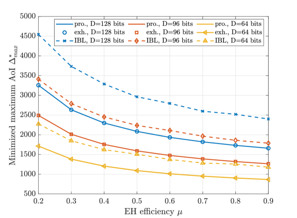
Figure 6: The minimized maximum of AoI among devices $\Delta^{*}_{\max}$ versus EH efficiency $\mu$ under various setups of $D=\{64,96,128\}$ bits. The results obtained by our proposed solution (solid lines) are compared with the results obtained by exhaustive search (markers), as well as the ones obtained with IBL solutions (dash lines).

Next, we show the advantage of our proposed solution by solving Problem (20) by comparing the results with two benchmarks. In particular, we plot the minimized maximum of AoI among devices $\Delta^{*}_{\max}$ versus EH efficiency $\mu$ under various setups of $D=\{64,96,128\}$ bits in Fig. 6. The results obtained by our proposed solution (indicated as pro.) are depicted with the solid line. Moreover, we also compare these results with two benchmarks, where the ones obtained by exhaustive search (indicated as exh.) are shown with a marker while ones obtained with IBL solutions (indicated as IBL) are plotted with a dash line.

As expected, $\Delta^{*}_{\max}$ reduces when we increase $\mu$, since higher $\mu$ indicates more harvested power. Therefore, it requires less charging duration $m_{c,i}$ to achieve the same level of error probability $\varepsilon_{i}$. Moreover, the improvement becomes flat when $\mu$ is already high due to the fixed received power. It should be pointed out that we may not observe the same behavior when increasing the transmit power $p_{c}$. This is due to the fact that the server is in the full-duplex mode and suffers from the self-interference, which also scales with $p_{c}$. We can also observe that our proposed solutions are able to achieve the same performance as the ones with the exhaustive search. However, since we solve Problem (20) via convex programming, the complexity is much lower. On the other hand, the AoI performance with IBL solutions, which ignores the influence of FBL codes, is significantly worse than our proposed solutions. In fact, as discussed in Fig. 4 and Fig. 5, to obtain the IBL solutions is to choose the scheduling policy so that $\log_{2}(1+\gamma_{i})=\frac{D}{m_{r,i}}$. Under the IBL assumption, it means that the AoI is minimized with no update error, i.e., $\varepsilon_{i}=0$. However, FBL model in (17) indicates that we have $\varepsilon_{i}=0.5$ if it holds $\log_{2}(1+\gamma_{i})=\frac{D}{m_{r,i}}$. Therefore, with FBL codes, if we simply adopt IBL model, the performance will be much worse. This motivates us to revisit the scheduling policy design with the consideration of FBL impact.

We also plot the minimized maximum of AoI among devices $\Delta^{*}_{\max}$ versus packet size $D$ under various setups of $\mu=\{0.3,0.6,0.9\}$ that are obtained by our proposed solutions, the exhaustive search, and with the IBL solutions in the similar style of Fig. 6, respectively. We also observe similar trends, i.e., $\Delta^{*}_{\max}$ increases if $D$ becomes large. Moreover, our proposed solutions can also achieve global optimality and outperform the results with IBL solutions. However, when $D$ is small, the gap between them becomes insignificant. This is due to the fact that the required power for a low error probability is also small. In fact, $\bar{\Delta}^{*}_{i}$ is dominated by $M$ if $\varepsilon_{i}$ approaches to $0$. Although this is also true for increasing $\mu$, its performance is still lower-bounded by the transmit power $p_{c}$.

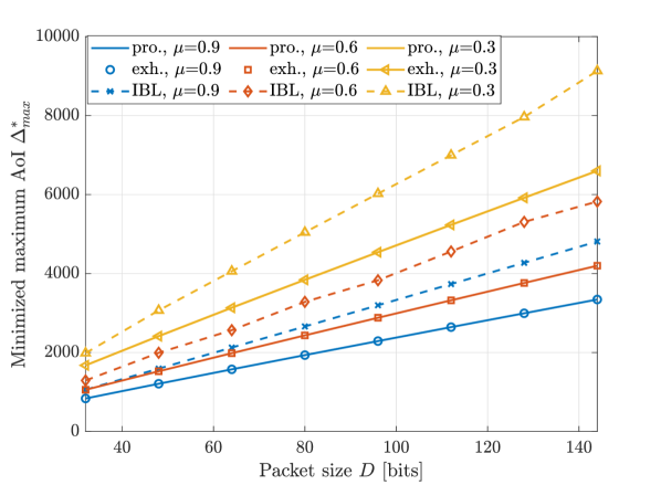
Figure 7: The minimized maximum of AoI among devices $\Delta^{*}_{\max}$ versus packet size $D$ under various setups of $\mu=\{0.3,0.6,0.9\}$. The results obtained by our proposed solution (solid lines) are compared with the results obtained by exhaustive search (markers), as well as the ones obtained with IBL solutions (dash lines).

VI-D Impact of Number of devices

In this subsection, we investigate the impact of the number of devices on the AoI performance and the role of cluster capacity in the system design. In particular, we plot the minimized maximum AoI $\Delta^{*}_{\max}$ (depicted as lines) and the optimal common charging duration $m^{*}_{c}$ (depicted as bars) versus the number of devices $I$ under various setups of distance $\bar{d}=\{1.4,1.5,1.6\}$ m in Fig 8. Moreover, for each setup, we indicate the cluster capacity $C_{\text{cap}}$ obtained with (28). For the sake of generality, in this figure, we consider that all devices are homogenous with the unified distance $\bar{d}$. When $I\leq C_{\text{cap}}$, $\Delta^{*}_{\max}$ is not influenced by $I$. This is due to the fact that the "free space", i.e., the common charging duration $m^{*}_{c}$ is non-zero. Therefore, the cluster is unsaturated and can support more devices. However, if we keep adding more devices so that $I>C_{\text{cap}}$, $\Delta^{*}_{\max}$ starts to grow. This is due to the fact that the cluster is now saturated with $m^{*}_{c}=0$. Clearly, the further distance of the devices is, the worse $\Delta^{*}_{\max}$ becomes. However, it means that $C_{\text{cap}}$ is also larger since the devices require more energy to carry out a reliable transmission with worse channel gain, i.e., larger $m^{*}_{c}$. In other words, the cluster can support more devices without influencing $\Delta^{*}_{\max}$. Therefore, as discussed in Section V, $C_{\text{cap}}$ is a metric related to each setup. Its absolute value does not directly indicate the AoI performance.

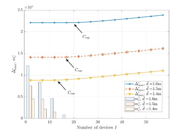
Figure 8: The minimized maximum AoI $\Delta^{*}_{\max}$ and the optimal common charging duration $m^{*}_{c}$ versus the number of devices $I$ under various setups of distance $\bar{d}=\{1.4,1.5,1.6\}$ m.

Since Fig. 8 shows the impact of the number of homogenous devices, it is also interesting to investigate the impact of adding different devices on the AoI performance. Therefore, we set $16$ homogenous devices with distance $\bar{d}=1.6$ m in the cluster, and add an additional devices $i_{\text{add}}$ with distance $d_{i_{\text{add}}}$. Then, we plot the minimized maximum AoI $\Delta_{\max}$ obtained via convex programming in Problem 20 versus $d_{i_{\text{add}}}$ in the top sub-figure of Fig. 9 while the common charging duration $m^{*}_{c}$ and update duration of the added device $m^{*}_{r,i_{\text{add}}}$ in the bottom sub-figure. Moreover, we also show the AoI obtained with Alg. 1 and the corresponding update duration $m^{\circ}_{i_{\text{add}}}$ in each sub-figure. Similar to the observation in Fig. 8, $\Delta_{\max}$ remains unchanged when it holds $d_{i_{\text{add}}}\leq\bar{d}$. It implies that the cluster is unsaturated. However, once the device $i_{\text{add}}$ becomes the furthest one in the cluster, $\Delta_{\max}$ increases. This is due to the fact that $m_{i_{\text{add}}}$ occupies more "free space" than the cluster could provide, which is demonstrated in the bottom sub-figure. Therefore, the AoI performance of the system is always lower-bounded by the AoI of the worse device. Moreover, we can observe that our proposed Algorithm in Alg. 1 is able to achieve the globally optimal solution, when the cluster is unsaturated. However, if the cluster becomes saturated, we lose the global optimality. That being said, the performance gap between our Algorithm and the optimal solution is acceptable when its distance is not far away from other devices, e.g., within $1$ m in our setups. Considering the significantly low complexity, it can still be applied in practical systems even when the cluster is saturated. This observation confirms the advantage of our algorithm.

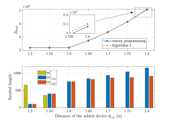
Figure 9: The minimized maximum AoI $\Delta_{\max}$, common charging duration $m^{*}_{c}$, and update duration $m^{*}_{r,i_{\text{add}}}$ versus the distance of added devices $d_{i_{\text{add}}}$ [m] with $16$ existing devices in the distance of $\bar{d}=1.6$ m. Both results from solving convex problem (20) and Alg. 1 are shown.

VII Conclusion

In this paper, we studied the potential of THz communication, with a particular focus on mURLLC networks with WPT-powered devices. We highlighted the importance of real-time data, using the AoI as a metric indicating the timeliness of data. We formulated a fairness-aware AoI minimization problem by optimizing their update scheduling with the consideration of the influence of FBL codes on the AoI. To simplify the problem, we establish an equivalent, less complex scheduling policy. Our analytical findings allowed us to efficiently reformulate and solve the problem as a convex one. Additionally, we introduced the concept of AoI-oriented cluster capacity, which answers the key question of how many devices can be supported in the network without affecting the AoI. Our numerical results validated our analytical findings and demonstrated the impact of different parameters, which may provide practical insights for the designs of future THz communications with mURLLC services.

Appendix A Proof of Lemma 2

First, we introduce an auxiliary function:

$$\omega_{i}=\sqrt{\frac{m_{r,i}}{V(\gamma_{i})}}(\mathcal{C}(\gamma_{i})-\frac{{\color[rgb]{0,0,0}D}}{m_{r,i}})ln2,$$ (29)

with which we have $\varepsilon_{i}=Q(\omega_{i})$. Then, we investigate the convexity of $\varepsilon_{i}$ with respect to each single variable. In particular, the second derivative of $\varepsilon_{i}$ with respect to $m_{c,i}$ is given by:

$$\begin{split}\frac{\partial^{2}\varepsilon_{i}}{\partial m_{c,i}^{2}}&=\underbrace{\frac{\partial^{2}\varepsilon_{i}}{\partial\omega_{i}^{2}}}_{\geq 0}\underbrace{\left(\frac{\partial\omega_{i}}{\partial m_{c,i}}\right)^{2}}_{\geq 0}+\underbrace{\frac{\partial\varepsilon_{i}}{\partial\omega_{i}}}_{\leq 0}\cdot\underbrace{\frac{\partial^{2}\omega_{i}}{\partial m_{c,i}^{2}}}_{\leq 0}\geq 0.\end{split}$$ (30)

The inequality holds since $\frac{\partial^{2}\varepsilon_{i}}{\partial\omega_{i}^{2}}={\color[rgb]{0,0,0}\frac{1}{\sqrt{2\pi}}\omega_{i}e^{-\frac{\omega_{i}^{2}}{2}}}$ and $\frac{\partial\varepsilon_{i}}{\partial\omega_{i}}={\color[rgb]{0,0,0}-\frac{1}{\sqrt{2\pi}}e^{-\frac{\omega_{i}^{2}}{2}}}$. Moreover, according to [36], we have $\frac{\partial^{2}\omega_{i}}{\partial m_{c,i}^{2}}=\frac{\partial^{2}\omega_{i}}{\partial\gamma^{2}}\left(\frac{\mu_{i}z^{2}_{i}P_{c}}{\sigma^{2}+h_{I}p_{c}}\right)^{2}\leq 0$. Hence, $\varepsilon_{i}$ is convex in $m_{c,i}$.

Similarly, the second derivative of $\varepsilon_{i}$ with respect to $m_{c,i}$ is given by:

$$\begin{split}\frac{\partial^{2}\varepsilon_{i}}{\partial m_{c,i}^{2}}&=\underbrace{\frac{\partial^{2}\varepsilon_{i}}{\partial\omega_{i}^{2}}}_{\geq 0}\underbrace{\left(\frac{\partial\omega_{i}}{\partial m_{c,i}}\right)^{2}}_{\geq 0}+\underbrace{\frac{\partial\varepsilon_{i}}{\partial\omega_{i}}}_{\leq 0}\cdot\frac{\partial^{2}\omega_{i}}{\partial m_{c,i}^{2}}.\end{split}$$ (31)

Then, we could have $\frac{\partial^{2}\varepsilon_{i}}{\partial m_{c,i}^{2}}\geq 0$, if it holds $\frac{\partial^{2}\omega_{i}}{\partial m_{c,i}^{2}}$. In fact, after some manipulations, we have

$$\begin{split}\frac{\partial^{2}\omega_{i}}{\partial m_{r,i}^{2}}&=b\cdot(a_{0}+a_{1}\gamma_{i}+a_{2}\gamma^{2}_{i}+a_{3}\gamma^{3}_{i}+a_{4}\gamma^{4}_{i}+a_{5}\gamma^{5}_{i})\\ &\triangleq b\cdot f(\gamma_{i}),\end{split}$$ (32)

where

$$a_{0} =12\ln 2r_{i}-36r_{i},$$ (33)

$$a_{1} =8-5\ln(1+\gamma_{i})-126r_{i}+39\ln 2r_{i},$$

$$a_{2} =20-162r_{i}-16\ln(1+\gamma_{i})+42ln2r_{i},$$

$$a_{3} =16-90r_{i}-18\ln(1+\gamma_{i})+12ln2r_{i},$$

$$a_{4} =4-8\ln(1+\gamma_{i})-18r_{i}-6ln2r_{i},$$

$$a_{5} =-\ln(1+\gamma_{i})-3\ln 2r_{i}.$$

Moreover, we have

$$b_{0}=\frac{\ln 2m^{6}_{r,i}}{4bm_{r,1}ln2(b+2m_{r,1})^{4}(\frac{m_{r,1}^{3}+2bm_{r,1}^{2}+b^{2}m_{r,1}}{b^{2}+2bm_{r,1}})^{3/2}}\geq 0,$$ (34)

where $b=\frac{z_{r,i}z_{c,i}u_{i}p_{c}m_{c,i}}{\sigma^{2}+h_{I}p_{c}}$ and $r_{i}=\frac{{\color[rgb]{0,0,0}D}}{m_{r,i}}$. Note that $f(\gamma_{i})$ is a polynomial. We can establish further inequalities to facilitate its expression:

$$a_{5}\gamma_{i}^{5}\leq(-\ln(1+\gamma_{i})-3\ln 2r_{i})\gamma_{i}^{2}$$ (35)

$$a_{4}\gamma^{4}_{i}\leq(4-8\ln(1+\gamma_{i})-18r_{i})\gamma_{i}^{2}-6\ln 2r_{i}\gamma_{i}$$ (36)

$$a_{3}\gamma_{i}^{3}\leq(16-18\ln(1+\gamma_{i})-87r_{i}+12\ln 2r_{i})\gamma_{i}^{3}-3r_{i}\gamma_{i}$$ (37)

Combing (35) - (37), we can reduce the order of $f$ with an inequality:

$$\begin{split}f(\gamma_{i})\leq\hat{a}_{3}\gamma_{i}^{3}+\hat{a}_{2}\gamma_{i}^{2}+\hat{a}_{1}\gamma_{i}+\hat{a}_{0}.\end{split}$$ (38)

Therefore, we have $f\leq 0$, if

$$\hat{a}_{3}=16-18ln(1+\gamma)-87r+12lnr\leq 0$$ (39)

$$\hat{a}_{2}=24-180r-25ln(1+\gamma)+39ln2r\leq 0$$

$$\hat{a}_{1}=8-129r-5ln(1+\gamma)+33ln2r\leq 0$$

$$\hat{a}_{0}=12ln2r-36r\leq 0.$$

As a result, $\varepsilon_{i}$ is convex in $m_{r,i}$ if $r_{i}\geq\frac{16-18ln(1+\gamma_{i})}{87-12ln2}\geq\frac{16-18ln2}{87-12ln2}=0.0449$

Next, we move on to the joint convexity. The Hessian matrix of $\varepsilon_{i}$ is given by:

$$\begin{gathered}\mathbf{H}=\begin{bmatrix}\frac{\partial^{2}\varepsilon_{i}}{\partial m_{r,i}^{2}}&\frac{\partial^{2}\varepsilon_{i}}{\partial m_{r,i}\partial m_{c,i}}\\ \frac{\partial^{2}\varepsilon_{i}}{\partial m_{c,i}\partial m_{r,i}}&\frac{\partial^{2}\varepsilon_{i}}{\partial m_{c,i}^{2}}\end{bmatrix}\end{gathered}$$ (40)

where

$$\frac{\partial^{2}\varepsilon_{i}}{\partial m_{r,i}\partial m_{c,i}}=\frac{\partial^{2}\varepsilon}{\partial\gamma^{2}}\frac{\partial\gamma}{\partial m_{c,i}}\frac{\partial\gamma}{\partial m_{r,i}}+\frac{\partial\varepsilon_{i}}{\partial\gamma}\frac{\partial\gamma}{\partial m_{c,i}\partial m_{r,i}},$$ (41)

$$\frac{\partial^{2}\varepsilon_{i}}{\partial m_{c,i}^{2}}=\frac{\partial^{2}\varepsilon_{i}}{\partial\gamma^{2}}(\frac{\partial\gamma}{\partial m_{c,i}})^{2}+\frac{\partial\varepsilon_{i}}{\partial\gamma}\frac{\partial^{2}\gamma}{\partial m_{c,i}^{2}}+\frac{\partial^{2}\varepsilon_{i}}{\partial m_{c,i}^{2}},$$ (42)

and

$$\frac{\partial^{2}\varepsilon_{i}}{\partial m_{r,i}^{2}}=\frac{\partial^{2}\varepsilon_{i}}{\partial\gamma^{2}}(\frac{\partial\gamma}{\partial m_{r,i}})^{2}+\frac{\partial\varepsilon_{i}}{\partial\gamma}\frac{\partial^{2}\gamma}{\partial m_{r,i}^{2}}+\frac{\partial^{2}\varepsilon_{i}}{\partial m_{r,i}^{2}}.$$ (43)

As we showed before, the upper-left element of $\mathbf{H}$ is non-negative. Moreover, its determinate can be written as:

$$\begin{split}\det[H]&=\frac{\partial^{2}\varepsilon_{i}}{\partial m_{c,i}^{2}}\frac{\partial^{2}\varepsilon_{i}}{\partial m_{r,i}^{2}}-(\frac{\partial^{2}\varepsilon_{i}}{\partial m_{r,i}\partial m_{c,i}})^{2}\\ &=\frac{\partial^{2}\varepsilon_{i}}{\partial\gamma_{i}^{2}}\frac{\partial^{2}\varepsilon_{i}}{\partial m_{r,i}^{2}}(\frac{\partial\gamma_{i}}{\partial m_{c,i}})^{2}-(\frac{\partial\varepsilon_{i}}{\partial\gamma_{i}}\frac{\partial\gamma_{i}}{\partial m_{r,i}\partial m_{c,i}})^{2}\\ &=\frac{P^{2}}{m_{r,i}^{2}\sigma_{s}^{4}}\bigg{(}\frac{\partial^{2}\varepsilon_{i}}{\partial\gamma_{i}^{2}}\frac{\partial^{2}\varepsilon_{i}}{\partial m_{r,i}^{2}}-\frac{\partial\varepsilon_{i}}{\partial\gamma_{i}}\frac{1}{m_{r,i}^{2}}\bigg{)}\\ &\geq\frac{P^{2}}{m_{r,i}^{2}\sigma_{s}^{4}}\bigg{(}\frac{\partial^{2}\varepsilon_{i}}{\partial\omega_{i}^{2}}(\frac{\partial\omega_{i}}{\partial\gamma_{i}})^{2}\frac{\partial\varepsilon_{i}}{\partial\omega_{i}}\frac{\partial^{2}\omega_{i}}{\partial m_{r,i}^{2}}-(\frac{\partial\varepsilon_{i}}{\partial\omega_{i}}\frac{\partial\omega_{i}}{\partial\gamma_{i}})^{2}\bigg{)}\\ &=\frac{P^{2}}{m_{r,i}^{2}\sigma_{s}^{4}}\bigg{(}\frac{\partial\omega_{i}}{\partial\gamma_{i}}\bigg{)}^{2}\frac{\partial\varepsilon_{i}}{\partial\omega_{i}}\frac{1}{\sqrt{2\pi}}e^{-\frac{\omega_{i}^{2}}{2}}\bigg{(}\omega_{i}\frac{\partial^{2}\omega_{i}}{\partial m_{r,i}^{2}}+\frac{1}{m_{r,i}^{2}}\bigg{)}\\ &=A\bigg{(}\sqrt{\frac{m_{r,i}}{V}}(C-\frac{{\color[rgb]{0,0,0}D}}{m_{r,i}})\\ &\leavevmode\nobreak\ \leavevmode\nobreak\ \leavevmode\nobreak\ \leavevmode\nobreak\ \cdot\big{(}-\frac{C}{4\sqrt{m_{r,i}^{3}V}}-\frac{3}{4}\frac{{\color[rgb]{0,0,0}D}}{m_{r,i}\sqrt{m_{r,i}^{3}V}}\big{)}ln2+\frac{1}{m_{r,i}^{2}}\bigg{)}\\ &\overset{V\leq 1,\varepsilon\leq 0.1}{\geq}A\bigg{(}1.25(-\frac{C}{4m_{r,i}}-\frac{3}{4}\frac{{\color[rgb]{0,0,0}D}}{m_{r,i}^{2}})ln2+\frac{1}{m_{r,i}^{2}}\bigg{)}\\ &\geq 0,\end{split}$$ (44)

where $A=\frac{P^{2}}{m_{r,i}^{2}\sigma_{s}^{4}}\bigg{(}\frac{\partial\omega_{i}}{\partial\gamma_{i}}\bigg{)}^{2}\frac{\partial\varepsilon_{i}}{\partial\omega_{i}}\frac{1}{\sqrt{2\pi}}e^{-\frac{\omega_{i}^{2}}{2}}\geq 0$. The last inequality holds if

$$\mathcal{C}m_{r,i}+3{\color[rgb]{0,0,0}D}\geq\frac{4}{\ln(2)}.$$ (45)

Hence, $\varepsilon_{i}$ is jointly convex in $m_{r,i}$ and $m_{c,i}$ if the condition (21) is fulfilled.

References

- [1] Y. Zhu, X. Yuan, B. Han, Y. Hu, and A. Schmeink, “Average Age-of-Information Minimization in EH-enabled Low-Latency IoT Networks,” in ICC 2021 - IEEE International Conference on Communications, 2021, pp. 1–6.
- [2] W. Jiang, Q. Zhou, J. He, M. A. Habibi, S. Melnyk, M. E. Absi, B. Han, M. Di Renzo, H. D. Schotten, F.-L. Luo, T. S. El-Bawab, M. Juntti, M. Debbah, and V. C. M. Leung, “Terahertz Communications and Sensing for 6G and Beyond: A Comprehensive View,” 2023. [Online]. Available: https://arxiv.org/abs/2307.10321
- [3] J. Huang, Y. Zhou, Z. Ning, and H. Gharavi, “Wireless Power Transfer and Energy Harvesting: Current Status and Future Prospects,” IEEE Wireless Communications, vol. 26, no. 4, pp. 163–169, 2019.
- [4] C. S. Lai, Y. Jia, Z. Dong, D. Wang, Y. Tao, Q. H. Lai, R. T. K. Wong, A. F. Zobaa, R. Wu, and L. L. Lai, “A Review of Technical Standards for Smart Cities,” Clean Technologies, vol. 2, no. 3, p. 290–310, Aug. 2020.
- [5] M. M. Islam, A. Rahaman, and M. R. Islam, “Development of Smart Healthcare Monitoring System in IoT Environment,” SN Computer Science, vol. 1, no. 3, May 2020.
- [6] L. Zhang, X. Bao, and W. Zhang, “Data Recovery of Sparse Sensors in Internet of Nano Things,” IEEE Internet of Things Journal, p. 1–1, 2023.
- [7] C. She, C. Sun, Z. Gu, Y. Li, C. Yang, H. V. Poor, and B. Vucetic, “A Tutorial on Ultrareliable and Low-Latency Communications in 6G: Integrating Domain Knowledge Into Deep Learning,” Proceedings of the IEEE, vol. 109, no. 3, pp. 204–246, 2021.
- [8] S. Dang, O. Amin, B. Shihada, and M.-S. Alouini, “What should 6G be?” Nature Electronics, vol. 3, no. 1, p. 20–29, Jan. 2020.
- [9] Y. Polyanskiy, H. V. Poor, and S. Verdu, “Channel Coding Rate in the Finite Blocklength Regime,” IEEE Trans. Inf. Theory, vol. 56, no. 5, pp. 2307–2359, 2010.
- [10] Y. Sun, E. Uysal-Biyikoglu, R. D. Yates, C. E. Koksal, and N. B. Shroff, “Update or Wait: How to Keep Your Data Fresh,” IEEE Transactions on Information Theory, vol. 63, no. 11, pp. 7492–7508, 2017.
- [11] D. C. Nguyen, M. Ding, P. N. Pathirana, A. Seneviratne, J. Li, D. Niyato, O. Dobre, and H. V. Poor, “6G Internet of Things: A Comprehensive Survey,” IEEE Internet of Things Journal, vol. 9, no. 1, pp. 359–383, 2022.
- [12] J. M. Jornet and I. F. Akyildiz, “Channel Modeling and Capacity Analysis for Electromagnetic Wireless Nanonetworks in the Terahertz Band,” IEEE Transactions on Wireless Communications, vol. 10, no. 10, pp. 3211–3221, 2011.
- [13] C. Han, A. O. Bicen, and I. F. Akyildiz, “Multi-Ray Channel Modeling and Wideband Characterization for Wireless Communications in the Terahertz Band,” IEEE Transactions on Wireless Communications, vol. 14, no. 5, pp. 2402–2412, 2015.
- [14] H. Elayan, C. Stefanini, R. M. Shubair, and J. M. Jornet, “Stochastic noise model for intra-body terahertz nanoscale communication,” in Proceedings of the 5th ACM International Conference on Nanoscale Computing and Communication. ACM, Sep. 2018. [Online]. Available: https://doi.org/10.1145/3233188.3233191
- [15] Y. Chen and C. Han, “Channel Modeling and Characterization for Wireless Networks-on-Chip Communications in the Millimeter Wave and Terahertz Bands,” IEEE Transactions on Molecular, Biological and Multi-Scale Communications, vol. 5, no. 1, pp. 30–43, 2019.
- [16] N. Akkari, P. Wang, J. M. Jornet, E. Fadel, L. Elrefaei, M. G. A. Malik, S. Almasri, and I. F. Akyildiz, “Distributed Timely Throughput Optimal Scheduling for the Internet of Nano-Things,” IEEE Internet of Things Journal, vol. 3, no. 6, pp. 1202–1212, 2016.
- [17] L. Feng, A. Ali, M. Iqbal, A. K. Bashir, S. A. Hussain, and S. Pack, “Optimal Haptic Communications Over Nanonetworks for E-Health Systems,” IEEE Transactions on Industrial Informatics, vol. 15, no. 5, pp. 3016–3027, 2019.
- [18] X.-W. Yao, C.-C. Wang, W.-L. Wang, and J. M. Jornet, “On the Achievable Throughput of Energy-Harvesting Nanonetworks in the Terahertz Band,” IEEE Sensors Journal, vol. 18, no. 2, pp. 902–912, 2018.
- [19] I. Krikidis, “Average Age of Information in Wireless Powered Sensor Networks,” IEEE Wireless Communications Letters, vol. 8, no. 2, pp. 628–631, 2019.
- [20] Q. Gu, G. Wang, R. Fan, F. Li, H. Jiang, and Z. Zhong, “Optimal Resource Allocation for Wireless Powered Sensors: A Perspective From Age of Information,” IEEE Communications Letters, vol. 24, no. 11, pp. 2559–2563, 2020.
- [21] L. Liu, K. Xiong, J. Cao, Y. Lu, P. Fan, and K. B. Letaief, “Average AoI Minimization in UAV-Assisted Data Collection With RF Wireless Power Transfer: A Deep Reinforcement Learning Scheme,” IEEE Internet of Things Journal, vol. 9, no. 7, pp. 5216–5228, 2022.
- [22] H. Ren, C. Pan, Y. Deng, M. Elkashlan, and A. Nallanathan, “Joint Power and Blocklength Optimization for URLLC in a Factory Automation Scenario,” IEEE Transactions on Wireless Communications, vol. 19, no. 3, pp. 1786–1801, 2020.
- [23] Q. Peng, H. Ren, C. Pan, N. Liu, and M. Elkashlan, “Resource Allocation for Uplink Cell-Free Massive MIMO Enabled URLLC in a Smart Factory,” IEEE Transactions on Communications, vol. 71, no. 1, pp. 553–568, 2023.
- [24] C. Li, C. She, N. Yang, and T. Q. S. Quek, “Secure Transmission Rate of Short Packets With Queueing Delay Requirement,” IEEE Transactions on Wireless Communications, vol. 21, no. 1, pp. 203–218, 2022.
- [25] X. Zhang, J. Wang, and H. V. Poor, “Optimal Resource Allocations for Statistical QoS Provisioning to Support mURLLC Over FBC-EH-Based 6G THz Wireless Nano-Networks,” IEEE Journal on Selected Areas in Communications, vol. 39, no. 6, pp. 1544–1560, 2021.
- [26] R. D. Yates, Y. Sun, D. R. Brown, S. K. Kaul, E. Modiano, and S. Ulukus, “Age of Information: An Introduction and Survey,” IEEE Journal on Selected Areas in Communications, vol. 39, no. 5, pp. 1183–1210, 2021.
- [27] F. Afsana, S. A. Mamun, M. S. Kaiser, and M. R. Ahmed, “Outage capacity analysis of cluster-based forwarding scheme for Body Area Network using nano-electromagnetic communication,” in 2015 2nd International Conference on Electrical Information and Communication Technologies (EICT), 2015, pp. 383–388.
- [28] J. M. Jornet and I. F. Akyildiz, “Joint Energy Harvesting and Communication Analysis for Perpetual Wireless Nanosensor Networks in the Terahertz Band,” IEEE Transactions on Nanotechnology, vol. 11, no. 3, pp. 570–580, 2012.
- [29] Y. Hu, X. Yuan, T. Yang, B. Clerckx, and A. Schmeink, “On the Convex Properties of Wireless Power Transfer With Nonlinear Energy Harvesting,” IEEE Transactions on Vehicular Technology, vol. 69, no. 5, pp. 5672–5676, 2020.
- [30] R. Zhang, K. Yang, Q. H. Abbasi, K. A. Qaraqe, and A. Alomainy, “Analytical Modelling of the Effect of Noise on the Terahertz In-Vivo Communication Channel for Body-centric Nano-networks,” Nano communication networks, vol. 15, pp. 59–68, 2018.
- [31] Y. Polyanskiy, H. V. Poor, and S. Verdu, “Dispersion of Gaussian Channels,” in 2009 IEEE ISIT, 2009, pp. 2204–2208.
- [32] B. Han, Y. Zhu, Z. Jiang, M. Sun, and H. D. Schotten, “Fairness for Freshness: Optimal Age of Information Based OFDMA Scheduling With Minimal Knowledge,” IEEE Transactions on Wireless Communications, vol. 20, no. 12, pp. 7903–7919, 2021.
- [33] Y. Hu, Y. Zhu, M. C. Gursoy, and A. Schmeink, “SWIPT-Enabled Relaying in IoT Networks Operating With Finite Blocklength Codes,” IEEE Journal on Selected Areas in Communications, vol. 37, no. 1, pp. 74–88, 2019.
- [34] J. Cao, X. Zhu, Y. Jiang, Z. Wei, and S. Sun, “Information Age-Delay Correlation and Optimization With Finite Block Length,” IEEE Transactions on Communications, vol. 69, no. 11, pp. 7236–7250, 2021.
- [35] S. P. Boyd and L. Vandenberghe, Convex optimization. Cambridge university press, 2004.
- [36] Y. Zhu, Y. Hu, X. Yuan, M. C. Gursoy, H. V. Poor, and A. Schmeink, “Joint Convexity of Error Probability in Blocklength and Transmit Power in the Finite Blocklength Regime,” IEEE Transactions on Wireless Communications, vol. 22, no. 4, pp. 2409–2423, 2023.