Convergence of overlapping domain decomposition methods with PML transmission conditions applied to nontrapping Helmholtz problems
Abstract
We study overlapping Schwarz methods for the Helmholtz equation posed in any dimension with large, real wavenumber and smooth variable wave speed. The radiation condition is approximated by a Cartesian perfectly-matched layer (PML). The domain-decomposition subdomains are overlapping hyperrectangles with Cartesian PMLs at their boundaries. The overlaps of the subdomains and the widths of the PMLs are all taken to be independent of the wavenumber.
For both parallel (i.e., additive) and sequential (i.e., multiplicative) methods, we show that after a specified number of iterations – depending on the behaviour of the geometric-optic rays – the error is smooth and smaller than any negative power of the wavenumber. For the parallel method, the specified number of iterations is less than the maximum number of subdomains, counted with their multiplicity, that a geometric-optic ray can intersect.
These results, which are illustrated by numerical experiments, are the first wavenumber-explicit results about convergence of overlapping Schwarz methods for the Helmholtz equation, and the first wavenumber-explicit results about convergence of any domain-decomposition method for the Helmholtz equation with a non-trivial scatterer (here a variable wave speed).
1 Introduction
1.1 Informal description of the problem
We consider the following Helmholtz problem: for arbitrary , given , (normalised) strictly-positive wavespeed with compact, and wavenumber , find satisfying the Helmholtz equation and Sommerfeld radiation condition:
| (1.1) |
Since is unbounded, a standard approximation to this Helmholtz problem is to truncate the domain at an artificial boundary chosen so that the truncated domain contains both and (i.e., the scatterer and the data) and approximate the radiation condition by a perfectly-matched layer (PML) [3]. In this paper we assume that the artificial boundary is a hyperrectangle, and that the PML is a Cartesian PML (i.e., the scaling is active in Cartesian coordinate directions; see §1.4.2 below for a precise definition).
Helmholtz solutions oscillate on a length scale of , and approximating an arbitrary function oscillating on this scale requires degrees of freedom, where is the length scale of the domain. For piecewise polynomials of fixed degree, the number of degrees of freedom required is because of the pollution effect [1, 21]. The linear systems resulting from finite-element discretisations of (1.1) are therefore very large. Furthermore, since the standard variational formulation of the Helmholtz problem above is not self-adjoint and not coercive, methods that work well for self-adjoint coercive problems, such as Poisson’s equation, usually perform very badly for Helmholtz problems (see, e.g., the review [18]).
Domain-decomposition (DD) methods approximate the solution of the Helmholtz problem on the computational domain by solving Helmholtz problems on subdomains (either overlapping or non-overlapping) of the original domain, with each subdomain problem involving fewer degrees of freedom than the original problem. Each iteration of a parallel (a.k.a. additive) method involves solving decoupled problems on each subdomain (i.e., subdomains do not communicate with each other at this stage). In contrast, each iteration of a sequential (a.k.a. multiplicative) method involves communication between subdomains at each solve phase.
1.2 Context: DD methods using PML
The design and analysis of DD methods for solving the Helmholtz equation is a very active area; see, e.g., the reviews [17, 18, 33, 25, 23].
A key question is: what boundary conditions should be imposed on the DD subdomains? It is known that the optimal boundary condition on a particular DD subdomain is the Dirichlet-to-Neumann map for the Helmholtz equation posed in the exterior of that subdomain (as a subset of the whole domain) [42, §2] [16, §2], [12, §2.4]. However, complete knowledge of these maps is equivalent to knowing the solution operator for the original problem. The design of good, practical subdomain boundary conditions is then the goal of optimised Schwarz methods; see, e.g., [22].
Using PML as a subdomain boundary condition for Helmholtz DD was first advocated for in [54], and there are now many DD methods for Helmholtz using PML on subdomain boundaries with impressive empirical performance; see, e.g., [15, 52, 10, 58, 53, 35, 47, 5] and the reviews [25, 23].
It is now understood in a -explicit way how PML approximates the Dirichlet-to-Neumann map associated with the Sommerfeld radiation condition. Indeed, when and , the error between the true Helmholtz solution and the Cartesian PML approximation decreases exponentially in , the width of the PML, and the strength of the scaling by [10, Lemma 3.4] (this result also holds for general scatterers in with a radial PML by [20]). For general smooth and any , this error is smaller than any negative power of by Theorem 4.6 below.
However, there is no rigorous understanding of how well PML approximates the (more complicated) Dirichlet-to-Neumann maps corresponding to the optimal DD boundary conditions for general decompositions and non-trivial scatterers; i.e., there are no rigorous -explicit results about the convergence of DD methods using PML applied to Helmholtz problems with and non-trivial scatterers.
The only existing -explicit rigorous convergence results are for the sequential “source transfer” DD methods (which [25] showed can be considered as a particular type of optimised Schwartz method) applied to (1.1) with (i.e., no scattering). These methods involve subdomains that only overlap via the perfectly-matched layers (i.e., the physically-relevant parts of the subdomains do not overlap). For these methods applied to (1.1) with (i.e., no scattering), -explicit convergence of the DD method at the continuous level can be obtained from a -explicit result about how well (Cartesian) PML approximates the Sommerfeld radiation condition – this is precisely because the optimal boundary conditions on the subdomains in this case are the Dirichlet-to-Neumann maps associated with the Sommerfeld radiation condition. Therefore, accuracy of Cartesian PML when [10, Lemma 3.4] is then the heart of the -explicit convergence proofs of the source-transfer-type methods in [10, 35, 13, 36, 37] for .
1.3 Informal description of the main results
The main results of the present paper, Theorems 1.1-1.4 and 1.6 below, concern both parallel and sequential overlapping Schwarz methods at the PDE level (i.e., before discretisation).
Theorem (Informal summary of Theorems 1.1-1.4 and 1.6).
For both parallel and sequential overlapping Schwarz methods applied to the Cartesian PML approximation of (1.1), where the subdomains are hyperrectangles with Cartesian PMLs at their boundaries, the following is true. After a number of iterations depending on the behaviour of the geometric-optic rays, given any there exists such that the error is smooth and smaller than for all .
In particular, this implies that the fixed-point iterations converge exponentially quickly in the number of iterations for sufficiently-large .
These results are the first -explicit results about convergence of overlapping Schwarz methods for the Helmholtz equation, and the first -explicit results about convergence of any DD method for the Helmholtz equation with a non-trivial scatterer (here a variable wave speed). We highlight the following.
-
•
These results are valid on fixed domains for sufficiently-large , i.e., the PML widths and DD overlaps are arbitrary, but independent of . Obtaining results that are also explicit in these geometric parameters of the decomposition will require more technical arguments than those used here.
-
•
We make clear exactly what properties of PML are required to obtain these results, and for what other complex absorption operators these results also hold (see Appendix A).
- •
1.4 Definition of the overlapping Schwarz methods considered in this paper
1.4.1 Definition of the subdomains
Let the -dimensional hyperrectangular domain be given by the Cartesian product
Let be an overlapping decomposition of in hyperrectangular subdomains:
| (1.2) |
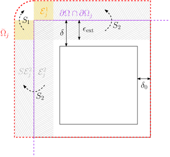
We extend and each , , by adding a PML layer to each, to form the domains and . Namely, let and denote respectively the PML width on and the interior PML width and let
where if the corresponding edge of belongs to the interior of , and otherwise; i.e., edges of subdomains that touch the boundary have the same PML width as (i.e., ), and interior subdomain edges have PML width which can be different than .
1.4.2 The scaled operators
We now define standard Cartesian PMLs of width at the boundary of and width at the boundary of each . For simplicity, we assume that the same PML scaling function is used inside every PML; however, this assumption can be easily removed, with, say, one function used in the PMLs of width and another used in the PMLs of width , at the cost of introducing more notation.
Let (with subscript standing for “scaling”) be such that
for some (observe that is then linear for ). (This assumption is to avoid technical issues about propagation of singularities – see Remark 2.5 below.)
For any , we define the following scaling functions in the -direction by
and similarly, the subdomain scaling functions in the -direction for by
We now define the scaled operators and by
and
| (1.3) |
Given that is strictly positive and such that , let
| (1.4) |
These operators are defined on , but we consider as a operator , and as an operator . If Dirichlet boundary data in is prescribed on the corresponding boundaries, these operators are then invertible.
In the proofs of our main results, a key region is the following subset of :
is the part of the PML region of where the PML in differs from the PML in (i.e., where ). Note that when is an interior subdomain, .
1.4.3 The Helmholtz problem
Given , find such that
| (1.5) |
The solution exists and is unique either for fixed when the PML width is sufficiently large [30, Theorem 5.5], [6, Theorem 5.7] or for fixed and scaling function when is sufficiently large (by Lemma 4.5 below). When and , [10, Lemma 3.4] shows that the error between and the solution of the true Helmholtz problem in satisfying the Sommerfeld radiation condition decays exponentially in and . Theorem 4.6 below shows that, for and , for fixed , this error is ; i.e., smaller than any negative power of .
1.4.4 The partition of unity
Let be a partition of unity subordinate to , i.e., is a family of non-negative elements of such that
| (1.6) |
and, additionally, in a neighbourhood of , each does not vary in the normal direction to the boundary of (this last assumption is for technical reasons, and can easily be achieved in practice).
1.4.5 The parallel overlapping Schwarz method
Given , for and any , let be the solution to
| (1.7) |
and then set
| (1.8) |
(where the subscript indicates that these are the iterates for the parallel/additive method).
Another way to write this is to introduce the local corrector , which satisfies
| (1.9) |
From this we see that the solution of (1.5) is a fixed point of (1.7)-(1.8). Indeed, if then by uniqueness of the PML problem on , and thus . (Note that the subdomain problems for are wellposed by the same results that ensure wellposedness of (1.5).)
In §8.1 below, we show that, on the discrete level, this parallel method can be understood as a natural PML-variant of the well-known RAS (restricted additive Schwarz) method.
1.4.6 The sequential overlapping Schwarz methods
The following sequential methods are designed to be used when the subdomains have certain additional structure (see the definitions of “strips” and “checkerboards” in §1.4.7 below), but can be written abstractly for any set of subdomains as follows.
Forward-backward sweeping. Given , let Then, for ,
-
1.
(Forward sweeping) For , let be the solution to
(1.10) where
Then set
(1.11) (where the subscript indicates that these are the iterates for a sequential/multiplicative method).
-
2.
(Backward sweeping) For , let be the solution to
where
Then set
(1.12)
Observe that the algorithm only uses the local approximations ; i.e., is not directly used to define . However, the approximation to the solution of (1.5) at each step is , obtained by combining the local approximations via the partition of unity in (1.11)/(1.12).
In forward-backward sweeping, the subdomains are always visited in the same order and its reverse. Some of our results about the sequential method involve changing the order in which the subdomains are visited from iteration to iteration, as described as follows.
General sequential method. Let be a sequence of permutations . For each , corresponds to the order that that subdomains are visited in the th sweep; e.g., is the first subdomain visited on the th sweep, is the second subdomain visited on the th sweep, etc. We therefore call a sequence of orderings.
We highlight immediately that forward-backward sweeping is defined by (i.e., odd-numbered sweeps visit the subdomains in order, and then even-numbered sweeps visit the subdomains in reverse order).
Given , let . Then for , for , let be the solution to
| (1.13) |
where
Then set
1.4.7 Strips and checkerboards
For , , we say that is a checkerboard of size if the following hold.
-
(i)
For , there exist
such that
with each of the form for some , .
-
(ii)
The overlapping decomposition of comes from extending each in each coordinate direction (apart from at ).
-
(iii)
The extensions in (ii) are such that, for all , overlaps only with , where and are extensions of adjacent nonoverlapping subdomains.
We say that is a -checkerboard if i.e. is the effective dimensionality of the checkerboard.
We say that is a strip if it is a -checkerboard. To simplify notation, we then assume that the subdomains of a strip are ordered monotonically (i.e., so that only overlaps and ).
Figure 1.1 shows an example of the grid formed by the points that is used in the definition of a particular -checkerboard of size , along with a particular subdomain .
1.5 Statement of the results about strips with
Theorem 1.1 (, strip, parallel method).
Assume that and that is a strip. Then, for any , there exists such that the following is true for any and . If is the solution to (1.5), and is a sequence of iterates for the parallel overlapping Schwarz method, then
The norm appearing in Theorem 1.1 is defined for by
| (1.14) |
and for by interpolation; i.e., is the standard norm on except that every derivative is weighted by (using this norm is motivated by the fact that Helmholtz solutions oscillate at frequency approximately ).
Theorem 1.2 (, strip, forward-backward sweeping).
Assume that and that is a strip. Then, for any , there exists such that the following is true for any and . If is the solution to (1.5), and is a sequence of iterates for the forward-backward sweeping overlapping Schwarz method, then
(i.e., after one forward and one backward sweep, the error is ).
1.6 Statement of the results about checkerboards with
Theorem 1.3 (, checkerboard, parallel method).
Assume that and that is a -checkerboard of size (with for all ). Then, for any , there exists such that the following is true for any and . If is the solution to (1.5), and is a sequence of iterates for the parallel overlapping Schwarz method, then
Theorem 1.3 contains Theorem 1.1 by recalling that a strip is a -checkerboard (with subdomains), and setting in Theorem 1.3.
To state the result for the sequential method on the checkerboard, we need the following notion. Informally, we say that a sequence of orderings is exhaustive if (i) given any ordering in the sequence, the sequence also contains the reverse ordering (i.e., where the subdomains are visited in reverse order), and (ii) given any directed straight line, there exists such that, in the order of subdomains corresponding to the ordering , the subdomains intersected by the straight line are visited in that order (but not necessarily one after the other) in that sweep. For the precise definition of exhaustive, see Definition 7.2 below.
For example, one forward sweep and one backward sweep on a strip corresponds to the ordering with , ; this ordering is exhaustive, since (i) the backward sweep is the reverse of the forward sweep (and vice versa), and (ii) any straight line that intersects more than one subdomain intersects them in the order they appear either in the forward sweep or in the backward sweep.
Examples 7.3 and 7.4 below describe how to easily construct exhaustive orderings of size for a -checkerboard. In particular, one can take corresponding to lexicographic order with respect to every vertex; see Figure 1.2. Lemma 7.5 shows that an exhaustive sequence of orderings for a -checkerboard must contain at least orderings.
| 7 | 8 | 9 |
|---|---|---|
| 4 | 5 | 6 |
| 1 | 2 | 3 |
| 9 | 8 | 7 |
|---|---|---|
| 6 | 5 | 4 |
| 3 | 2 | 1 |
| 1 | 2 | 3 |
|---|---|---|
| 4 | 5 | 6 |
| 7 | 8 | 9 |
| 3 | 2 | 1 |
|---|---|---|
| 6 | 5 | 4 |
| 9 | 8 | 7 |
Theorem 1.4 (, checkerboard, sequential method).
Assume that and that is a -checkerboard. Then, for any , there exists such that the following is true for any and . If is the solution to (1.5), and is a sequence of iterates for the general sequential overlapping Schwarz method following an exhaustive sequence of orderings of size , then
In particular, we can construct orderings (via Examples 7.3 and 7.4) so that
Remark 1.5 (Comparing the number of solves for the parallel and sequential methods on a checkerboard).
1.7 Statement of the most general result about the parallel method
We first recall the definition of the geometric-optic rays associated with the Helmholtz equation (1.1). Let and let
Given initial data , let be the solution of Hamilton’s equations
| (1.15) |
with initial conditions and ; we call such solutions trajectories of the flow associated to . The geometric-optic rays are then the spatial projections of the trajectories, i.e., their projections in the -variable. Observe that, when , the solution of (1.15) is just straight line motion , . Observe also the time reversibility property that if is a solution to (1.15) then so is .
The operator is non-trapping if, given there exists such that, the -projection of any trajectory starting in has left this set by time ; see, e.g., [34, Page 278]. (Strictly this is the definition of being non-trapping forward in time, but, due to time reversibility, this is equivalent to being non-trapping backward in time.)
Theorem 1.6 below depends on a quantity that depends on the properties of the trajectories. A precise definition of is given in §6.1 below (see also the informal discussion in §2.2), but, informally, we consider trajectories for the flow associated to travelling from the PML region of one subdomain to the PML region of another subdomain, and so on. is then the maximum number of subdomains, counted with their multiplicity, that any such trajectory can travel between. Importantly, when is nontrapping.
Theorem 1.6 (General , arbitrary hyperrectangular subdomains, parallel method).
Assume that is non-trapping. Then, for any , there exists such that the following is true for any and . If is the solution to (1.5), and is a sequence of iterates for the parallel overlapping Schwarz method, then
When , for a strip, Theorem 1.1 follows from Theorem 1.6 by showing that , and, for a checkerboard, Theorem 1.3 follows from Theorem 1.6 by showing that ; see §7.3 below.
When , the quantity can, in principle, be calculated from its definition (Definition 2.3) using ray tracing.
Remark 1.7 (The relationship of PML to the optimal subdomain boundary conditions).
Recall from §1.2 that the optimal boundary condition on a particular DD subdomain is the Dirichlet-to-Neumann map for the Helmholtz equation posed in the exterior of that subdomain (as a subset of the whole domain); in particular, the parallel overlapping Schwarz method with a strip decomposition with subdomains converges in iterations with these boundary conditions by [42, Proposition 2.4] and [16, Lemma 2.2].
Theorem 1.1 shows that when the parallel method with a strip decomposition with PML at the subdomain boundaries has error after iterations; i.e., PML approximates well the optimal boundary condition in this case.
When , Theorem 1.6 proves that the parallel method with a strip decomposition has error after iterations; we highlight that can be much larger than when and the rays are not straight lines (e.g., if the rays “turn around” at one end of the domain), and PML does not approximate well the optimal boundary condition in this case. The fact that PML at a subdomain boundary condition cannot take into account scattering occurring outside that subdomain was highlighted in [24, §4] and [25, §10].
2 Outline of how the main results are proved
§2.1-§2.4 explain the ideas behind the results for the parallel method (i.e., Theorems 1.1, 1.3, and 1.6). §2.5 and §2.6 then explain the results for the sequential methods (Theorem 1.2 and 1.4).
2.1 The error propagation matrix for the parallel method
For any and , we define the global and local errors
| (2.1) |
These definitions, the definition of the iterate (1.8), and the fact that is a partition of unity (1.6) imply that
| (2.2) |
We introduce the notation
| (2.3) |
We can interpret , after extension by zero from , as an element of , since is zero on and on . We call the local physical error. We highlight that the fact that is expressed in (2.3) in terms of and not the whole local error is expected, since contains contributions from the PML layers of that are not PML layers of , and hence not part of the original PDE problem (1.5) (and hence “unphysical”).
For and let be the solution to
| (2.4) |
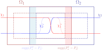
For technical reasons, we need a set of cut-off functions that have bigger support than the s. Let be such that, for each , , and on (recall that for an interior subdomain); such exist since the distance between and is as a consequence of and begin closed. The functions and are illustrated in the simple case of two subdomains (i.e, ) in Figure 2.1.
We define the physical error propagation matrix as
| (2.5) |
and, for any , the physical errors vector as
Lemma 2.1 (Physical error propagation for the parallel method).
and
| (2.6) |
2.2 Relating powers of to trajectories of the flow defined by
By (2.6), . By the definition of (2.5), powers of involve compositions of the maps , and these compositions applied to can be interpreted as the error travelling from subdomain to subdomain through the iterations.
The key ingredient to the proof of Theorem 1.6 is Lemma 2.4 below, which relates compositions of to properties of the trajectories of the flow travelling between the relevant subdomains.
We now introduce notation to describe trajectories travelling from subdomain to subdomain. Let be the set of finite sequences of elements of (i.e., the indices of subdomains) such that, for any , for all (i.e., the th component of corresponds to a different subdomain than the th component). We call the elements of words.
Definition (Informal statement of Definition 6.1 (following a word)).
A trajectory for the flow associated to follows a word of length if it passes through, in order, by going through the following sets
| (2.7) |
We make the following immediate remarks:
-
•
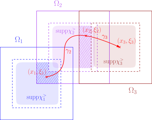
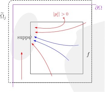
Figure 2.2 illustrates a trajectory following a word involving three subdomains of that do not touch the boundary.
- •
-
•
is the part of the PML of that intersects ; because is zero on the support of , the sets in (2.7) are disjoint.
-
•
A trajectory can follow more than one word because of the overlap of the subdomains.
The flow associated to only allows passage between certain sequences of subdomains. For example, if the , the trajectories of the flow are straight lines, and thus, since the subdomains are hyperrectangles, in a strip domain there is no trajectory following the word . To see this, consider the analogue of Figure 2.2 with the subdomain in the same horizontal strip as and ; in this modified diagram, a straight-line trajectory cannot leave the blue hatched area, go to the purple hatched area, and then come back to the blue hatched area.
Definition 2.2.
A word is allowed if there exists a trajectory for that follows .
Definition 2.3.
| (2.8) |
Since the sets in (2.7) are compact and disjoint, the assumption that is nontrapping implies that the length of allowed words is bounded above, ie .
For any of length , we define the composite map
| (2.9) |
The presence of the cut-offs in the definition of (2.5) means that is zero unless and overlap for all .
The heart of the proof of Theorem 1.6 is the following lemma.
Lemma 2.4.
| (2.10) |
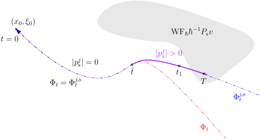
We show in §6.2 that Lemma 2.4 reduces to the following result, which describes precisely how, in the limit, the error travels from subdomain to subdomain through the iterations. The lemma is stated in phase space , where is position and is momentum; note that can be thought of as a Fourier variable measuring the direction of oscillation.
Lemma (Informal statement of Lemma 6.2).
For any , in the limit, is non-negligible (i.e., not ) only at points in phase space that are end points of trajectories that follow the word .
Lemma 6.2 is in turn proved using the following propagation result.
Lemma (Informal statement of Lemma 4.1).
Let be the solution to
If is nontrapping, then, in the limit, is non-negligible only at points in phase space that come from the data under the flow associated to .
Lemma 4.1 is stated rigorously and proved in §4, and we give the main ideas behind its proof in §2.3 below. Lemma 6.2 is stated in §6.2, and proved in §6.3. The idea is the following.
Sketch proof of Lemma 6.2 using Lemma 4.1.
Given , by the definitions of (2.5) and (2.4), equals multiplied by a Helmholtz solution on with data . Therefore, Lemma 4.1 shows that, in the limit, the mass of in phase space comes only from , i.e., the first domain in (2.7). (This concept of “mass in phase space” is made precise by the notion of wavefront set; see Definition B.6 below.)
Similarly, satisfies a Helmholtz problem on with data
. Therefore, Lemma 4.1 shows that, in the limit, the mass of comes only from the mass in that in turn came from .
In the same way, only contains mass that propagates between subdomains following the word , i.e., the subdomains listed in (2.7). ∎
2.3 Sketch proof of the propagation result (Lemma 4.1)
The two main concepts from semiclassical analysis used in the proof of Lemma 4.1 are the following.
-
1.
Propagation of singularities, used in the form that the absence of mass (in phase space) of the solution of propagates forwards along the flow defined by as long as the trajectory does not intersect the data (see Lemma B.11 below) and the imaginary part of the principal symbol of is non-positive.
- 2.
Since is elliptic in the directions that the scaling of the PML takes place (Lemma 3.5),
-
3.
A trajectory cannot exit without passing through a point where is elliptic (Lemma 4.4).
We now face the issue that the assumptions and conclusions of Lemma 4.1 involve the flow for (since this is the flow with physical relevance), but to prove the lemma we need to use propagation of singularities in the flow defined by (since Lemma 4.1 is all about solutions of ), and these two flows are different. The resolution of this apparent difficulty is that
-
4.
The flow defined by equals the flow defined by as long as it doesn’t reach a point where is elliptic (Lemma 4.2).
By the assumption that is nontrapping, any trajectory exits the domain; combining this with Points 3 and 4 we obtain
-
5.
Any point in is the endpoint of a trajectory of coming either from an elliptic point without intersecting the data, or comes from the data.
Point 5 combined with Point 2 implies that trajectories of coming from an elliptic point without intersecting the data carry no mass. Therefore Point 5 combined with Point 1 implies the result; i.e., that the solution contains mass only on points in phase space that come from the data under the flow associated to (this is illustrated graphically in Figure 4.2, next to the proof of Lemma 4.1).
Remark 2.5 (Why we assume that is linear near the PML boundary).
The principal symbol of the scaled operator has a negative imaginary part; see (3.4) below. For such an operator, the relevant propagation of singularities results in the semiclassical calculus for domains with a boundary have not yet been written down in the literature. Indeed, the relevant propagation of singularities results in the semiclassical calculus has been proved (i) on manifolds without boundary for operators with symbols whose imaginary parts are single-signed [14, Theorem E.47] (see Lemma B.10 below) and (ii) on manifolds with boundary for [57].
The assumption that is linear near the PML boundary allows us to use a reflection argument (similar to that used for the Cartesian PML analyses in 2-d in [6, Proof of Theorem 5.5], [10, Lemma 3.4]) to extend the solution past and use the propagation results of (i) above, i.e., bypassing the issue of propagation up to the boundary (exactly where in the proofs of the main results we do this is highlighted in Remark 6.3 below). Once the relevant propagation results are written down in the literature, this assumption can be removed.
Remark 2.6.
(Why we do not have a variable coefficient in the highest-order term of the PDE.) There is also large interest in solving the Helmholtz equation with a variable coefficient in the highest-order term; i.e., the PDE
| (2.11) |
where is a symmetric-positive-definite-matrix-valued function with . When and satisfies the Sommerfeld radiation condition, the solution of this problem is well-approximated by Cartesian PML. Indeed, Theorem 4.6 below holds verbatim: since when the PML is active, the imaginary part of the principal symbol is unaffected and propagation of singularities (as described informally in Point 1 above) still holds.
However, the analogue of the domain-decomposition methods defined in §1.4 for the PDE (2.11) involve local problems with the operator
| (2.12) |
where
(compare to (1.4) and (1.3)). For general , the imaginary part of the principal symbol of (2.12) no longer has a sign, and propagation of singularities does not hold. This is more than just a technical problem with the proofs: the numerical experiments in §8.5 give an example of a simple for which the PDE (2.11) is well posed, but the parallel Schwarz method applied to (2.11) with local problems involving (2.12) diverges.
2.4 Summary of the three ingredients used in the proof of Theorem 1.6 (the result about the parallel method)
- 1.
-
2.
Semiclassical analysis, showing that if is not allowed – Lemma 2.4.
-
3.
Properties of the trajectories of the flow associated with , dictating which are allowed.
All the discussion in this section has so far been about the parallel method. However, the three ingredients above show that to prove results about different methods, such as the sequential methods in §1.4.6, we only need to understand Point 1, i.e., the algebra of the error propagation, and then check whether the words appearing in the products are allowed or not. In the next subsection we illustrate this process for forward-backward sweeping on a strip when (i.e., the geometric-optic rays are straight lines).
2.5 Error propagation for forward-backward sweeping on a strip (i.e., the idea behind the proof of Theorem 1.2)
We now seek the sweeping analogue of the parallel error propagation result of Lemma 2.1. To do this, we set up notation for the error analogous to that used for the parallel method in §2.1.
Let be a sequence of iterates for the forward-backward sweeping defined in §1.4.6. Let
| (2.13) |
(with the subscript indicating that this is the error for the multiplicative/sequential method). We define the localised physical error by
| (2.14) |
(in exact analogue with (2.3)), Finally, we define the physical errors vector by
For any set of subdomains, for all – this follows from the definitions of (2.5) and (2.4) and the fact that where is supported. Therefore
| (2.15) |
where is lower triangular and is upper triangular, both with zero on the diagonal.
Lemma 2.7 (Error propagation for forward-backward sweeping).
For forward-backward sweeping, for ,
| (2.16) |
In the parallel case, Lemma 2.1 gives us immediately that . We now seek the analogue of this for forward-backward sweeping (see (2.18) below), using the additional structure of and when is a strip (in the sense of §1.4.7).
Lemma 2.8.
If is a strip then
| (2.17) |
Proof.
By definition of the partition of unity for a strip decomposition, and the “slightly bigger” set of cut-offs , if , then on . Thus if , and the result (2.17) follows. ∎
Proof of Theorem 1.2 using Lemma 2.4.
By the first equation in (2.16) with ,
hence, since ,
Similarly, by the second equation in (2.16) and then the above,
| (2.18) |
By Lemma 2.8, all the entries of consist of for some . Therefore, all the entries of any product of matrices appearing in the second sum in (2.18) are of the form , where and (and is empty if and in the sum).
We have now completed the analogue of Point 1 in §2.4; i.e., we have characterised the words appearing the the error propagation.
2.6 Error propagation for the sequential method on a checkerboard (i.e., the idea behind the proof of Theorem 1.4)
The idea of the proof of the analogous result for the general sequential method (i.e., Theorem 1.4) is the same as for forward-backward sweeping discussed above; i.e., the goal is to show that the words appearing in the products are not allowed. Theorem 1.4 is proved under the condition that the sequence of subdomain orderings is exhaustive (defined informally above Theorem 1.4 and defined precisely in Definition 7.2 below). This condition ensures that there are enough subdomain orderings so that the words that appear in the error propagation relation correspond to trajectories that come back on themselves, and so are not allowed when the geometric-optic rays are straight lines (i.e., when ).
Examples 7.3 and 7.4 construct exhaustive sequences of orderings with orderings, where is the effective dimension of the checkerboard, with Lemma 7.5 showing that this number of orderings is optimal when . We highlight that the source-transfer-type methods of [36, 37] also require “sweeps” on a -checkerboard for the Helmholtz equation with .
For the general sequential method on a checkerboard when , the definition of exhaustive has to be modified to depend on the geometric-optic rays (which are no longer straight lines); see Remark 7.8 below.
2.7 Discussion on the importance (or not) of PML conditions on the subdomains
The discussion in §2.3 above shows that the main property of PML used is that is elliptic in certain directions in the PML region of . Appendix A describes how Theorems 1.1-1.6 hold for a much wider class of operators and subdomain boundary conditions, including when the PML is replaced by a complex absorbing potential; i.e., the Helmholtz operator in is replaced by
where is supported in what was the PML region of and is strictly positive near (see, e.g., [49, 45, 46, 41, 51]); see Example A.4. In particular, Example A.4 shows that the analogues of Theorems 1.1-1.4 and 1.6 with complex absorption hold when , in contrast to PML (see Remark 2.6); this will be investigated further elsewhere. Note that complex absorbing potentials can themselves be used to approximate the radiation condition with error – see Theorem A.2 below – and thus can also be imposed on .
We highlight, however, that the propagation result Lemma 4.1 (stated informally in §2.2) does not hold if the PML is replaced by a local absorbing boundary conditions, such as the impedance boundary condition. Indeed, in the limit, mass is reflected by these boundary conditions [40, 19] and thus the reflections from create mass that comes from the data not under the flow associated with the Helmholtz operator on . These additional reflections make analysing DD methods with impedance boundary conditions challenging [2, 31].
3 Preliminary results for the PML operators
It will be convenient to work with the semiclassical small parameter . We then have
3.1 Useful notation in
For any , we define the following, denoting the analogous subsets of by the same notation but omitting the .
-
•
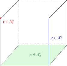
Let for denote the set of -dimensional generalised edges of . For example, if , are the vertices, the edges, and the faces; see Figure 3.1.
-
•
Let be the set of generalised edges of .
-
•
Let , the generalised edges of that are edges of .
-
•
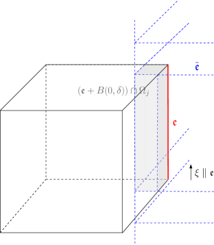
For and , we write (informally “ is parallel to ”) if , where , where are linearly independent vectors tangent to ; see Figure 3.2.
-
•
For , let if and otherwise.
-
•
For , , let
(informally, is the region a distance into the -dimensional edges of the PML layer of , taking into account that the PML layer is width for edges that are part of and otherwise ).
-
•
For , and , let
(3.1) where, for any , is a set of orthogonal outward-pointing (with respect to ) normal vectors to . Informally, is the region a distance into the part of the PML layer of corresponding to edge that is then extended out of to infinity, both normally (corresponding to in (3.1)) and tangentially (corresponding to in (3.1)); see Figure 3.2.
Let
-
•
For , let , i.e., the -strict PML layer of , and , i.e., the -strict extended PML layer of .
-
•
For , let , i.e., the -strict PML corners of , , i.e., the -strict extended PML corners of .
Additionally, when in the above notation we omit it; e.g., is written as and is written as .
3.2 Extensions of PML solutions in
Odd-symmetric extension on parts of that intersect .
Definition 3.1 (Odd-symmetric extension).
Let be such that there is a unique Euclidien coordinate system so that , where is open. For any , we denote its odd-symetric extension to , , defined by, for any
Let be a parameter to be fixed later. We define the extended domain
where, for any , is a set of orthogonal outward-pointing (with respect to ) normal vectors to ; i.e., is extended normally for a distance from the edges of that are (subset of) edges of . Note that if , then .
We now define an extension of functions from to by symmetrising multiple times with respect to the generalised edges of (and its partial extensions). The following definition is illustrated in Figure 3.3.
Definition 3.2 (Extension from to ).
For , we define the partial extension with respect to edges of dimension :
Observe in particular that and . For , define the extension from to in the following way. Let
where is defined piecewiese by Definition 3.1. When multiples choices of symmetrisation are possible, we chose one arbitrarily. We then set
We now fix small enough so that and does not vary normally in an -neighbourhood of (recall from §1.4 that we assume that in a neighbourhood of , each does not vary normally). As consequence of the latter,
| (3.2) |
Lemma 3.3 (Extension for homogeneous Dirichlet data).
Suppose , and are such that
Let and . If on , then and
| (3.3) |
Although we have so far been considering as an operator on , it is defined on all of by (1.3) and (1.4), and so its application in (3.3) on makes sense.
Proof of Lemma 3.3.
To prove that , the key calculation in 1-d is that
Since , . The result for is then proved in an analogous way.
Since , the extension only occurs when the PML scaling functions are either linear or zero. Therefore, by the definitions in §1.4.2, the coefficients of are constant near . The result (3.3) then follows from the definition of the weak derivative and integrating by parts. Indeed, in 1-d the basic calculation is that, for , if and for , then ; i.e. and so with . For , the calculation is more complicated, but the basic idea is the same, crucially using that the coefficients of are constant near . ∎
3.3 Semiclassical ellipticity statements for
We begin with a computation quantifying the ellipticity of at the symbolic level.
Lemma 3.4.
Let denote the semiclassical principal symbol associated with . Given a compact set , there exists such that for all and the following is true.
-
1.
(Bounding the symbol below by the PML scaling function)
-
2.
(Ellipticity at infinity in the variable)
Furthermore, the same properties hold for replaced with .
Proof.
Observe that
so that
| (3.4) |
On the one hand, the first equation in (3.4) implies that, for
from which Point 1 follows.
Since for with equality only when , given there exists and such that
Therefore, with ,
from which Point 2 follows. ∎
Recall from §B.2 that can be informally understood as . Similarly, can be informally understood as .
Lemma 3.5 (Directions of ellipticity).
(i.e., at a point in the extended PML layer of , the symbol vanishes only when is parallel to every extended generalised edge of that belongs to a -neighbourhood of).
4 A propagation result for the PML solutions and its consequences
The main purpose of this section is to prove the following propagation result (stated informally in §2.2, with the main ideas behind the proof described in §2.3).
Lemma 4.1.
The interpretation of Lemma 4.1 is that, in the “measurement location” of , the wavefront set of the (extended) solution consists at most of points coming from the wavefront set of the (extended) source under the forward flow; see Figure 4.2. The assumption in Point 1 is a non-trapping assumption.
Lemma 4.1 is proved in §4.3 below, with §4.1 and §4.2 containing intermediate results. §4.4 and §4.5 contain other consequences of the propagation results of this section, namely Lemma 4.5 (a priori bound on the PML solution operator) and Theorem 4.6 (error incurred by Cartesian PML approximation of outgoing Helmholtz solutions), respectively.
4.1 Forward propagation of regularity
Recall that is the Hamilton flow for defined by (1.15). Let denote the Hamilton flow for , that is, defined by (1.15) with replaced by . For any , let denote the Hamilton flow for , that is, defined by (1.15) with replaced by . Finally, given an interval , let
| (4.1) |
Lemma 4.2.
On , for any ; and on , for any .
Proof.
The following lemma uses the notion of wavefront set defined in Definition B.6 below.
Lemma 4.3 (Forward propagation of regularity from an elliptic point).
Let be a family of -tempered distributions in the sense of Definition B.5. Assume there exists , , and such that
| (4.4) |
Then . The same property holds with replaced with .
Proof.
We do the proof for , the proof for is similar. The objects involved in the proof are illustrated in Figure 4.1. We can assume that , otherwise the result follows directly from Lemma B.9.
The idea of the proof is the following: we seek to use forward propagation of regularity given by Lemma B.11. By the second assumption in (4.4), the trajectory under the flow (illustrated in red in Figure 4.1) doesn’t intersect until at least . However, to use Lemma B.11, we need that the trajectory under the flow doesn’t intersect , and this flow is not necessarily equal to once . A solution to this issue is the following. When travelling backwards from under (which starts off equal to by Lemma 4.2 and the fact that ), by continuity, the two flows must be close to each other in a short time interval after stops being zero, and in this time interval. That is, we know that under the backward flow, reaches an elliptic point of without hitting the data, and the result then follows from Lemma B.11.
In more detail: by Lemma 4.2,
(since the two flows are the same when ). By assumption (i.e., the existence of ), . By Lemma 4.2,
| (4.5) |
(where is defined analogously to (4.1) with replaced by ). By the definition of , there exists such that
| (4.6) |
By (4.5) and the second assumption in (4.4), since and is a closed set,
Hence, since is continuous, there exists close enough to so that
| (4.7) |
In particular, (4.6) and (4.7) imply by Lemma B.9 that
| (4.8) |
Forward propagation of regularity given by Lemma B.11 (the sign condition on being satisfied thanks to the first equation in (3.4)) allows us to conclude, by (4.8) and (4.7), that . ∎
4.2 Escape to ellipticity
Lemma 4.4 (Escape to ellipticity).
For any such that the backward trajectory from in the flow goes to infinity (i.e. is not trapped backward in time), there exists such that
Although Lemma 4.4 is stated (and then used below) with the flow associated to , we note that the result holds for a general continuous flow.
Proof of Lemma 4.4.
By Lemma 3.5, it suffices to show the existence of such that
For simplicity we give the proof in dimension 3; we then indicate how to generalise it to any dimension.
By the non-trapping assumption, there exists such that the backward trajectory from enters forever after time ; i.e., . Reducing if necessary, we have .
Observe that the trajectory from is in an extended PML-face for all times before time , i.e. for some . If there exists such that and , then we are done. Otherwise, the backward trajectory from stays parallel to the face it entered before leaving , and therefore there exists such that it enters an extended PML-edge forever; i.e., for some . Reducing if necessary, we have again .
If there exists such that and , then we are done. Otherwise, the backward trajectory from stays parallel to the edge it entered before leaving , and therefore there is with such that it enters a perpendicular PML-edge (because is a hyperrectangle). We therefore have and for some and we are done.
The proof generalises to any dimension by observing that, if and for some with , then either there exists such that and , or the corresponding trajectory enters a dimensional edge forever: i.e., there exists such that and with . The initialisation of this process (entering ) and the end-case () are the same as in dimension . ∎
4.3 Proof of Lemma 4.1
By the assumption in Point 2 and Lemma 3.3,
Let be such that
in other words, the backwards trajectory for the Hamilton flow of starting at either doesn’t intersect for any or leaves before intersecting such a subset. By Lemma 4.4, there exists such that
| (4.9) |
(where we take if ). From the first part of (4.9), by assumption on , we get that for any
| (4.10) |
We conclude from (4.9) and (4.10), by forward propagation of regularity from an elliptic point, given by Lemma 4.3, that .
4.4 A priori bound on the local PML solution on the subdomains
Lemma 4.5 (Bound on PML solution operator).
Assume that the flow associated with is nontrapping. There exists and such that the following is true. Given and , if satisfies
| (4.11) |
then if then
| (4.12) |
The same holds with replaced with .
We emphasise that the in front of the norm of on the right-hand side of (4.12) is not sharp. However, the only way in which (4.12) is used in the proofs of Theorems 1.1-1.6 is to show that the solution to (4.11) is tempered (in the sense of Definition B.5) if and are tempered, and so this non-sharpness is not important for the results of the paper.
Proof.
We first claim that it it sufficient to prove that there exists , such that if satisfies then, if ,
| (4.13) |
Indeed, by [43, Theorem 5.6.4], for any Lipschitz domain there exists such that for all , where is the trace operator. Furthermore,
| (4.14) |
noting that the weighted norm on used in [43] is equivalent to and the weighted norm on used in [43] is equivalent to . Therefore, with the solution to (4.11), let . Then, by (4.13),
We now prove the bound (4.13). Seeking a contradiction, we assume that (4.13) does not hold. Then, there exists , , , such that and
Renormalising, we can assume that
| (4.15) |
Then
| (4.16) |
We now extend and to using the extension defined by Lemma 3.2; i.e., we let and . By Lemma 3.3, . By (4.15) is tempered, and so propagation of singularities applies. For any , by (3.3) and the fact that (by Lemma 3.3),
Therefore, by (4.16) and the definition of (Definition B.6),
| (4.17) |
By Lemma 4.4 (escape to ellipticity), Lemma 4.3 (forward propagation of regularity from an elliptic point), and (4.17),
Therefore, by Lemma B.8, Point 1 together with Point 2 of Lemma 3.4 (ellipticity at infinity) and (4.16),
Lemma B.8, Point 2 together with Point 2 of Lemma 3.4 and (4.16) allow us to strengthen this to
which contradicts (4.15). ∎
4.5 Error incurred by Cartesian PML approximation of outgoing Helmholtz solutions
Theorem 4.6.
(The error in Cartesian PML approximation of outgoing Helmholtz solutions .) Suppose either (i) is nontrapping, or (ii) with considered as an operator either or , its solution operator is bounded polynomially in . Then for any , there exists such that the following holds for all . Let and let and be the solutions to
Then,
Theorem 4.6 is not used in the proofs of Theorems 1.1-1.6, but we include it in the paper because of its independent interest. Indeed, as noted in §1.2, the only other -explicit Cartesian-PML convergence result in the literature is that of [10, Lemma 3.4] for the case (i.e., no scatterer), with this proof based on the explicit expression for the Helmholtz fundamental solution in this case. -explicit convergence results for radial PMLs applied to general Helmholtz problems are in [20].
Proof.
By dividing and by , we can assume, without loss of generality, that . It is then sufficient to prove that
Let be the solution to
By [14, Theorem 4.37],
| (4.18) |
indeed, the Cartesian PML fits into the framework of [14, §4.5.1] by setting
and observing that and in the sense of quadratic forms (i.e., is convex) since . The relation (4.18) implies that it is sufficient to prove that
| (4.19) |
We claim that
| (4.20) |
and postpone the proof for now.
We now let be the solution to
By (4.20) and either Lemma 4.5 under Assumption (i), or polynomial boundedness of the solution operator on under Assumption (ii),
| (4.21) |
By Lemma B.8, Part 2, the bound (4.21) can be improved to
| (4.22) |
The whole point of the definition of is that, by uniqueness of ,
Thus (4.19), and hence also the result, follows from (4.22).
We now prove (4.20). Under Assumption (ii), is immediately tempered in the sense of Definition B.5. Under Assumption (i), repeating the proof of Lemma 4.5 (without the extensions), we see that is polynomially bounded in in terms of the data for any , and hence is tempered.
Let be such that near and . We now seek to apply Lemma 4.1. By Lemma 3.5, any is perpendicular to the scaling direction. Therefore, since in the PML region, any such goes to infinity backwards in time under the flow associated to . Therefore Point 1 in Lemma 4.1 is satisfied, and the result of this lemma is that
By similar arguments, Lemma 3.5 implies that
By Lemma B.9,
By Lemma B.8, Part 1, and Lemma 3.4, Part 2, for any ,
(where Lemma B.8 is applied with , so that ). The claim (4.20) then follows from the trace theorem and the fact that near , and the proof is complete. ∎
5 The propagation of physical error
5.1 The propagation of physical error for the parallel method
Proof of Lemma 2.1.
By the definition of (2.4), on for any . Thus, since (by (1.6)), on and so defined by (2.5) maps . Now, in , by the definition of (2.1) and the iteration (1.7),
Therefore, by (2.2),
Furthermore, by (1.7), on , and thus, on ,
Therefore, by the definition of (2.4), and the fact (noted after (2.3)) that ,
Therefore, since ,
Remark 5.1 (The rationale for putting in the definition of ).
The end of the proof of Lemma 2.1 shows that if is omitted from the definition of , then the result (2.6) still holds. The advantage of including is that this builds into the operator the localisation property of the physical error. Indeed, we do not expect the power contractivity proved for (which is a result about applied to arbitrary functions in ) to hold if is omitted from the definition of .
5.2 The propagation of physical error for the sequential method
Proof of Lemma 2.7.
We prove the first equation in (2.16); the proof of the second equation is very similar. To keep the notation concise, in the proof we omit the restrictions onto so that, in particular, the PDE defining in (1.10) becomes
By the definition of (2.13) and the definition of (1.10), in ,
Similarly, on ,
where, in the last equality, we used the same manipulation as in the previous displayed equation. Therefore, by definition of (2.4) and the definition of in §2.1,
Therefore
The result (i.e., the first equation in (2.16)) follows by the definition of (2.5) and the fact that and are the lower/upper triangular parts of . ∎
The following lemma is proved in an analogous way to Lemma 2.7.
Lemma 5.2.
For the general sequential method with ordering , for ,
where
Comparing Lemmas 2.7 and 5.2, we see that, for the forward-backward method, both and alternate between equalling and .
By their definitions, we see that is non-zero if appears before in the ordering of subdomains and is non-zero if appears after in this ordering. Compare this to the fact that is non-zero if , i.e., appears before in the ordering or after in the ordering , and is non-zero if , i.e., appears after in the ordering or before in the ordering .
6 Proof of Theorem 1.6
6.1 Precise definition of following a word
Recall from §2.2 the definitions of the set of words and the composite map (2.9). Recall the definition of the trajectory staring at for a time interval , (4.1).
We now define a set of cutoffs that are bigger than the s. Let be such that, for each , , , on , and is zero on .
Definition 6.1.
A trajectory for follows a word of length if
where the product stands for concatenation, for some and with
-
•
for , ,
-
•
for (recall Definition 3.2 of the extended domains),
-
•
.
Figure 2.2 illustrates a simple example of a trajectory following a word.
6.2 Reduction to a propagation result for (Lemma 6.2)
Recall that in §2 we showed how Theorem 1.6 follows from Lemma 2.4; i.e., the result that
The heart of the proof of Lemma 2.4 is the following result, described informally in §2.2, and proved in the next subsection using the propagation result of Lemma 4.1.
Lemma 6.2.
Suppose that is nontrapping. Let of length . For any and any tempered -family of elements of , is tempered and
| (6.1) |
where .
Proof of Lemma 2.4 using Lemma 6.2.
The fact that is tempered is a consequence of the resolvent estimate given by Lemma 4.5. We fix a word not allowed. Seeking a contradiction, we assume that (2.10) fails; that is, there exists , with and such that
We show that
leading to a contradiction. To lighten the notation, from now on we drop the subscripts from and . By the definition of a word being allowed, Lemma 6.2 implies that, for any ,
Therefore, by Lemma B.8, Part 1 together with Lemma 3.4, Part 2,
| (6.2) |
Recall that has a at the front by the definitions of (2.9) and (2.5). We now choose in (6.2) to be one on and supported in , and obtain that
∎
Remark 6.3 (Why we don’t extend interior subdomains).
Consider the end of the proof of Lemma 2.4 using Lemma 6.2. If is an interior subdomain, i.e., , then is compactly supported in (indeed, its support does not touch the PML layer of ), and we can choose to be compactly supported in ; i.e., we do not need information about up to . However, if is not an interior subdomain, then can be supported up to the boundary of (by the partition of unity property) and we therefore need information about up to . This is why we extend to , choose to have support in , and do the propagation in the interior of (to bypass the issue of propagating up to , as discussed in Remark 2.5).
6.3 Proof of Lemma 6.2 (ending the proof of Theorem 1.6)
It therefore remains to prove Lemma 6.2. The idea of the proof is to iteratively apply Lemma 4.1. We proceed by induction on the length of . We first assume that the result of the lemma holds for any word of length and we show it for any word of length . At the end of the proof we show that the result holds when .
If , we decompose as
and write (by the definitions of (2.9) and (2.4))
We now apply Lemma 4.1. Let
so that . By (3.2),
| (6.3) |
By the definition of (2.4),
where we omit the restriction operators on to keep the notation concise (as in the proof of Lemma 2.7 above).
We therefore apply Lemma 4.1 with , , , and .
We need to check that the assumptions in Points 1-2 are satisfied. The assumption in Point 1 is satisfied because is nontrapping. The assumption in Point 2 is satisfied since by Lemma 2.1.
The result of Lemma 4.1 is that
where , . Recall that in the extended region the PML is linear and the coefficients of both and are constant. The arguments used in the proof of Lemma 3.3 therefore show that the extension operator of Definition 3.2 is such that
| (6.4) |
where we have used (3.2) in the second step.
Therefore
| (6.5) |
We ultimately use that, by (B.4) and (B.5),
| (6.6) |
where is such that on . However, we first change the cut-off into a cut off in so that we can use the induction hypothesis, which gives information about with .
Observe that
(note that this crucially relies on the presence of on the right of both sides of the equality).
Using this in (6.5), we have
| (6.7) |
Therefore, by (6.6) with replaced by ,
Therefore, by the induction hypothesis that (6.1) holds with replaced by and then the Definition 6.1 of following a word,
and the result for words of length , assuming the result for words of length , follows by (6.3). To complete the induction, we prove the result for words of length . If , then the inclusion (6.7) simplifies to
Arguing as in (6.6) and using the definition of following a word (Definition 6.1), we obtain
and the proof is complete.
7 Proofs of Theorems 1.1, 1.2, 1.3, 1.4
7.1 Checkerboard coordinates
For concreteness we use the natural coordinates coming from the checkerboard construction in §1.4.7. For a -checkerboard, the coordinates (with origin ) of the subdomain are where if the from which is formed equals .
For a -checkerboard, we omit the directions that have to obtain coordinates .
7.2 Allowed words in a checkerboard when
Lemma 7.1.
Assume that is a checkerboard and . Then, if is allowed, for any , the map is monotonic.
Proof.
The underlying idea of the proof is that a straight line through a non-overlapping checkerboard (i.e., the decomposition of described in Point (i) of §1.4.7) necessarily has monotonic coordinate maps. The subtlety here is that the subdomains overlap; however, the fact that an allowed word must pass through the (disjoint) subdomains in (2.7) essentially puts us back in the non-overlapping case.
Assume that , otherwise the statement is void. By the definition of allowed, there exists a trajectory following . Since the coefficients are constant, this trajectory is a straight line, and by the definitions of allowed (Definition 2.2) and follow (Definition 6.1), the trajectory intersects
Since is supported in and away from , this implies that for and for . It follows that there exists on a line with , and . Because and is a checkerboard, it follows that for any such that , if and only if (where subscript denotes the th coordinate of in ); note that for this to be true it is key that the is not in the overlap of and (which we have ensured above). The result follows. ∎
7.3 Proofs of Theorems 1.1 and 1.3 (i.e., the results about the parallel method with )
7.4 Exhaustive sequence of orderings
Given a sequence of orderings , for every we define the order relation on by
i.e., if at step of the method, comes before .
Recall that is a fixed set of checkerboard coordinates, i.e., is such that is the th coordinate of on the checkerboard.
Definition 7.2 (Exhaustive ordering).
We say that an ordering is exhaustive if (i) for any , there is such that , and (ii) for any sequence of elements of such that
| (7.1) |
there exists an so that
| (7.2) |
Recall the informal definition of exhaustive in §1.6 that (i) given any ordering in the sequence, the sequence also contains the reverse ordering (i.e., where the subdomains are visited in reverse order), and (ii) given any directed straight line (here a sequence of subdomains with monotonic coordinate maps (7.1)) the sequence of sweeps has to contain at least one sweep such that the subdomains in the straight line are visited in order, but not necessarily sequentially, in that sweep; i.e., (7.2).
Observe that, if are the indices of reverse orderings, as in Definition 7.2, then .
In what follows, we assume that the Cartesian directions on the checkerboard are always ordered in the same way, i.e., if and are two set of checkerboard coordinates, then and represent coordinates in the same th direction.
Example 7.3 (Lexicographic orderings).
Let be the vertices of the checkerboard. For , let be the set of checkerboard coordinates with as origin. Define , for , to be the lexicographic order with respect to , ie the lexicographic order with vertex as origin. Then is exhaustive. One such ordering is given by defining
this is shown in the case and in Figure 1.2.
Example 7.4 (An algorithm for generating exhaustive sequences of orderings).
Let
be the vertices of the checkerboard.
For any ,
let be
the set
of checkerboard coordinates with as origin. For ,
if is not already defined, define in such a way that all the maps are non-decreasing,
then, for such that has for coordinates , define . Then is exhaustive.
Figure 7.1 illustrates an exhaustive sequence of orderings for a 33 checkerboard following the algorithm in Example 7.4.
| 6 | 8 | 9 |
|---|---|---|
| 4 | 5 | 7 |
| 1 | 2 | 3 |
| 4 | 2 | 1 |
|---|---|---|
| 6 | 5 | 3 |
| 9 | 8 | 7 |
| 9 | 6 | 5 |
|---|---|---|
| 8 | 4 | 2 |
| 7 | 3 | 1 |
| 1 | 4 | 5 |
|---|---|---|
| 2 | 6 | 8 |
| 3 | 7 | 9 |
Lemma 7.5.
On a -checkerboard, if is exhaustive then .
Proof.
Suppose we have an exhaustive sequence of orderings on a -checkerboard. Label the subdomains
By the definition of exhaustive, there exist an ordering that visits (in order) and an ordering that visits (in order) , with these subdomain orderings corresponding to diagonal lines from the top left to bottom right passing, respectively, below and above the centre.
If , then equals either or . In either case, neither ordering, nor its reverse, visits or in order (with these subdomain orderings corresponding to diagonal lines from the bottom left to top right passing, respectively, below and above the centre). Therefore the sequence of orderings consisting of and its reverse is not exhaustive, and so .
If then the reverse ordering to (which visits in order, and hence before ) is neither (which visits in order, and hence after ) or the reverse ordering to (since ). Therefore .
For an arbitrary 2-checkerboard, we repeat the argument above in the top left corner. ∎
7.5 Proof of Theorem 1.4
Arguing as in the proof of Theorem 1.2 outlined in §2.5, and using Lemma 5.2 instead of Lemma 2.7, we obtain
where we used that since is the rearrangment of an lower-triangular matrix. It follows that
and Theorem 1.4 therefore follows immediately from the following lemma.
Lemma 7.6.
Assume that is exhaustive (in the sense of Definition 7.2). Then, for any ,
To prove Lemma 7.6, we identify the words arising in the entries of the products , show that they are not allowed, and then apply Lemma 2.4.
Lemma 7.7.
Assume that is exhaustive. Then, no word satisfying
| (7.3) |
where is a surjective sequence with values in is allowed.
Proof of Lemma 7.6 assuming Lemma 7.7.
Let
Observe that
| (7.4) |
and
| (7.5) |
Now, any product of and , , can be understood as the sum of for suitable words . Recall from the definition of (2.9) that the last letter in appears in the left-most operator in the composition defining . The equation (7.4) therefore implies that left-multiplying such a product by results in a linear combination of operators such that the last letter of (corresponding to in (7.4)) is the previous letter (corresponding to in (7.4)). Similarly, (7.5) implies that left-multiplying a product of and , , by results in a linear combination of operators such that the last letter of (corresponding to in (7.5)) is the previous letter (corresponding to in (7.5)).
By induction, it follows that the entries of are linear combinations of operators of the form , where is a word of size that can be written as the concatenation
where
and each word for is of size and verifies
Observe that, by definition of , for any
On the other hand, by the definition of exhaustive, for any , there is such that . We thus have, for any
It follows that, denoting , there is a surjective sequence with values in so that
Hence is not allowed by Lemma 7.7, and Lemma 2.4 gives the result. ∎
Proof of Lemma 7.7.
Seeking a contradiction, assume that such a word is allowed. By Lemma 7.1, all the coordinates maps are monotonic. As a consequence, since is exhaustive, there exists an so that
| (7.6) |
However, there exists such that . Therefore, by the assumption (7.3) and (7.6)
hence , which contradicts the definition of a word. ∎
Remark 7.8 (The analogue of Theorem 1.4 when ).
In the general case when , we define an ordering to be exhaustive if (i) for any , there is such that , and (ii) for any allowed word of size , there exists an so that
The proofs of Lemma 7.6 and Lemma 7.7 still hold, and this therefore leads immediately to the generalisation of Theorem 1.4 when with the result that, if is exhaustive (as defined above) and of size then
For such orderings to always exist, one would need in principle to define the sequential method in a more general way by not imposing the to be bijections, allowing to visit a subdomain multiple times during a single sweep – as would a non-straight trajectory visiting the same subdomain multiple times. Constructing such orderings is, however, difficult, since it depends on the specific dynamic of the Hamilton flow imposed by the non-constant , and we have therefore not pursued this further in this paper.
8 Numerical experiments
8.1 The overlapping Schwarz methods on the discrete level
Given a finite-dimensional subspace of , which we denote by , the discrete analogues of the parallel and sequential methods described in §1.4.5 and §1.4.6 (respectively) compute approximations to the solution of (1.5) in using Galerkin approximations to the solutions of the local problems (1.7) and (1.13) in appropriate subsets of .
We now describe this process in detail for the discretisation of the parallel overlapping method in §1.4.5, showing that it gives a natural PML-variant of the well-known RAS (restricted additive Schwarz) method (introduced in [8]).
The Galerkin approximation of the PDE (1.5).
Let be a shape-regular conforming sequence of meshes for . We assume that the edges of resolve the boundaries of , , , and , for all ; since all these domains are unions of hyperrectangles, this is straightforward to achieve in practice.
Let be the standard finite-element space of continuous piecewise-polynomial functions of degree on . Given , the Galerkin approximation to the solution of (1.5) is defined as the solution of the problem: find such that
| (8.1) |
where the sesquilinear form is obtained by multiplying the PDE (1.5) by a test function and integrating by parts; i.e., when ,
| (8.2) |
where
with and .
The Galerkin approximations of the local problems.
Let be the sesquilinear form obtained by multiplying be a test function and integrating by parts; when the definition of is the same as the definition of (8.2) except that , is replaced by .
Let and let be the operator associated with ; i.e.,
| (8.4) |
We assume that that all the operators and are invertible. When the Helmholtz problem on is nontrapping, we expect this to be true when is sufficiently small; this threshold was famously identified for the 1-d Helmholtz -FEM in [29], and the latest results for proving existence of the Galerkin solution (along with error bounds) under this threshold are given in [21]. The results of [21], however, are not immediately applicable when is a hyperrectangle because of the low regularity of .
Restriction and prolongation operators.
We define the prolongation operator by, for ,
Let be the adjoint of , i.e.,
| (8.5) |
We also define a weighted prolongation operator , involving the partition-of-unity function , by
where is nodal interpolation onto . Then, for all and all finite element nodes ,
i.e.,
| (8.6) |
The discrete parallel overlapping Schwarz method.
Let be the finite-element approximation to the local corrector (1.9); i.e., given , is the solution of
Thus, by (8.3), (8.4), and (8.5),
In analogy with the second equation in (1.9) and recalling (8.6), we then define
i.e., the method is the preconditioned Richardson iteration
| (8.7) |
The preconditioner is of the form of the RAS preconditioner [8], with the crucial fact that it involves the weighted prolongation operator instead of (compare, e.g., [12, Definitions 1.12 and 1.13]). The classical ‘Optimised’ RAS (known as ORAS [50], [12, §2.3.2]) for Helmholtz uses the impedance boundary condition on the subdomain boundaries (see, e.g., [26, 27]), but here we have PML at the subdomain boundaries. We note that numerical results on this version of RAS when the PML scaling function is proportional to were given in [4].
GMRES.
The main results of the paper concern the overlapping Schwarz methods described in §1.4.5 and §1.4.6 as fixed-point iterations (on the continuous level). We also present numerical results for the generalised minimal residual (GMRES) algorithm [48] acting as an acceleration of the parallel fixed point iteration in (8.7). Since the iteration counts of the sequential method used as a fixed-point iteration are relatively low, we do not consider GMRES acceleration for this iteration here.
We therefore briefly recall the definition of GMRES applied to the abstract linear system where is an nonsingular complex matrix. For GMRES applied to the parallel method above, is the matrix corresponding to the operator and is the vector corresponding to . Given initial guess , let and
For , define to be the unique element of satisfying the minimal residual property:
8.2 Common set-up for the experiments
The Helmholtz problem.
We work in with and PML width , so that . Note that, for , the number of wavelengths in the PML is , respectively. We take the PML scaling function as , and the right-hand side of the PDE (1.5) to be when . Note that taking the right-hand side to be a Helmholtz solution, similar to for a scattering problem, ensures that all of the mass of the solution in phase space is oscillating at frequency approximately , ensuring that the solution propagates.
The domain decomposition.
We consider both strip and checkerboard decompositions of . The overlapping decomposition (1.2) is taken to have overlap , with then each overlapping subdomain extended by PML layers of width .
The smooth partition of unity functions are constructed with respect to a (still overlapping) cover of consisting of subsets of , so that each POU function vanishes in a neighbourhood of . In more detail, for strip decompositions with , we let
and
The PoU functions are then defined by For checkerboard decompositions, the PoU functions are created by normalising the Cartesian product of .
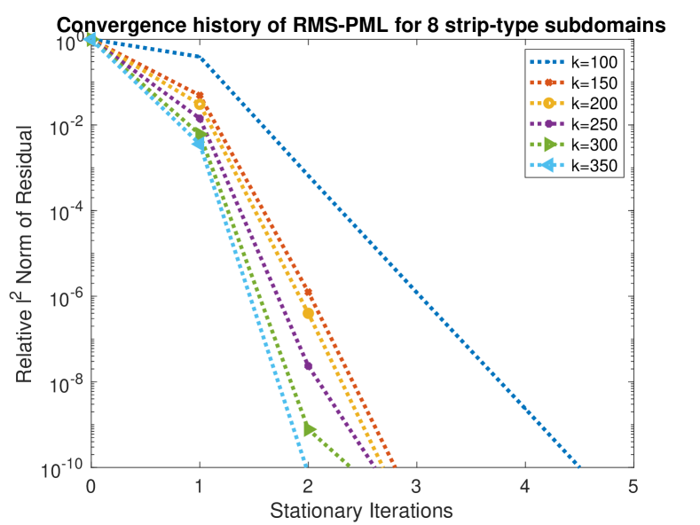
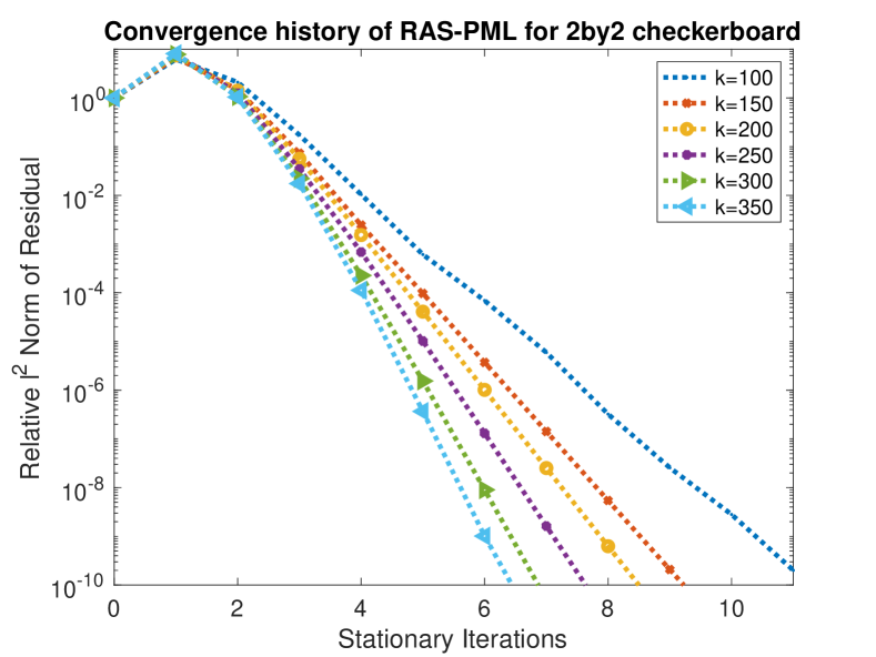
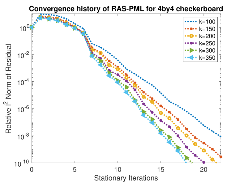
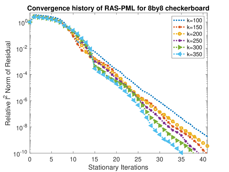
We use the abbreviations RAS-PML and RMS-PML to denote the parallel (additive) and sequential (multiplicative) methods, respectively.
The finite-element method.
The finite-dimensional subspace is taken to be standard Lagrange finite elements of degree on uniform meshes of , with chosen as the largest number such that is an integer (recall from the discussion immediately below (8.4) that we expect the relative-error of the finite-element solutions to be bounded uniformly in under this choice of ). We write the resulting linear system as
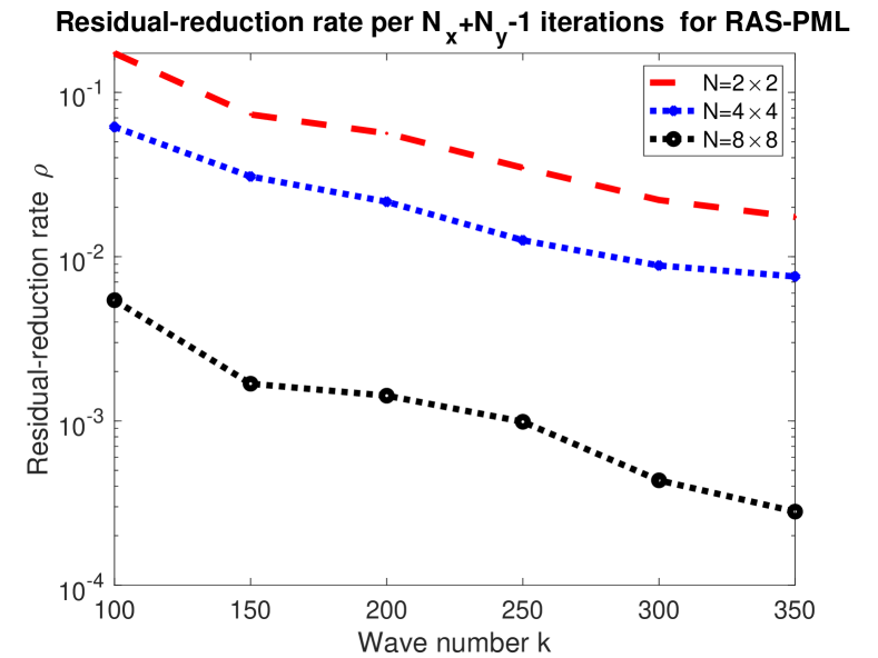
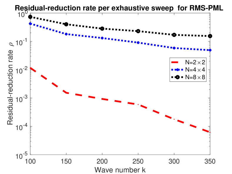
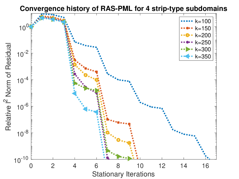
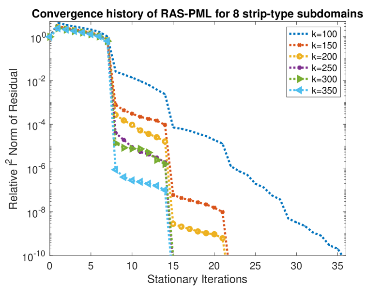
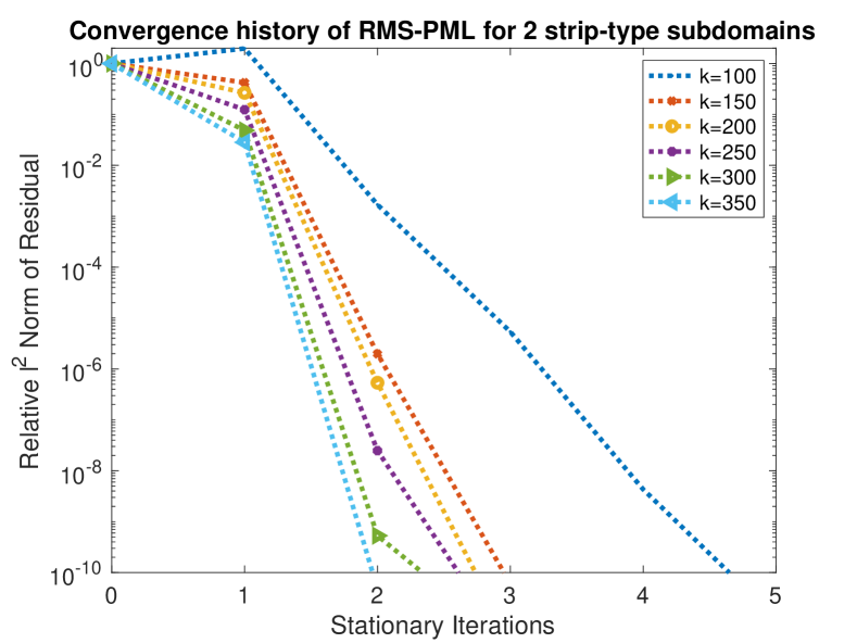
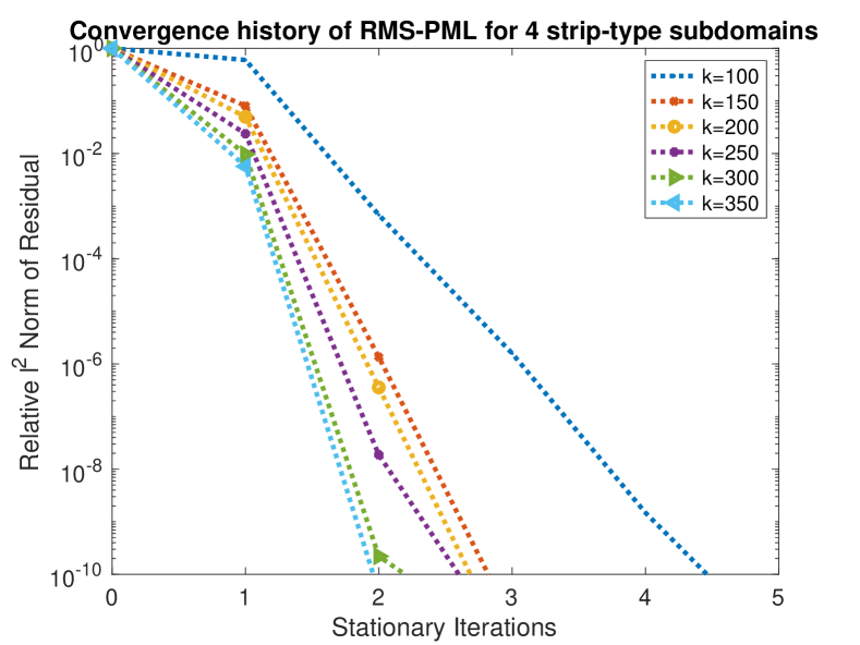
8.3 Experiment I:
Figure 8.1 plots the rate that the residual decreases as a function of for
-
•
a strip decomposition, with RAS-PML (Plot (a) of the figure) and RMS-PML with forward-backward sweeping (Plot (b)),
-
•
a checkerboard decomposition, with RAS-PML (Plot (c)) and RMS-PML with the exhaustive sequence of four orderings constructed via Example 7.3 (Plot (d)).
In all cases the rate of residual reduction increases as increases (as expected from Theorems 1.1-1.4 and 1.6).
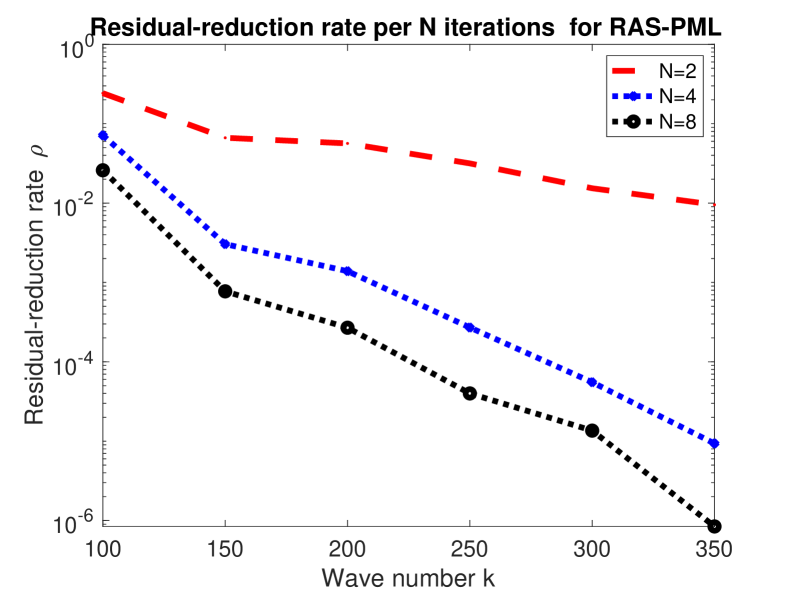
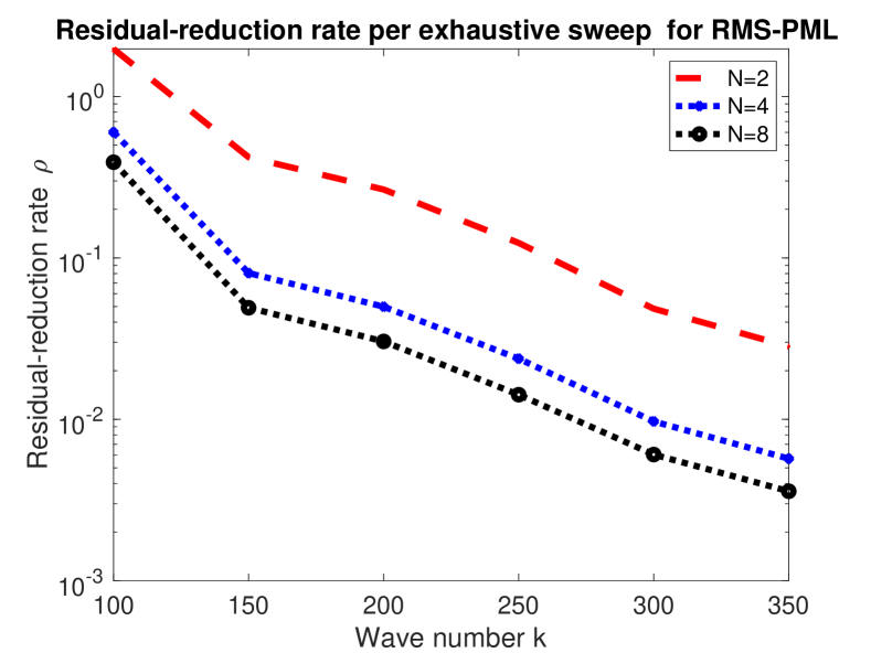
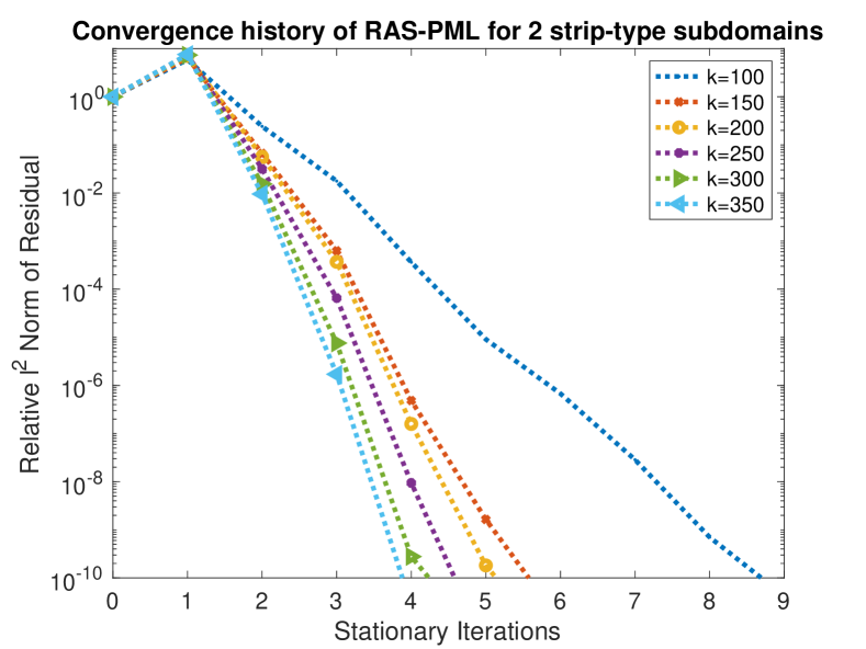
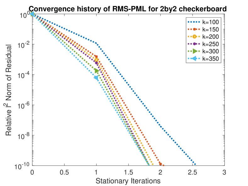
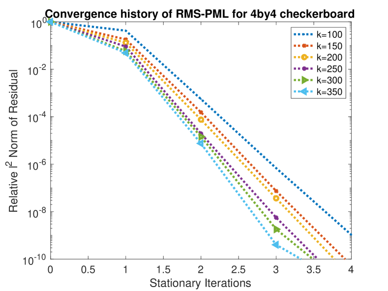
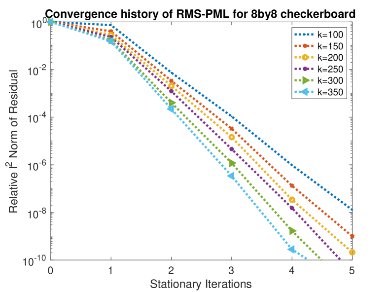
Figures 8.2, 8.3, 8.4, and 8.5 present the convergence histories for RAS-PML and RMS-PML for different s and different domain decompositions. We highlight that, for the strip decompositions with and , Figure 8.2 shows that the residual for RAS-PML on a strip undergoes a significant reduction after every iterations, as expected from Theorem 1.1.
8.4 Experiment II: variable
We consider three cases
-
Case 1:
,
-
Case 2:
decreases linearly from the center to and equals 1 for
-
Case 3:
increases linearly from the center to and equals 1 for
When decreases, i.e., increases, as a function of , then the problem is nontrapping (see, e.g., [28, Theorem 2.5], [28, §7]). If increases quickly enough as a function of , then the problem is trapping [44], but the growth of the solution operator through an increasing sequence of s is very sensitive to the particular value of [32], and depends on the data [11]. Therefore, in these experiments, we do not seek to solve any trapping problems where the solution operator grows faster with than for nontrapping problems.
Experiment I showed that, in Case 1 (), the rate of residual reduction increases with for all the methods considered. In this experiment, we compare Cases 1-3 by listing the fixed-point iteration counts (in brackets, GMRES iterations) to obtain the following relative-residual reduction
| (8.8) |
with Table 1 considering RAS-PML on strips, Table 2 considering RMS-PML on strips, Table 3 considering RAS-PML on checkerboards, and Table 4 considering RMS-PML on checkerboards. In all scenarios the number of iterations are very similar for each of Cases 1, 2, and 3.
| Variable | Case 1 | Case 2 | Case 3 | ||||||
|---|---|---|---|---|---|---|---|---|---|
| \ | 2 | 4 | 8 | 2 | 4 | 8 | |||
| 100 | 6(6) | 11(11) | 23(22) | 6(6) | 13(12) | 26(23) | 7(6) | 11(10) | 22(22) |
| 150 | 4(4) | 7(7) | 15(15) | 5(4) | 10(10) | 18(18) | 5(4) | 10(8) | 17(15) |
| 200 | 4(4) | 7(7) | 15(15) | 4(4) | 10(10) | 18(15) | 4(4) | 10(8) | 15(15) |
| 250 | 4(4) | 7(7) | 15(15) | 4(4) | 10(8) | 18(15) | 4(4) | 8(7) | 14(14) |
| 300 | 4(4) | 7(7) | 15(15) | 4(4) | 10(8) | 15(15) | 4(4) | 8(7) | 15(15) |
| 350 | 4(4) | 5(5) | 8(8) | 4(4) | 10(7) | 13(13) | 4(4) | 7(7) | 13(13) |
| Variable | Case 1 | Case 2 | Case 3 | ||||||
|---|---|---|---|---|---|---|---|---|---|
| \ | 2 | 4 | 8 | 2 | 4 | 8 | |||
| 100 | 4 | 4 | 4 | 4 | 3 | 3 | 4 | 4 | 4 |
| 150 | 3 | 3 | 3 | 3 | 3 | 3 | 3 | 3 | 3 |
| 200 | 2 | 2 | 2 | 3 | 3 | 2 | 3 | 2 | 3 |
| 250 | 2 | 2 | 2 | 2 | 2 | 2 | 2 | 2 | 2 |
| 300 | 2 | 2 | 2 | 2 | 2 | 2 | 2 | 2 | 2 |
| 350 | 2 | 2 | 2 | 2 | 2 | 2 | 2 | 2 | 2 |
| Variable | Case 1 | Case 2 | Case 3 | ||||||
|---|---|---|---|---|---|---|---|---|---|
| \ | |||||||||
| 100 | 8(7) | 18(16) | 30(27) | 8(7) | 20(18) | 34(30) | 8(7) | 17(15) | 28(27) |
| 150 | 7(6) | 16(15) | 28(25) | 7(6) | 17(16) | 30(27) | 7(6) | 15(14) | 27(24) |
| 200 | 7(6) | 15(14) | 27(25) | 7(6) | 16(15) | 29(26) | 7(6) | 14(14) | 25(24) |
| 250 | 6(5) | 14(13) | 26(24) | 6(6) | 15(14) | 28(26) | 7(6) | 13(13) | 25(23) |
| 300 | 6(5) | 13(13) | 26(23) | 6(6) | 15(14) | 26(25) | 6(6) | 13(12) | 25(22) |
| 350 | 6(5) | 13(12) | 25(23) | 6(6) | 15(14) | 25(24) | 6(6) | 12(12) | 23(21) |
| Variable | Case 1 | Case 2 | Case 3 | ||||||
|---|---|---|---|---|---|---|---|---|---|
| \ | |||||||||
| 100 | 2 | 3 | 4 | 2 | 4 | 5 | 2 | 3 | 4 |
| 150 | 2 | 3 | 4 | 2 | 3 | 4 | 2 | 3 | 4 |
| 200 | 2 | 3 | 4 | 2 | 3 | 4 | 2 | 3 | 4 |
| 250 | 2 | 3 | 4 | 2 | 3 | 4 | 2 | 3 | 4 |
| 300 | 2 | 3 | 4 | 2 | 3 | 3 | 2 | 3 | 3 |
| 350 | 2 | 3 | 3 | 2 | 3 | 3 | 2 | 3 | 3 |
8.5 Experiment III: variable coefficient in the differential operator
Remark 2.6 above described how the results in Theorems 1.1-1.4 and 1.6 do not hold for the problem
| (8.9) |
where
and is a general symmetric-positive-definite-matrix-valued function with . This experiment demonstrates that the parallel Schwarz method diverges when applied to (8.9), where the local problems involve the operator (2.12).
In common with the previous two experiments, is the unit square in 2-d, now centred at the origin to make the expressions for simpler. We let and
| (8.10) |
i.e., transitions from being equal to at the origin to being equal to near the start of the PML. The variational formulation of (8.9) is (8.1) with the sesquilinear form now
where
with and as before. The local sesquilinear forms are defined analogously, with , replaced by .
We consider a strip decomposition with two subdomains and overlap . We display the results for PML width . The number of wavelengths in the PML at are then and respectively.
Table 5 displays the number of fixed-point iterations (in brackets, GMRES iterations) required to achieve the residual reduction (8.8), both for the coefficient given by (8.10) and (for comparison) . Table 5 shows that the parallel Schwarz method applied to (8.9) with given by (8.10) converges when (with iteration counts almost identical to the case ), but diverges when and when .
When PML is used to approximate the radiation condition, the accuracy increases with the width of the PML (see [30, Theorem 5.5], [6, Theorem 5.7], [20, Theorems 1.2 and 1.5]). The fact the the behaviour of the parallel Schwarz method with gets worse as the PML width increases is consistent with the fact, highlighted in Remark 2.6, that PML is not intended to be used when (in the sense that the imaginary part of the principal symbol is not single-signed).
| given by (8.10) | ||||||
|---|---|---|---|---|---|---|
| \ | ||||||
| 100 | 7(7) | diverges(14) | diverges(24) | 6(6) | 4(4) | 7(7) |
| 150 | 5(5) | diverges() | diverges() | 4(4) | 3(3) | 5(5) |
| 200 | 5(5) | diverges() | diverges() | 4(4) | 3(3) | 4(4) |
| 250 | 4(5) | diverges() | diverges() | 4(4) | 3(3) | 3(3) |
| 300 | 4(5) | diverges() | diverges() | 4(4) | 3(3) | 3(3) |
| 350 | 4(4) | diverges() | diverges() | 3(4) | 3(3) | 3(3) |
Appendix A Extending the main results to more general complex absorbing-layer operators
A careful examination of the assumptions used in the proof of Theorems 1.1-1.6 shows that these results hold under the following abstract assumptions, in which and ( standing for “absorbing”) play the role of (and generalise) and , respectively.
Theorem A.1.
Let be an overlapping decomposition of associated with the partition of unity . Let be second-order semiclassical pseudodifferential operators (in the sense of §B.2) with denoting their semiclassical principal symbols and denoting the Hamiltonian flows associated to , and respectively (i.e. defined by (1.15) with replaced by the appropriate symbol). Assume further that and satisfy the following.
-
1.
(Constant coefficients near ) and can be written near as second-order differential operators with constant coefficients and zero first-order coefficients.
-
2.
(Agreement of and ) on .
-
3.
(Ellipticity)
-
4.
(Respecting propagation)
-
(a)
On , for any ; and on , for any (cf. Lemma 4.2).
-
(b)
near , and near .
-
(a)
Then the results of Theorems 1.1, 1.2, 1.3, 1.4, 1.6 hold (replacing by in the definition of the iterates).
Proof of Theorem A.1.
As discussed in §2.4, the proofs of Theorems 1.1, 1.2, 1.3, 1.4, 1.6 are the consequences of
-
(i)
Algebra of the error propagation, showing which words appear in the products .
-
(ii)
Semiclassical analysis, showing that if is not allowed (Lemma 2.4).
-
(iii)
Properties of the trajectories of the flow associated with , dictating which are allowed.
By Point 2, the regions are unchanged, so that, in particular,
| (A.1) |
This implies that (i) above remains unchanged. We define both the notion of following a word and the quantity exactly as before (i.e., by Definition 6.1 and (2.8), respectively).
For (ii), we observe that the proof of Lemma 2.4 uses only the following properties of , and :
- •
-
•
Lemma 6.2 (a composite map follows the associated word).
The proof of Lemma 6.2 in turn uses only:
- •
-
•
the property (A.1), and
- •
The proofs of Lemma 4.5 and Lemma 4.1 use only the following: for both Lemma 4.5 and Lemma 4.1:
- •
- •
- •
∎
Theorem A.2.
(Approximation of outgoing Helmholtz solutions.) Assume that and satisfy the assumptions of Theorem A.1, and, in addition, that
-
1.
, with smooth and positive definite, smooth and strictly positive, and in a neighbourhood of .
-
2.
in .
-
3.
Either (i) is non-trapping, or (ii) the solution operators for and , as operators on, respectively, and , are bounded polynomially in .
Let , and let and satisfy
Then
Proof.
Recall from the proof of Theorem A.1 that, under the assumptions of Theorem A.1, Lemma 4.1 and Lemma 4.5 hold with replaced with .
By dividing and by , we can assume, without loss of generality, that . When Point 3.(ii) holds, both and are tempered directly by assumption. When Point 3.(i) holds, is tempered by the non-trapping solution-operator bound for (from [39] together with either [55, Theorem 3]/ [56, Chapter 10, Theorem 2] or [34], or [7, Theorem 1.3 and §3]) and is tempered by Lemma 4.5 (with replaced with ).
Let be such that near . Let
and observe that
Since satisfies the Sommerfeld radiation condition,
indeed, this is a classical consequence of Rellich’s uniqueness theorem, the outgoing properties of the free resolvent, and propagation of singularities; see e.g., [19, Proof of Lemma 3.4]. Therefore
Let ; we aim to show that
| (A.2) |
Lemma 4.1 with replaced with gives that
hence
The trajectories for are straight lines in a neighbourhood of , but the support properties of , , and , imply that no smooth curve going from to then back to can possibly be straight in a neighbourhood of . We therefore obtain (A.2) and the result follows. ∎
Remark A.3 (Comparing Theorems 4.6 and A.2).
Comparing Theorems 4.6 and A.2, we see that the advantage of PML truncation is that it controls the error on the whole of , whereas the more general approximation considered in Theorem A.2 only controls the error in compact subsets of . This difference is because of the property of PML that the scaled solution without truncation is precisely the scattering solution (i.e., (4.18) below), thanks to analyticity.
Example A.4 (Complex absorbing potential).
Let be such that is symmetric positive definite for every , be such that , and near . Define
where are such that , , (in the notation of §3.1), and and are constant near . Then, the assumptions of Theorem A.1 are satisfied. In particular, the results of Theorems 1.1, 1.2, 1.3, 1.4, 1.6 hold (replacing by in the definition of the iterates).
Proof.
We check the assumptions of Theorem A.1. Point 1 holds because and are constant near . Point 2 holds by the support properties of and . Point 3a holds because any trajectory starting from goes to , but . Point 3b holds because and is symmetric positive definite. Point 4a holds because , and Point 4b holds because and . ∎
Example A.5 (PML on the main domain, CAP on subsets of the subdomains).
Let be such that is symmetric positive definite for every , be such that , and near . Define
where are such that and (in the notation of §3.1)
(in the PML setting of the rest of the paper, the region on the right-hand side of this last equality is ).
Proof.
The assumptions of Theorem A.1 are verified for by remarking that the results of §3 and §4 (in particular, Lemma 3.4, Lemma 4.2 and Lemma 4.3), still hold for instead of using the fact that near . These results also hold for by this same reasoning combined with the arguments in the proof of Example A.4. Observe that the key point is that whenever any PML-scaling is active. ∎
Appendix B Recap of results from semiclassical analysis
We recap here some standard definitions and results of semiclassical analysis that we use throughout the paper. The two main tools that we use are, as highlighted in §2.3, semiclassical ellipticity and forward propagation of regularity, in the forms stated below as Lemma B.9 and Lemma B.11, respectively.
B.1 Weighted Sobolev spaces
Recall that . The semiclassical Fourier transform is defined by
with inverse
see [59, §3.3]; i.e., the semiclassical Fourier transform is just the usual Fourier transform with the transform variable scaled by . These definitions imply that, with ,
| (B.1) |
see, e.g., [59, Theorem 3.8]. Let
where , is the Schwartz space (see, e.g., [38, Page 72]), and its dual. Define the norm
The properties (B.1) imply that the space is the standard Sobolev space with each derivative in the norm weighted by . The norm on for is then defined by
see, e.g., [38, Page 77]. When working with the wavenumber (instead of ) we write as and for , and similarly for the norms, to avoid the cumbersome notation and .
B.2 Semiclassical pseudodifferential operators
The set of all possible positions and momenta (i.e. Fourier variables) is denoted by ; this is known informally as “phase space”. Strictly, , but for our purposes, we can consider as .
Definition B.1 (Symbols).
We say that is a symbol of order (and write ) if, given multiindices and , there exists such that, for all ,
Definition B.2 (Semiclassical pseudodifferential operators).
Fix to be identically 1 near 0. We say that an operator is a semiclassical pseudodifferential operator of order , and write , if can be written as
| (B.2) |
where and , if for all there exists such that
We use the notation for the operator in (B.2) with , and define
Theorem B.3.
([14, Propositions E.17 and E.19].) If and , then
-
(i)
,
-
(ii)
For any , is bounded uniformly in as an operator from to .
Principal symbol.
There exists a map
called the principal symbol map such that the sequence
is exact and, for ,
see [59, Page 213], [14, Proposition E.14]. When applying the map to elements of , we denote it by (i.e. we omit the dependence) and we use to denote one of the representatives in (with the results we use then independent of the choice of representative). By [14, Proposition E.17],
| (B.3) |
Compactification at infinity.
To deal with the behaviour of functions on phase space uniformly near (so-called fiber infinity), we consider the radial compactification in the variable of . This is defined by
where denotes the closed unit ball, considered as the closure of the image of under the radial compactification map
see [14, §E.1.3]. Near the boundary of the ball, is a smooth function, vanishing to first order at the boundary, with thus giving local coordinates on the ball near its boundary. The boundary of the ball should be considered as a sphere at infinity consisting of all possible directions of the momentum variable. When appropriate (e.g., in dealing with finite values of only), we abuse notation by dropping the composition with from our notation and simply identifying with the interior of .
Definition B.4 (Operator wavefront set).
We say that a point is not in the wavefront set of an operator , and write , if there exists a neighbourhood of such that can be written as in (B.2) with
By [14, Equation E.2.5],
| (B.4) |
B.3 Tempered distribution
Definition B.5 (Tempered distributions).
An -dependent family of distributions is tempered if
Definition B.6 (Semiclassical wavefront set).
Let be a -family of tempered distributions on . For any , the strict semiclassical wavefront set of at regularity , denoted , is defined as follows: is not in if for any so that is a sufficiently close neighbourhood of ,
In addition
and .
B.4 Semiclassical ellipticity
We say that is elliptic at if there exists a neighbourhood of such that
Lemma B.7.
(Elliptic parametrix [14, Proposition E.32].) Let and be such that is elliptic on . Then there exist such that
We use the two following applications of Lemma B.7.
Lemma B.8 (Ellipticity at infinity in the variable).
Let be such that, given a compact set , there exists such that for all
| (B.6) |
Then, for any , and any such that near , the following holds.
-
1.
For any -family of tempered distributions such that and ,
-
2.
Given there exists such that, for any -family of tempered distributions ,
Proof.
We begin with Point 1. We do the proof for , the proof for is similar. Let be such that near . Then, on the one hand, by definition of the wavefront-set,
On the other hand, by the assumption (B.6) and the properties (B.3) and (B.4), is semiclassicaly elliptic near ; hence
with . Applying to the above gives
and the result follows. The proof of Point 2 is very similar to the proof of Point 1 using that given there exists such that ; this follows from Part (ii) of Theorem B.3 since . ∎
Lemma B.9 ( statement from symbolic ellipticity).
Let . Then, for any -tempered family of distributions , any such that on and any ,
If is elliptic, i.e., , then Lemma B.9 states that an elliptic pseudodifferential operator does not “move around” mass in phase space; i.e., in any compact set in space, the wave front set of is contained inside the wavefront set of .
B.5 Propagation of singularities
Lemma B.10 (Propagation of singularities estimate, [14, Theorem E.47]).
We use the following an application of Lemma B.10.
Lemma B.11 (Forward propagation of regularity).
Lemma B.11 is a rigorous statement of Point 1 in §2.3; i.e., that the absence of mass in phase space of the solution of propagates along the flow defined by as long as the trajectory does not intersect the data .
Proof of Lemma B.11.
By continuity of the flow and the assumptions in the lemma, there exist such that is elliptic near , is an arbitrarily-small neighbourhood of , and, for any ,
with
Hence, by the propagation of singularities estimate (Lemma B.10), for any ,
and the result follows taking small enough. ∎
Acknowledgements
JG was supported by EPSRC grant EP/V001760/1. SG was supported by the National Natural Science Foundation of China (Grant number 12201535) and the Guangdong Basic and Applied Basic Research Foundation (Grant number 2023A1515011651). DL was supported by INSMI (CNRS) through a PEPS JCJC grant 2023. EAS was supported by EPSRC grant EP/R005591/1.
References
- [1] I. M. Babuška and S. A. Sauter. Is the pollution effect of the FEM avoidable for the Helmholtz equation considering high wave numbers? SIAM Review, pages 451–484, 2000.
- [2] T. Beck, Y. Canzani, and J. L. Marzuola. Quantitative bounds on Impedance-to-Impedance operators with applications to fast direct solvers for PDEs. Pure and Applied Analysis, 4(2):225–256, 2022.
- [3] J.-P. Berenger. A perfectly matched layer for the absorption of electromagnetic waves. J. Comp. Phys., 114:185–200, October 1994.
- [4] N. Bootland, S. Borzooei, V. Dolean, and P.-H. Tournier. Numerical assessment of PML transmission conditions in a domain decomposition method for the Helmholtz equation. In International Conference on Domain Decomposition Methods, pages 445–453. Springer, 2022.
- [5] N. Bouziani, F. Nataf, and P.-H. Tournier. A Unified Framework for Double Sweep Methods for the Helmholtz Equation. Journal of Computational Physics, page 112305, 2023.
- [6] J. H. Bramble and J. E. Pasciak. Analysis of a Cartesian PML approximation to acoustic scattering problems in and . Journal of Computational and Applied Mathematics, 247:209–230, 2013.
- [7] N. Burq. Semi-classical estimates for the resolvent in nontrapping geometries. International Mathematics Research Notices, 2002(5):221–241, 2002.
- [8] X-C. Cai and M. Sarkis. A restricted additive Schwarz preconditioner for general sparse linear systems. SIAM J. Sci. Comp., 21(2):792–797, 1999.
- [9] S. N. Chandler-Wilde, D. P. Hewett, and A. Moiola. Interpolation of Hilbert and Sobolev spaces: quantitative estimates and counterexamples. Mathematika, 61:414–443, 2015.
- [10] Z. Chen and X. Xiang. A source transfer domain decomposition method for Helmholtz equations in unbounded domain. SIAM J. Num. Anal., 51(4):2331–2356, 2013.
- [11] K. Datchev and A. Vasy. Semiclassical resolvent estimates at trapped sets. Annales de l’Institut Fourier, 62(6):2379–2384, 2012.
- [12] V. Dolean, P. Jolivet, and F. Nataf. An introduction to domain decomposition methods: algorithms, theory, and parallel implementation. SIAM, 2015.
- [13] Y. Du and H. Wu. A pure source transfer domain decomposition method for Helmholtz equations in unbounded domain. Journal of Scientific Computing, DOI: 10.1007/s10915-020-01249-2, 2020.
- [14] S. Dyatlov and M. Zworski. Mathematical theory of scattering resonances, volume 200. American Mathematical Soc., 2019.
- [15] B. Engquist and L. Ying. Sweeping preconditioner for the Helmholtz equation: moving perfectly matched layers. Multiscale. Model. Simul., 9:686–710, 2011.
- [16] B. Engquist and H.-K. Zhao. Absorbing boundary conditions for domain decomposition. Applied numerical mathematics, 27(4):341–365, 1998.
- [17] Y. A. Erlangga. Advances in iterative methods and preconditioners for the Helmholtz equation. Archives of Computational Methods in Engineering, 15(1):37–66, 2008.
- [18] O. G. Ernst and M. J. Gander. Why it is difficult to solve Helmholtz problems with classical iterative methods. In I. G. Graham, T. Y. Hou, O. Lakkis, and R. Scheichl, editors, Numerical Analysis of Multiscale Problems, volume 83 of Lecture Notes in Computational Science and Engineering, pages 325–363. Springer, 2012.
- [19] J. Galkowski, D. Lafontaine, and E. A. Spence. Local absorbing boundary conditions on fixed domains give order-one errors for high-frequency waves. IMA J. Num. Anal., 2023.
- [20] J. Galkowski, D. Lafontaine, and E. A. Spence. Perfectly-matched-layer truncation is exponentially accurate at high frequency. SIAM J. Math. Anal., 55(4):3344–3394, 2023.
- [21] J. Galkowski and E. A. Spence. Sharp preasymptotic error bounds for the Helmholtz -FEM. arXiv 2301.03574, 2023.
- [22] M. J. Gander. Optimized Schwarz methods. SIAM J. Numer. Anal., 44:699–731, 2006.
- [23] M. J. Gander and H. Zhang. Schwarz methods by domain truncation. Acta Numerica, 2022.
- [24] M.J. Gander and H. Zhang. Restrictions on the use of sweeping type preconditioners for helmholtz problems. In Domain Decomposition Methods in Science and Engineering XXIV, Lecture Notes in Computational Science and Engineering, pages 321–332. Springer-Verlag, 2018.
- [25] M.J. Gander and H. Zhang. A class of iterative solvers for the Helmholtz equation: factorizations, sweeping preconditioners, source transfer, single layer potentials, polarized traces, and optimized Schwarz methods. SIAM Review, 61(1):3–76, 2019.
- [26] S. Gong, M. J. Gander, I. G. Graham, D. Lafontaine, and E. A. Spence. Convergence of parallel overlapping domain decomposition methods for the Helmholtz equation. Numerische Mathematik, 152(2):259–306, 2022.
- [27] S. Gong, I. G. Graham, and E. A Spence. Convergence of Restricted Additive Schwarz with impedance transmission conditions for discretised Helmholtz problems. Mathematics of Computation, 92(339):175–215, 2023.
- [28] I. G. Graham, O. R. Pembery, and E. A. Spence. The Helmholtz equation in heterogeneous media: a priori bounds, well-posedness, and resonances. Journal of Differential Equations, 266(6):2869–2923, 2019.
- [29] F. Ihlenburg and I. Babuska. Finite element solution of the Helmholtz equation with high wave number part II: the version of the FEM. SIAM J. Numer. Anal., 34(1):315–358, 1997.
- [30] S. Kim and J. E. Pasciak. Analysis of a Cartesian PML approximation to acoustic scattering problems in . Journal of Mathematical Analysis and Applications, 370(1):168–186, 2010.
- [31] D. Lafontaine and E. A. Spence. Sharp bounds on Helmholtz impedance-to-impedance maps and application to overlapping domain decomposition. Pure and Applied Analysis, 5(4):927–972, 2023.
- [32] D. Lafontaine, E. A. Spence, and J. Wunsch. For most frequencies, strong trapping has a weak effect in frequency-domain scattering. arXiv preprint arXiv:1903.12172, 2019.
- [33] D. Lahaye, J. Tang, and K. Vuik, editors. Modern solvers for Helmholtz problems. Birkhauser series in Geosystems Mathematics, 2017.
- [34] P. D. Lax and R. S. Phillips. Scattering theory, volume 26 of Pure and Applied Mathematics. Academic Press Inc., Boston, MA, second edition, 1989.
- [35] W. Leng and L. Ju. An additive overlapping domain decomposition method for the Helmholtz equation. SIAM Journal on Scientific Computing, 41(2):A1252–A1277, 2019.
- [36] W. Leng and L. Ju. A diagonal sweeping domain decomposition method with source transfer for the Helmholtz equation. Commun. Comput. Phys., 29:357–398, 2021.
- [37] W. Leng and L. Ju. Trace transfer-based diagonal sweeping domain decomposition method for the Helmholtz equation: Algorithms and convergence analysis. Journal of Computational Physics, 455:110980, 2022.
- [38] W. McLean. Strongly Elliptic Systems and Boundary Integral Equations. Cambridge University Press, 2000.
- [39] R. B. Melrose and J. Sjöstrand. Singularities of boundary value problems. ii. Communications on Pure and Applied Mathematics, 35(2):129–168, 1982.
- [40] L. Miller. Refraction of high-frequency waves density by sharp interfaces and semiclassical measures at the boundary. Journal de mathématiques pures et appliquées, 79(3):227–269, 2000.
- [41] J. G. Muga, J. P. Palao, B. Navarro, and I. L. Egusquiza. Complex absorbing potentials. Physics Reports, 395(6):357–426, 2004.
- [42] F. Nataf, F. Rogier, and E. de Sturler. Optimal interface conditions for domain decomposition methods. Technical Report 301, 1994.
- [43] J. C. Nédélec. Acoustic and electromagnetic equations: integral representations for harmonic problems. Springer Verlag, 2001.
- [44] J. V. Ralston. Trapped Rays in Spherically Symmetric Media and Poles of the Scattering Matrix. Comm. Pure Appl. Math., 24(4):571–582, 1971.
- [45] U. V. Riss and H.-D. Meyer. Calculation of resonance energies and widths using the complex absorbing potential method. Journal of Physics B: Atomic, Molecular and Optical Physics, 26(23):4503, 1993.
- [46] U. V. Riss and H.-D. Meyer. Reflection-free complex absorbing potentials. Journal of Physics B: Atomic, Molecular and Optical Physics, 28(8):1475, 1995.
- [47] A. Royer, C. Geuzaine, E. Béchet, and A. Modave. A non-overlapping domain decomposition method with perfectly matched layer transmission conditions for the Helmholtz equation. Computer Methods in Applied Mechanics and Engineering, 395:115006, 2022.
- [48] Y. Saad and M. H. Schultz. GMRES: A generalized minimal residual algorithm for solving nonsymmetric linear systems. SIAM Journal on Scientific and Statistical Computing, 7(3):856–869, 1986.
- [49] T. Seideman and W. H. Miller. Calculation of the cumulative reaction probability via a discrete variable representation with absorbing boundary conditions. The Journal of chemical physics, 96(6):4412–4422, 1992.
- [50] A. St-Cyr, M. J. Gander, and S. J. Thomas. Optimized multiplicative, additive, and restricted additive Schwarz preconditioning. SIAM Journal on Scientific Computing, 29(6):2402–2425, 2007.
- [51] P. Stefanov. Approximating resonances with the complex absorbing potential method. Communications in Partial Differential Equations, 30(12):1843–1862, 2005.
- [52] C. C. Stolk. A rapidly converging domain decomposition method for the Helmholtz equation. J. Comp. Phys., 241:240–252, 2013.
- [53] M. Taus, L. Zepeda-Núñez, R. J. Hewett, and L. Demanet. L-Sweeps: A scalable, parallel preconditioner for the high-frequency Helmholtz equation. J. Comp. Phys., 420:109706, 2019.
- [54] A. Toselli. Overlapping method with perfectly matched layers for the solution of the Helmholtz equation. In Proceedings of the 11th International Conference on Domain Decomposition Methods, pages 551–557, 1998. http://www.ddm.org/DD11/DD11proc.pdf.
- [55] B. R. Vainberg. On the short wave asymptotic behaviour of solutions of stationary problems and the asymptotic behaviour as of solutions of non-stationary problems. Russian Mathematical Surveys, 30:1, 1975.
- [56] B. R. Vainberg. Asymptotic methods in equations of mathematical physics. Gordon & Breach Science Publishers, New York, 1989. Translated from the Russian by E. Primrose.
- [57] A. Vasy. Propagation of singularities for the wave equation on manifolds with corners. Séminaire Équations aux dérivées partielles (Polytechnique), pages 1–16, 2004.
- [58] L. Zepeda-Núñez and L. Demanet. The method of polarized traces for the 2D Helmholtz equation. J. Comput. Phys., 308:347–388, 2016.
- [59] M. Zworski. Semiclassical analysis. American Mathematical Society Providence, RI, 2012.