An Informed and Systematic Method to Identify Variable mid-L dwarfs
Abstract
Most brown dwarfs show some level of photometric or spectral variability. However, finding the most variable dwarfs more suited for a thorough variability monitoring campaign remained a challenge until a few years ago with the design of spectral indices to find the most likely L and T dwarfs using their near-infrared single-epoch spectrum. In this work, we designed and tested near-infrared spectral indices to pre-select the most likely variable L4-L8 dwarfs, complementing the indices presented by Ashraf et al. (2022) and Oliveros-Gomez et al. (2022). We used time-resolved near-infrared Hubble Space Telescope Wide Field Camera 3 spectra of a L6.0 dwarf, LP 261–75b, to design our novel spectral indices. We tested these spectral indices on 75 L4.0-L8.0 near-infrared SpeX/IRTF spectra, providing 27 new variable candidates. Our indices have a recovery rate of 80%, and a false negative rate of 25%. All the known non-variable brown dwarfs were found to be non-variable by our indices. We estimated the variability fraction of our sample to be %, which agrees with the variability fractions provided by Buenzli et al. (2014), Radigan et al. (2014) and Metchev et al. (2015) for L4–L8 dwarfs. These spectral indices may support in the future the selection of the most likely variable directly-imaged exoplanets for studies with the James Webb Space Telescope and as well as the 30-m telescopes.
tablenum \restoresymbolSIXtablenum
1 Introduction
Since the discovery of brown dwarfs almost three decades ago (Rebolo et al., 1995; Oppenheimer et al., 1995), multiple surveys have searched for photometric and spectro-photometric variability of brown dwarfs (e.g. Bailer-Jones & Mundt 1999; Clarke et al. 2008; Artigau et al. 2009; Radigan et al. 2014; Metchev et al. 2015, among others) with ground-based and space-based telescopes, concluding that, up to some extent, the great majority of brown dwarfs show some level of photometric or spectro-photometric variability. Although other scenarios are also possible (Tremblin et al., 2015, 2016), the most likely cause of this variability is the presence of heterogeneous clouds in the atmospheres of brown dwarfs at different pressure levels (e.g. Apai et al. 2013).
The variability amplitudes measured for all the brown dwarfs that were monitored to date vary from object to object (see Vos et al. 2020 for a compilation), although L/T transition brown dwarfs and low surface gravity brown dwarfs usually show higher variability amplitudes in general (Radigan et al., 2014; Metchev et al., 2015; Vos et al., 2018). Vos et al. (2017) also concluded that the variability amplitude depends on the viewing angle at which one specific object is observed. Brown dwarfs with equator on viewing angles show in general higher variability amplitudes than those observed pole on (Vos et al., 2017). In addition, General Circulation models (GCMs) of brown dwarfs (Tan & Showman, 2021) also agree that equator-on brown dwarfs should show high variability amplitudes. Finally, recent work by Suarez et al. (2023) further confirmed the latitudinal dependence of dust cloud opacity in ultracool L dwarfs, supporting the idea that the equatorial latitudes are cloudier than polar latitudes of brown dwarfs, which might explain the higher variability amplitudes observed for equator-on brown dwarfs (Vos et al., 2017). It is also important to note that brown dwarf light curves and variability amplitudes were found to evolve with time, changing their shape and variability amplitudes even only within a few rotational periods (Apai et al., 2017, 2021), indicating the existence of evolving cloud patterns, like high-speed jets, zonal circulation and vortexes, in the atmospheres of brown dwarfs.
Most field mid-L dwarfs usually show some level of variability with relatively small amplitudes between 0.2% and 1.5% (%, according to Metchev et al. 2015). Field mid-L dwarfs have been found to have higher variability amplitudes, but none have been found to have extremely variable light curves (10%) as for their younger counterparts (100 Myr). However, brown dwarfs with a relatively high variability amplitude (1%) are the best for more in-depth characterization which would allow us, for example, to do a robust mapping of the surface of the object (Karalidi et al., 2015). Nonetheless, obtaining light curves for brown dwarfs is a resource-intensive task, since in general at least a few hours of telescope monitoring are required per object to be able to obtain a useful light curve. Thus, selecting the most likely variable brown dwarfs is key to optimally employing resources. Until Ashraf et al. (2022) and Oliveros-Gomez et al. (2022) designed a systematic method based on spectral indices to pre-select the most likely variable L/T and T dwarfs, the search for photometric variability of brown dwarfs was completely uninformed, making variability searches in brown dwarfs a risky endeavor.
In this paper, we designed a novel set of spectral indices to find variable candidates with mid-L (L4-L8) spectral types employing a single-epoch near-infrared spectrum. We employed time-resolved near-infrared spectra of 2MASSW J09510549+3558021B (LP267-75B) obtained with the Wide Field Camera 3 instrument (WFC3), onboard the Hubble Space Telescope (HST) (Manjavacas et al., 2018) for designing our spectral indices. This work complements the spectral indices presented in Ashraf et al. (2022) and Oliveros-Gomez et al. (2022) to allow the pre-selection of the most likely variable mid-L dwarfs.
This paper is structured as follows: In Section 3 we provide the details of the HST/WFC3 observations for LP 261-75b. In Section 4, we explain the design of the near-infrared spectral indices for detecting variability in L type dwarfs. In Section 5, we compare our results with previous studies. In Section 6, we discuss the variability fraction obtained for our sample and the physics behind the spectral indices. Finally, in Section 7, we summarize our conclusions.
2 LP 261–75B
LP 267-75b is an L6 brown dwarf in optical (Kirkpatrick et al., 2000). Reid & Walkowicz (2006), companion to an M4.5V star, with an estimated age of 100–200 Myr based on the primary star’s coronal activity and separated by 450 AU (Reid & Walkowicz, 2006), and a mass around using evolutionary models. (Bowler et al., 2013) found an effective temperature of K, and a surface gravity of log(g) = 4.5 dex (intermediate to field gravity, by fitting the Spectral Energy Distribution (SED) of the object using the BT-Settl atmospheric models.
LP 267-75b is a variable dwarf with a period of 4.78 0.95 hr (Manjavacas et al., 2018), with a minimum rotational modulation amplitude of approximately on its white light curve. The amplitude variations inside the H2O band (1.35–1.43 m) and outside the H2O band are consistent with the overall variability ().
3 OBSERVATIONS
The data used for our analysis were obtained on December 21, 2016 (UTC) with the infrared channel of the Wide Field Camera 3 (WFC3) on board the Hubble Space Telescope (HST) and its G141 grism, in Cycle 23 of the HST (P.I. D. Apai, GO14241), all of the data can be found in MAST: http://dx.doi.org/10.17909/jkbe-zn98 (catalog 10.17909/jkbe-zn98). The wavelength spectral coverage of the HST/WFC3 spectra range between 1.05 and 1.69 m.
The observations were performed using a 256 x 256 pixels subarray of the WFC3 infrared channel, with a plate scale of 0.13 arcsec/pixel. In addition, a direct image was taken at each orbit in the F132N filter to obtain an accurate wavelength reference. The spectra were acquired over six consecutive HST orbits, spanning 8.49 hr, obtaining a total of 66 spectra. In each orbit were obtained a total of 11 spectra with a resolving power of 130 at 1.4 m. The reduced spectra used for this work were published in Manjavacas et al. (2018).
4 Index Method
4.1 Designing Spectral indices
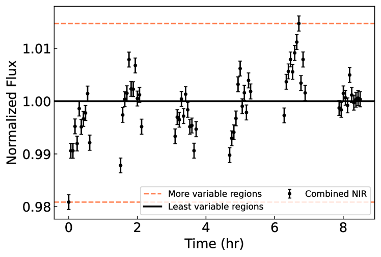
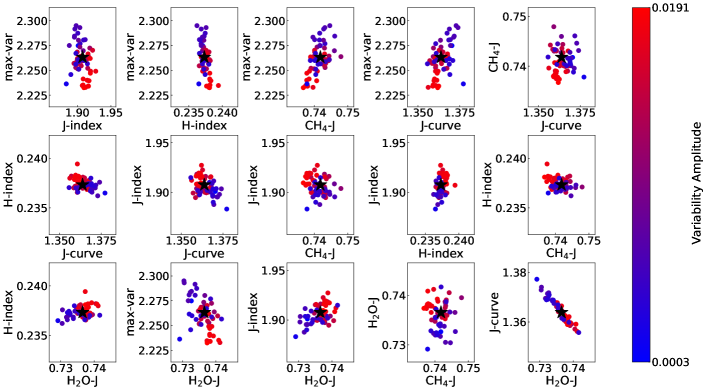
To design our spectral indices, we follow the same procedure as for Oliveros-Gomez et al. (2022). In this Section, we summarize the procedure. In Figure 1 we show the near-infrared white light curve of LP 261-75b as published in Manjavacas et al. (2018). The spectra with the highest variability are those at the extremes of the light curve and those with the lowest variability are those closest to unity. Those spectra will be used in our index method to spot the spectral characteristics that vary the most across the entire spectrum. For this, we produce a template spectrum with the median combining all 66 spectra of the object. This spectrum will be equivalent to a higher signal-to-noise, single-epoch spectrum similar to those normally found in spectral libraries of brown dwarfs. We subtract each of the spectra in the light curve from this template to quantitatively find the differences of each spectrum in each wavelength range concerning the template.
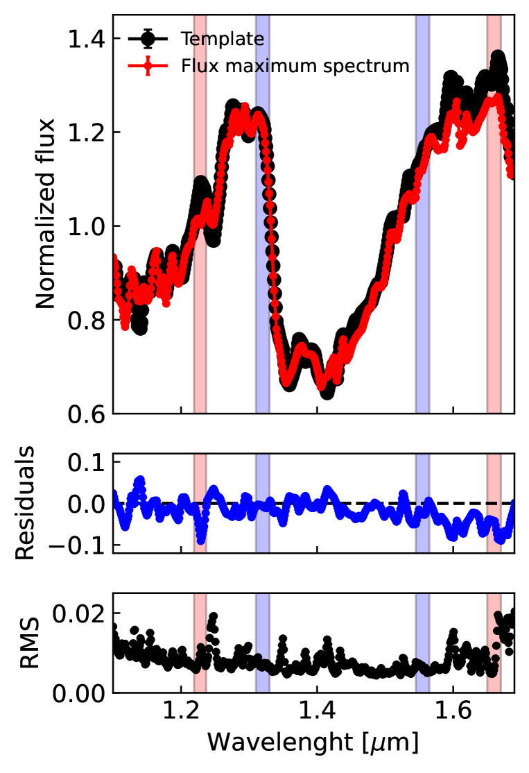
In Figure 2, upper panel, we show the flux maximum spectrum (in red) compared to the template (in black), and their respective residuals at the bottom panel. Windows of 0.03 m width are analyzed every 0.005 m, obtaining the regions of higher and lower variability of the whole wavelength range, indicated in red and blue respectively in Figure 2. With these regions, we define three spectral indices, applying the Equation 1:
| (1) |
Where the highest flux-region, is integrated over the wavelength range in which the residuals are higher. is the integrated flux over the contiguous area over the wavelength range in which the residuals are closer to 0 (contiguous area of minimum variability). We design three new spectral indices, as defined in Table 1, and we add three spectral indices that have been implemented in Burgasser et al. (2006a) and Bardalez Gagliuffi et al. (2014) and which we found helpful to find the flux maximum spectra. We have a total of six spectral indices.
Finally, we apply these indices to all 66 spectra of LP 261-75b, to produce a set of index-index plots as shown in Figure 3. At a glance, we observe that the flux maximum spectra (associated with the outermost part of the light curve in Figure 1) cluster at different areas in the index-index plots than the flux maximum spectra (associated with the values closest to one light curve in the Figure 1). In the upcoming Section, we will objectively define the variable and non-variable areas within the index-index plots using a Machine Learning method.
| Spectral | Numerator Range | Denominator Range | Feature | Reference |
|---|---|---|---|---|
| index | (m) | (m) | ||
| -index | 1.22-1.25 | 1.31-1.335 | Variability in -band | (1) |
| -index | 1.64-1.67 | 1.545-1.575 | Variability in -band | (1) |
| max-var | 1.66-1.69 | 1.34-1.37 | Major difference variability in complete spectra | (1) |
| H2O-J | 1.14–1.165 | 1.26–1.285 | 1.15 m H2O | (2) |
| CH4-J | 1.315 - 1.335 | 1.26–1.285 | 1.32 m CH4 | (2) |
| -curve | 1.26-1.29 | 1.14-1.17 | Curvature across -band | (3) |
4.2 Defining variability areas
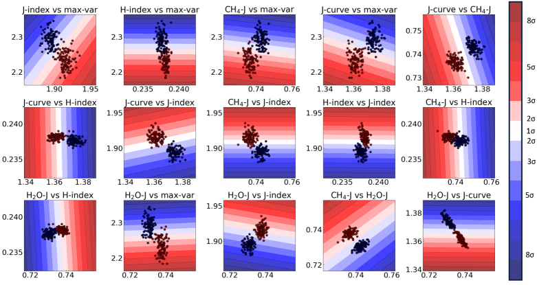
Given that we have a limited amount of spectra for LP 261-75b, before we could robustly define the variable and non-variable areas in the index-index plots in Figure 3, we generated synthetic spectra, similar to the most and flux minimum spectra of LP 261-75b, to further help in the definition of both areas. This is the same method that we followed in Oliveros-Gomez et al. (2022).
We used a Monte Carlo simulation we generated 100 synthetic spectra from the flux minimum spectra of LP 261-75b, and 100 synthetic spectra from the flux maximum spectra. To generate the synthetic spectra, we selected the maximum and minimum flux spectra in the light curve and redefined each of their points in the spectrum using a Gaussian random number generator. The mean value of the Gaussian is the original flux of the spectrum, and the standard deviation is the uncertainty of each point in the sample spectrum. Using this method, we generated 100 synthetic spectra similar to the flux maximum spectra of LP 261-75b, and 100 similar to the flux minimum spectra. Finally, we ran our spectral indices through all synthetic spectra, and we generated new index-index plots (see Figure 4).
To robustly define the variable and non-variable areas of the index-index plots, we use a supervised machine learning method, Support Vector Machine (SVM). To use the SVM method, we must provide a sample containing the points and their value that classifies it to one category or another. We input a sample with the value of each index-index plot for the 200 synthetic spectra created with the Monte Carlo simulation described above, and with the value assigned to it if it is variable (1) or non-variable (0).
The SVM method uses a portion of the sample values as training examples so that it can classify the two groups and evaluate them. This is in order to maximize the gap between the two categories. We use the rest of the sample data to map the space that predicts which category they belong to and evaluate the method.
We used scikit-learn to apply this supervised learning method (Pedregosa et al., 2011) to our data. In addition, we need to select a kernel to apply in our method, to define the forms of pattern the analysis algorithms. Thus, we did kernel variations (linear, radial basis, and polynomial) to define the separation boundaries of the two categories. We decided to use a ‘linear’ kernel because it proposed better-delimited boundaries between the two data sets. We did several tests varying the number and positions of the contour regions to confirm the reliability of finding an object in the variable or non-variable category, until our results stabilize, which determines the sigma value at which our method is reliable.
We note in Figure 4 that the contours separating the two categories are not reliable to classify an object as variable or non-variable (). Thus, we declare objects in the regions and above as being in a reliable variable or non-variable area. Variable areas are shown in red , and non-variable areas are shown in blue ().
Once we define the variable and non-variable areas, we notice with a visual inspection it is possible to observe that some indices seem to have more relevance than others. Therefore, in the Appendix (Section 8), we add some tests to track which combination of indices works best to find the variable and non-variable synthetic spectra.
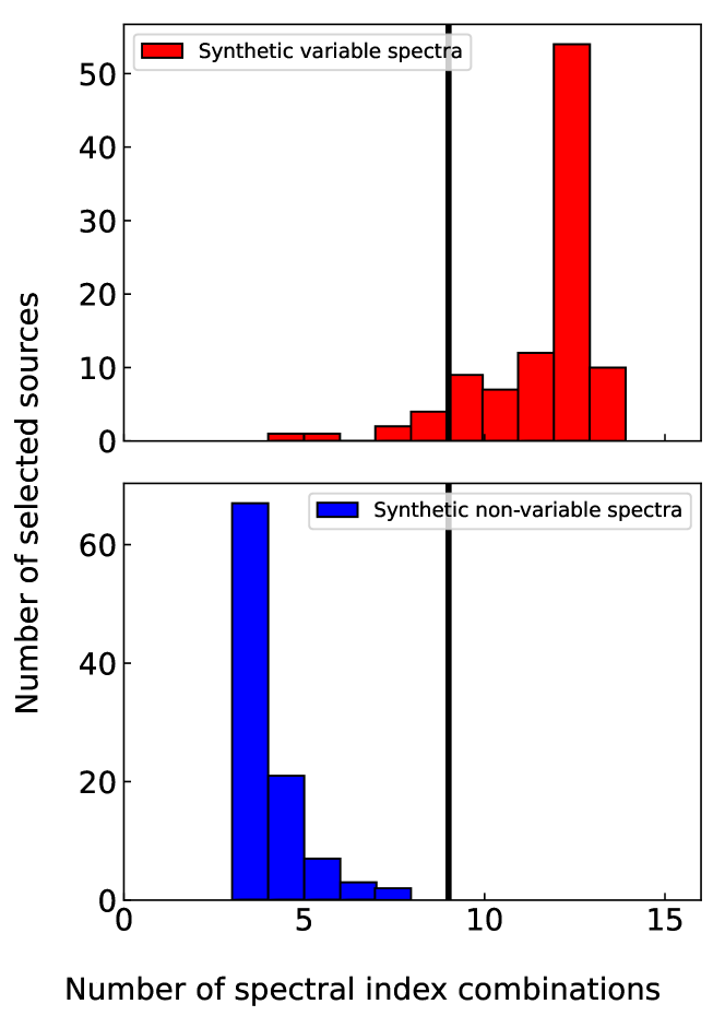
In addition, we generate a histogram that includes the values of the indices calculated for all 200 spectra. It gives us information on how many of the 15 variable areas, each of our spectra is found in (see Figure 5).
We define a variability threshold for the number of index-index plots in which a brown dwarf must be found in the variable zone to be considered a variable candidate. This threshold is 9 of 15 index-index plots. We select this number because for less than 9 plots 100% of the non-variable synthetic spectra are in non-variable areas (see in Figure 5). In addition, in this limit, we obtain 87% of the synthetic variable spectra found in at least 9/15 variable areas. Thus, any brown dwarf that is located in more than 9 index-index plots in the variable areas is considered a variable candidate. The spectra found in less than 9 index-index plots inside variable areas are considered a non-variable candidate.
The Python code to find L4–L8 brown dwarf variable candidates using the spectral indices presented in this work is publically available and ready to be used in Github: https://github.com/ntlucia/BrownDwarf-SpectralIndices.
5 IDENTIFICATION OF VARIABLE CANDIDATES
Once robust variable and non-variable areas were defined within the index-index plots, we used our spectral indices method to identify variable L4–L8 brown dwarf candidates. Since the spectral indices presented here were designed with an L6 dwarf spectrum, these indices apply only to brown dwarfs with two spectral types difference (L4-L8). We applied our indices to a sample of 75 brown dwarfs with a single epoch near-infrared (0.7–2.5 m) spectrum, and spectral type L4-L8 available at the SpeX/IRTF spectral library111https://cass.ucsd.edu/~ajb/browndwarfs/spexprism/html/ldwarf.html (R75-120).
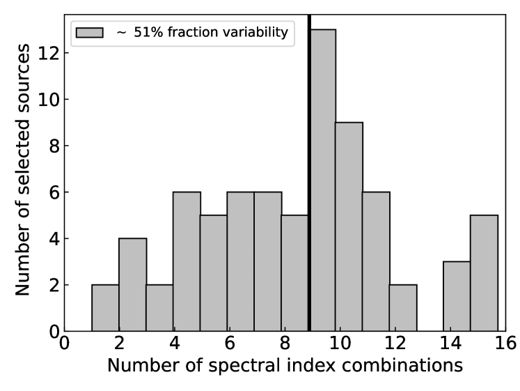
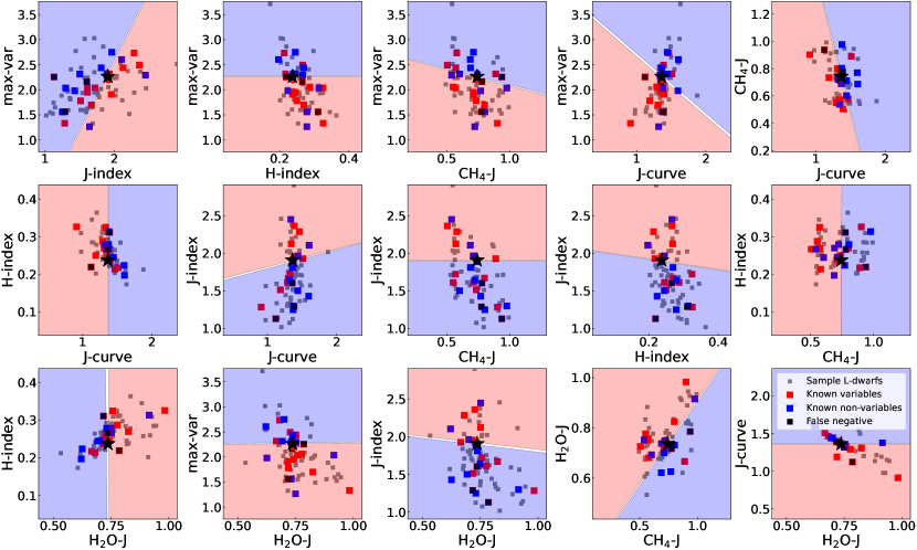
After running our spectral indices on all of them, we concluded that 38 of the 75 L4–L8 brown dwarfs were found as variable candidates (found in 9 or more variable areas). This represents a variability fraction in our L4-L8 sample. In Figure 6, we show the histogram with the number of index-index plots in which each of the objects is found in the variable area.
From our sample, 23 of the 75 objects have been monitored photometrically in the literature, of which 11 are found to be variable (Section 5.1), 9 are found as non-variables in the literature and 3 are found as false negatives (Section 5.2). In the following section, we describe the objects selected as variable and non-variable candidates by our indices. The full list of variable candidates selected by our indices can be found in Table 2.
Including the known variable and non-variable objects that we mention in Table 2, we reproduce a similar analysis of the relevance of the combination of indices. In the Appendix (Section 8), we perform some tests to determine which index-index combinations are more effective in finding variable and non-variable L dwarfs.
| Name | SpeX NIR | Variable | N° | Variability | Variability | Reference | |
|---|---|---|---|---|---|---|---|
| SpT | candidate? | regions | literaturea | -band [%] | 3.6 [%] | variability | |
| L 362-29 B | L5.5 | Yes | 15/15 | ||||
| 2MASS J00282091+2249050 | L7 | No | 05/15 | ||||
| 2MASSW J0030300-145033 | L7 | No | 04/15 | Variable* | 1.52 | (1), (2) | |
| 2MASS J00325937+1410371 | L8 | No | 05/15 | ||||
| LSPM J0036+1821 | L4 | Yes | 09/15 | Variable | 1.22 | (3) | |
| 2MASSI J0103320+193536 | L6 | No | 03/15 | Slow variability | 0.56 | (4), (3) | |
| 2MASSI J0131183+380155 | L4 | Yes | 09/15 | ||||
| 2MASS J01443536-0716142 | L5.5 | Yes | 10/15 | ||||
| 2MASS J01550354+0950003 | L5 | Yes | 09/15 | ||||
| DENIS J020529.0-115925 | L7 | Yes | 11/15 | ||||
| 2MASSW J0208236+273740 | L5 | Yes | 15/15 | ||||
| 2MASS J02425693+2123204 | L4 | No | 06/15 | ||||
| 2MASS J02572581-3105523 | L8 | Yes | 09/15 | ||||
| 2MASSI J0318540-342129 | L7 | Yes | 09/15 | ||||
| 2MASS J04390101-2353083 | L6 | Yes | 14/15 | Variable | 2.6 | (2) | |
| 2MASS J04474307-1936045 | L5 | Yes | 09/15 | ||||
| 2MASS J06244595-4521548 | L5 | Yes | 11/15 | Variable | 1 | (5), (3) | |
| 2MASS J06523073+4710348 | L4.5 | No | 04/15 | ||||
| 2MASS J06540564+6528051 | L6 | Yes | 10/15 | ||||
| 2MASS J07171626+5705430 | L6.5 | Yes | 10/15 | ||||
| 2MASSW J0801405+462850 | L6.5 | No | 8/15 | Non-Variable | (5) | ||
| 2MASS J08053189+4812330 | L4+T5 | Yes | 09/15 | Variable | 1.46 | 3.13 | (6) |
| 2MASSW J0820299+450031 | L5 | No | 04/15 | Slow variability | (4), (3) | ||
| 2MASSI J0825196+211552 | L6 | Yes | 09/15 | Variable | 1 | 1.4 | (5), (4) |
| 2MASS J08350622+1953050 | L4.5 | Yes | 11/15 | ||||
| 2MASS J08354256-0819237 | L5 | Yes | 10/15 | Variable | 1.7 | (2) | |
| 2MASS J08511627+1817302 | L5.5 | No | 07/15 | ||||
| 2MASS J08575849+5708514 | L8 | No | 02/15 | ||||
| 2MASS J09054654+5623117 | L5 | No | 08/15 | ||||
| 2MASS J09083803+5032088 | L7 | No | 08/15 | Non-Variable | (5) | ||
| 2MASS J09153413+0422045 | L7 | Yes | 12/15 | ||||
| 2MASSW J0929336+342952 | L7.5 | No | 04/15 | ||||
| 2MASS J10071185+1930563 | L8 | No | 05/15 | ||||
| 2MASS J10101480-0406499 | L6 | No | 06/15 | Variable* | 5.1 | (3), (9) | |
| 2MASSI J1043075+222523 | L8 | No | 02/15 | ||||
| 2MASS J10433508+1213149 | L7 | Yes | 14/15 | Variable | 1.54 | (3) | |
| 2MASS J10440942+0429376 | L7 | No | 06/15 | ||||
| 2MASS J11040127+1959217 | L4 | Yes | 09/15 | ||||
| HD 97334B | L4.5 | No | 6/15 | ||||
| 2MASS J11211858+4332464 | L7.5 | Yes | 14/15 | ||||
| DENIS J112639.9-500355 | L4.5 | Yes | 09/15 | Variable | 1.2 | 0.21 | (2), (4) |
| 2MASS J11555389+0559577 | L7 | No | 06/15 | Non-variable | (7) | ||
| 2MASS J12195156+3128497 | L8 | No | 06/15 | Non-variable | (5), (3) | ||
| SIPS J1228-1547 | L5.5 | Yes | 12/15 | ||||
| 2MASSW J1239272+551537 | L5 | No | 05/15 | ||||
| 2MASS J13262981-0038314 | L5.5 | No | 01/15 | ||||
| 2MASS J14002320+4338222 | L7 | Yes | 15/15 | ||||
| ULAS2MASS J1407+1241 | L5 | Yes | 15/15 | ||||
| 2MASS J14222720+2215575 | L6.5 | Yes | 09/15 | ||||
| 2MASS J14283132+5923354 | L4 | Yes | 10/15 | ||||
| 2MASSW J1507476-162738 | L5.5 | Yes | 10/15 | Variable | 0.53 | (4), (3) | |
| 2MASSW J1515008+484742 | L6.5 | No | 04/15 | Non-variable | (5) | ||
| 2MASS J15150607+4436483 | L7.5 | No | 07/15 | ||||
| 2MASS J15200224-4422419B | L4.5 | Yes | 12/15 | ||||
| Gl 584c | L8 | No | 01/15 | ||||
| 2MASSI J1526140+204341 | L7 | Yes | 10/15 | ||||
| 2MASS J16303054+4344032 | L7.5 | No | 02/15 | ||||
| 2MASS J16335933-0640552 | L6 | No | 07/15 | ||||
| 2MASS J17054834-0516462 | L4 | Yes | 10/15 | ||||
| 2MASSI J1711457+223204 | L6.5 | No | 08/15 | ||||
| 2MASS J17461199+5034036 | L5 | Yes | 11/15 | ||||
| 2MASS J17502484-0016151 | L5.5 | Yes | 10/15 | Variable | 1.12 | (2), (5), (3) | |
| 2MASS J18212815+1414010 | L5 | Yes | 11/15 | Variable | 0.54 | (4) | |
| 2MASS J19285196-4356256 | L5 | Yes | 11/15 | ||||
| 2MASSI J2002507-052152 | L6 | No | 07/15 | ||||
| 2MASSW J2101154+175658 | L7.5 | No | 02/15 | ||||
| 2MASS J21321145+1341584 | L6 | Yes | 09/15 | ||||
| 2MASSW J2148162+400359 | L6 | No | 03/15 | Slow variability | 1.33 | (4), (3) | |
| 2MASSI J2158045-155009 | L4 | Yes | 09/15 | ||||
| 2MASS J22120703+3430351 | L5 | No | 04/15 | ||||
| 2MASSW J2224438-015852 | L4.5 | No | 07/15 | Non-variable | (4), (3) | ||
| 2MASS J22443167+2043433 | L6.5 | No | 06/15 | Variable* | 5.5 | 0.8 | (7), (3) |
| 2MASS J22521073-1730134 | L7.5 | No | 07/15 | ||||
| 2MASSI J2325453+425148 | L8 | No | 05/15 |
-
•
Notes: a Variable refers to the objects that present any measure variability in the literature, Non-Variable refers to the objects that no measure variability in photospectroscopic studies. slow variability refers to the objects that discuss the small variability, in some cases not consistent or near to the RMS in the measurements. Variable* refers to the false negative in our sample because with our method we obtain non-variable objects. Variability references: (1) Clarke et al. (2008), (2) Radigan et al. (2014), (3) Vos et al. (2020), (4) Metchev et al. (2015), (5) Buenzli et al. (2014), (6) Dupuy & Liu (2012), (7) Koen et al. (2004), (8) Vos et al. (2018), (9) Wilson et al. (2014).
5.1 Variables candidates
The following objects were selected as variable candidates by our indices and have information about their variability in the literature.
5.1.1 LSPM J0036+1821
J0036+1821 is an L4 dwarf (Geballe et al., 2002). It is located at pc (Gaia Collaboration, 2020). Gagné et al. (2015) found an effective temperature of K, and a surface gravity of log(g) = 5.0 dex by fitting the Spectral Energy Distribution (SED) of the object using the BT-Settl atmospheric models. Osorio et al. (2005) was the first to report variability of this object in an -band of 0.25%. Later, Metchev et al. (2015) used J0036+1821 as a control object for recognizing potential activity-induced photometric effects. They found a variability amplitude in the [3.6] Spitzer channel of , and a variability amplitude of in the [4.5] Spitzer channel. They measured a period of hr. Metchev et al. (2015) did not include it as a variable in their final sample since its variability might be associated with magnetic activity. Croll et al. (2016) measured a variability amplitude of . J0036+1821 was found in 9 out of 15 areas in our index–index plots, indicating that it is a variable candidate.
5.1.2 2MASS J04390101-2353083
5.1.3 2MASS J06244595-4521548
J0624-4521 is an L6.5 dwarf (Schneider et al., 2014). It is located at a distance of pc (Gaia Collaboration, 2020). Gagné et al. (2015) found an effective temperature of K, and a surface gravity of log(g) = 5.0 dex by fitting the SED of the object using the BT-Settl atmospheric models.
Buenzli et al. (2014) measured variability of at least 1%, using observations very short, 40 minutes, so they identified variability but did not measure amplitude and period very precisely. J0624-4521 was found in the variable areas in 11 out of 15 of our index–index plots, indicating that it is a variable candidate.
5.1.4 2MASS J08053189+4812330
J0805+4812 was a spectral binary candidate (Burgasser, 2007). It was confirmed as such by Dupuy & Liu (2012). They show large perturbations due to orbital motion with spectral types L4 (primary) + T5 (secondary). J0805+4812 shows variability in their near-IR light curve associated with the transits binary system and not necessarily internal processes of the atmospheres such as clouds (Dupuy & Liu, 2012). Although this system is binary, we use for our analysis the resolved spectrum of the object, the primary dwarf L4.
J0805+4812 was found in the variable areas in 9 out of 15 of our index–index plots, indicating that it is a variable candidate.
5.1.5 2MASSI J0825196+211552
5.1.6 2MASS J08354256-0819237
J0835+1953 is an L5 dwarf (Schneider et al., 2014). It is located at a distance of pc (Schmidt et al., 2010). Gagné et al. (2015) found an effective temperature of K, and a surface gravity of log(g) = 5.0 dex by fitting the SED of the object using the BT-Settl atmospheric models.
Radigan (2014) measured a peak-to-peak variability of 1.3 0.2% using the SofI instrument, installed on the New Technology Telescope (NTT) in -band. J0835+1953 was found in the variable areas in 11 out of 15 of our index–index plots, indicating that it is a variable candidate.
5.1.7 2MASS J10433508+1213149
J1043+1213 is an L7 dwarf (Burgasser et al., 2010). It is located at a distance of pc (Schmidt et al., 2010). Gagné et al. (2015) found an effective temperature of K, and a surface gravity of log(g) = 5.5 dex by fitting the SED of the object using the BT-Settl atmospheric models. Metchev et al. (2015) measured a variability amplitude of , %, with a period hr, but irregular, i. e., the period fits require more Fourier terms than the number of recorded rotations. J1043+1213 was found in the variable areas in 14 out of 15 of our index–index plots, indicating that it is a variable candidate.
5.1.8 DENIS J112639.9-500355
J1126-5003 is an L5.5 dwarf (Phan-Bao et al., 2008). It is located at a distance of pc (Gaia Collaboration, 2020). Folkes et al. (2007) reported that J1126-5003 has unusually blue colors for its L4.5 optical or L6.5 NIR spectral type. Radigan et al. (2014) measured a peak-to-peak variability amplitude in the -band of . Metchev et al. (2015) measured a variability amplitude of , , and they calculated a period of hr with regular periodicity. J1126-5003 was found in the variable areas in 9 out of 15 of our index–index plots, indicating that it is a variable candidate.
5.1.9 2MASSW J1507476-162738
J1507-1627 is an L5V dwarf (Kirkpatrick et al., 2000). It is located at a distance of pc (Gaia Collaboration, 2020). Gagné et al. (2015) found an effective temperature of K, and a surface gravity of log(g) = 5.0 dex by fitting the SED of the object using the BT-Settl atmospheric models.
Metchev et al. (2015) measured a variability amplitude of , , with an irregular period of hr. Metchev et al. (2015) explains that J1507-1627 shows clear spot evolution, since one oscillation appears around 7hr in one channel observing sequence, and continuously grows in amplitude until the end of the other channel sequence, 2.5 hr rotations later. J1507-1627 was found in the variable areas in 10 out of 15 of our index–index plots, indicating that it is a variable candidate.
5.1.10 2MASS J17502484-0016151
J1750-0016 is L5.5 dwarf (Burgasser et al., 2010). It is located at a distance of pc (Gaia Collaboration, 2020). Gagné et al. (2015) found an effective temperature of K, and a surface gravity of log(g) = 4.5 dex by fitting the SED of the object using the BT-Settl atmospheric models.
Buenzli et al. (2014) measured a significant variability in the -band, between 1.12 and 1.32 m, with a period 4hr. However, the variation in the -band is not statistically significant. J1750-0016 was found in the variable areas in 10 out of 15 of our index–index plots, indicating that it is a variable candidate.
5.1.11 2MASS J18212815+1414010
J1821+1414 is an L5 dwarf (Schneider et al., 2014). Gagné et al. (2015) found an effective temperature of K, and a surface gravity of log(g) = 4.5 dex by fitting the SED of the object using the BT-Settl atmospheric models. Looper et al. (2008) classified this object as peculiarly red indicating moderately low gravity, including relative weakness in the alkaline and FeH strengths and sharpness of the -band continuum. Gagné et al. (2014) concluded that despite its signatures of youth this object does not belong to any known young moving group (Faherty et al., 2016).
Metchev et al. (2015) measured a variability amplitude of %, %, and an irregular period of hr. This object is an example of variability in objects with peculiar red spectra or low gravity objects, which are interesting in our sample and are in agreement with other results of spectral indices such as Ashraf et al. (2022) and studied with more detail in Vos et al. (2022). J1821+1414 was found in the variable areas in 11 out of 15 of our index–index plots, indicating that it is a variable candidate.
5.2 Non-variables candidates
In this Section, we list the objects that were selected by our indices as non-variable candidates and are listed as such in the literature.
5.2.1 2MASSI J0103320+193536
J0103+1935 is an L6V (Kirkpatrick et al., 2000) dwarf. It is located at a distance of pc (Faherty et al., 2009). Gagné et al. (2015) found an effective temperature of K, and a surface gravity of log(g) = 5.5 dex by fitting the SED of the object using the BT-Settl atmospheric models.
Metchev et al. (2015) measured a small variability amplitude of % and %. J0103+1935 was found in the variable areas in 3 out of 15 of our index–index plots, indicating that it is a non-variable candidate. Even though J0103+1935 shows some variability, our index method is probably not sensitive to such small variability levels.
5.2.2 2MASSW J0801405+462850
J0801+4628 is an L6.5V dwarf (Kirkpatrick et al., 2000). It is located at a distance of pc (Schmidt et al., 2010). Gagné et al. (2015) found an effective temperature of K, and a surface gravity of log(g) = 5.0 dex by fitting the SED of the object using the BT-Settl atmospheric models.
Buenzli et al. (2014) did not find any significant variability above their uncertainties. J0801+4628 was found in the variable areas in 8 out of 15 of our index–index plots, indicating that it is a non-variable candidate.
5.2.3 2MASSW J0820299+450031
5.2.4 2MASS J09083803+5032088
J0908+5032 is an L8 dwarf (Schneider et al., 2014). It is located at a distance of pc. Gagné et al. (2015) found an effective temperature of K, and a surface gravity of log(g) = 5.5 dex by fitting the SED of the object using the BT-Settl atmospheric models.
Buenzli et al. (2014) did not measure any significant variability above their uncertainties using HST/WFC3 time-resolved spectroscopy. J0908+5032 was found only in 8 out of 15 variable areas of our index–index plots, indicating that it is a non-variable candidate.
5.2.5 2MASS J11555389+0559577
J1155+0559 is an L7.5 dwarf (Knapp et al., 2004). It is located at a distance of pc (Faherty et al., 2012). This object is somewhat controversial and interesting concerning its spectral type and variability, for which they have even cataloged it as L6-L8 peculiar (Gagné et al., 2015). Gizis et al. (2002) noted the presence of emission which can be associated with magnetic fields variability. In addition, Koen (2003) monitored the object for 5 nights of observation, of about 4.6 hr each, in -band, observing variability and obtaining a period of 8 hr.
Koen et al. (2004) monitored J1155+0559 in the - and -bands finding variability with a periodicity of 45 min, which is an extremely short rotational period for a brown dwarf. In this study, J1155+0559 was found in the variable areas in 6 out of 15 of our index–index plots, indicating that it is a non-variable candidate.
5.2.6 2MASS J12195156+3128497
J1219+3128 is an L8 dwarf (Schneider et al., 2014). It is located at a distance of pc (Schmidt et al., 2010). Tannock et al. (2021) found an effective temperature of K, and a surface gravity of log(g) = 5.1 dex by fitting the SED of the object using the BT-Settl and SM08 atmospheric models.
Buenzli et al. (2014) measured a ramp in the 1.12-1.2 m wavelength range, with a small degree of variability, and they presented J1219+3128 as a tentative variable. J1219+3128 was found in the variable areas in 6 out of 15 of our index–index plots, indicating that it is a non-variable candidate.
5.2.7 2MASSW J1515008+484742
J1515+4847 is an L6.5 dwarf (Cruz et al., 2003). It is located at a distance of pc (Gaia Collaboration, 2020). Gagné et al. (2015) found an effective temperature of K, and a surface gravity of log(g) = 5.0 dex by fitting the SED of the object using the BT-Settl atmospheric models.
Buenzli et al. (2014) found no evidence of significant variability in any of the spectral regions for J1515+4847, showing less than 0.5-1% variability per hour, which is within the observational uncertainties. J1515+4847 was found in the variable areas in 4 out of 15 of our index–index plots, indicating that it is a non-variable candidate.
5.2.8 2MASSW J2148162+400359
J2148+4003 is an L7 dwarf (Schneider et al., 2014) at a distance of pc (Gaia Collaboration, 2020), and it is a very red brown dwarf (Looper et al., 2008). Metchev et al. (2015) measured variability of %, %, but in a long observation window (14h). They classify J2148+4003 as non-variable because they only detect flux fluctuations over a long time. J2148+4003 was found in the variable areas in 3 out of 15 of our index–index plots, indicating that it is a non-variable candidate.
5.2.9 2MASSW J2224438-015852
J2224-0158 is an L4.5V dwarf (Kirkpatrick et al., 2000). It is located at a distance of pc (Gaia Collaboration, 2020). Burningham et al. (2021) found an effective temperature of K, and a surface gravity of log(g) = 5.47 dex using atmospheric retrievals.
Metchev et al. (2015) did not find variability on this object. Gelino et al. (2002) did not measure any variability in the -band for J2224-0158. In addition, Burningham et al. (2021) showed us that it has enstatite and quartz clouds, but that the body may have an unfavorable geometry to detect rotational modulation signals, or that the dark regions are arranged latitudinally in bands, and this may be why variability in near-infrared wavelengths is not observed. J2224-0158 was found in the variable areas in 6 out of 15 of our index–index plots, indicating that it is a non-variable candidate.
5.2.10 False Negatives
In this section, we describe the objects that we determine as false negatives because our spectral index method determines them as non-variable objects, but in the literature, they have been measured to have variability in different spectral bands.
2MASSW J0030300-145033: J0030-1450 is an L7 dwarf (Kirkpatrick et al., 2000). It is located at a distance of pc (Faherty et al., 2009). Gagné et al. (2015) found an effective temperature of K, and a surface gravity of log(g) = 5.0 dex by fitting the SED of the object using the BT-Settl atmospheric models.
Enoch et al. (2003) detected periodic variability in -band, with an amplitude of 0.19 mag and period of 1.5 hr. However Clarke et al. (2008) found no evidence of variability, with amplitude smaller than 40 mmag in -band. Similarly, Radigan et al. (2014) observed a flat light curve for this target in the -band throughout 3.2 hr. Vos et al. (2022) found variability of using Spitzer and obtained a period of hr. Therefore, despite discrepancies among the literature results, they are not mutually exclusive. As the observations are not simultaneous, this may be an example where the extent of variability varies over time. J0030-1450 was found in the variable areas in 5 out of 15 of our index–index plots, indicating that it is a non-variable candidate. This may be a false negative of our sample.
2MASS J10101480-0406499: J1010-0406 is field L6 dwarf (Cruz et al., 2003; Reid et al., 2008). It is located at a distance of pc. Gagné et al. (2015) found an effective temperature of K, and a surface gravity of log(g) = 5.0 dex by fitting the SED of the object using the BT-Settl atmospheric models.
Wilson et al. (2014) found a variability amplitude of in an observation window of only 3 hr, using the SofI instrument (band). They did not report a period, because the window observation is too short for a proper determination. J1010-0406 was found in the variable areas in 6 out of 15 of our index–index plots, indicating that it is a non-variable candidate. This is a false negative object in our sample.
2MASS J22443167+2043433: J2244+2043 is an L6.5gamma (Faherty et al., 2016), young and low-gravity dwarf (Gizis et al., 2015). It is located at a distance of pc (Faherty et al., 2009). Faherty et al. (2016) found an effective temperature of K.
Morales-Calderón et al. (2006) and Vos et al. (2018) found variability very close to the RMS amplitude, with Spitzer at 4.5 m of observation and no variability at 3.6 m during 5.7 hr and hr, respectively. In addition, Vos et al. (2018) found no variability in -band during 4hr using UKIRT/WFCAM but they predict with the periodogram a period of hr.
This suggests that the light curves of this object may have evolved in time or that they possess longitudinal bands with sinusoidal surface brightness modulations and an elliptical spot. When two bands have slightly different periods due to different velocities or directions, they interfere to produce a beating between patterns, according to Apai et al. (2017). J2244+2043 was found in the variable areas in 6 out of 15 of our index–index plots, indicating that it is a non-variable candidate.
5.3 New Variable Candidates
The following objects listed in Table 3 are selected as new variable candidates by our spectral indices, not reported before in the literature.
| Name | SpeX NIR | Variable | N° | Distance | References | Additional | ||
|---|---|---|---|---|---|---|---|---|
| SpT | candidate? | regions | [pc] | [K] | [dex] | notes | ||
| L 362-29 B | L5.5 | Yes | 15/15 | 12.1438 0.0376 | 1600 | 5 | (1), (2) | (a) |
| 2MASSI J0131183+380155 | L4 | Yes | 09/15 | 24.4358 0.2956 | (1) | |||
| 2MASS J01443536-0716142 | L5.5 | Yes | 10/15 | 12.7392 0.0804 | 1600 | 5 | (1), (2) | |
| 2MASS J01550354+0950003 | L5 | Yes | 09/15 | 22.2014 0.2687 | 1800 | 4.5 | (1) | |
| DENIS J020529.0-115925 | L7V | Yes | 11/15 | 20.2649 0.6684 | 1500 | 5.5 | (1), (2) | |
| 2MASSW J0208236+273740 | L5V | Yes | 15/15 | 24 2 | 1600 | 5 | (3), (2) | |
| 2MASS J02572581-3105523 | L8 | Yes | 09/15 | 9.7371 0.0451 | ||||
| 2MASSI J0318540-342129 | L7 | Yes | 09/15 | 14.0882 0.3668 | 1600 | 5 | (1), (2) | |
| 2MASS J04474307-1936045 | L5 | Yes | 09/15 | 26 5 | (3), (2) | |||
| 2MASS J06540564+6528051 | L6 | Yes | 10/15 | 38.2 7.5 | 1800 | 5 | (4), (2) | |
| 2MASS J07171626+5705430 | L6.5 | Yes | 10/15 | 28.946 0.4877 | 1700 | 5 | (1), (2) | |
| 2MASS J08354256-0819237 | L5 | Yes | 10/15 | 7.2298 0.0112 | 1800 | 5 | (1),(2) | |
| 2MASS J09153413+0422045 | L7 | Yes | 12/15 | 18.0 4.2 | 1600 | 5.5 | (5), (2) | |
| 2MASS J11040127+1959217 | L4 | Yes | 09/15 | 17.952 0.1245 | 1900 | 5 | (1), (2) | |
| 2MASS J11211858+4332464 | L7.5 | Yes | 14/15 | 46 6 | (3) | |||
| SIPS J1228-1547 | L5.5 | Yes | 12/15 | 21.84 1.8 | 1700 | 5 | (1), (2) | |
| 2MASS J14002320+4338222 | L7 | Yes | 15/15 | 23.7 11.1 | 1600 | 5.5 | (3),(4) | |
| ULAS2MASS J1407+1241 | L5 | Yes | 15/15 | 28.4074 1.2877 | 1600 | 5.5 | (1), (2) | |
| 2MASS J14222720+2215575 | L6.5 | Yes | 09/15 | 31.4 6.4 | (4) | |||
| 2MASS J14283132+5923354 | L4.4V | Yes | 10/15 | 21.949 0.1819 | 1800 | 5.5 | (1),(2) | |
| 2MASS J15200224-4422419B | L4.5 | Yes | 12/15 | 19 1 | (3) | (b) | ||
| 2MASSI J1526140+204341 | L7 | Yes | 10/15 | 20.6983 0.333 | 1600 | 5 | (1),(2) | |
| 2MASS J17054834-0516462 | L4 | Yes | 10/15 | 18.825 0.0852 | 2300 | 5.5 | (1),(2) | |
| 2MASS J17461199+5034036 | L5.7V | Yes | 11/15 | 20.685 0.1914 | 1900 | 5 | (1),(2) | |
| 2MASS J19285196-4356256 | L5 | Yes | 11/15 | 28.59 0.8220 | (1) | |||
| 2MASS J21321145+1341584 | L6 | Yes | 09/15 | 27.77 0.7 | 1500 | 5.5 | (1),(2) | |
| 2MASSI J2158045-155009 | L4 | Yes | 09/15 | 23.197 0.4883 | (1) |
-
•
References (The first one in the column is the distance and the second one is the physical parameters): (1) Gaia Collaboration (2020), (2) Gagné et al. (2015): BT-Settl models, (3) Faherty et al. (2009), (4) Schmidt et al. (2010), (5) Reid et al. (2008). Additional notes: (a) well-separated binary system, (b) well-separated (1.174” 0.016”) binary system.
In Figure 7 we show the distribution in the index-index plots of all the objects in our sample, differentiating between the known variables, non-variables, and false positives (Section 5.1 and 5.2). Also, in Table 2, we show the information of the L4-L8 sample with IRTF/SpeX spectra.
6 Discussion
In this Section, we discuss the results obtained and the relevance for future brown dwarf variability studies.
6.1 Recovery Rates
From the sample of 75 L4–L8 brown dwarfs with IRTF/SpeX spectra, a sub-sample of 23 brown dwarfs was monitored for variability studies in the literature (see Table 2). From those 23 objects, our results show 11 are variable candidates (see Section 5.1), and the other 12 are non-variables candidates (see 5.2). From the sample of 75 L4–L8 brown dwarfs with IRTF/SpeX spectra, a sub-sample of 23 brown dwarfs was found with variability studies in the literature (see Table 2). From those 23 objects, our results show 11 are variable candidates (see Section 5.1), and the other 12 are non-variables candidates (see 5.2). For the 11 variable candidates, the literature reports all of them as variables. Thus, our spectral indices were able to recover 100% of all the variable brown dwarfs, demonstrating the tool’s ability to find the most likely variable brown dwarfs.
Of the 12 non-variable candidates, 9 of them are consistent as non-variable in the literature. But, we obtained three of them, J0030-1450, J0103+1935, and J1010-0406 (Cruz et al., 2003), were classified as non-variable by our spectral indices as it was found in a variable area in less of 9 out of 15 index-index plots and in the literature measure variability in some band of near-infrared, or mid-infrared. Therefore, the recovery rate for variable L4–L8 brown dwarfs for the spectral indices presented here is , also we obtain the false negative rate as 25% (3/12 objects).
This is particularly important to conduct successful rotational modulation campaigns of brown dwarfs, in particular in this spectral range (L4–L8) in which not all brown dwarfs show significant photometric or spectro-photometric variability (see Section 6.3). In this work, we provide the list of the most-likely variable L4–L8 brown dwarfs according to our spectral indices in Section 5.3, and the list of L4–L8 brown dwarfs to avoid in monitoring campaigns in Section 5.1 and5.2.
6.2 Limit of variability detection
In Figure 8, we show a color-magnitude plot of all variable objects in the literature, where we differentiate the percentages of -band and 3.6 m variability, to identify the variability limit that our indices can detect. In Figure 8, we observed how two of the three objects that we report as false negatives (J1010-0406 and J2244+2043), in the literature have variability with values much higher than normally reported. The variability of these objects was measured with ground-based instruments, which are less reliable light curves, since they are more likely contaminated by clouds, telluric absorptions from the atmosphere, etc. This contamination does not happen in light curves obtained with space-based observatories. For the false positives, the variability status has changed with time (See discussion in Section 5.2.10). Thus, for this study, we discard these measurements and define the variability lower limit in 1% for space telescope measurements in 3.6 m, 4.5 m, and -band. However, since for ground-based observations, the variability that is detected depends on the observatory, the telescope size, and the meteorological conditions, we do not define a lower limit for this type of variability reporting.
Additionally, it is worth noting that the 3 false negatives shown in Figure 8 are redder in the -band and of a later type than the bulk of the variables. Although the number of objects we have, is a small number statistic, this may point to a lower effectiveness of our method for later or low-severity objects. However, perhaps this is something we can study in detail in the future.
6.3 Variability Fraction
We estimate the variability fraction in the L4–L8 spectral range using the spectral indices introduced in Section 4 over the sample of 75 L4–L8 brown dwarfs in the IRTF/SpeX spectral library, assuming that in fact, all brown dwarfs flagged as variables by our indices are indeed variable. We compare the variability fraction obtained with our index method to the fraction obtained by other brown dwarf variability surveys in the literature.
In this work, we found that 12 out of the 75 are known variables, flagged as variables by our indices (Section 5.1). In addition, our indices found 27 new variable candidates for which no variability information was available in the literature (Section 5.3). In total, our indices found 38 L4–L8 variable candidates out of the 75 L4–L8 brown dwarfs with IRTF/SpeX spectra (51%). In the literature, only 11 of the 75 are confirmed by variability surveys as variable, bringing the minimum variability fraction to 14% for L4–L8 dwarfs. As in Oliveros-Gomez et al. (2022), we follow the same method as Burgasser et al. (2003) to estimate the maximum variability fraction using a Poisson distribution. We use as the mean of the distribution the percentage of variable candidates found by our indices (51%), and the minimum variable fraction (14%) with the variable objects confirmed in the literature as the minimum of the distribution. We integrated the probability until reaching 0.68 (1- limit) which gives us the upper limit for the variability fraction. Following this procedure, the variability fraction estimated for L4–L8 dwarfs is %.
As we did in Oliveros-Gomez et al. (2022) for mid- and late-T dwarfs, we compare the variability fraction that we obtained with our indices to that calculated by ground-based (Radigan et al., 2014) and space-based brown dwarf variability surveys (Buenzli et al., 2014; Metchev et al., 2015). Radigan et al. (2014) performed a brown dwarf variability survey on 57 L, L/T, and T brown dwarfs using the Du Pont 2.5 m telescope at Las Campanas Observatory and the Canada–France–Hawaii Telescope on Maunakea. Radigan et al. (2014) obtained a variability fraction of % for brown dwarfs outside the L/T transition (L9.0-T3.5), although they do not report a specific variability fraction for the L4–L8 spectral range, this fraction is consistent to that estimated in this work.
Finally, we compare our results to the variability fraction obtained by Buenzli et al. (2014) and Metchev et al. (2015) using the HST/WFC3 instrument and the Spitzer telescope, respectively. Buenzli et al. (2014) monitored a sample of 22 L, L/T, and T dwarfs, and found that four brown dwarfs in the range L5-L8 showed significant or tentative variability out of the 12 dwarfs observed in that spectral range (33%). Metchev et al. (2015) used the [3.6] and [4.5] Spitzer channels, and monitored a sample of L, L/T, and T dwarfs, from which 16 were in the L4–L8 spectral range. Eight out of the 15 L4–L8 brown dwarfs were classified as a variable (50%). After correcting for sensitivity, Metchev et al. (2015) found that % of L dwarfs show variability amplitudes higher than 0.2%. Within uncertainties, our variability fraction is in agreement with the variability fraction estimated by Radigan et al. (2014), Buenzli et al. (2014) and Metchev et al. (2015).
6.4 Physics behind the index method
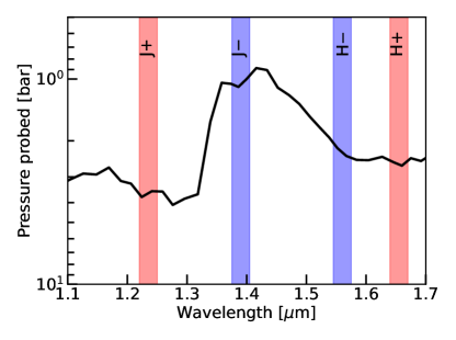
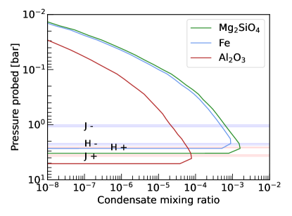
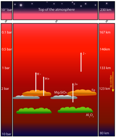
Our spectral indices compare the wavelength ranges of the HST/WFC3 spectrum of LP 261-75b which show the most variability, and the ranges that show the least as the object rotates (see Section 4). As shown in Figure 2 the wavelength ranges that vary the most are between 1.22 and 1.25 m in -band, and between 1.64 and 1.67 m in the -band, and those that vary the least are close to the water band at 1.4 m (1.375-1.405 m and 1.545-1.575 m). To understand why certain wavelength ranges show higher flux variations than others, we use the contribution functions predicted for an object of similar effective temperature and surface gravity by radiative-transfer models (Saumon & Marley, 2008), and also the condensate mixing ratio (mole fraction) of each cloud expected for LP 261-75b (, Fe and ) shown in Fig. 10. In Figure 9 we show the pressure levels probed by HST/WFC3 and the G141 grism for a field L6.0 brown like LP 261–75B ( = 1500 K, log g = 4.5, Bowler et al. 2013) according to radiative-transfer models (Saumon & Marley, 2008).
As observed in Figure 9, the most variable wavelength ranges in the - and -bands (J+ and H+) trace higher pressure levels (deeper) in the atmospheres of mid-L dwarfs. The 1.22–1.25 m region traces the atmosphere of LP 261-75b at 3.64 mbar, and the 1.64-1.67 m region traces the atmosphere at 2.60 mbar. The least variable regions of the spectrum between 1.375-1.405 m and 1.545-1.575 m, trace the 1.04 mbar and 2.27 mbar pressure levels, respectively (- and -). The most variable areas in the - and -bands are tracing a thicker and deeper cloud layer which might introduce higher variability amplitudes in localized wavelength ranges of the HST/WFC3 spectra. On the other hand, the pressure levels traced by the least variable regions are more superficial in comparison, with less cloud coverage present at those atmospheric levels (see Figures 9 and 10), which might explain the lower variability measure on those ranges. As observed in Figure 10, and in Figure 11 for a qualitative representation, the most variable regions of the - and -bands (J+ and H+) trace pressure levels with more cloud coverage, potentially explaining the higher variability measure on those wavelength ranges. Even though the H+ and H- regions trace relatively close pressure levels of LP 261-75B atmosphere, H- is tracing a pressure level with less mole fraction of the cloud likely explaining the smaller variability amplitude found in the H- wavelength range.
6.5 Beyond Brown Dwarf Variability
Brown dwarfs share colors and effective temperatures with some directly-imaged exoplanets (Faherty et al., 2016). Particularly in the mid-to late-L spectral type range, a handful of directly-imaged exoplanets are found with this spectral classification: -Pictoris b (Lagrange et al., 2009), with a = 1650±150 (Bonnefoy et al., 2014a). HIP 65426 b (Chauvin et al., 2017), with a = K (Chauvin et al., 2017). AB-Pictoris b (Chauvin et al., 2005), with a = K and log g = 4.0±0.5 (Bonnefoy et al., 2010), and kap And b (Carson et al., 2013) with a = K (Bonnefoy et al., 2014b).
Time-resolved spectroscopic data provides a wealth of information about the atmospheric dynamic and composition of brown dwarfs, which is most likely due to heterogeneous cloud structures at different pressure levels of the atmospheres of brown dwarfs that evolve within several rotations (Apai et al., 2017). Using radiative-transfer models (Saumon & Marley, 2008) we can infer which types of clouds are introducing the variability found at those pressure levels (Yang et al., 2016; Manjavacas et al., 2021). In addition, if we monitor the object spectroscopically during several rotations, we can infer the map of its surface, and reconstruct which atmospheric characteristics (spots and/or bands) are shaping the light curve produced at different wavelengths (Karalidi et al., 2015; Luger et al., 2019). Time-resolved spectroscopic campaigns have been performed for several dozens of brown dwarfs (Buenzli et al. 2014; Radigan et al. 2014; Metchev et al. 2015; Biller et al. 2018; Manjavacas et al. 2018; Vos et al. 2020, among others), but only for one system of directly-imaged exoplanets HR 8799bc (Apai et al., 2016; Biller et al., 2021) for which only upper levels of variability could be set, due to the low signal-to-noise of the data. Luckily, after the successful launch and commissioning of the James Webb Space Telescope, we are obtaining unprecedented quality spectra for directly-imaged exoplanets. Spectroscopic variability of these objects provides extremely valuable information about the dynamics, clouds, and structure of directly-imaged exoplanets (Hinkley et al., 2022; Patapis et al., 2022; Carter et al., 2023). Nonetheless, to ensure the success of the first rotational monitoring campaigns for directly-imaged exoplanets, spectral indices like those presented in this work might be extremely helpful to pre-select the most likely candidates to show variability. Until now no systematic method to pre-identify variable L dwarfs was available, thus these spectral indices will very likely save hours of expensive telescope time.
7 Conclusions
-
1.
We created novel spectral indices to identify L4–L8 variable candidate brown dwarfs using a single-epoch near-infrared spectrum. For designing these spectral indices, we employed time-resolved HST/WFC3 near-infrared spectra of LP 261-75b, one known variable L6 brown dwarf (Manjavacas et al., 2018).
-
2.
We designed three new spectral indices to find potential L4–L8 variable brown dwarfs. In addition, we used three other spectral indices from previous studies (Burgasser et al., 2010; Bardalez Gagliuffi et al., 2014), to complete a total of six indices. We created 15 index-index plots which allow us to segregate variable and non-variable spectra of LP 261-75b. Using a Monte Carlo simulation of the flux maximum and flux minimum spectra of LP 261-75b we created 100 extra synthetic spectra of both types to clearly define the variable and non-variable areas in the index-index plots. Using a Support Vector Machines (SVM) supervised classification method, we objectively defined the variable and non-variable areas within each index-index plot.
-
3.
We created a histogram showing how many variable or non-variable areas typically each of the variable or non-variable synthetic spectra are found. Using the histogram, we defined the variability threshold in 9/15 index-index plots. The spectra/objects found in more than 9 out of 15 variable areas are classified as variable candidates.
-
4.
We applied our spectral indices to 75 L4–L8 IRTF/SpeX near-infrared spectra, which allowed us to identify potential mid-L variable brown dwarfs. Thirty-eight out of the 75 L4–L8 objects were classified as variable candidates by our spectral indices. Eleven of these objects were reported as known variables in the literature. In addition, we found 27 new variable candidates. With these results, we found a variability fraction of % for our mid-L dwarf sample. Our variability fraction agrees with those provided by Buenzli et al. (2014), Radigan et al. (2014), and Metchev et al. (2015) for the same range of spectral types.
-
5.
From the 37 L4–L8 dwarfs classified as non-variable by our spectral indices, 12 were reported in the literature as non-variables. All of the non-variable objects are non-variable using our method, which represents the 100% recovery rate in non-variable objects. This is crucial since this method will allow us to vet those L4–L8 brown dwarfs that most likely will not show variability in a monitoring campaign.
-
6.
Three objects, J0030-1450, J0103+1935, and J1010-0406 were classified as non-variable by our spectral indices, but it was reported as a variable object in the literature. With these results, the false negative rate is 16%.
-
7.
We report 27 new L4–L8 variable candidates, which will need to be confirmed with near-infrared time-resolved photometry.
-
8.
Given that some L4–L8 dwarfs share effective temperatures and colors with some directly-imaged exoplanets, these spectral indices might be used in the future to find the most likely variable directly-imaged exoplanets to be monitored with the James Webb Space Telescopes or the 30-m type upcoming ground-based telescopes.
N. O. G. acknowledges the support from the Arthur Davidsen Graduate Student Research Fellowship provided by the Space Telescope Science Institute.
J. M. V. acknowledges support from a Royal Society - Science Foundation Ireland University Research Fellowship (URF1221932).
References
- Apai et al. (2021) Apai, D., Nardiello, D., & Bedin, L. R. 2021, ApJ, 906, 64, doi: 10.3847/1538-4357/abcb97
- Apai et al. (2013) Apai, D., Radigan, J., Buenzli, E., et al. 2013, The Astrophysical Journal, 768, 121
- Apai et al. (2016) Apai, D., Kasper, M., Skemer, A., et al. 2016, The Astrophysical Journal, 820, 40
- Apai et al. (2017) Apai, D., Karalidi, T., Marley, M., et al. 2017, Science, 357, 683
- Artigau et al. (2009) Artigau, É., Bouchard, S., Doyon, R., & Lafrenière, D. 2009, ApJ, 701, 1534, doi: 10.1088/0004-637X/701/2/1534
- Ashraf et al. (2022) Ashraf, A., Bardalez Gagliuffi, D. C., Manjavacas, E., et al. 2022, arXiv preprint arXiv:2206.09025
- Bailer-Jones & Mundt (1999) Bailer-Jones, C. A. L., & Mundt, R. 1999, A&A, 348, 800, doi: 10.48550/arXiv.astro-ph/9906439
- Bardalez Gagliuffi et al. (2014) Bardalez Gagliuffi, D. C., Burgasser, A. J., Gelino, C. R., et al. 2014, ApJ, 794, 143, doi: 10.1088/0004-637X/794/2/143
- Bardalez-Gagliuffi et al. (2014) Bardalez-Gagliuffi, D. C., Burgasser, A. J., Gelino, C. R., et al. 2014, The Astrophysical Journal, 794, 143
- Biller et al. (2018) Biller, B. A., Vos, J., Buenzli, E., et al. 2018, AJ, 155, 95, doi: 10.3847/1538-3881/aaa5a6
- Biller et al. (2021) Biller, B. A., Apai, D., Bonnefoy, M., et al. 2021, Monthly Notices of the Royal Astronomical Society, 503, 743
- Bonnefoy et al. (2010) Bonnefoy, M., Chauvin, G., Rojo, P., et al. 2010, A&A, 512, A52, doi: 10.1051/0004-6361/200912688
- Bonnefoy et al. (2014a) Bonnefoy, M., Marleau, G. D., Galicher, R., et al. 2014a, A&A, 567, L9, doi: 10.1051/0004-6361/201424041
- Bonnefoy et al. (2014b) Bonnefoy, M., Currie, T., Marleau, G. D., et al. 2014b, A&A, 562, A111, doi: 10.1051/0004-6361/201322119
- Bowler et al. (2013) Bowler, B. P., Liu, M. C., Shkolnik, E. L., & Dupuy, T. J. 2013, The Astrophysical Journal, 774, 55
- Buenzli et al. (2014) Buenzli, E., Apai, D., Radigan, J., Reid, I. N., & Flateau, D. 2014, The Astrophysical Journal, 782, 77
- Burgasser (2007) Burgasser, A. J. 2007, AJ, 134, 1330, doi: 10.1086/520878
- Burgasser et al. (2006a) Burgasser, A. J., Burrows, A., & Kirkpatrick, J. D. 2006a, The Astrophysical Journal, 639, 1095
- Burgasser et al. (2010) Burgasser, A. J., Cruz, K. L., Cushing, M., et al. 2010, The Astrophysical Journal, 710, 1142
- Burgasser et al. (2006b) Burgasser, A. J., Kirkpatrick, J. D., Cruz, K. L., et al. 2006b, The Astrophysical Journal Supplement Series, 166, 585
- Burgasser et al. (2003) Burgasser, A. J., Kirkpatrick, J. D., Reid, I. N., et al. 2003, ApJ, 586, 512, doi: 10.1086/346263
- Burningham et al. (2021) Burningham, B., Faherty, J. K., Gonzales, E. C., et al. 2021, Monthly Notices of the Royal Astronomical Society, 506, 1944
- Carson et al. (2013) Carson, J., Thalmann, C., Janson, M., et al. 2013, ApJ, 763, L32, doi: 10.1088/2041-8205/763/2/L32
- Carter et al. (2023) Carter, A. L., Hinkley, S., Kammerer, J., et al. 2023, ApJ, 951, L20, doi: 10.3847/2041-8213/acd93e
- Chauvin et al. (2005) Chauvin, G., Lagrange, A. M., Zuckerman, B., et al. 2005, A&A, 438, L29, doi: 10.1051/0004-6361:200500111
- Chauvin et al. (2017) Chauvin, G., Desidera, S., Lagrange, A. M., et al. 2017, A&A, 605, L9, doi: 10.1051/0004-6361/201731152
- Clarke et al. (2008) Clarke, F., Hodgkin, S., Oppenheimer, B., Robertson, J., & Haubois, X. 2008, Monthly Notices of the Royal Astronomical Society, 386, 2009
- Clarke et al. (2008) Clarke, F. J., Hodgkin, S. T., Oppenheimer, B. R., Robertson, J., & Haubois, X. 2008, MNRAS, 386, 2009, doi: 10.1111/j.1365-2966.2008.13135.x
- Croll et al. (2016) Croll, B., Muirhead, P. S., Han, E., et al. 2016, Long-term, Multiwavelength Light Curves of Ultra-cool Dwarfs: I. An Interplay of Starspots & Clouds Likely Drive the Variability of the L3.5 dwarf 2MASS 0036+18. https://arxiv.org/abs/1609.03586
- Cruz et al. (2003) Cruz, K. L., Reid, I. N., Liebert, J., Kirkpatrick, J. D., & Lowrance, P. J. 2003, The Astronomical Journal, 126, 2421
- Dupuy & Liu (2012) Dupuy, T. J., & Liu, M. C. 2012, The Astrophysical Journal Supplement Series, 201, 19
- Enoch et al. (2003) Enoch, M. L., Brown, M. E., & Burgasser, A. J. 2003, The Astronomical Journal, 126, 1006
- Faherty et al. (2009) Faherty, J. K., Burgasser, A. J., West, A. A., et al. 2009, The Astronomical Journal, 139, 176
- Faherty et al. (2012) Faherty, J. K., Burgasser, A. J., Walter, F. M., et al. 2012, The Astrophysical Journal, 752, 56
- Faherty et al. (2016) Faherty, J. K., Riedel, A. R., Cruz, K. L., et al. 2016, The Astrophysical Journal Supplement Series, 225, 10
- Folkes et al. (2007) Folkes, S. L., Pinfield, D. J., Kendall, T. R., & Jones, H. R. 2007, Monthly Notices of the Royal Astronomical Society, 378, 901
- Gagné et al. (2015) Gagné, J., Burgasser, A. J., Faherty, J. K., et al. 2015, ApJ, 808, L20, doi: 10.1088/2041-8205/808/1/L20
- Gagné et al. (2014) Gagné, J., Lafrenière, D., Doyon, R., Malo, L., & Artigau, É. 2014, The Astrophysical Journal, 783, 121
- Gagné et al. (2015) Gagné, J., Faherty, J. K., Cruz, K. L., et al. 2015, The Astrophysical Journal Supplement Series, 219, 33
- Gaia Collaboration (2020) Gaia Collaboration. 2020, VizieR Online Data Catalog, I/350
- Geballe et al. (2002) Geballe, T., Knapp, G., Leggett, S., et al. 2002, The Astrophysical Journal, 564, 466
- Gelino et al. (2002) Gelino, C. R., Marley, M. S., Holtzman, J. A., Ackerman, A. S., & Lodders, K. 2002, The Astrophysical Journal, 577, 433
- Gizis et al. (2015) Gizis, J. E., Allers, K. N., Liu, M. C., et al. 2015, The Astrophysical Journal, 799, 203
- Gizis et al. (2002) Gizis, J. E., Reid, I. N., & Hawley, S. L. 2002, The Astronomical Journal, 123, 3356
- Hinkley et al. (2022) Hinkley, S., Carter, A. L., Ray, S., et al. 2022, PASP, 134, 095003, doi: 10.1088/1538-3873/ac77bd
- Karalidi et al. (2015) Karalidi, T., Apai, D., Schneider, G., Hanson, J. R., & Pasachoff, J. M. 2015, The Astrophysical Journal, 814, 65
- Kirkpatrick et al. (2000) Kirkpatrick, J. D., Reid, I. N., Liebert, J., et al. 2000, The Astronomical Journal, 120, 447
- Knapp et al. (2004) Knapp, G., Leggett, S. K., Fan, X., et al. 2004, The Astronomical Journal, 127, 3553
- Koen (2003) Koen, C. 2003, Monthly Notices of the Royal Astronomical Society, 346, 473
- Koen et al. (2004) Koen, C., Matsunaga, N., & Menzies, J. 2004, Monthly Notices of the Royal Astronomical Society, 354, 466
- Lagrange et al. (2009) Lagrange, A. M., Gratadour, D., Chauvin, G., et al. 2009, A&A, 493, L21, doi: 10.1051/0004-6361:200811325
- Looper et al. (2008) Looper, D. L., Kirkpatrick, J. D., Cutri, R. M., et al. 2008, The Astrophysical Journal, 686, 528
- Luger et al. (2019) Luger, R., Agol, E., Foreman-Mackey, D., et al. 2019, AJ, 157, 64, doi: 10.3847/1538-3881/aae8e5
- Manjavacas et al. (2021) Manjavacas, E., Karalidi, T., Vos, J. M., Biller, B. A., & Lew, B. W. 2021, The Astronomical Journal, 162, 179
- Manjavacas et al. (2018) Manjavacas, E., Apai, D., Zhou, Y., et al. 2018, The Astronomical Journal, 155, 11
- Metchev et al. (2015) Metchev, S. A., Heinze, A., Apai, D., et al. 2015, The Astrophysical Journal, 799, 154
- Morales-Calderón et al. (2006) Morales-Calderón, M., Stauffer, J., Kirkpatrick, J. D., et al. 2006, The Astrophysical Journal, 653, 1454
- Oliveros-Gomez et al. (2022) Oliveros-Gomez, N., Manjavacas, E., Ashraf, A., et al. 2022, The Astrophysical Journal, 939, 72
- Oppenheimer et al. (1995) Oppenheimer, B. R., Kulkarni, S. R., Matthews, K., & Nakajima, T. 1995, Science, 270, 1478, doi: 10.1126/science.270.5241.1478
- Osorio et al. (2005) Osorio, M. Z., Caballero, J., & Béjar, V. 2005, The Astrophysical Journal, 621, 445
- Patapis et al. (2022) Patapis, P., Nasedkin, E., Cugno, G., et al. 2022, A&A, 658, A72, doi: 10.1051/0004-6361/202141663
- Pedregosa et al. (2011) Pedregosa, F., Varoquaux, G., Gramfort, A., et al. 2011, Journal of Machine Learning Research, 12, 2825
- Phan-Bao et al. (2008) Phan-Bao, N., Bessell, M., Martín, E., et al. 2008, Monthly Notices of the Royal Astronomical Society, 383, 831
- Radigan (2014) Radigan, J. 2014, The Astrophysical Journal, 797, 120
- Radigan et al. (2014) Radigan, J., Lafrenière, D., Jayawardhana, R., & Artigau, E. 2014, The Astrophysical Journal, 793, 75
- Rebolo et al. (1995) Rebolo, R., Zapatero Osorio, M. R., & Martín, E. L. 1995, Nature, 377, 129, doi: 10.1038/377129a0
- Reid et al. (2008) Reid, I. N., Cruz, K. L., Kirkpatrick, J. D., et al. 2008, The Astronomical Journal, 136, 1290
- Reid & Walkowicz (2006) Reid, I. N., & Walkowicz, L. M. 2006, Publications of the Astronomical Society of the Pacific, 118, 671
- Saumon & Marley (2008) Saumon, D., & Marley, M. S. 2008, ApJ, 689, 1327, doi: 10.1086/592734
- Schmidt et al. (2010) Schmidt, S. J., West, A. A., Hawley, S. L., & Pineda, J. S. 2010, The Astronomical Journal, 139, 1808
- Schneider et al. (2014) Schneider, A. C., Cushing, M. C., Kirkpatrick, J. D., et al. 2014, The Astronomical Journal, 147, 34
- Suarez et al. (2023) Suarez, G., Vos, J. M., Metchev, S., Faherty, J. K., & Cruz, K. 2023, arXiv e-prints, arXiv:2308.02093, doi: 10.48550/arXiv.2308.02093
- Tan & Showman (2021) Tan, X., & Showman, A. P. 2021, MNRAS, 502, 2198, doi: 10.1093/mnras/stab097
- Tannock et al. (2021) Tannock, M. E., Metchev, S., Heinze, A., et al. 2021, The Astronomical Journal, 161, 224
- Tremblin et al. (2016) Tremblin, P., Amundsen, D. S., Chabrier, G., et al. 2016, The Astrophysical journal letters, 817, L19
- Tremblin et al. (2015) Tremblin, P., Amundsen, D. S., Mourier, P., et al. 2015, The Astrophysical Journal Letters, 804, L17
- Vos et al. (2017) Vos, J. M., Allers, K. N., & Biller, B. A. 2017, ApJ, 842, 78, doi: 10.3847/1538-4357/aa73cf
- Vos et al. (2018) Vos, J. M., Allers, K. N., Biller, B. A., et al. 2018, Monthly Notices of the Royal Astronomical Society, 474, 1041
- Vos et al. (2022) Vos, J. M., Faherty, J. K., Gagné, J., et al. 2022, ApJ, 924, 68, doi: 10.3847/1538-4357/ac4502
- Vos et al. (2022) Vos, J. M., Faherty, J. K., Gagné, J., et al. 2022, The Astrophysical Journal, 924, 68
- Vos et al. (2020) Vos, J. M., Biller, B. A., Allers, K. N., et al. 2020, The Astronomical Journal, 160, 38
- Wilson et al. (2014) Wilson, P., Rajan, A., & Patience, J. 2014, Astronomy & Astrophysics, 566, A111
- Yang et al. (2016) Yang, H., Apai, D., Marley, M. S., et al. 2016, The Astrophysical Journal, 826, 8
8 Appendix
In our visual inspection of the Figures 3 and 4, we noticed that some index-index combinations seemed more important than others in finding variable or non-variable objects. Here we show which index-index combinations are more relevant than others.
8.1 Relevance of each index-index combination
To test which of the index-index combinations presented in Section 4 are more relevant to find variable or non-variable L dwarfs, we measured the number of variable and non-variable spectra that fall into each of the variability regions in all the possible combinations of the indices. We applied this methodology to both the variable and non-variable synthetic spectra shown in Figure 4, as well as to all known variable and non-variable objects in the literature (red and blue squares in Figure 7, respectively).
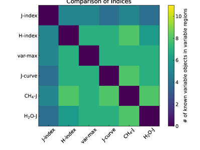
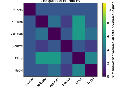
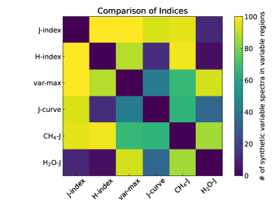
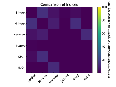
In Figure 12, we show the 6x6 matrix of all possible index-index combinations. In this plot, the color map represents the number of variables (Fig. 12 - left) and non-variable synthetic spectra (Fig. 12 - right) falling within the variability regions in the index-index plots defined in Section 4.
In Figure 12, we noticed that the combination of H2O-J index vs J- and H-indices seem less effective than the others in finding variable brown dwarfs. However, in Figure 12, right we see that all index-index combinations, including H2O-J index vs J- and H-indices can find non-variable spectra. Therefore, we concluded that all index-index combinations of indices are necessary to find either variable or non-variable spectra.
Following the same methodology explained previously, we use the spectra of the known variables in the literature (Figure 13, left), and the spectra of the known non-variable (Fig. 13, left), and we explore which index-index combinations are able to find most of the known variable and non-variable objects. For this case of known objects, we see that the distribution is a little different since it seems that most index-index combinations are the same efficient at finding variable and non-variable objects.