Numerical simulation of the Gross–Pitaevskii equation via vortex tracking

Abstract.

This paper deals with the numerical simulation of the Gross–Pitaevskii (GP) equation, for which a well-known feature is the appearance of quantized vortices with core size of the order of a small parameter $\varepsilon$. Without a magnetic field and with suitable initial conditions, these vortices interact, in the singular limit $\varepsilon\to 0$, through an explicit Hamiltonian dynamics. Using this analytical framework, we develop and analyze a numerical strategy based on the reduced-order Hamiltonian system to efficiently simulate the infinite-dimensional GP equation for small, but finite, $\varepsilon$. This method allows us to avoid numerical stability issues in solving the GP equation, where small values of $\varepsilon$ typically require very fine meshes and time steps. We also provide a mathematical justification of our method in terms of rigorous error estimates of the error in the supercurrent, together with numerical illustrations.

1. Introduction

1.1. Model and motivations

Gross–Pitaevskii equations (GP) are a class of nonlinear Schrödinger equations for quantum mechanical many particle systems in terms of a complex-valued field $u$, featured e.g. in Bose–Einstein condensation, superconductivity and other condensed matter systems. A prototypical form of GP arises from the usual Ginzburg–Landau Hamiltonian of a super-fluid

$$E_{\varepsilon}(u)=\int_{\Omega}e_{\varepsilon}(u)\quad\text{with}\quad e_{\varepsilon}(u)=\frac{1}{2}|\nabla u|^{2}+\frac{1}{4\varepsilon^{2}}(1-|u|^{2})^{2}\,$$ (1)

on a simply connected smoothly bounded domain $\Omega\subset\mathbb{R}^{2}$. The mathematical investigation of the variational model and its minimizers in the singular limit $\varepsilon\to 0$ has been initiated in the seminal work [9]. The corresponding Schrödinger flow $\imath\partial_{t}\psi=-\nabla_{L^{2}}E_{\varepsilon}(\psi)$ (with $\imath$ the imaginary unit), on a smooth bounded domain $\Omega\subset\mathbb{R}^{2}$ with homogeneous Neumann boundary conditions, has the form

$$\begin{cases}\displaystyle\imath\partial_{t}\psi_{\varepsilon}(x,t)=\Delta\psi_{\varepsilon}(x,t)+\frac{1}{\varepsilon^{2}}\left(1-\left|\psi_{\varepsilon}(x,t)\right|^{2}\right)\psi_{\varepsilon}(x,t),\quad x\in\Omega,\\ \psi_{\varepsilon}(x,0)=\psi_{\varepsilon}^{0}(x)\quad x\in\Omega,\\ \partial_{\nu}\psi_{\varepsilon}(x,t)=0\quad x\in\partial\Omega,\ t\geq 0,\end{cases}$$ (2)

where $\psi_{\varepsilon}^{0}\in H^{1}(\Omega,\mathbb{C})$ and $\nu$ is the outward normal to the boundary $\partial\Omega$. Note that, because of the homogeneous Neumann boundary condition, the energy $E_{\varepsilon}(\psi_{\varepsilon})$ is preserved: $E_{\varepsilon}(\psi_{\varepsilon}(t))=E_{\varepsilon}(\psi_{\varepsilon}^{0})$ for all $t\geq 0$. In this context $|\psi|^{2}$ is interpreted as the density, and other physical quantities such as the supercurrents $j(\psi)=\frac{1}{2\imath}(\overline{\psi}\nabla\psi-\psi\nabla\overline{\psi})$ and the vorticity $J\psi=\frac{1}{2}\nabla\times j(\psi)$ can be defined.

A striking feature of super-fluids is the occurrence of quantized vortices that evolve to leading order according to the ODE system known for point vortices in an ideal incompressible fluid. This behavior has been predicted by formal analysis in physics [16] and verified by matched asymptotics in applied mathematics literature [15, 31]. The mathematical link is the Madelung transform which is known to relate Schrödinger equations in quantum mechanics and Euler equations in fluid mechanics. The rigorous description of vortex dynamics arising from GP in the variational framework of [9] has been established in [12, 30], see also [32]. It considers a family of solutions $\psi_{\varepsilon}$ to (2) with initial data $\psi^{0}_{\varepsilon}$ for which the vorticity converges to a sum of point masses at distinct points (vortex locations) $a^{0}_{j}\in\Omega$ with a single quantum of vorticity $d_{j}=\pm 1$, i.e.

$$J\psi^{0}_{\varepsilon}\to\pi\sum_{j=1}^{N}d_{j}\delta_{a^{0}_{j}}$$ (3)

weakly in the sense of measures. Suitable norms to control this convergence include the $\dot{W}^{-1,1}$ norm dual to the Lipschitz norm, closely related to minimal connection and the $1$-Wasserstein distance. A further key assumption is the so-called “well-preparedness” of initial conditions, i.e. initial energies are asymptotically minimal given boundary conditions, vortex locations $a_{j}^{0}$ and vorticities $d_{j}$ as above. The result is that $J\psi_{\varepsilon}(t)\to\pi\sum_{j=1}^{N}d_{j}\delta_{a_{j}(t)}$ for $t>0$ where the singular points $\bm{a}(t)=(a_{1}(t),...,a_{N}(t))$ of degree $d=(d_{1},...,d_{N})$ solve the point vortex system

$$\begin{cases}\dot{a}_{j}(t)=-\frac{1}{\pi}d_{j}\mathbb{J}\nabla_{a_{j}}W({\bm{a}}(t),d),\\ {a}_{j}(0)={a}^{0}_{j},\end{cases}\quad\text{with}\quad\mathbb{J}=\begin{bmatrix}0&1\\ -1&0\end{bmatrix},$$ (4)

with the standard symplectic matrix $\mathbb{J}\in\mathbb{R}^{2N\times 2N}$ and the two-dimensional Coulomb-type Hamiltonian

$$W({\bm{a}},{d})=-{\pi}\sum_{1\leq i\neq j\leq N}d_{i}d_{j}\ln|a_{i}-a_{j}|+\mbox{boundary terms}.$$ (5)

For $\Omega=\mathbb{R}^{2}$ in the absence of boundary conditions, this Hamiltonian system is classical and well-understood. The general case of a bounded domain $\Omega$ is more subtle and recently became a topic of intense investigations particularly regarding the existence of periodic solutions, see e.g. [8].

From a variational point of view, $W$ is the renormalized energy introduced in [9], corresponding to the $\Gamma$ - limit of the Ginzburg–Landau energy (1) minus the logarithmically diverging self-energy of $N$ vortices of degree $d_{j}=\pm 1$:

$$E_{\varepsilon}(u_{\varepsilon})-N\left(\pi\ln(1/\varepsilon)+\gamma\right)\approx W({\bm{a}},{d})\quad\text{as}\quad\varepsilon\to 0,$$ (6)

for an explicit constant $\gamma>0$, with respect to the convergence (3). Results also characterize the asymptotic limits of the supercurrents $j(\psi_{\varepsilon}(t))$ in $L^{p}(\Omega)$ and of the wave functions $\psi_{\varepsilon}(t)$ in $W^{1,p}(\Omega)$ for $p<2$, respectively, towards $u^{*}(t)$ with values in $\mathbb{S}^{1}$ having point singularities at the site of vortex locations $\bm{a}(t)$. More precisely, $u^{*}=u^{*}(\cdot;\bm{a},d)\in\mathbb{S}^{1}$ is the uniquely determined harmonic map with singularities at locations $\bm{a}$ with local degrees $d$, and with boundary conditions. These so-called canonical harmonic maps have the explicit form

$$u^{*}(x;{\bm{a}},{d})=e^{\imath H(x)}\prod_{j=1}^{N}\left(\frac{x-a_{j}}{|x-a_{j}|}\right)^{d_{j}},\qquad x\in\Omega\subset\mathbb{R}^{2}\simeq\mathbb{C},$$ (7)

for a harmonic phase function $H\in C^{\infty}(\overline{\Omega})$ such that the boundary conditions are satisfied. While GP is globally (in time) well-posed in appropriate function spaces (see for instance [17, 18] and references therein), the asymptotic results are only valid up to the first time of collision of the point vortex system which may happen in finite time. A substantial improvement of the above asymptotic results has been obtained in [25], which establish a quantitative description based on largely improved Jacobian and supercurrents estimates. This proves that the vortex motion law holds approximately for small but finite $\varepsilon$, rather than in the limit $\varepsilon\to 0$, and is accompanied by an estimate of the rate of convergence and the time interval for which the results remain valid.

On the other hand, the numerical approximation of solutions of equation (2) is a well-established research field. There is a variety of numerical methods to solve nonlinear Schrödinger equations such as equation (2). A comprehensive overview of the main numerical methods to simulate such equations can be found in [2], where the most common time-space-discretization strategies are compared and different properties listed. The large majority of numerical methods employ time-splitting strategies together with a uniform spatial approximation, either by the Fourier (pseudo-)spectral, finite element or finite difference method, see e.g. [1, 4, 5, 6, 7, 10, 27, 37] and references inside, to mention a few of the many contributions. From a perspective of approximation theory, such methods are of course fine as long as the solutions are smooth during the simulation. In the regime of small values of $\varepsilon$, which is the regime that we target in this paper, this becomes delicate in terms of accuracy. For irregular solutions containing singularities, it is common practice in numerical analysis and scientific computing to perform mesh refinements. In the case of finite element approximations, this leads to so-called adaptive finite element methods which require an element-wise quantification of the error over the mesh, which is typically achieved by considering the residual of the PDE and results in residual-based a posteriori estimators. Interestingly, the numerical study presented in [36] demonstrates superiority of the Fourier (pseudo-) spectral method with adaptive higher-order time-splitting schemes over an adaptive finite element method with local time-stepping. However, this paper is limited to the case of the semi-classical limit (i.e. when the left-hand side of (2) is multiplied by $1/\varepsilon$). In the case of discrete minimizers of the Ginzburg–Landau energy, recent works [13] highlighted, by rigorous a priori bounds in suitable Sobolev norms, the necessity of very fine element mesh when the model parameter $\varepsilon$ is small. Additionally, in [6, 7], the authors propose a numerical study of the vortex interaction for different types of nonlinear Schrödinger equations. They compare the vortex trajectory for finite and small $\varepsilon$ to the one given by the effective dynamics (4), providing a numerical illustration of the singular limit $\varepsilon\to 0$.

These considerations motivate the search for novel numerical methods, taking advantages of the known (low-dimensional) ODE in the singular limit $\varepsilon\to 0$ in order to approximate the solution to the GP equation (2) for small, but finite, $\varepsilon$. The idea we develop in this paper is based on the construction of “well-prepared” initial conditions presented in [25], where the authors suggest to construct such initial conditions by smoothing out the canonical harmonic map with provided vortex locations. From an abstract perspective, this gives rise to a nonlinear projection $\mathcal{P}_{\varepsilon}:(\bm{a},d)\in\Omega^{N}\times\left\{\pm 1\right\}^{N}\mapsto u^{*}_{\varepsilon}(\bm{a},d)$ on $N$-dimensional submanifolds $M^{\varepsilon}\subset H^{1}(\Omega;\mathbb{C})$ defined by $M^{\varepsilon}=\{u_{\varepsilon}^{*}=u_{\varepsilon}^{*}(x;\bm{a},d):\bm{a}\in\Omega^{N}\}\cong\Omega^{N}$ of elements $u_{\varepsilon}^{*}$ obtained from smoothing out canonical harmonic maps $u^{*}=u^{*}(x;\bm{a},d)$ corresponding to vortices at $\bm{a}\in\Omega^{*N}$ and with $d=\{\pm 1\}^{N}$ fixed in an energetically optimal fashion such that

$$\left\|Ju_{\varepsilon}^{*}-\pi\sum_{j=1}^{N}d_{j}\delta_{a_{j}}\right\|_{\dot{W}^{-1,1}}\lesssim\varepsilon^{\alpha}\quad\text{and}\quad\|j(u_{\varepsilon}^{*})-j(u^{*}(\bm{a},d))\|_{L^{\frac{4}{3}}}\lesssim\varepsilon^{\gamma},$$ (8)

for some $\alpha,\gamma\in(0,1)$. The result of [25] is that such a projection can be defined in a (tubular) neighborhood of $M^{\varepsilon}$. Moreover, if vortices are moved according to (4), the estimates remain valid for the GP solution, giving rise to space-time projection onto a subspace in terms of vortex trajectories. In other terms, well-preparedness is conserved in the time interval for which these estimates are valid: in this paper we suggest to use this property to recover an approximation of the solution $\psi_{\varepsilon}$ to the GP equation at time $t>0$. The main idea is, starting from a well-prepared initial condition $\psi^{0}_{\varepsilon}$, to evolve the vortices according to the Hamiltonian ODE (4) up to some time $t$. Then, by the same projection used to set-up well-prepared initial conditions, build back an approximation $\psi_{\varepsilon}^{*}(t)$ of $\psi_{\varepsilon}(t)$ by smoothing out the canonical harmonic map with singularities given by the vortex locations at time $t$. Numerically, the time consuming step is thus the computation of the solutions to the Hamiltonian dynamics (4), which can done in a few seconds on a personal laptop, a significant improvement with respect to the simulation of the full PDE (2) for very small $\varepsilon$. However, the analytical framework of the singular limit being valid as long as the vortices stay away from each other, our method cannot be used to reproduce nonlinear effects such as radiation and sound waves triggered by vortex collisions. Finally, the main contributions of this paper can be summarized as follows:

• We propose, and implement, a new method to approximate numerically the solution to (2) in the regime of small, but finite, $\varepsilon$, with numerical evidence of its accuracy. We also propose an efficient and cheap way to solve the Hamiltonian ODE (4) by using harmonic polynomials to evaluate the boundary terms in the renormalized energy $W$ defined in (5), which involve the resolution of a Laplace equation.

• We prove that our method is asymptotically exact when $\varepsilon\to 0$ together with the discretization parameters by deriving an a priori bound on the supercurrents, using the results from [25] and classical elliptic estimates.

1.2. Structure of the paper

This paper is organized as follows. First, we conclude this introductory section with some general notations. Then, in Section 2, we present a short review of the analytical results on the limit $\varepsilon\to 0$, as well as the notion of well-prepared initial conditions. In Section 3, we detail the numerical resolution of the vortex trajectories as solutions of the Hamiltonian ODE (4), together with some numerical experiments. Finally, in Section 4, we present our new method, based on vortex tracking. We also provide an a priori bound of the error on the supercurrents in terms of $\varepsilon$ and the discretization parameters, with a numerical illustration of this bound.

1.3. Notations

In this paper and the numerical simulations we present, we consider a domain $\Omega$ which is a bounded, simply connected, open subset of $\mathbb{R}^{2}$ with smooth boundary. We denote by $\nu$ the (unit) outward normal to $\Omega$ and by $\tau$ the tangential vector such that the basis $(\nu,\tau)$ is direct. Vortices are considered as point-like defects in the bounded domain $\Omega$: we will use throughout the paper the notation $\bm{a}^{0}=(a^{0}_{j})_{j=1,\dots,N}\in\Omega^{*N}$, ${\bm{a}}(t)=(a_{j}(t))_{j=1,\dots,N}\in\Omega^{*N}$ and $d=(d_{j})_{j=1,\dots,N}\in\left\{\pm 1\right\}^{N}$ to describe the positions (at time $t=0$ and $t>0$) and the degrees of $N$ vortices. Here, $\Omega^{*N}=\left\{\bm{a}\in\Omega,\ a_{i}\neq a_{j},\ \forall\ 1\leq i\neq j\leq N\right\}$. Moreover, time-dependent wave functions will be denoted by $\psi$ or $\psi(t):\Omega\to\mathbb{C}$ for their evaluation at time $t$ while $u_{\varepsilon}$ and $u^{*}$ are used to denote respectively minimizers of the Ginzburg–Landau energy $E_{\varepsilon}$ and canonical harmonic maps.

We will often use the notation $A\lesssim B$ to indicate the existence of a constant $C>0$ such that $A\leq CB$. If the constant $C$ depends on some additional parameter (e.g. , $\varepsilon$), then we use the notation $A\lesssim_{\varepsilon}B$ to emphasize this dependence.

When no ambiguity occurs, $x\in\mathbb{R}^{2}$ is identified with the complex number $x_{1}+\imath x_{2}\in\mathbb{C}$. For $x\in\mathbb{R}^{2}$, $|x|$ is the Euclidean norm of $x$ and $\theta(x)$ is the unique element of $(-\pi,\pi]$ representing the equivalence class of $\arg(x)$. For $x=(x_{1},x_{2}),y=(y_{1},y_{2})\in\mathbb{R}^{2}$, $x\times y=x_{1}y_{2}-x_{2}y_{1}$. If $w:\mathbb{R}^{2}\to\mathbb{R}^{2}$, we define $\nabla\times w=\partial_{x_{1}}w_{2}-\partial_{x_{2}}w_{1}$ and if $w:\mathbb{R}^{2}\to\mathbb{R}$, we define $\nabla\times w=(\partial_{x_{2}}w,-\partial_{x_{1}}w)$. Most of the analytical results we use to justify our numerical method deal with physical quantities defined as the supercurrents $j(\psi)=\frac{1}{2\imath}(\overline{\psi}\nabla\psi-\psi\nabla\overline{\psi})$ and the Jacobian

$$J\psi=\frac{1}{2}\nabla\times j(\psi)=\det{\nabla\psi}=\begin{vmatrix}\partial_{x_{1}}{\mathfrak{R}}\,(\psi)&\partial_{x_{2}}{\mathfrak{R}}\,(\psi)\\ \partial_{x_{1}}{\mathfrak{I}}\,(\psi)&\partial_{x_{2}}{\mathfrak{I}}\,(\psi)\end{vmatrix}.$$ (9)

The appropriate space and norm to deal with the Jacobian $J\psi$ is the negative Sobolev space $\dot{\rm W}^{-1,1}(\Omega)$, which is the dual of the space of Lipschitz functions vanishing on $\partial\Omega$:

$$\left\|\mu\right\|_{\dot{\rm W}^{-1,1}}=\sup\left\{\int_{\Omega}\phi{\rm d}\mu,\ \left\|\nabla\phi\right\|_{L^{\infty}}\leq 1,\ \phi\in{\rm W}^{1,\infty}_{0}(\Omega)\right\}.$$ (10)

This norm naturally appears in quantity of papers because of its interpretation as the length of minimal connection [11]: if $\bm{a},\bm{b}\in\Omega^{*N}$ are such that $|a_{j}-b_{j}|\leq\rho(\bm{a})$ for all $j$, then

$$\left\|\pi\sum_{j=1}^{N}d_{j}(\delta_{a_{j}}-\delta_{b_{j}})\right\|_{\dot{\rm W}^{-1,1}}=\pi\sum_{j=1}^{N}|d_{j}||a_{j}-b_{j}|,$$ (11)

where

$$\rho(\bm{a})=\frac{1}{4}\min\left\{\min_{j\neq k}|a_{j}-a_{k}|,{\rm dist}(x_{j},\partial\Omega)\right\}.$$ (12)

We will see that a wave function $\psi$ is made of almost vortices if the Jacobian concentrates around Dirac masses, making the interpretation of $J\psi$ as the vorticity natural. The $\dot{\rm W}^{-1,1}$ norm therefore appears as the natural norm to measure the distance between $J\psi$ and the point in $\Omega$ where the Dirac masses around which it concentrates are localized.

2. Results on Gross–Pitaevskii vortices and their dynamics

2.1. Properties of canonical harmonic maps and the renormalized energy

For $\bm{a}\in\Omega^{*N}$ and $d\leavevmode\nobreak\ \in\leavevmode\nobreak\ \left\{\pm 1\right\}^{N}$ given, we define the canonical harmonic map $u^{*}(\bm{a},d)\in{\rm W}^{1,p}(\Omega,\mathbb{S}^{1})$, $p<2$, with Neumann boundary conditions as the solution to

$$\nabla\cdot j(u^{*})=0,\quad\nabla\times j(u^{*})=2\pi\sum_{j=1}^{N}{d_{j}\delta_{a_{j}}},\quad\nu\cdot j(u^{*})=0\text{ on }\partial\Omega.$$

These conditions uniquely determine the supercurrents $j(u^{*})$, which in turn determines $u^{*}$ only up to a constant phase factor, see [9, Chapter 1]. The typical form for $u^{*}$ is then given by

$$u^{*}(x)=u^{*}(x;\bm{a},d)\coloneqq e^{\imath H(x)}\prod_{j=1}^{N}\left(\frac{x-a_{j}}{|x-a_{j}|}\right)^{d_{j}},$$ (13)

where $H:\mathbb{R}^{2}\to\mathbb{R}^{2}$ is some harmonic function such that $u^{*}$ satisfies homogeneous Neumann boundary conditions. Introducing the solution $R(\cdot;\bm{a},d)$ to

$$\begin{cases}\displaystyle\Delta R=0\quad\text{in }\Omega,\\ \displaystyle R=-\sum_{j=1}^{N}d_{j}\ln|x-a_{j}|\quad\text{on }\partial\Omega,\end{cases}$$ (14)

it is easy to check that $j(u^{*}(\bm{a},d))=-\nabla\times G$ where

$$G(x;\bm{a},d)=\sum_{j=1}^{N}d_{j}\ln|x-a_{j}|+R(x;\bm{a},d).$$ (15)

We now recall the formulation of the renormalized energy introduced in [9] as

$$W(\bm{a},d)=-\pi\sum_{1\leq i\neq j\leq N}d_{i}d_{j}\ln|a_{i}-a_{j}|-\pi\sum_{j=1}^{N}d_{j}R(a_{j};\bm{a},d).$$ (16)

Finally, we introduce the following minimization problem, which considers only one vortex of degree $+1$ inside the ball $B_{r}(0)$ of radius $r$ centered at $0$:

$$I(r,\varepsilon)=\inf\left\{\int_{B_{r}(0)}e_{\varepsilon}(u);\ u\in H^{1}(B_{r}(0),\mathbb{C}),\ u=e^{\\ i\theta}\text{ on }\partial B_{r}(0)\right\}.$$ (17)

Let

$$\gamma=\lim_{r\to\infty}\left(I(r,\varepsilon)-\pi\ln{\frac{r}{\varepsilon}}\right).$$ (18)

It is known that $\gamma$ exists, is finite and independent of $\varepsilon$, see [9]. In addition, it is proved in [24, Lemma 6.8] that

$$\gamma-\left(I(r,\varepsilon)-\pi\ln\frac{r}{\varepsilon}\right)=O\left(\left(\frac{\varepsilon}{r}\right)^{2}\right).$$ (19)

For fixed $\varepsilon>0$ and given $\bm{a}\in\Omega^{*N}$, $d\in\left\{\pm 1\right\}^{N}$, let

$$W_{\varepsilon}(\bm{a},d)=N\left(\gamma+\pi\ln\frac{1}{\varepsilon}\right)+W(\bm{a},d).$$ (20)

$W_{\varepsilon}$ defines an approximation of $E_{\varepsilon}$ for a wave function made of vortices of degrees $d$ at positions $\bm{a}$. In the next section, we recall how the renormalized energy $W$ and the canonical harmonic maps can be used to describe the vortex motion.

2.2. Asymptotic dynamics of vortices

Let $(\psi_{\varepsilon}^{0})_{\varepsilon>0}$ be a family of initial conditions for which the vorticity converges to a sum of Dirac masses at distinct points $\bm{a}^{0}=(a_{j}^{0})_{j=1,\dots,N}\in\Omega^{*N}$ that correspond to the initial positions of the vortices. These vortices are associated with degrees $d_{j}=\pm 1$ and the convergence reads, when $\varepsilon\to 0$,

$$J\psi_{\varepsilon}^{0}\to\pi\sum_{j=1}^{N}d_{j}\delta_{a_{j}^{0}},$$ (21)

weakly in the sense of measures. If in addition the energy $E_{\varepsilon}(\psi_{\varepsilon}^{0})$ is asymptotically optimal as $\varepsilon\to 0$, in the sense that, when $\varepsilon\to 0$,

$$E_{\varepsilon}(\psi_{\varepsilon}^{0})=W_{\varepsilon}(\bm{a}^{0},d)+o(1),$$ (22)

then the result is that

$$J{\psi_{\varepsilon}(t)}\to\pi\sum_{j=1}^{N}d_{j}\delta_{a_{j}(t)},$$ (23)

where the points $\bm{a}(t)=(a_{j}(t))_{j=1,\dots,N}$ evolve according to the following Hamiltonian ODE [12, 30]

$$\begin{cases}\dot{a}_{j}(t)=-\frac{1}{\pi}d_{j}\mathbb{J}\nabla_{a_{j}}W({\bm{a}}(t),d),\\ {a}_{j}(0)={a}^{0}_{j},\end{cases}\quad\text{with}\quad\mathbb{J}=\begin{bmatrix}0&1\\ -1&0\end{bmatrix}.$$ (24)

Convergence results are also obtained for the supercurrents $j(\psi_{\varepsilon}(t))$ in $L^{p}(\Omega,\mathbb{C})$ and for the wave function $\psi_{\varepsilon}(t)$ in ${\rm W}^{1,p}(\Omega,\mathbb{C})$ for $p<2$ at time $t>0$. In particular, we will need later that, under (21)–(22),

$$\psi_{\varepsilon}(t)\to u^{*}(\bm{a}(t),d)\quad\text{in }W^{1,p}(\Omega,\mathbb{C}),\qquad\text{and}\qquad j(\psi_{\varepsilon}(t))\to j(u^{*}(\bm{a}(t),d))\quad\text{in }L^{p}(\Omega,\mathbb{C}),\qquad p<2.$$ (25)

Finally, note that, while (2) is globally (in time) well-posed for any $\varepsilon>0$, all these results on the asymptotic ODE system are valid up to the first vortex collision, which might happen in finite time.

These asymptotic results only describe the limiting behavior of solutions obtained from a family of well-prepared initial conditions, but give no quantitative estimates on the solution to (2) for small, but fixed, $\varepsilon$. A significant improvement has been obtained in [25]. In this article, the authors prove in particular that these results hold for small but finite $\varepsilon$, rather than in the limit $\varepsilon\to 0$, given that the initial conditions are well-prepared in the following sense.

Definition 1.

A family of initial conditions $(\psi_{\varepsilon}^{0})_{\varepsilon>0}$ is said to be well-prepared if it satisfies the following assumptions, for some constant $C>0$, $0<\alpha<1$ and $\varepsilon$ small enough:

1. there exist $N$ vortices with positions $\bm{a}^{0}=(a_{j}^{0})_{j=1,\dots,N}\in\Omega^{*N}$ and degrees $d=(d_{j})_{j=1,\dots,N}\in\left\{\pm 1\right\}^{N}$ such that

   $$\left\|J{\psi_{\varepsilon}^{0}}-\pi\sum_{j=1}^{N}d_{j}\delta_{a_{j}^{0}}\right\|_{\dot{{\rm W}}^{-1,1}}\lesssim\varepsilon^{\alpha},$$ (26)

   and the vortices are distant enough;

2. the energy of $\psi_{\varepsilon}^{0}$ is close to be optimal:

   $$E_{\varepsilon}(\psi_{\varepsilon}^{0})\leq W_{\varepsilon}(\bm{a}^{0},d)+C\varepsilon^{\frac{1}{2}}.$$ (27)

The main result of [25], in a form simplified for our purpose, is the following theorem.

Theorem 1 ([25, Theorem 1]).

Let $\psi_{\varepsilon}$ solve (2) with well-prepared initial conditions, in the sense of Definition 1 for some initial vortices with positions $\bm{a}^{0}=(a_{j}^{0})_{j=1,\dots,N}$ and degrees $(d_{j})_{j=1,\dots,N}$. Then, there exists $\varepsilon_{0}$, $0\leavevmode\nobreak\ <\leavevmode\nobreak\ \beta$, $\gamma<1$ and $C>0$, depending only on $\Omega$ and the constants in $Definition\leavevmode\nobreak\ \ref{def:WP}$, such that, for any $\varepsilon<\varepsilon_{0}$, well-preparedness is preserved along time. In particular,

$$\left\|J{\psi_{\varepsilon}(t)}-\pi\sum_{j=1}^{N}d_{j}\delta_{a_{j}(t)}\right\|_{\dot{{\rm W}}^{-1,1}}\lesssim\varepsilon^{\beta},\quad\text{and}\quad\left\|j(\psi_{\varepsilon}(t))-j(u^{*}(\bm{a}(t),d))\right\|_{L^{\frac{4}{3}}}\lesssim\varepsilon^{\gamma}$$ (28)

for any $0\leq t\leq\tau_{\varepsilon,\bm{a}^{0}}$, where ${\bm{a}}(t)=(a_{j}(t))_{j=1,\dots,N}$ solves the Hamiltonian ODE (24) and $\tau_{\varepsilon,\bm{a}^{0}}$ depends on $\varepsilon$ and $\bm{a}^{0}$ .

The theorem proved in [25] also contains other convergence estimates on the energy at any time $t$. We omit them for the sake of clarity, as the key ingredients for our numerical method are the Jacobian and supercurrents estimates (28). Moreover, $\tau_{\varepsilon,\bm{a}^{0}}$ is defined such that the results remain valid for times of order $\ln 1/\varepsilon$, unless two vortices collide or one vortex becomes too close to $\partial\Omega$. We end this section by recalling that all the powers of $\varepsilon$ that appear here are a bit arbitrary (the original values of $\alpha$, $\beta$ and $\gamma$ are respectively $9/10$, $1/4$ and $1/9$) and have no reason to be optimal, see [25, Theorem 1].

2.3. Well-prepared initial conditions

We now focus on the (numerical) construction of a well-prepared family $(\psi_{\varepsilon}^{0})_{\varepsilon>0}$ in the sense of Definition 1, based on the minimization problem (17). It is well-known (see [33, Corollary 1.5]) that, for $\varepsilon$ small enough, there is a unique minimizer $\phi_{\varepsilon,r_{0}}$ of (17): this minimizer is radially symmetric and reads

$$\phi_{\varepsilon,r_{0}}(x)=f_{\varepsilon,r_{0}}(|x|)e^{\imath\theta(x)},$$ (29)

where $f_{\varepsilon,r_{0}}$ satisfies the ODE

$$\frac{1}{r}\left(rf_{\varepsilon,r_{0}}^{\prime}(r)\right)^{\prime}-\frac{1}{r^{2}}f_{\varepsilon,r_{0}}(r)+\frac{1}{\varepsilon^{2}}\left(1-\left|f_{\varepsilon,r_{0}}(r)\right|^{2}\right)f_{\varepsilon,r_{0}}(r)=0,$$ (30)

together with the boundary condition

$$f_{\varepsilon,r_{0}}(0)=0\quad\text{and}\quad f_{\varepsilon,r_{0}}(r_{0})=1.$$ (31)

The 1D boundary value problem (30)–(31) is studied for instance in [23] in the case $r_{0}=\infty$. For finite $r_{0}$, it can be solved numerically with very high precision (e.g. using a nonlinear finite element solver), even for $\varepsilon$ as small as $10^{-3}$, see Figure 1. Finally, note that, by a scaling argument, $f_{\varepsilon,r_{0}}$ only depends on the ratio $r_{0}/\varepsilon$, so that we may write only $f_{\varepsilon}$.

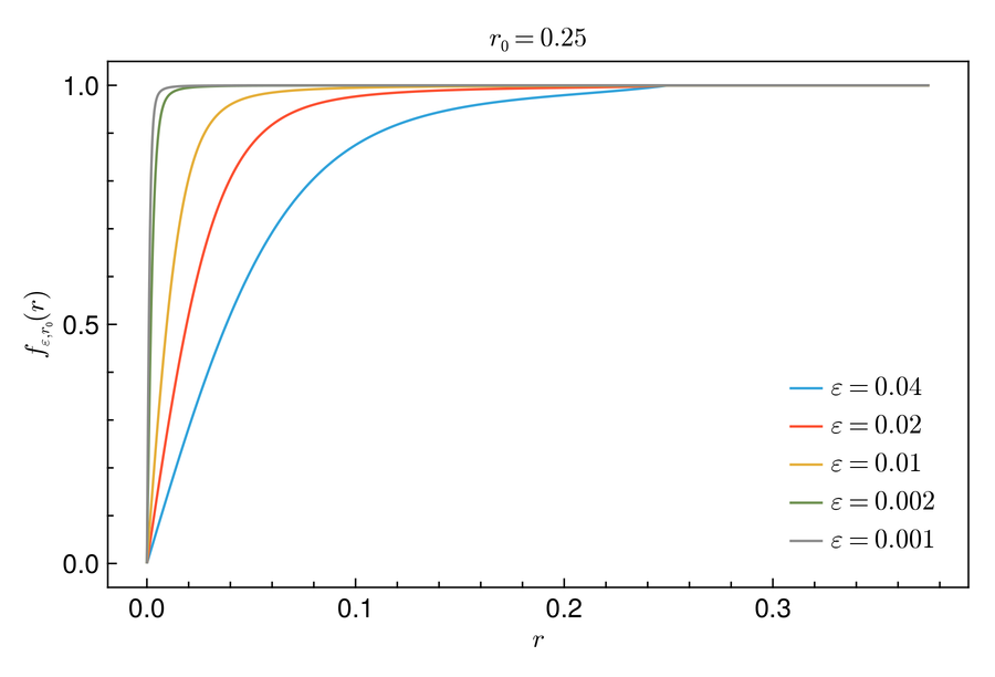
Figure 1. Numerical approximation of $f_{\varepsilon,r_{0}}$.

Starting from the localized approximation $\phi_{\varepsilon}$ of a single vortex, one can then build the following initial condition for (2): given vortex positions $\bm{a}^{0}=(a_{j}^{0})_{j=1,\dots,N}\in\Omega^{*N}$ with degrees $d=(d_{j})_{j=1,\dots,N}\in\left\{\pm 1\right\}^{N}$, we consider

$$\psi_{\varepsilon}^{*}(x;\bm{a}^{0},d)=u^{*}(x;\bm{a}^{0},d)\prod_{j=1}^{N}f_{\varepsilon}(|x-a_{j}^{0}|),\quad x\in\overline{\Omega},$$ (32)

where $u^{*}$ is the canonical harmonic map defined in (13). This numerical strategy can be seen as an operator from the manifold $\{u^{*}(\bm{a},d),\ \bm{a}\in\Omega^{*N},\ d\in\left\{\pm 1\right\}^{N}\}$ to $H^{1}(\Omega,\mathbb{C})$ which smoothes out the canonical harmonic map $u^{*}(\bm{a},d)$ at the singularities locations. Moreover, such initial conditions are also used for instance in [6, 7] and are well-prepared in the sense of Definition 1, as shown in [25, Lemma 14] in the case of Neumann boundary conditions and that we recall here.

Lemma 1 ([25, Lemma 14]).

For any $\bm{a}\in\Omega^{*N}$ and $d\in\left\{\pm 1\right\}^{N}$ and for $r_{0}$ small enough, there exists some constant $C>0$ such that the function $\psi^{*}=\psi_{\varepsilon}^{*}(\bm{a},d)$ constructed above satisfies

$$E_{\varepsilon}(\psi_{\varepsilon}^{*})\leq W_{\varepsilon}(\bm{a},d)+CN\left(\frac{\varepsilon}{r_{0}}\right)^{2}$$ (33)

and

$$\left\|J{\psi_{\varepsilon}^{*}}-\pi\sum_{j=1}^{N}d_{j}\delta_{a_{j}}\right\|_{\dot{{\rm W}}^{-1,1}}\lesssim\varepsilon.$$ (34)

In particular, the assumptions from Definition 1 are satisfied.

We end this section by stating another important property of such well-prepared initial conditions:

Proposition 1.

Let $\psi_{\varepsilon}^{*}(\bm{a},d)$ be as in Lemma 1 for $\bm{a}\in\Omega^{*N}$, $d\in\left\{\pm 1\right\}^{N}$ and $r_{0}$ small enough. Then,

$$\left\|\psi_{\varepsilon}^{*}(\bm{a},d)-u^{*}(\bm{a},d)\right\|_{L^{2}(\Omega,\mathbb{C})}\lesssim\varepsilon.$$ (35)

$$\left\|j\bigr{(}\psi_{\varepsilon}^{*}(\bm{a},d)\bigr{)}-j\bigr{(}u^{*}(\bm{a},d)\bigr{)}\right\|_{L^{p}(\Omega)}\lesssim_{p}\varepsilon^{\frac{2}{p}-1}\quad\mbox{for $1\leq p<2$.}$$ (36)

Proof.

The convergence is a standard result of Ginzburg–Landau theory and a direct consequence of the energy bound (33), see e.g. [30]. Then, the bound on the $L^{2}$ norm of the difference is obtained thanks to the specific structure of $\psi_{\varepsilon}^{*}$. As $\psi_{\varepsilon}^{*}$ coincides with $u^{*}$ outside of the balls $B_{r_{0}(a_{j})}$, we have

$$\int_{\Omega}|\psi_{\varepsilon}^{*}-u^{*}|^{2}=\sum_{j=1}^{N}\int_{B_{r_{0}}(a_{j})}|1-f_{\varepsilon}(\cdot-a_{j})|^{2}=N\int_{B_{r_{0}(0)}}|1-f_{\varepsilon}|^{2}.$$

Recalling that $1\geq f_{\varepsilon}\geq f_{\varepsilon,\infty}$ together with the lower bound $f_{\varepsilon,\infty}(r)\geq\max\left(0,1-c\left(\frac{\varepsilon}{r}\right)^{2}\right)$ (see [35]), we get

$$\int_{\Omega}|\psi_{\varepsilon}^{*}-u^{*}|^{2}\lesssim\int_{0}^{r_{0}}\min\left(1,c^{2}\left(\frac{\varepsilon}{r}\right)^{4}\right)r\mathrm{d}r=\int_{0}^{\varepsilon\sqrt{c}}r\mathrm{d}r+c^{2}\varepsilon^{4}\int_{\varepsilon\sqrt{c}}^{r_{0}}\frac{1}{r^{3}}\mathrm{d}r\lesssim\varepsilon^{2}.$$ (37)

For the supercurrents, we note that, since $|u^{*}|^{2}=1$ and $f_{\varepsilon}$ is real-valued, we find

$$j(\psi_{\varepsilon}^{*})=j(u^{*})\prod_{j=1}^{N}f_{\varepsilon}(|x-a_{j}|)^{2}$$

Thus using that $|j(u^{*})|\lesssim\frac{1}{|x-a_{j}|}$ for $x$ close to $a_{j}$ (which follows from (15)) and the bound $1\geq f_{\varepsilon,\infty}(r)\geq\max\left(0,1-c\left(\frac{\varepsilon}{r}\right)^{2}\right)$, we find

$$\left\|j(\psi_{\varepsilon}^{*})-j(u^{*})\right\|_{L^{p}(\Omega)}^{p} =\sum_{j=1}^{N}\int_{B_{r_{0}}(a_{j})}|j(u^{*})|^{p}\bigr{(}1-f_{\varepsilon}^{2}(|x-a_{j}|)\bigr{)}^{p}\mathrm{d}x$$

$$\lesssim N\int_{0}^{\varepsilon\sqrt{c}}\frac{1}{r^{p}}r\mathrm{d}r+c^{2p}\varepsilon^{2p}\int_{\varepsilon\sqrt{c}}^{r_{0}}\frac{1}{r^{3p}}r\mathrm{d}r\lesssim\varepsilon^{2-p}.$$

∎

3. Numerical simulation of the Hamiltonian dynamics

In the previous section, we recalled the main analytical results on the vortex motion in the singular limit $\varepsilon\to 0$. We also mentioned sufficient conditions for the initial conditions $\psi_{\varepsilon}^{0}$ to be well-prepared, as well as a numerical strategy to build such functions. Now, we focus on the vortex motion itself and we present an efficient numerical method for the numerical simulation of the Hamiltonian dynamics

$$\begin{cases}\dot{a}_{j}(t)=-\frac{1}{\pi}d_{j}\mathbb{J}\nabla_{a_{j}}W({\bm{a}}(t),d),\\ {a}_{j}(0)={a}^{0}_{j},\end{cases}\quad\text{with}\quad\mathbb{J}=\begin{bmatrix}0&1\\ -1&0\end{bmatrix},$$ (38)

for given initial positions $\bm{a}^{0}\in\Omega^{*N}$ and degrees $d\in\left\{\pm 1\right\}^{N}$. Recall that

$$\forall\ (\bm{a},d)\in\Omega^{*N}\times\{\pm 1\}^{N},\quad W(\bm{a},d)=-\pi\sum_{1\leq i\neq j\leq N}d_{i}d_{j}\ln|a_{i}-a_{j}|-\pi\sum_{j=1}^{N}d_{j}R(a_{j};\bm{a},d),$$ (39)

with $R$ the solution to

$$\begin{cases}\displaystyle\Delta R=0\quad\text{in }\Omega,\\ \displaystyle R=-\sum_{j=1}^{N}d_{j}\ln|x-a_{j}|\quad\text{on }\partial\Omega.\end{cases}$$ (40)

The numerical resolution of the ODE (38) requires the evaluation of the gradient $\nabla_{a_{j}}W({\bm{a}}(t),d)$, which can be done using the following identity (see e.g. [6] or [9, Theorem VIII.3] in the case of Dirichlet boundary conditions),

$$\nabla_{a_{j}}W({\bm{a}},d)=-2\pi d_{j}\nabla_{x}\left(R(x;\bm{a},d)+\sum_{k\neq j}^{N}d_{k}\ln|x-a_{k}|\right)\Biggr{|}_{x=a_{j}}.$$

The solution $R$ to (40) being harmonic and the boundary condition being smooth as long as the vortices stay away from the boundary, it makes sense to use harmonic polynomials to solve it with spectral accuracy for a negligible cost. We now detail how to solve (40) at each time step with such a method. For the sake of simplicity, we choose $\Omega$ as the unit disk in $\mathbb{R}^{2}$ but this strategy is easily transposable to other domains.

We define the family $(h_{n})_{n\geq 1}$ of harmonic polynomials as $h_{1}\equiv 1$ and

$$\forall\ m\in\mathbb{N},\ m\geq 1,\ \forall\ (x,y)\in\mathbb{R}^{2},\quad\begin{cases}h_{2m}(x,y)={\mathfrak{R}}\,{(x+\imath y)^{m}},\\ h_{2m+1}(x,y)={\mathfrak{I}}\,{(x+\imath y)^{m}}.\end{cases}$$ (41)

For any integer $n\geq 1$, we have $\Delta h_{n}=0$. Moreover, $h_{1}$ is of degree $0$ and $h_{2m},h_{2m+1}$ are the only two linearly independent harmonic polynomials of degree $m\geq 1$ in two dimensions. In the case where $\Omega$ is the unit disk, the restriction of these polynomials to the boundary $\partial\Omega$ is nothing else than the basis of the Fourier modes for $2\pi$-periodic functions, i.e.

$$\mathcal{X}_{n}\coloneqq{\rm Span}\,\left\{h_{k}|_{\partial\Omega},\ 1\leq k\leq 2n+1\right\}={\rm Span}\,\left\{\partial\Omega\ni z\mapsto z^{k},\ \partial\Omega\ni z\mapsto\overline{z}^{\ell},\ 0\leq k\leq n,\ 1\leq\ell\leq n\right\}.$$

Solving numerically (40) can then be done following these three steps:

1. Choose a maximum degree $n$, and fix it once and for all. Denote by $\mathbb{P}_{n}$ the $L^{2}(\partial\Omega)$-orthogonal projection operator from $L^{2}(\partial\Omega)$ to $\mathcal{X}_{n}$: for any $g\in L^{2}(\partial\Omega)$,

   $$(\mathbb{P}_{n}g)(e^{\\ i\theta})=\sum_{k=-n}^{n}\widehat{g}(k)e^{\imath k\theta},$$

   where

   $$\widehat{g}(k)=\frac{1}{2\pi}\int_{0}^{2\pi}e^{-\imath k\theta}g(e^{\\ i\theta}){\rm d}\theta.$$

2. Compute the Fourier coefficients $(\widehat{g}_{a}(k))_{-n\leq k\leq n}$ of the Dirichlet boundary condition in (40)

   $$[0,2\pi)\ni\theta\mapsto g_{a}(e^{\\ i\theta})\coloneqq-\sum_{j=1}^{N}d_{j}\ln|(\cos\theta,\sin\theta)-a_{j}|$$

   up to order $n$, for instance using a Fast Fourier Transform (FFT).

3. Compute the (approximate) solution $R_{n}$ to (40) as the harmonic expansion of $\mathbb{P}_{n}g_{a}$:

   $$\forall\ r\in[0,1),\ \forall\ \theta\in[0,2\pi),\quad R_{n}(re^{\\ i\theta})=\sum_{k=-n}^{n}r^{|k|}\widehat{g}_{a}(k)e^{\imath k\theta},$$ (42)

   which is still harmonic by linear combination of harmonic functions.

This strategy differs from the one in [6, 7], where the PDE (40) is typically solved with finite differences in the case $\Omega=(-1,1)^{2}$, or with the Fourier pseudo-spectral method in the $\theta$-direction and with the FEM in the $r$-direction when $\Omega$ is the unit disk. Here, we suggest to use the smoothness of the boundary data $g_{a}$ to use a Fourier approximation, which requires only one FFT to obtain an approximate solution to (40). Moreover, the smoothness of the boundary data $g_{a}$ enables to reach spectral accuracy, see Section 5 for more details.

To conclude this section, we provide in Figure 2 first numerical results describing vortex trajectories in the singular limit $\varepsilon\to 0$. The computational domain is the unit disk $\Omega=B_{1}(0)$, with different initial conditions $\bm{a}^{0}$ and $d$ for each case. The ODE (38) is solved with a 4th-order Runge–Kutta method (RK4, see e.g. [22, Chapter II]) with time step $\delta t=10^{-3}$ up to some time $T$. The PDE (40) is solved at each time step using harmonic polynomials up to degree $n=64$, as described above. We consider here eight cases, some of which are directly taken from [7] in order to validate our method. Note that all the trajectories were obtained in a few seconds on a personal laptop, a significant improvement when compared to the computational cost of the complete PDE (2) for small $\varepsilon$.

Case	$N$	$\bm{a}^{0}$	$d$
Case $1$	$2$	$\left((-0.5,0.0),(0.5,0.0)\right)$	$(1,1)$
Case $2$	$2$	$\left((-0.7,0.0),(0.7,0.0)\right)$	$(-1,1)$
Case $3$	$4$	$\left((-0.6,-0.6),(-0.6,0.6),(0.6,0.6),(0.6,-0.6)\right)$	$(1,-1,1,-1)$
Case $4$	$2$	$\left((-0.25,-0.25),(0.25,0.25)\right)$	$(-1,1)$
Case $5$	$3$	$\left((-0.5,0.0),(0.5,0.0),(0.0,0.0)\right)$	$(1,1,1)$
Case $6$	$3$	$\left((-0.5,0.0),(0.5,0.0),(0.0,0.0)\right)$	$(1,1,-1)$
Case $7$	$9$	$\left((x,y)\right)$ for $x,y\in\left\{-0.3,0,0.3\right\}$	$d_{i}=1$ for $i=1,\dots,9$
Case $8$	$9$	$\left((x,y)\right)$ for $x,y\in\left\{-0.3,0,0.3\right\}$	$d_{i}=1$ for $i=1,\dots,9$, $i\neq 5$, $d_{5}=-1$

Table 1. Different settings for the initial conditions of the reduced Hamiltonian dynamics.

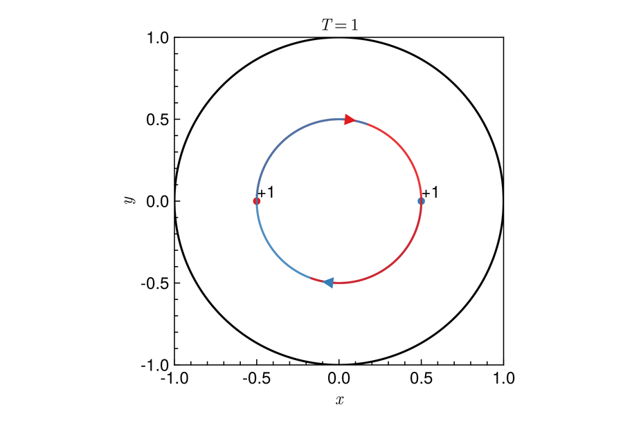
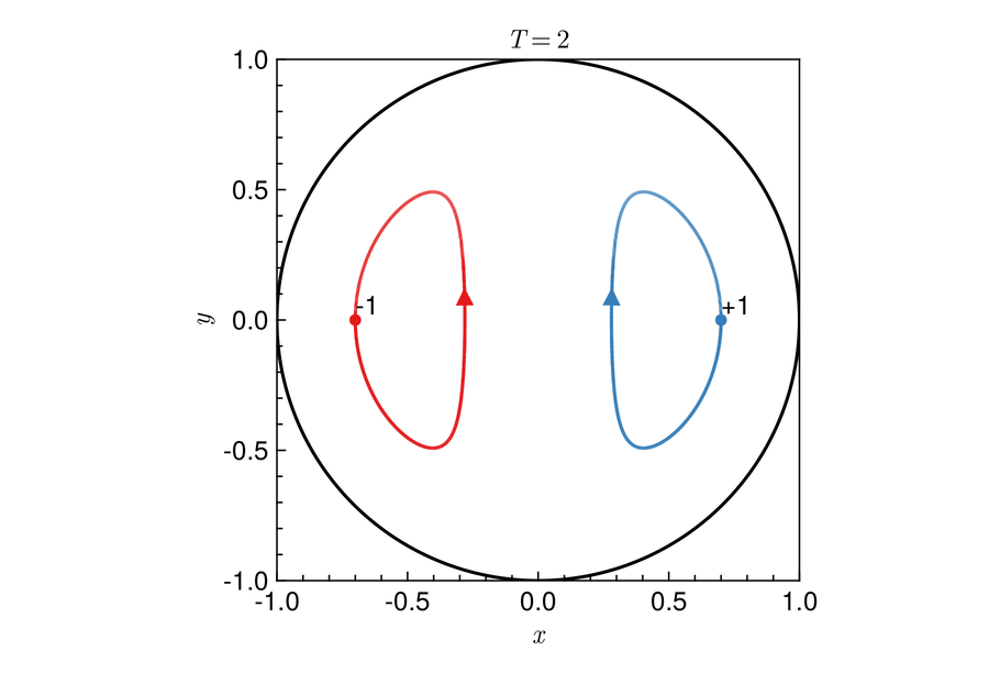
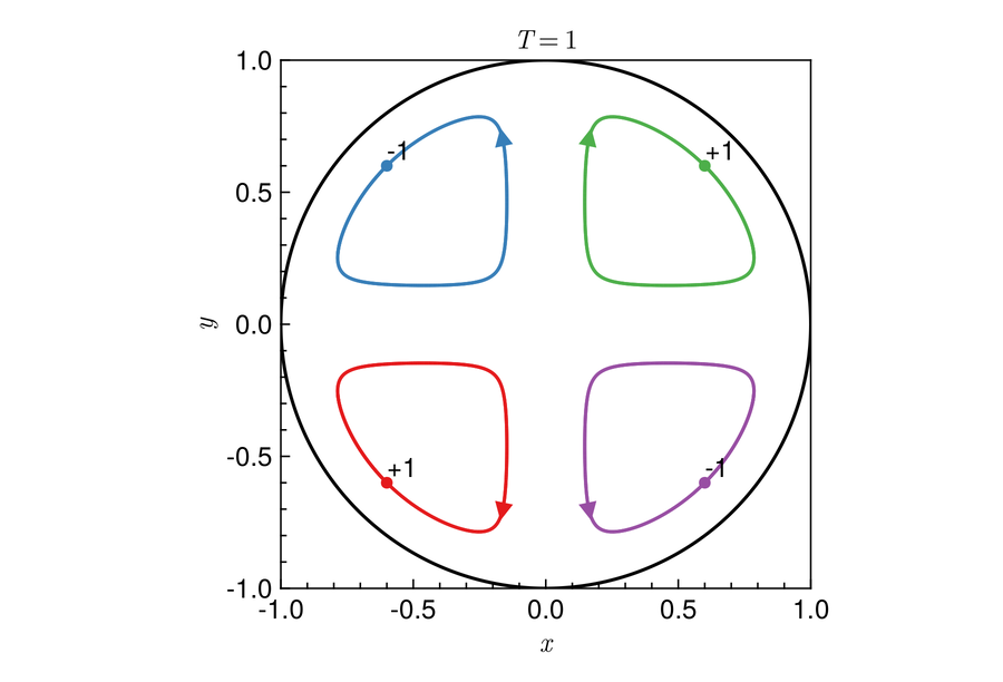
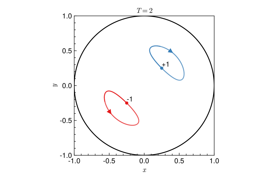
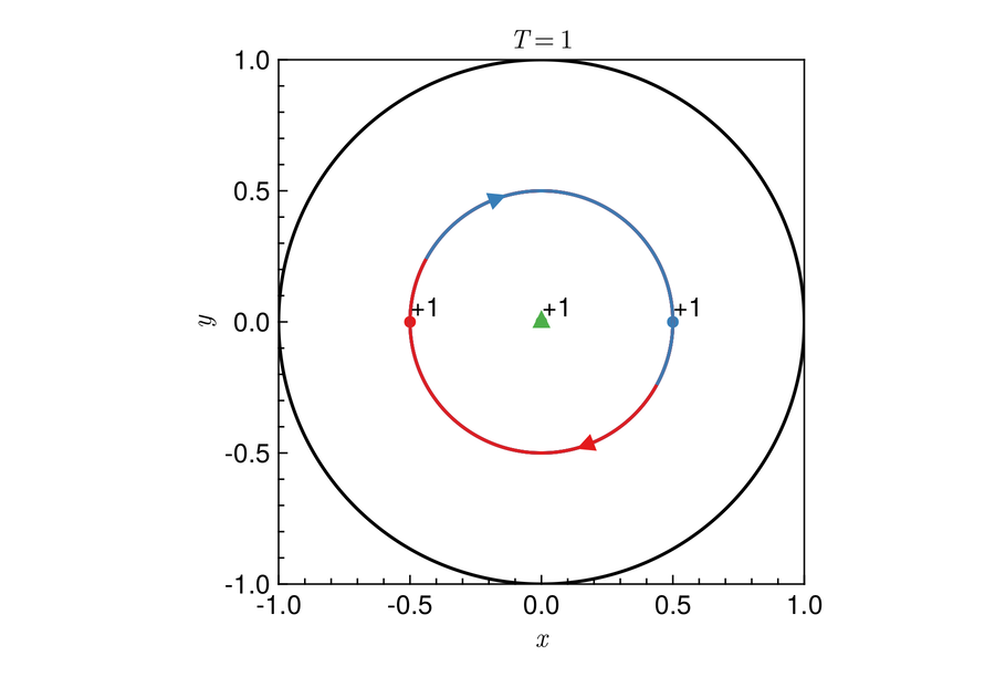
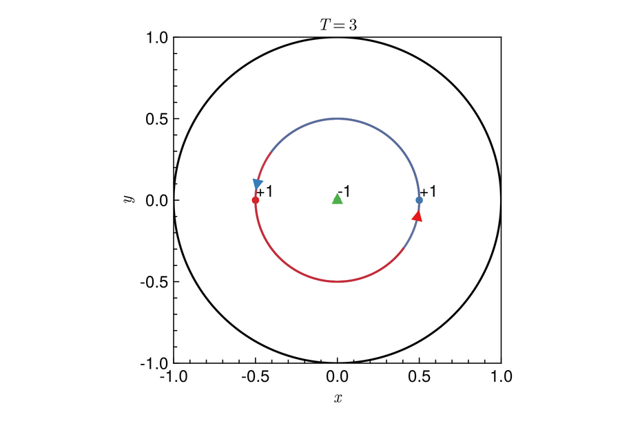
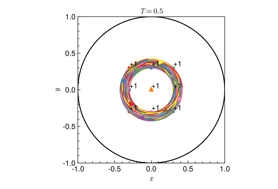
Figure 2. Trajectories of vortices in the singular limit $\varepsilon\to 0$, cases 1 to 8, from left to right and up to bottom. Initial conditions are represented by dots and the different degrees used are specified for each trajectory.

4. Numerical simulation of the Gross–Pitaevskii equation: a new method based on vortex tracking

In this section, we present the main contribution of this paper: a new numerical method for the simulation of (2) in the regime where $\varepsilon>0$ is small but finite. First, we start by describing the method and then we provide some simulations when the initial conditions are given by known vortex positions.

4.1. Description of the method and mathematical justification

Instead of solving directly (2), we propose to take advantage of the well-known behavior in the singular limit $\varepsilon\to 0$ as well as the properties of the smoothing procedure used to obtain well-prepared initial conditions in Section 2.3. This yields the following algorithm:

1. Define initial vortex positions $\bm{a}^{0}\in\Omega^{*N}$ and degrees $d\in\left\{\pm 1\right\}^{N}$. Set up the initial phase $H$ such that the initial condition $\psi_{\varepsilon}^{0}$ from Lemma 1 satisfies homogeneous Neumann boundary conditions. Compute and store the radial function $f_{\varepsilon}$.

2. Evolve $\bm{a}(t)$ according to the ODE (38) up to some maximum time $T$.

3. At time $t>0$, build back an approximation of the wave function from the vortex positions ${\bm{a}}(t)$ as

   $$\psi_{\varepsilon}^{*}(t)=\psi_{\varepsilon}^{*}({\bm{a}}(t),d)=u^{*}(\cdot;{\bm{a}}(t),d)\prod_{j=1}^{N}f_{\varepsilon}(|\cdot-a_{j}(t)|)\quad x\in\overline{\Omega},$$ (43)

   where $u^{*}(x;{\bm{a}}(t),d)$ is the canonical harmonic map defined by

   $$u^{*}(x;{\bm{a}}(t),d)=\exp\left(\imath H(x)\right)\prod_{j=1}^{N}\left(\frac{x-a_{j}}{|x-a_{j}|}\right)^{d_{j}},$$ (44)

   with $H$ the unique zero-mean harmonic function solving

   $$\begin{cases}\Delta H=0\quad\text{in }\Omega,\\ \displaystyle\partial_{\nu}H(x)=-\sum_{j=1}^{N}d_{j}\partial_{\nu}\theta(x-a_{j})=\sum_{j=1}^{N}d_{j}\partial_{\tau}\ln|x-a_{j}|\quad\text{on }\partial\Omega.\end{cases}$$ (45)

   Computing $H$ with the appropriate boundary conditions is required so that the approximate solution $\psi_{\varepsilon}^{*}(t)$ satisfies homogeneous Neumann boundary conditions. This Laplace’s equation can be solved using the same harmonic polynomial basis than the one used to solve (40). However, note that the harmonic function $H$ is defined only up to a constant: this implies that the reconstructed wave function $\psi_{\varepsilon}^{*}$ is an approximation of $\psi_{\varepsilon}$ only up to a constant phase. However, when looking at quantity of interest such as the supercurrents or the vorticity, this phase factor has no influence.

The method we propose can be summarized by the diagram in Figure 3.

initial conditions $(\bm{a}^{0},d)\in\Omega^{*N}\times\left\{\pm 1\right\}^{N}$	$\xrightarrow[\text{ODE}]{\text{evolve}}$	$({\bm{a}}(t),d)\in\Omega^{*N}\times\left\{\pm 1\right\}^{N}$
$\downarrow$ smoothing		smoothing $\downarrow$
well-prepared wave function $\psi_{\varepsilon}^{0}=\psi_{\varepsilon}^{*}(\bm{a}^{0},d)$	$\xrightarrow[\text{GP}]{\text{evolve}}$	$\psi_{\varepsilon}(t)\approx\psi_{\varepsilon}^{*}({\bm{a}}(t),d)$	(up to a constant phase)

Figure 3. Diagram summarizing the numerical simulation of the GP equation (2) via vortex tracking.

One can then observe that, the smaller $\varepsilon$, the more commutative the diagram from Figure 3 is. Mathematically, the justification of our method is a simple combination of the results we recalled in Section 2, that we present here in three points.

Proposition 2.

Let $\bm{a}^{0}\in\Omega^{*N}$ and $d\in\left\{\pm 1\right\}^{N}$ be given as initial data. Let ${\bm{a}}(t)$ evolves according to (38). Let $\psi_{\varepsilon}$ be the solution to the GP equation (2) with initial conditions $\psi_{\varepsilon}^{0}=\psi_{\varepsilon}(\bm{a}^{0})$ for $\varepsilon$ and $r_{0}$ small enough. Then, for all $0\leq t\leq\tau_{\varepsilon,\bm{a}^{0}}$,

1. Both $\psi_{\varepsilon}(t)$ and $\psi_{\varepsilon}^{*}(t)$ are close to be energetically optimal:

   $$E_{\varepsilon}(\psi_{\varepsilon}(t)),E_{\varepsilon}(\psi_{\varepsilon}^{*}(t))\leq W_{\varepsilon}({\bm{a}}(t),d)+C\varepsilon^{\frac{1}{2}}.$$

2. Up to a constant phase, the error $\left\|\psi_{\varepsilon}(t)-\psi_{\varepsilon}^{*}(t)\right\|_{L^{2}}$ goes to $0$ as $\varepsilon\to 0$.

3. The Jacobians and supercurrents of $\psi_{\varepsilon}$ and $\psi_{\varepsilon}^{*}$ are close, in the sense

   $$\left\|J\psi_{\varepsilon}(t)-J\psi_{\varepsilon}^{*}(t)\right\|_{\dot{\rm W}^{-1,1}}\lesssim\varepsilon^{\beta}\quad\text{and}\quad\left\|j(\psi_{\varepsilon}(t))-j(\psi_{\varepsilon}^{*}(t))\right\|_{L^{\frac{4}{3}}}\lesssim\varepsilon^{\gamma}.$$

Here, $\beta$, $\gamma\leq\frac{1}{2}$ and $\tau_{\varepsilon,\bm{a}^{0}}$ are defined in Theorem 1.

Proof.

These properties are all consequences of the general fact that, if the initial conditions are well-prepared in the sense of Definition 1, then well-preparedness is conserved along time. In particular,

(1) is a direct consequence of the conservation of energy for (2) and Hamiltonian systems as well as the bound (33) satisfied by the smoothed canonical harmonic maps.

(2) is obtained after recalling that both $\psi_{\varepsilon}(t)$ and $\psi_{\varepsilon}^{*}(t)$ converge towards $u^{*}({\bm{a}}(t),d)$ in $L^{2}(\Omega)$ up to a constant phase (see (25) and Proposition 1).

(3) is the triangular inequality applied to (28) and (34) for the Jacobian and to (28) and (36) for the supercurrents, the bound $\gamma\leq\frac{1}{2}$ coming from (36). ∎

At this point, some comments have to be made. First, the smaller epsilon, the more accurate is the approximation $\psi_{\varepsilon}^{*}$. This is a clear improvement with respect to standard techniques used to solve numerically nonlinear Schrödinger type equations such as those mentioned in the introduction, where very small values of $\varepsilon$ requires very fine discretization in both space and time to ensure numerical stability. Here, $\varepsilon$ only intervenes through the numerical resolution of the nonlinear ODE (30) which is only one dimensional, and thus easily approximated with high accuracy. Moreover, this step only has to be done once at the beginning of the simulation as the function $f_{\varepsilon}$ used to build the approximation $\psi_{\varepsilon}$ is time-independent and can be saved for the whole simulation. Of course, such an improvement is only possible thanks to the well-known analytical theory of the singular limit $\varepsilon\to 0$ presented in the beginning of this paper. Second, there is, up to our knowledge, no available quantitative bounds on the error $\left\|\psi_{\varepsilon}(t)-u^{*}({\bm{a}}(t),d)\right\|_{L^{2}}$ in the limit $\varepsilon\to 0$ as most of the asymptotic results are based on compactness arguments. The only quantitative bounds available in the literature are the refined Jacobian estimates derived in [25], but these are bounds in weak norms that are not computable numerically. However, in the same paper, the authors also derived bounds on the $L^{p}$ norms of the supercurrents for $p<2$, which can be exploited to evaluate numerically the accuracy of our method, see Section 5. Finally, note that the asymptotic dynamics of the vortices is only valid as long as the vortices stay away from each other and from the boundary, a condition traduced by the requirement of $r_{0}$ being small enough for the initial condition to be well-prepared and to reconstruct the wave function without any overlap between the vortices. In particular, nonlinear physical phenomena triggered by overlapping vortices (or vortices too close to the boundary), such as the radiations and sound waves observed numerically in [7], cannot be produced with our method. However, a possible improvement could be to use the vortex-tracking method up to some time $t$ where the vortices become close enough to each other and then switch to a standard PDE solver to simulate the vortex interaction.

4.2. Vortex positions as initial conditions

We now present some numerical simulations of approximate solutions to (2) in the regime of small $\varepsilon$. The reference vortex trajectories are those from Section 3. The solution of (30) is approximated numerically using 1D finite elements with small mesh size $\delta r=10^{-5}$ and $r_{0}=0.1$. Finally, the solution to Laplace’s equation (45) in the smoothing process at time $t>0$ is computed using harmonic polynomials of degree $n=64$. Here, the initial vortex positions $\bm{a}^{0}$ are provided as input data and we present the numerical results obtained by the application of our numerical method to cases 1, 2, 3 and 6 from Section 3, for $\varepsilon=10^{-2}$. Moreover, note that the phases displayed in Figures 4–7 are those of the canonical harmonic map $u^{*}(\bm{a}(t),d)$ when far from the vortices.

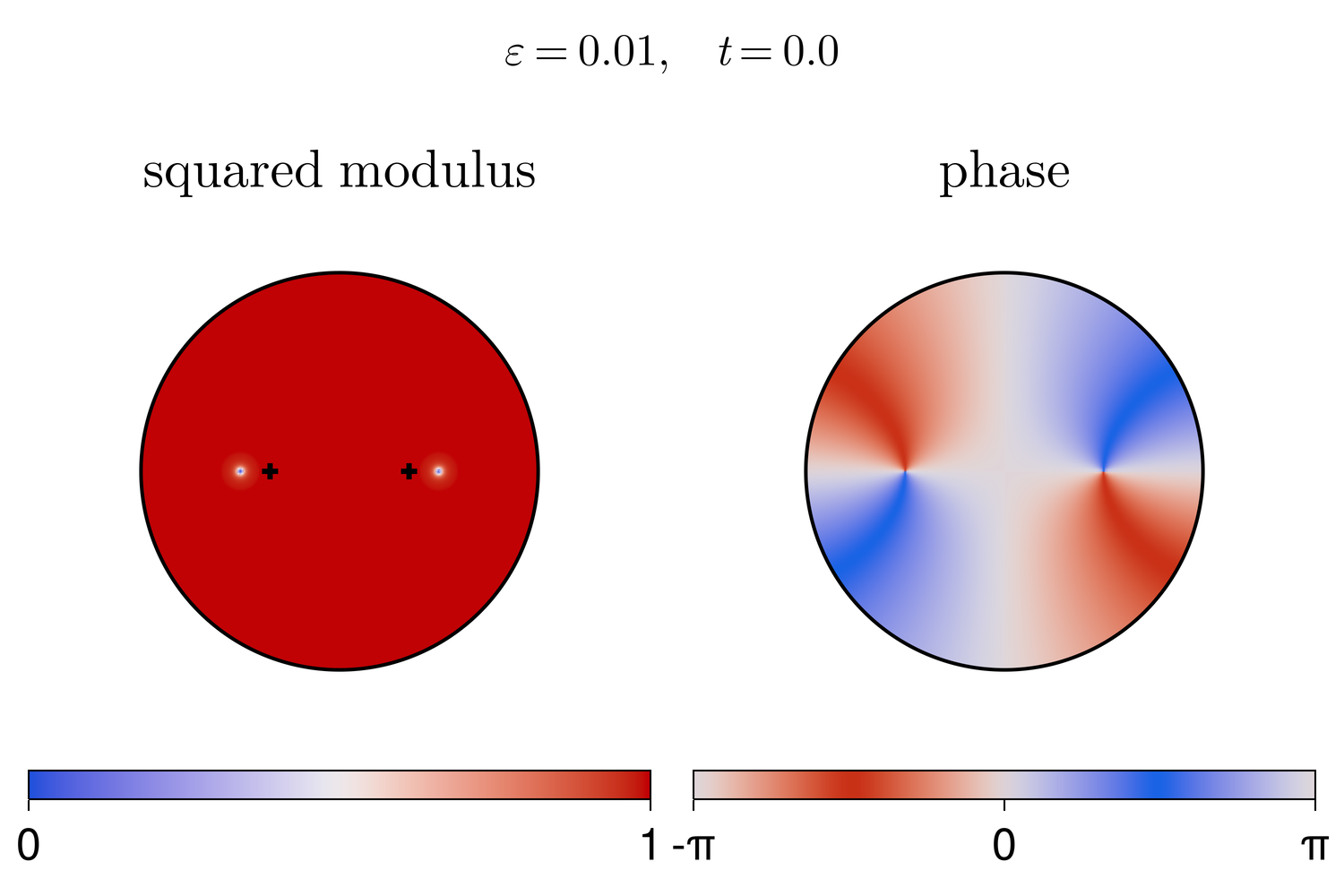
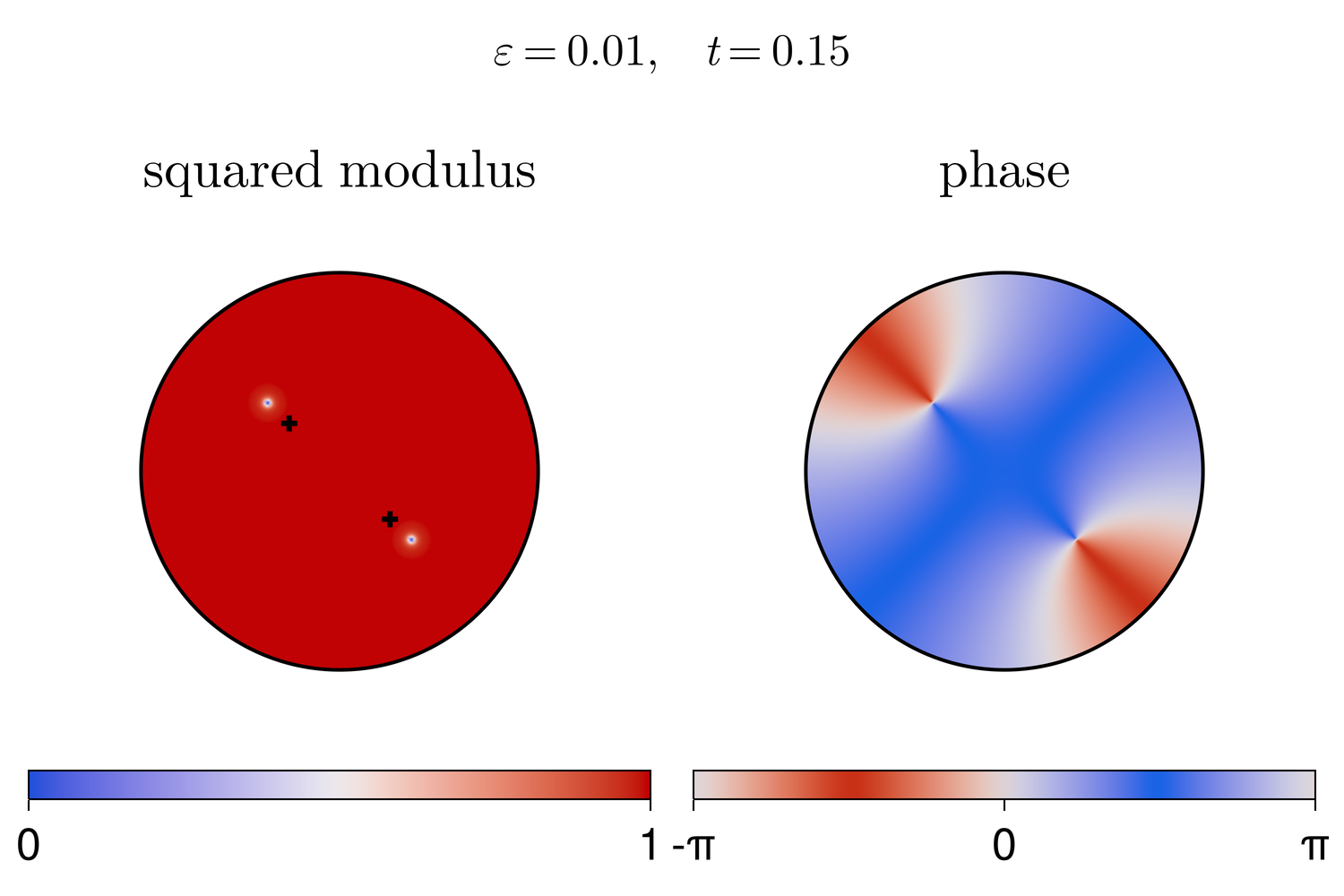
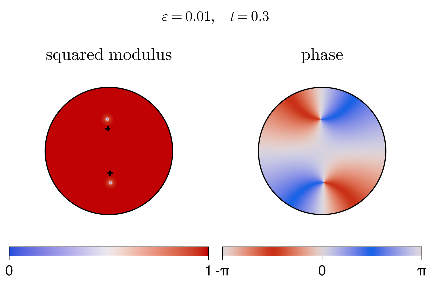
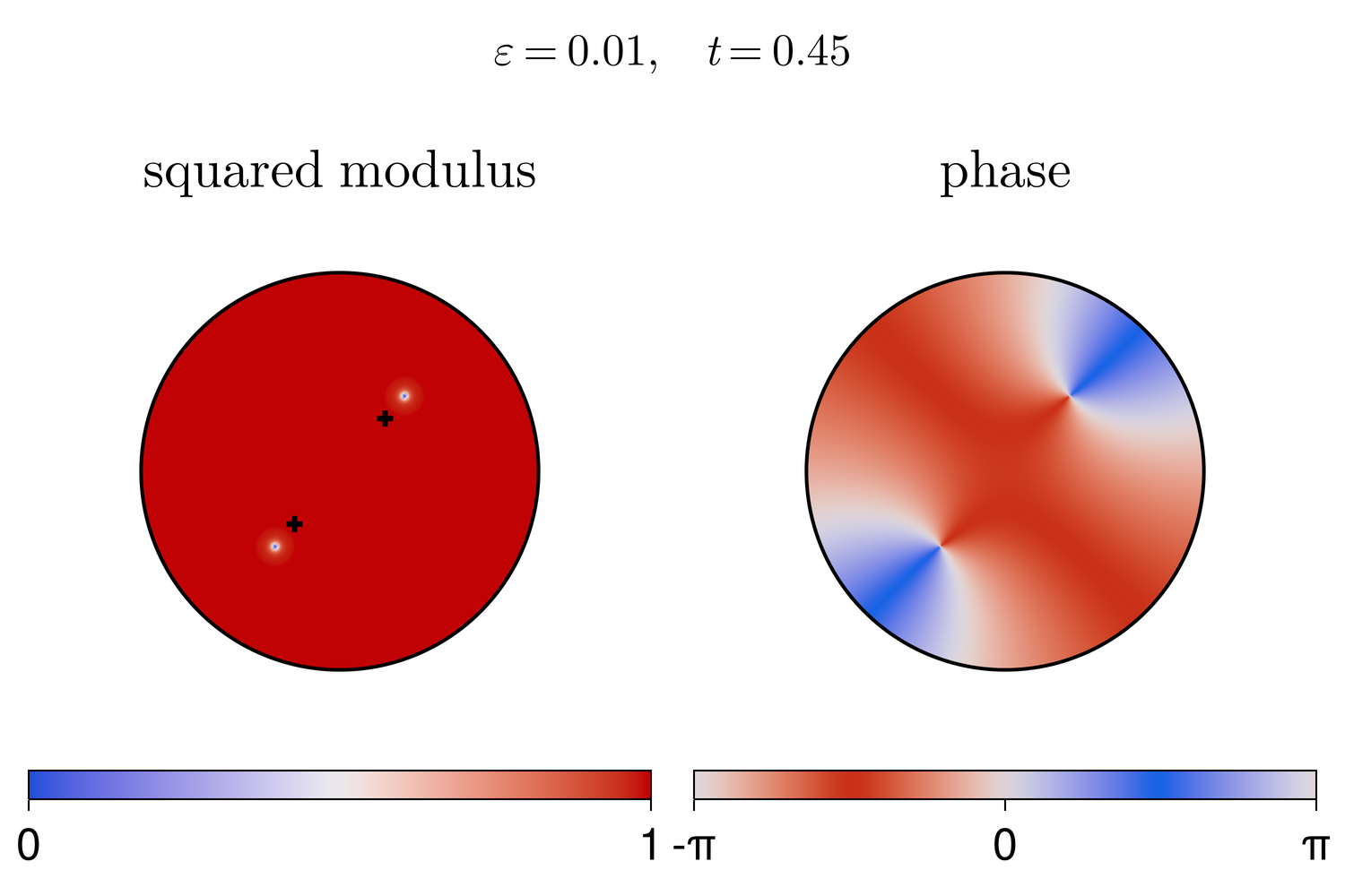
Figure 4. Case 1: Squared modulus and phase of $\psi_{\varepsilon}^{*}(t)$ for different times $t$.

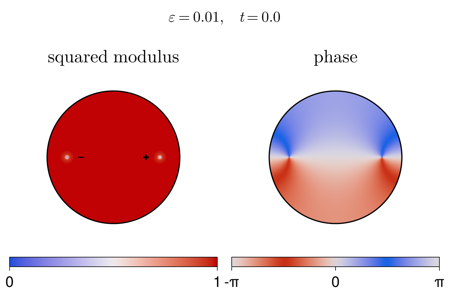
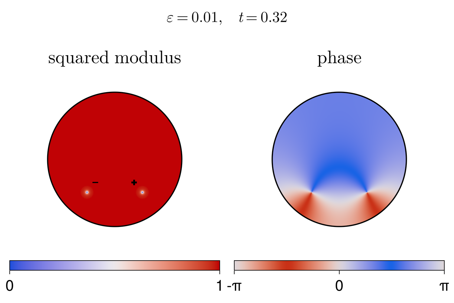
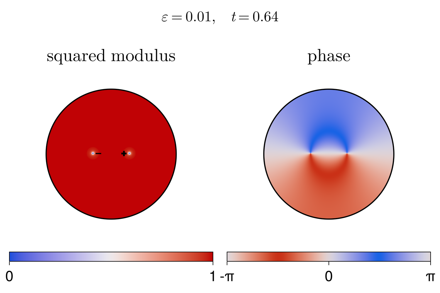
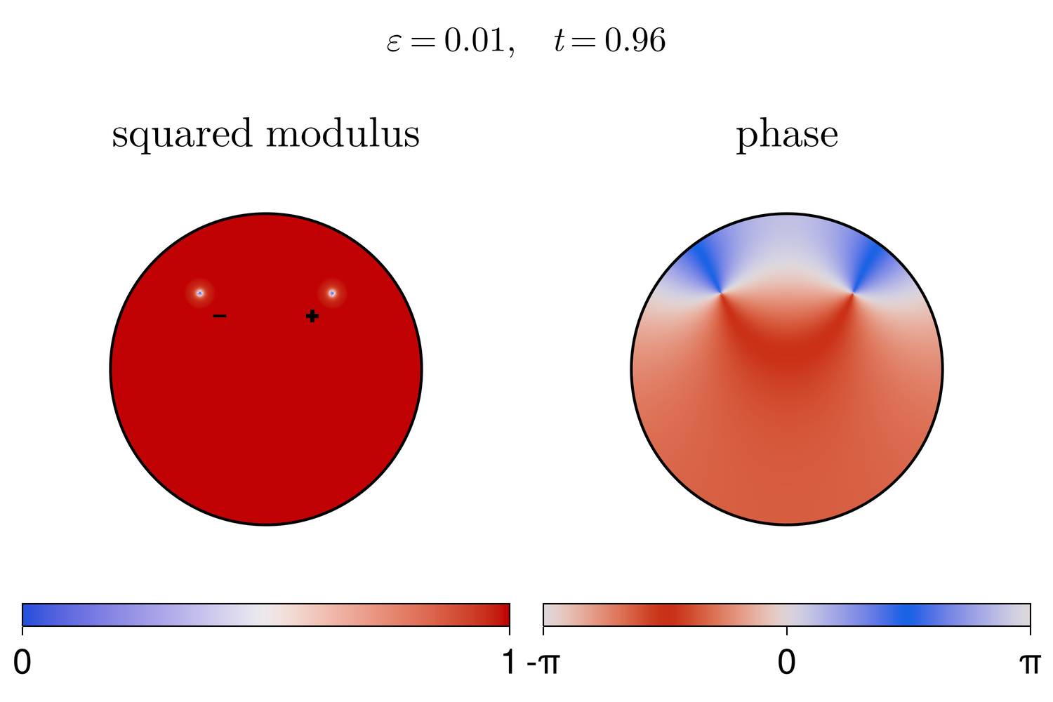
Figure 5. Case 2: Squared modulus and phase of $\psi_{\varepsilon}^{*}(t)$ for different times $t$.

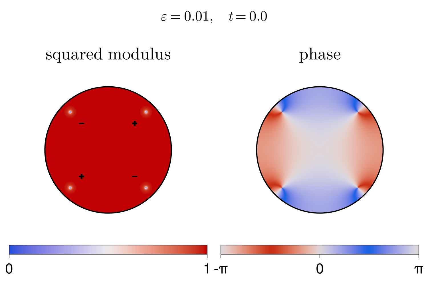
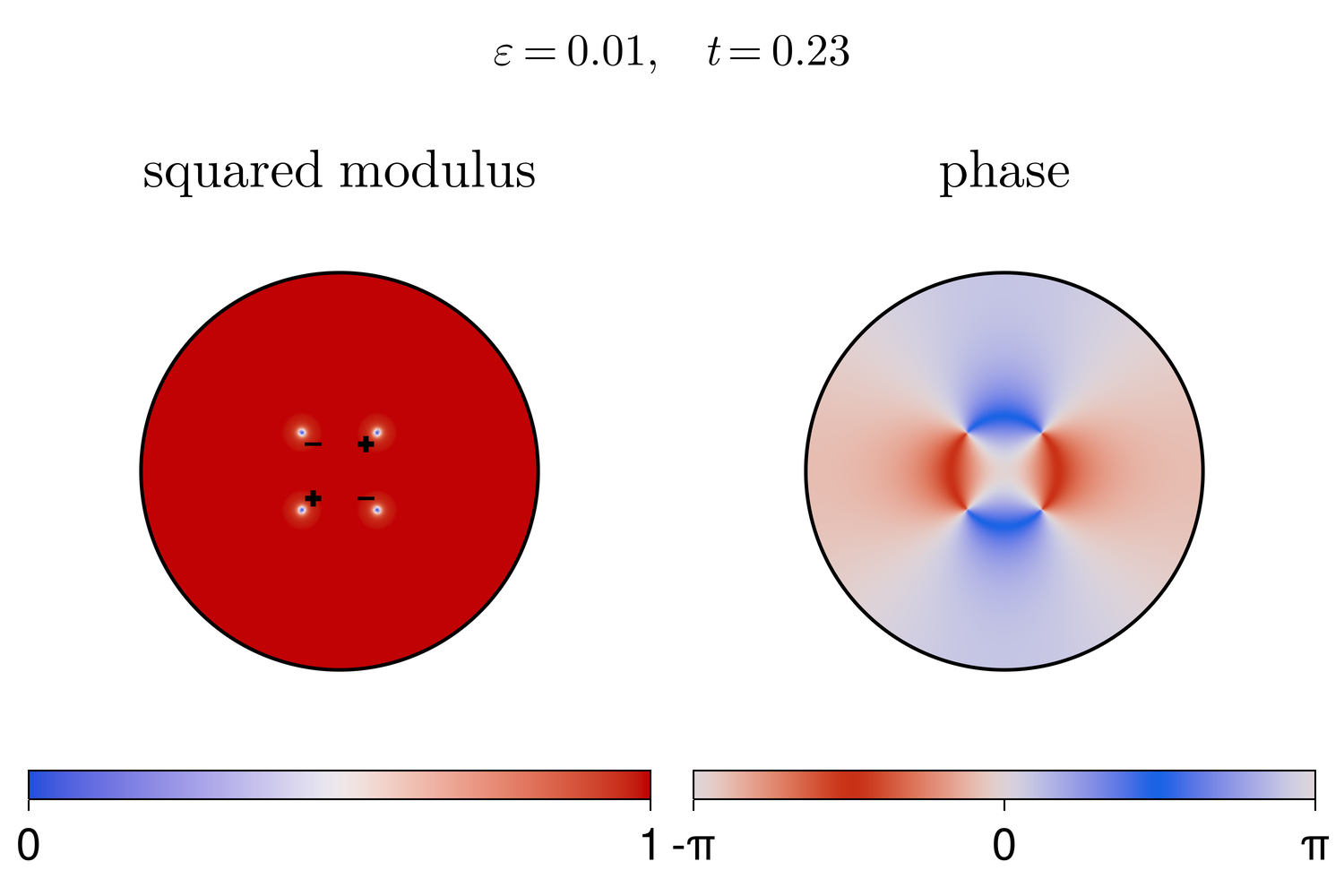
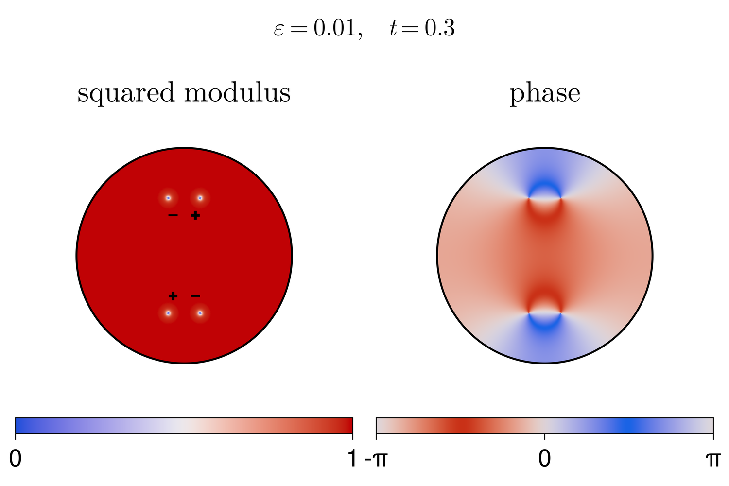
Figure 6. Case 3: Squared modulus and phase of $\psi_{\varepsilon}^{*}(t)$ for different times $t$.

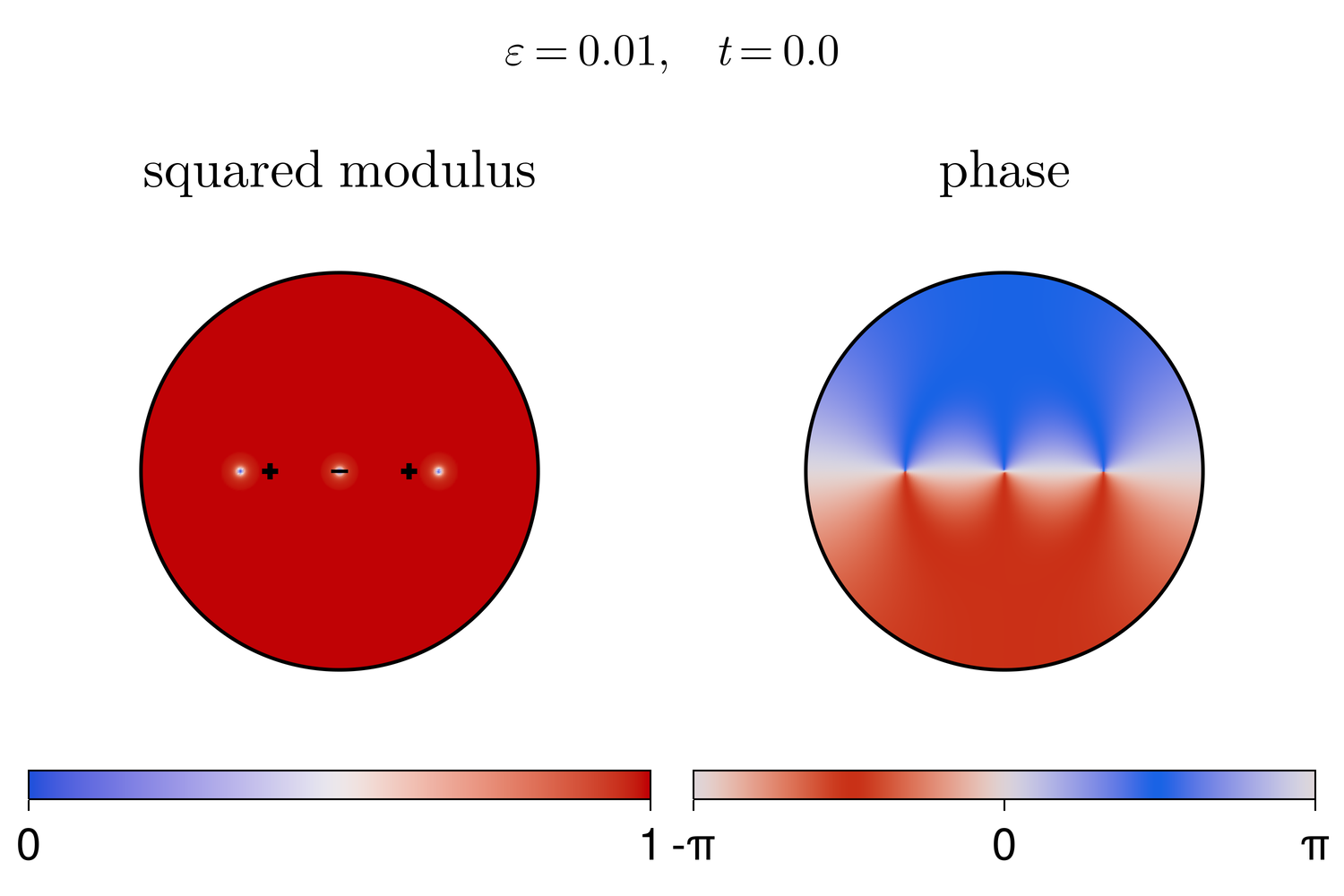
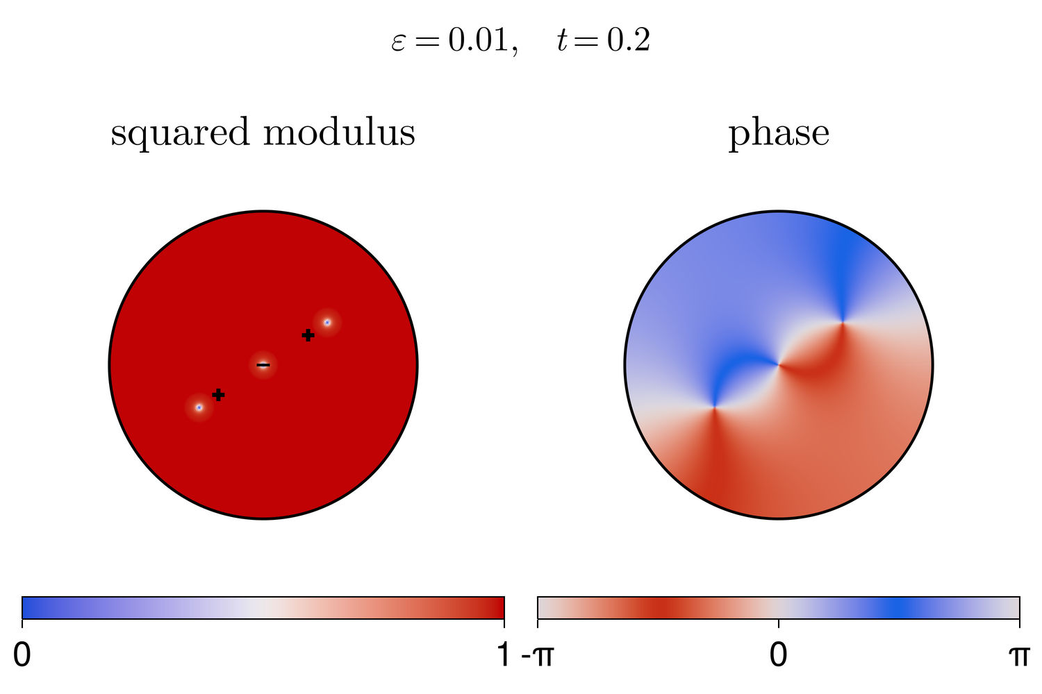
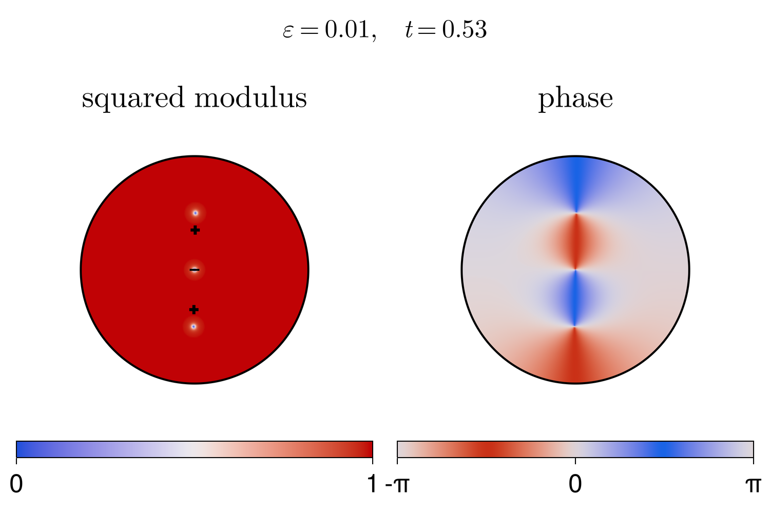
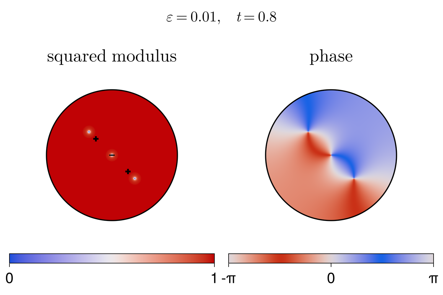
Figure 7. Case 6: Squared modulus and phase of $\psi_{\varepsilon}^{*}(t)$ for different times $t$.

5. Error control on the supercurrents

We focus in this section on providing error estimates on the supercurrents in the $L^{\frac{4}{3}}$ norm from Theorem 1. Precisely, we bound the error between the supercurrents of the exact solution of (2) and the approximated solution obtained with our method in terms of the parameter $\varepsilon$ and the two discretization parameters, i.e. the time step $\delta t$ and the number of harmonic polynomials $n$.

To this end, let us denote by $\{\bm{b}(t)\}_{t\in\delta t\mathbb{N}}$ the approximated trajectory for the Hamiltonian dynamics (38) obtained via a RK4 ODE solver with time step $\delta t$ and $n$ harmonic polynomials in the numerical resolution of the PDE (40) at each time step. More precisely, $\{b(t)\}_{t\in\delta t\mathbb{N}}$ is the numerical solution of

$$\begin{cases}\dot{\bm{b}}(t)=F^{n}(\bm{b}(t)),\\ \bm{b}(0)=\bm{b}^{0},\end{cases}$$ (46)

where the approximate forcing term $F^{n}=(F^{n}_{1},...,F^{n}_{N}):\Omega^{N}\rightarrow\mathbb{R}$ we evaluate at each time step is given by

$$F_{j}^{n}(\bm{b})=2\mathbb{J}\biggr{(}\nabla_{x}R_{n}(x;\bm{b},d)\bigr{\rvert}_{x=b_{j}}+\sum_{k\neq j}^{N}d_{k}\frac{b_{j}-b_{k}}{|b_{j}-b_{k}|}\biggr{)}\quad\quad\mbox{for some }\{d_{j}\}_{j=1}^{N}\in\{\pm 1\}^{N},$$

with $R_{n}(\cdot;\bm{b},d):\Omega\rightarrow\mathbb{R}$ being the solution of

$$\begin{cases}\Delta_{x}R_{n}(x;\bm{b},d)=0,\quad\text{in }\Omega,\\ \displaystyle R_{n}(x;\bm{b},d)=-\mathbb{P}_{n}\biggr{(}\sum_{j=1}^{N}d_{j}\log|x-b_{j}|\biggr{)},\quad\text{on }\partial\Omega,\end{cases}$$

where $\mathbb{P}_{n}$ is the $L^{2}(\partial\Omega)$-orthogonal projection on the bases of harmonic polynomials up to order $n$ on the boundary. Then using harmonic polynomials up to degree $n$ to approximate the function $H$ in (45), the reconstructed wave-function at time $t\in\delta t\mathbb{N}$ is given by

$$\psi_{\varepsilon}^{*}(t)=\psi_{\varepsilon}^{*}(\bm{b}(t),d)=\exp\left(\imath H_{n}\right)\prod_{j=1}^{N}f_{\varepsilon}(|\cdot-b_{j}(t)|)\left(\frac{\cdot-b_{j}(t)}{|\cdot-b_{j}(t)|}\right)^{d_{j}}\quad x\in\overline{\Omega},$$ (47)

where $b_{j}(t)\in\Omega$ denotes the $j^{\rm th}$ component of $\bm{b}(t)$, and $H_{n}$ is the unique zero-mean harmonic function satisfying

$$\begin{cases}\Delta H_{n}=0\quad\text{in }\Omega,\\ \displaystyle\partial_{\nu}H_{n}(x)=\mathbb{P}_{n}\biggr{(}\sum_{j=1}^{N}d_{j}\partial_{\tau}\ln|x-b_{j}(t)|\biggr{)},\quad\text{on }\partial\Omega.\end{cases}$$ (48)

Let us also denote by $\{\bm{a}(t)\}_{t\geq 0}$ the exact solution of the Hamiltonian dynamics (38). Then the first result of this section is an estimate on the distance $|\bm{a}(t)-\bm{b}(t)|$ in terms of the discretization parameters $\delta t$ and $n$.

Lemma 2 (Error estimate on Hamiltonian dynamics).

Let $\Omega\subset\mathbb{R}^{2}$ be the unit disk, let $\{\bm{a}(t)\}_{t\geq 0}$ denote the exact solution to the Hamiltonian dynamics (38) with initial condition $\bm{a}^{0}=(a_{j}^{0})_{j=1,\dots,N}$ and degrees $(d_{j})_{j=1,\dots,N}$. Let $\bm{b}(t)$ be the approximated ODE trajectory with the same degrees and initial position $\bm{b}^{0}=(b_{j}^{0})_{j=1,\dots N}$, with harmonic polynomials of degree up to $n$ and time step $\delta t$. Suppose that, for some $T>0$,

$$\rho_{T}=\min_{t\leq T}\min_{j\neq k}\{|b_{j}(t)-b_{k}(t)|,\mathrm{dist}(b_{k}(t),\partial\Omega),|a_{j}(t)-a_{k}(t)|,\mathrm{dist}(a_{j}(t),\partial\Omega)\}>0.$$

Then we have

$$|\bm{a}(t)-\bm{b}(t)|\lesssim_{\ell,T}\biggr{(}|\bm{a}^{0}-\bm{b}^{0}|+(1-\rho_{T})^{n}n^{1-\ell}\biggr{)}+\delta t^{4}\quad\mbox{for any $t\in\{k\delta t\}_{k\in\mathbb{N}}$ with $t\leq T$}$$ (49)

for any $\ell\in\mathbb{N}$, where the implicit constant depends on $\ell\in\mathbb{N}$ and $T>0$ but is independent of $\bm{a}^{0},\bm{b}^{0},n,\delta t$ and $t$.

Proof.

The proof is immediate from the triangle inequality and Lemmas 5 and Lemma 6 in the appendix. ∎

Combining the above lemma with the previous results, we can now estimate the error between the supercurrents of the reconstructed solution in (47) and the exact solution of the Gross–Pitaevskii equation (2).

Theorem 2 (Error estimate on supercurrents).

Let $\Omega\subset\mathbb{R}^{2}$ be the unit disk, and $\{\psi_{\varepsilon}(t)\}_{\varepsilon<\varepsilon_{0}}$ be the solution of (2) with well-prepared initial conditions, in the sense of Definition 1 for some initial vortices with positions $\bm{a}^{0}=(a_{j}^{0})_{j=1,\dots,N}$ and degrees $(d_{j})_{j=1,\dots,N}$. Let $\bm{b}(t)$ be the approximated ODE trajectory with the same degrees and initial position $\bm{b}^{0}=(b_{j}^{0})_{j=1,\dots N}$, with harmonic polynomials of degree up to $n$ and time step $\delta t$. Let $\psi^{*}_{\varepsilon}(t)$ be the reconstructed wave function described above. Suppose that, for some $T>0$,

$$\rho_{T}=\min_{t\leq T}\min\{|b_{j}(t)-b_{k}(t)|,\mathrm{dist}(b_{k}(t),\partial\Omega),|a_{j}(t)-a_{k}(t)|,\mathrm{dist}(a_{j}(t),\partial\Omega):j\neq k\}$$

is such that $0<\rho_{T}<1$. Then we have

$$\left\|j\bigr{(}\psi^{*}_{\varepsilon}(t)\bigr{)}-j\bigr{(}\psi_{\varepsilon}(t)\bigr{)}\right\|_{L^{\frac{4}{3}}(\Omega)}\lesssim_{\ell,T}\varepsilon^{\gamma}+n^{-\ell+\frac{1}{2}}+\sqrt{|\bm{a}^{0}-\bm{b}^{0}|+(1-\rho_{T})^{n}n^{1-\ell}+\delta t^{4}},$$ (50)

for any $t\in[0,T]$ and $\ell\in\mathbb{N}$, where $0<\gamma\leq\frac{1}{2}$ and the implicit constant depends on $\ell$ and $T>0$ but is independent of $\bm{a}^{0}$, $\bm{b}^{0}$, $\varepsilon,n$, and $\delta t$.

Proof.

Throughout this proof we use various classical estimates, whose proofs are compiled in the appendix for the sake of presentation. At any time we can split the error into

$$\begin{split}\left\|j(\psi_{\varepsilon}(t))-j(\psi_{\varepsilon}^{*}(t))\right\|_{L^{\frac{4}{3}}}&\leq\left\|j(\psi_{\varepsilon}(t))-j(u^{*}(\bm{a}(t),d))\right\|_{L^{\frac{4}{3}}}\\ &+\left\|j\bigr{(}u^{*}(\bm{a}(t),d)\bigr{)}-j\bigr{(}u^{*}(\bm{b}(t),d)\bigr{)}\right\|_{L^{\frac{4}{3}}}\\ &+\left\|j\bigr{(}u^{*}(\bm{b}(t),d)\bigr{)}-j(\psi_{\varepsilon}^{*}(t))\right\|_{L^{\frac{4}{3}}},\end{split}$$ (51)

where $\bm{a}(t)$ denotes the exact Hamiltonian trajectory of the vortices given by the solution of eq. (24). By Theorem 1, the first term is bounded by $\lesssim\varepsilon^{\gamma}$ for some $0<\gamma<1$, which yields the first term in (50).

The second term can be bounded using (15) and combining estimates (67) and (75) in the appendix to obtain

$$\left\|j\bigr{(}u^{*}(\bm{a}(t),d)\bigr{)}-j\bigr{(}u^{*}(\bm{b}(t),d)\bigr{)}\right\|_{L^{\frac{4}{3}}} =\left\|\nabla G(x;\bm{a}(t),d)-\nabla G(x;\bm{b}(t),d)\right\|_{L^{\frac{4}{3}}}$$

$$\lesssim_{\rho_{T}}{|\bm{a}(t)-\bm{b}(t)|}+{|\bm{a}(t)-\bm{b}(t)|}^{\frac{1}{2}},$$

where the constants depend on $\rho_{T}$. Thus, by estimate (74) in Lemma 5 and Lemma 6 we find

$$\left\|j\bigr{(}u^{*}(\bm{a}(t),d)\bigr{)}-j\bigr{(}u^{*}(\bm{b}(t),d)\bigr{)}\right\|_{L^{\frac{4}{3}}} \lesssim_{\ell,T}\sqrt{\biggr{(}|\bm{a^{0}}-\bm{b^{0}}|+\frac{(1-\rho_{T})^{n}n^{1-\ell}}{\rho_{T}^{1+\ell}}T\biggr{)}e^{Ct/\rho_{T}^{5/2}}+\delta t^{4}},$$ (52)

$$\lesssim_{\ell,T}\sqrt{|\bm{a^{0}}-\bm{b^{0}}|+(1-\rho_{T})^{n}n^{1-\ell}+\delta t^{4}}.$$ (53)

where the implicit constant depends on $\ell\in\mathbb{N}$ and $T>0$ but is independent of $\bm{a}^{0},\bm{b}^{0},\delta t$ and $n$. This yields the last term in (50).

To bound the third term, notice that the reconstructed wave function $\psi_{\varepsilon}^{*}$ is obtained after an additional approximation in the resolution of Laplace’s equation (45) that defines the phase factor $H$. Therefore, by the triangle inequality we find

$$\left\|j\bigr{(}u^{*}(\bm{b}(t),d)\bigr{)}-j(\psi_{\varepsilon}^{*}(t))\right\|_{L^{\frac{4}{3}}} \leq\left\|j\bigr{(}u^{*}(\bm{b}(t),d)\bigr{)}-j\bigr{(}u_{n}^{*}(\bm{b}(t),d)\bigr{)}\right\|_{L^{\frac{4}{3}}}+\left\|j\bigr{(}u_{n}^{*}(\bm{b}(t),d)\bigr{)}-j\bigr{(}\psi_{\varepsilon}^{*}(t)\bigr{)}\right\|_{L^{\frac{4}{3}}},$$

where $u^{*}_{n}(\bm{b}(t),d)$ is the approximated canonical harmonic map

$$u_{n}^{*}(\bm{b}(t),d)=\exp\left(\imath H_{n}\right)\prod_{j=1}^{N}\left(\frac{\cdot-b_{j}(t)}{|\cdot-b_{j}(t)|}\right)^{d_{j}}\quad\mbox{with $H_{n}$ defined in \eqref{eq:H_rebuilt_n}.}$$

Since $u_{n}^{*}(\bm{b}(t),d)$ and $u^{*}(\bm{b}(t),d)$ have the same singularities, from Hölder’s inequality we have

$$\left\|j\bigr{(}u^{*}(\bm{b}(t),d)\bigr{)}-j\bigr{(}u_{n}^{*}(\bm{b}(t),d)\bigr{)}\right\|_{L^{\frac{4}{3}}}\lesssim\left\|\nabla H-\nabla H_{n}\right\|_{L^{2}}.$$ (54)

We now note that the projection $\mathbb{P}_{n}$ on the first $2n+1$ Fourier modes commutes with the tangential derivative since, using that the tangential and angular derivatives coincides when $\Omega$ is the unit disk, we have

$$\partial_{\theta}(\mathbb{P}_{n}g)(e^{\imath\theta}) =\partial_{\theta}\biggr{(}\sum_{|k|\leq n}e^{\imath k\theta}\frac{1}{2\pi}\int_{0}^{2\pi}e^{-\imath kx}g(e^{\imath x})\mathrm{d}x\biggr{)}$$

$$=\sum_{|k|\leq n}e^{\imath k\theta}\frac{1}{2\pi}\int_{0}^{2\pi}\imath ke^{-\imath kx}g(e^{\imath x})\mathrm{d}x$$

$$=\sum_{|k|\leq n}e^{\imath k\theta}\frac{1}{2\pi}\int_{0}^{2\pi}e^{-\imath kx}\partial_{x}g(e^{\imath x})\mathrm{d}x=\mathbb{P}_{n}(\partial_{\theta}g)(e^{i\theta}),\quad\mbox{for $g\in C^{1}(\partial\Omega),$}$$ (55)

where we used integration by parts in the second line. As a consequence, not only $\nabla H=-\nabla\times R$ for the function $R$ defined in eq. (40) (with $a_{j}$ replaced by $b_{j}(t)$), but also $\nabla H_{n}=-\nabla\times R_{n}$, where $R_{n}$ solves

$$\begin{dcases}\Delta R_{n}=0\quad&\mbox{ in $\Omega$,}\\ R_{n}=-\mathbb{P}_{n}\biggr{(}\sum_{j=1}^{N}d_{j}\log|x-b_{j}(t)|\biggr{)},&\quad\mbox{on $\partial\Omega$.}\end{dcases}$$

Indeed, from straightforward calculations and the commutation property in (55), one can verify that $\widetilde{j}=\nabla H_{n}+\nabla\times R_{n}$ solves the equation

$$\nabla\times\widetilde{j}=0,\quad\nabla\cdot\widetilde{j}=0,\quad\widetilde{j}\cdot\nu=0,$$

which implies $\nabla H_{n}=-\nabla\times R_{n}$. So from estimates (63) and (69) in the appendix, we obtain

$$\left\|\nabla H-\nabla H_{n}\right\|_{L^{2}}=\left\|\nabla R-\nabla R_{n}\right\|_{L^{2}}\lesssim_{\ell}\frac{n^{-\ell+\frac{1}{2}}}{\rho_{T}^{\ell-\frac{1}{2}}}\lesssim_{\ell,T}n^{-\ell+\frac{1}{2}},\quad\mbox{for $\ell\in\mathbb{N}$.}$$

Finally, we can repeat the same steps in the proof of (36) to obtain

$$\left\|j\bigr{(}u_{n}^{*}(\bm{b}(t),d)\bigr{)}-j\bigr{(}\psi_{\varepsilon}^{*}(t)\bigr{)}\right\|_{L^{\frac{4}{3}}}\lesssim\varepsilon^{\frac{1}{2}},$$ (56)

which can be absorbed by the term $\varepsilon^{\gamma}$ in (50) and completes the proof. ∎

6. Numerical study of the approximation error

In this section, we analyze the efficiency and the convergence of the numerical method presented in this paper. First, we focus on the numerical resolution of the reduced dynamical law (38) where we illustrate the convergence of the vortex trajectories. Next, we study the numerical error on the supercurrents in order to illustrate Theorem 2.

6.1. Numerical convergence of the Hamiltonian dynamics

We study here the convergence of the vortex trajectories obtained by solving the Hamiltonian dynamics obtained from the singular limit $\varepsilon\to 0$. To this end, we numerically solve (38) for various initial conditions given by two vortices of degree $+1$ at position $(\pm m,0)$ for $m\in\left\{0.1,0.3,0.6,0.9\right\}$: we expect for each case a circular trajectory on the circle of radius $m$ centered at $(0,0)$. We use a RK4 solver and the harmonic polynomials basis described in Section 3. For each of these cases, we study the convergence of the trajectories when $\delta t\to 0$ and $n\to+\infty$: according to Lemma 2, we respectively expect convergence of order 4 and spectral convergence. In Figure 8, we plot the error $|\bm{a}(T)-\bm{b}(T)|$ at $T=1$ for the following setting:

• Convergence of the approximate trajectory $(\bm{b}(t))_{0\leq t\leq T}$ with respect to

  $$n\in\left\{4,8,16,32,64\right\}$$

  towards a reference trajectory $(\bm{a}(t))_{0\leq t\leq T}$ obtained with $n=256$ and $\delta t=10^{-5}$.

• Convergence of the approximate trajectory $(\bm{b}(t))_{0\leq t\leq T}$ with respect to

  $$\delta t\in\left\{10^{-2},7.5\cdot 10^{-3},5\cdot 10^{-3},2.5\cdot 10^{-3},1\cdot 10^{-3}\right\}$$

  towards a reference trajectory $(\bm{a}(t))_{0\leq t\leq T}$ obtained with $n=256$ and $\delta t=10^{-5}$.

The convergence plots are compatible with a spectral rate for $n$ (even though a transition to a polynomial regime cannot be ruled out, the log-lin plot from Figure 8 suggests an exponential convergence, which is compatible with a spectral convergence) and a $4$-th order rate for $\delta t$. Moreover, the pre-factors are much higher for $m=0.1$ and $m=0.9$: in these cases, the vortices are respectively close to each other and close to the boundary. The dependency of the pre-factors on the quantity $\rho_{T}$ (highlighted in Lemmas 5 and 6) is thus amplified, as verified in Figure 8.

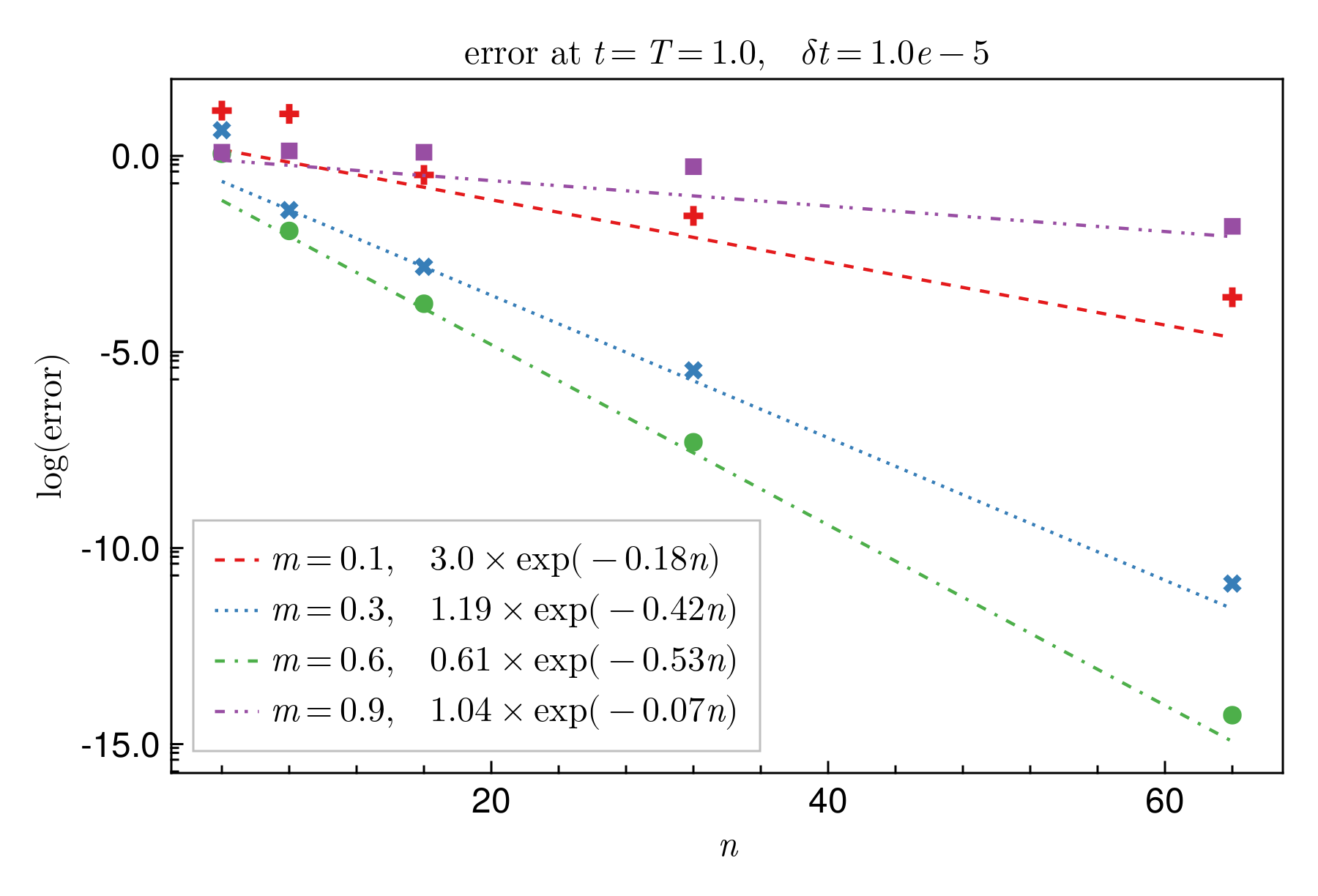
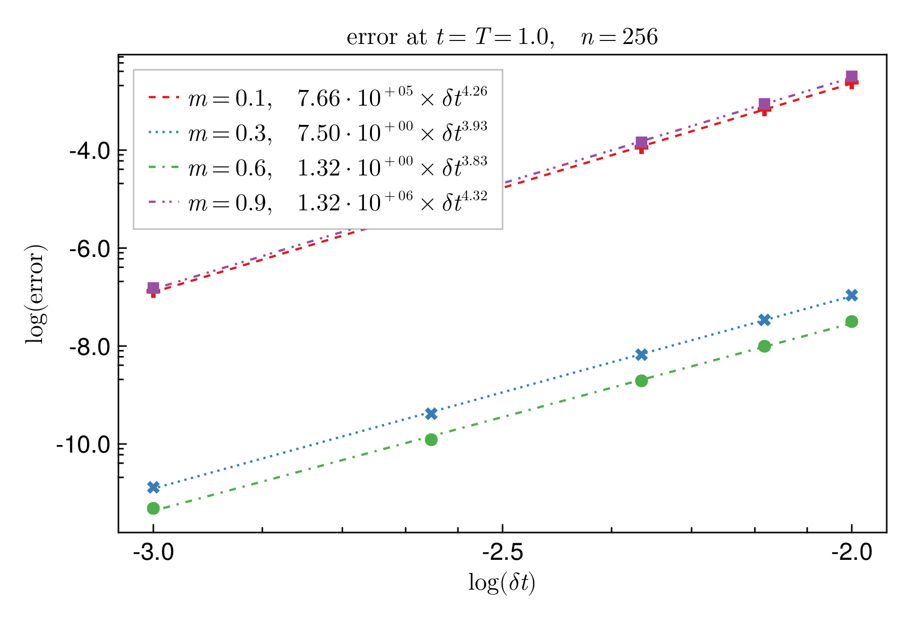
Figure 8. Convergence of the numerical resolution of the reduced dynamical law (24). (Left) Convergence with respect to $n$: as expected, what we observe is compatible with a spectral convergence. (Right) Convergence with respect to $\delta t$: as expected, the convergence is algebraic of order about $4$.

6.2. Numerical convergence of the vortex-tracking method

We focus now on Case 1: there are two vortices with identical winding number $+1$ and initial position $(\pm 0.5,0)$. From Figure 2, we know that we expect, for small values of $\varepsilon$, the vortices to move around the circle of radius $0.5$ and centered at $(0,0)$.

6.2.1. Computational framework

In order to compare the numerical method presented in Section 4 to the exact solution of the GP equation (2), we compute a reference solution $\psi_{\varepsilon}(t)$ with the finite element solver Gridap.jl [3] and meshing tool GMSH [19]. The GP equation (2) is solved for initial conditions given by the vortex configuration from Case 1 and the smoothing procedure described in Lemma 1. We use a Strang splitting scheme, with $\mathbb{P}^{1}$ Lagrangian finite elements for the spatial discretization. The mesh size is of order $h=5\cdot 10^{-2}$ with local a priori refined mesh on the vortex trajectory with mesh size $h=2\cdot 10^{-3}$, see Figure 9. The time step is $\delta t=10^{-5}$. The finite element solver is then used to obtain various reference solutions $\psi_{\varepsilon}$ for $\varepsilon\in\left\{0.03,0.05,0.07,0.1\right\}$, up to $T=1$. We also compute a reference solution for $\varepsilon=0.01$, with time step $\delta t=10^{-6}$.

The reconstructed approximation $\psi_{\varepsilon}^{*}(t)$ from Section 4 is obtained from the trajectories in the limit $\varepsilon\to 0$, with $r_{0}=0.3$ and $n=128$ for the reconstruction step. The Hamiltonian dynamics is solved numerically with a RK4 method, with time step $\delta t=10^{-5}$ and $n=128$.

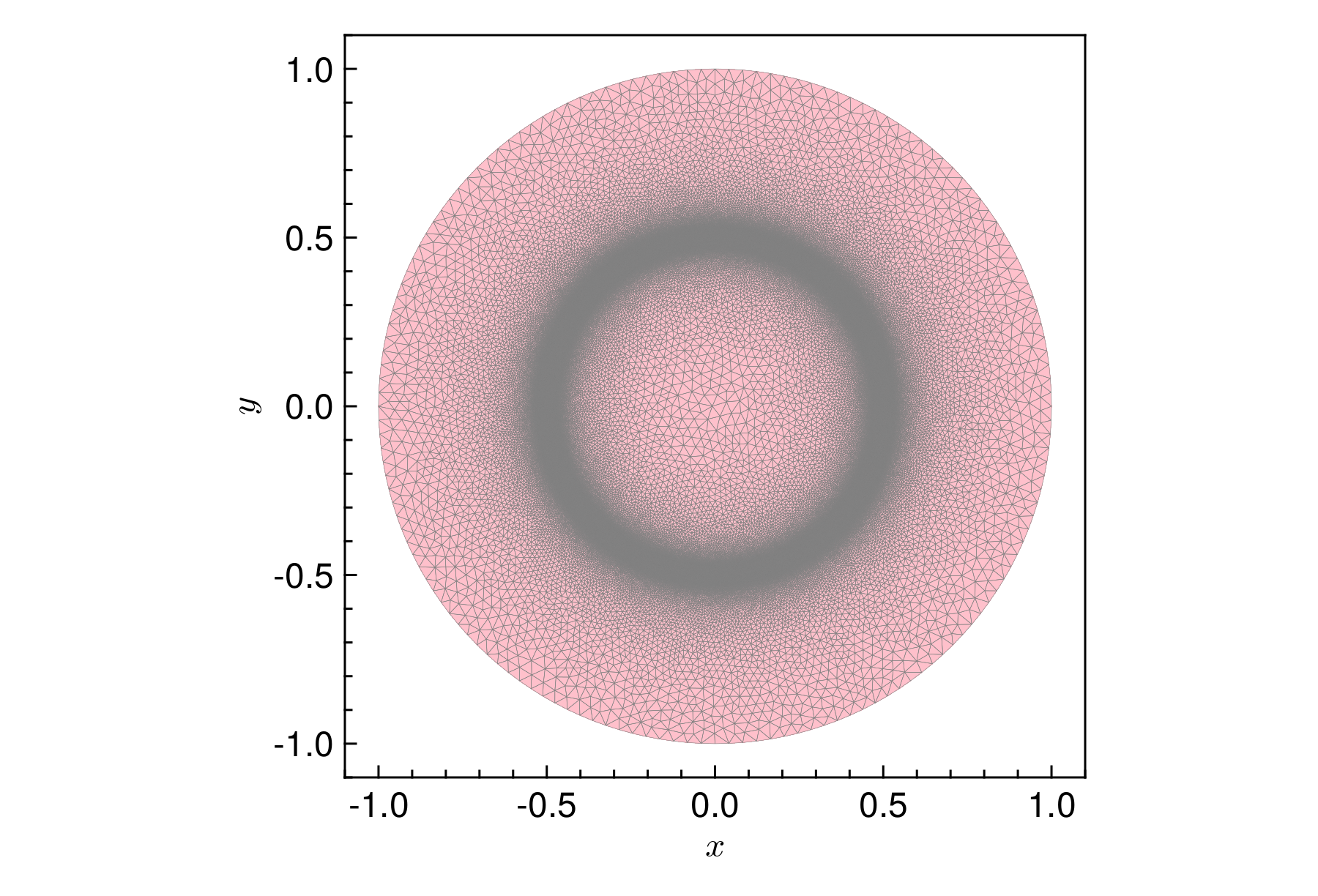
Figure 9. Mesh of the unit disk used to obtain reference solutions.

6.2.2. Numerical illustration of the singular limit $\varepsilon\to 0$

We evaluate different quantities in order to formally compare the reference solution $\psi_{\varepsilon}(t)$ and the reconstructed approximation $\psi_{\varepsilon}^{*}(t)$. First, by tracking its isolated zeros, for instance using one of the algorithms introduced in [14, 26], we are able to localize the vortices of the reference solution $\psi_{\varepsilon}(t)$ and plot the associated trajectories in Figure 10, in the spirit of the study realized in [7]. We observe similar results and, in particular, the oscillations of the vortex trajectories for $\varepsilon>0$ around the limiting trajectory. In Figure 11, we represent the distance between vortices $\left\|{\bm{a}}(t)-P_{h}(\psi_{\varepsilon}(t))\right\|$ as $t$ goes from 0 to $T$, where $P_{h}$ is the vortex localization operator on the finite element mesh. As expected, this error becomes small when $\varepsilon\to 0$. Then, we analyze the (relative) errors on the supercurrents and the wave function (in $L^{2}$ and $H^{1}$ norms), i.e.

$$\frac{\left\|j(\psi_{\varepsilon}(t))-j(\psi_{\varepsilon}^{*}(t))\right\|_{L^{\frac{4}{3}}}}{\left\|j(\psi_{\varepsilon}(t))\right\|_{L^{\frac{4}{3}}}},\quad\frac{\left\|\psi_{\varepsilon}(t)-\psi_{\varepsilon}^{*}(t)\right\|_{L^{2}}}{\left\|\psi_{\varepsilon}(t)\right\|_{L^{2}}}\quad\text{and}\quad\frac{\left\|\nabla\psi_{\varepsilon}(t)-\nabla\psi_{\varepsilon}^{*}(t)\right\|_{L^{2}}}{\left\|\nabla\psi_{\varepsilon}(t)\right\|_{L^{2}}}.$$ (57)

Again, these quantities are smaller for small values of $\varepsilon$, as expected.

Finally, we compare in Figure 12 the relative error in the $L^{2}$ norm when approximating $\psi_{\varepsilon}(t)$ by $\psi_{\varepsilon}^{*}(t)$ or by the canonical harmonic map $u^{*}(\bm{a}(t),\bm{d})$ as well as for the supercurrents. The error achieved by the reconstructed wave function is slightly better than the one achieved by the canonical harmonic map with singularities located at ${\bm{a}}(t)$. Regarding the supercurrents, the reconstruction procedure seems to improve significantly the approximation.

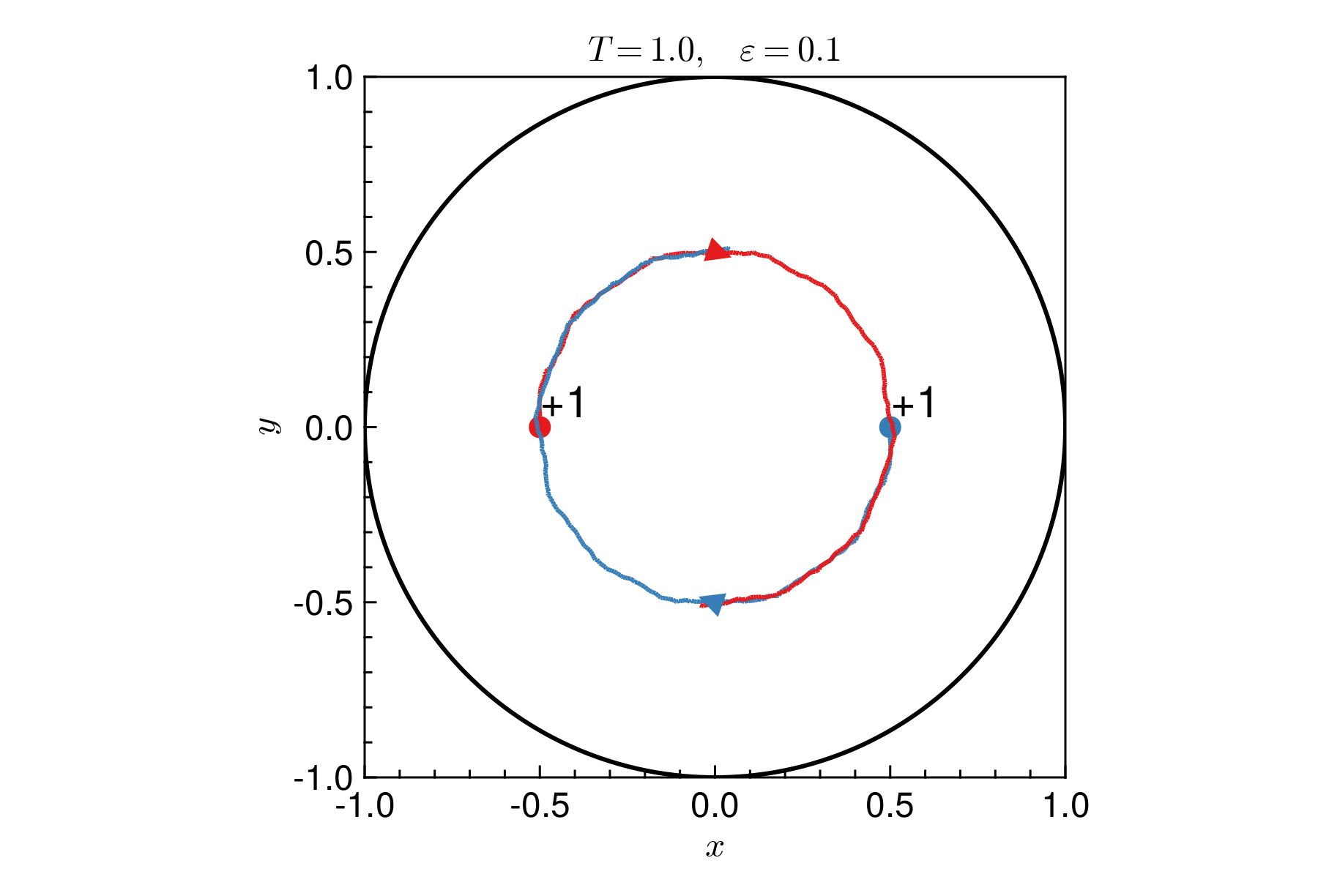
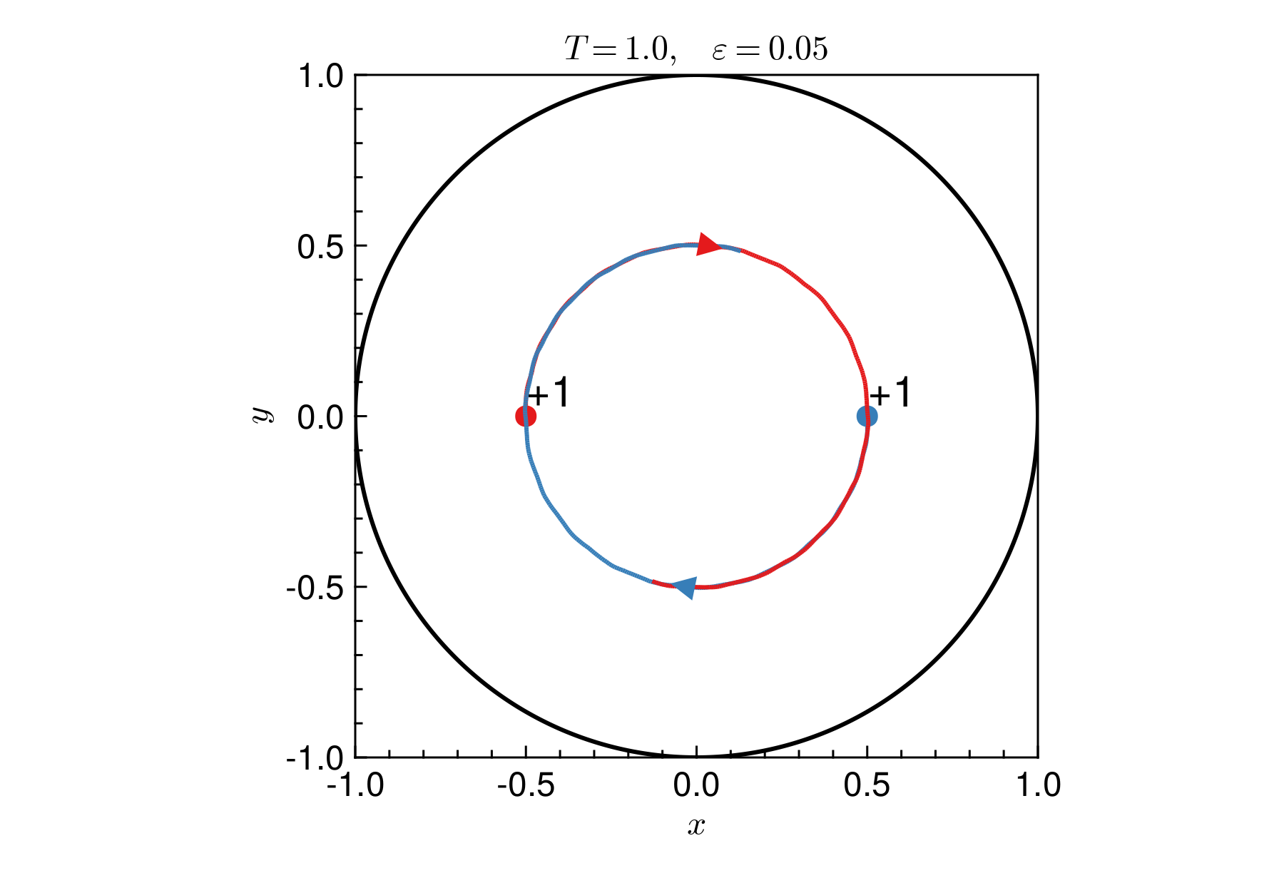
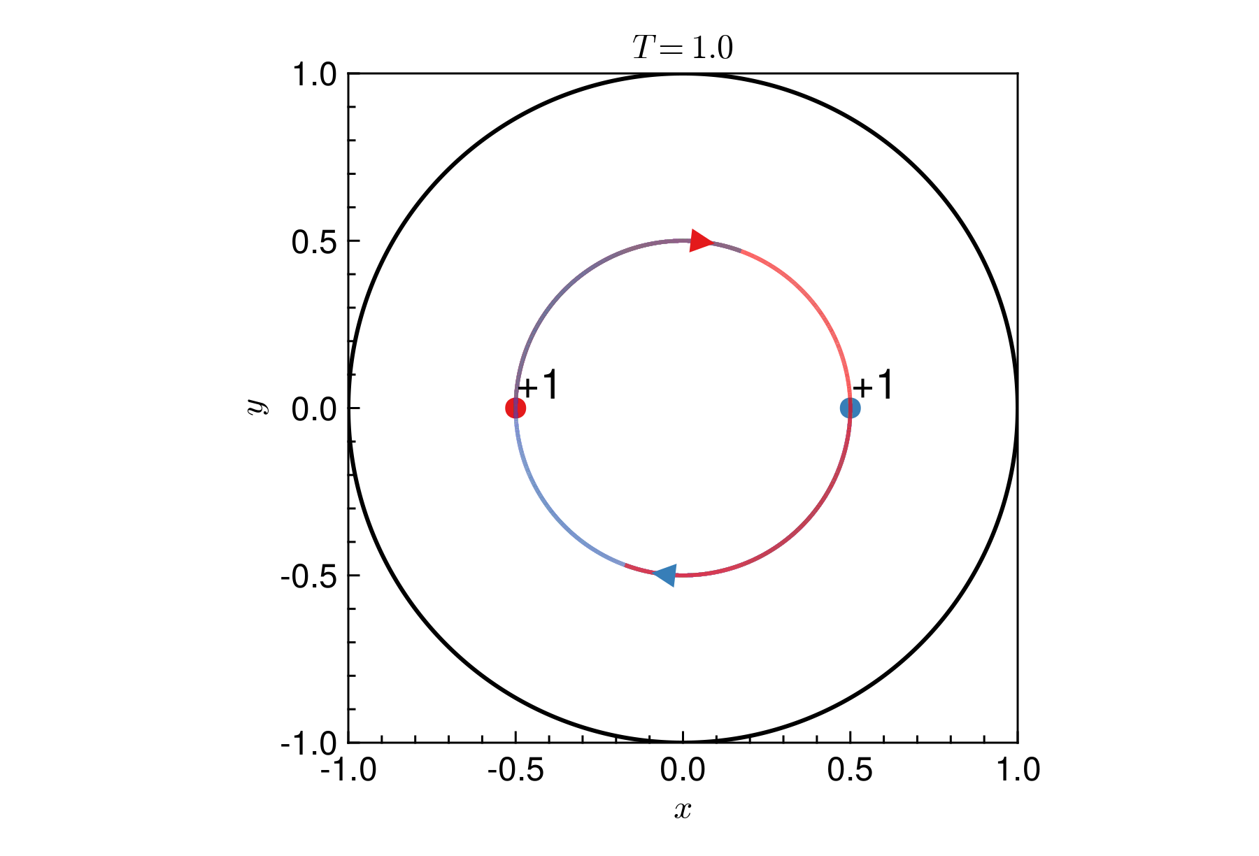
Figure 10. Vortex trajectories in the limit case for different values of $\varepsilon>0$ and for $\varepsilon=0$ (bottom right). For finite $\varepsilon$, the trajectories oscillate around the limit trajectory.

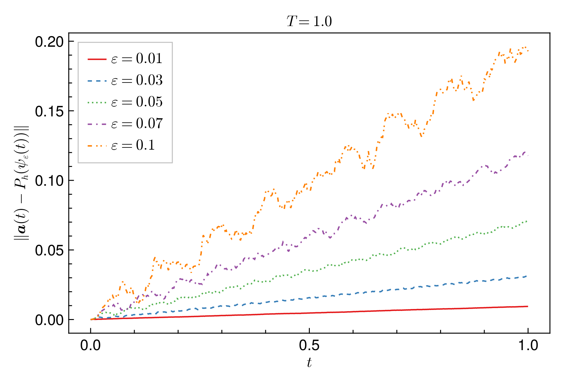
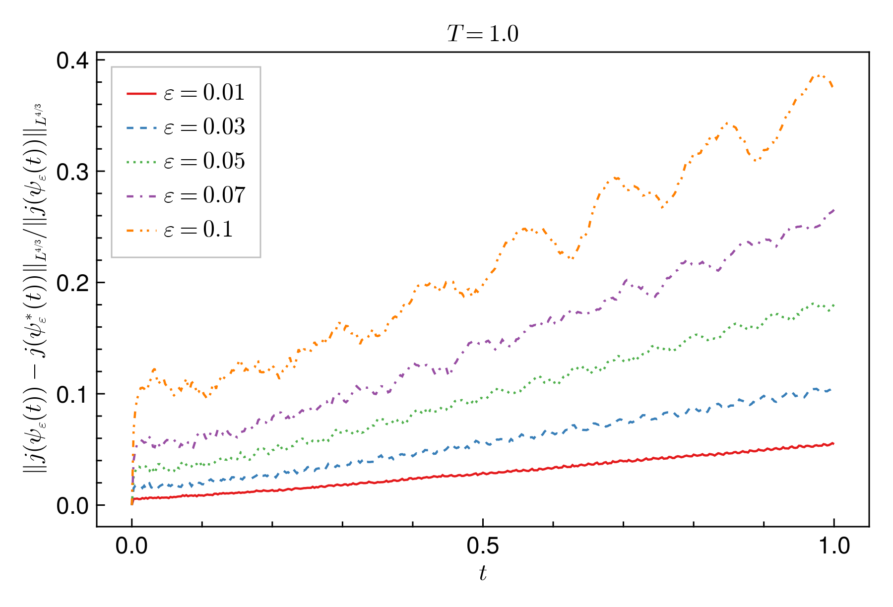
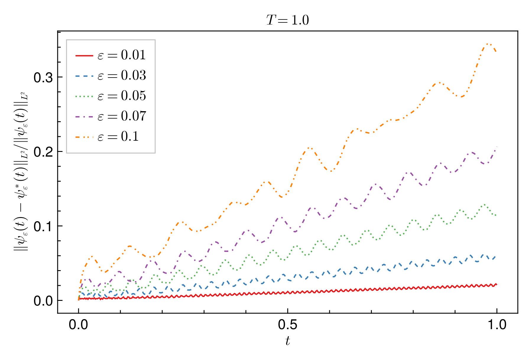
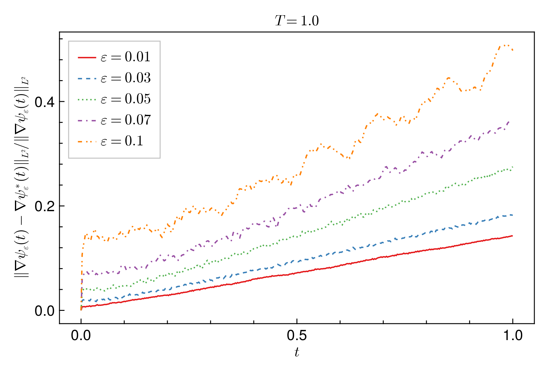
Figure 11. Error on different quantities up to time $T$ for case 1. (Top left) Error on vortices positions in $\Omega$. (Top right) $L^{\frac{4}{3}}$ norm of the error on the supercurrents. (Bottom left) $L^{2}$ norm of the error between $\psi_{\varepsilon}(t)$ and the reconstructed wave function $\psi_{\varepsilon}^{*}(t)$. (Bottom right) $L^{2}$ norm of the error between $\nabla\psi_{\varepsilon}(t)$ and the reconstructed gradient $\nabla\psi_{\varepsilon}^{*}(t)$. .

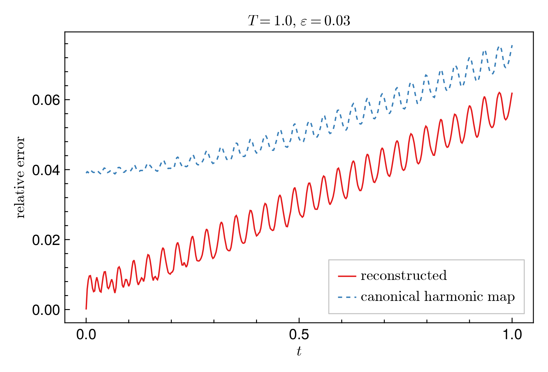
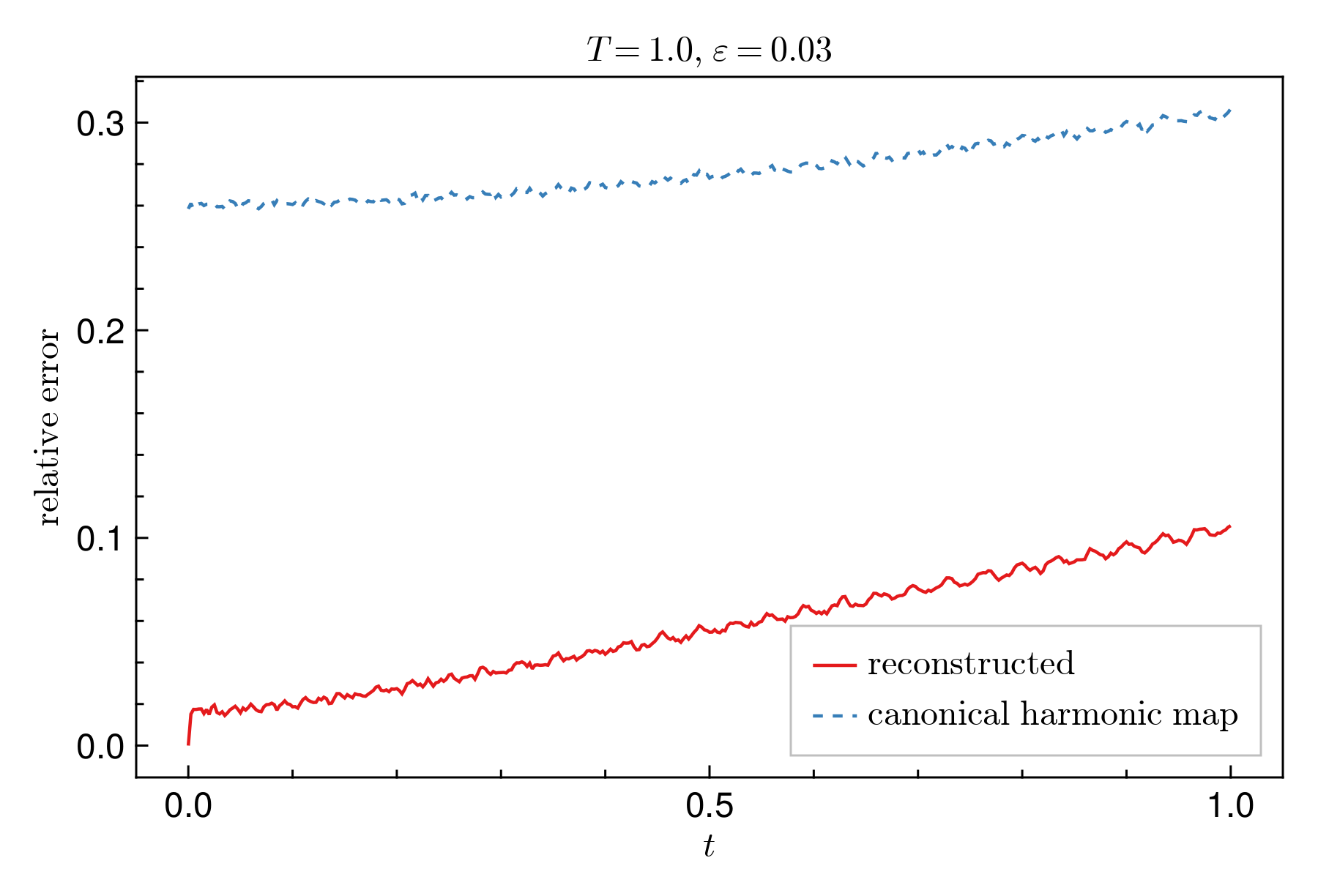
Figure 12. (Left) $L^{2}$ norm of the error between $\psi_{\varepsilon}(t)$ and the canonical harmonic map $u^{*}({\bm{a}}(t),d)$ vs the error between $\psi_{\varepsilon}(t)$ and $\psi_{\varepsilon}^{*}(t)$, for $\varepsilon=0.03$. (Right) $L^{\frac{4}{3}}$ norm of the error between $j(\psi_{\varepsilon}(t))$ and $j(u^{*}({\bm{a}}(t),d))$ vs the error between $j(\psi_{\varepsilon}(t))$ and $j(\psi_{\varepsilon}^{*}(t))$, for $\varepsilon=0.03$.

6.2.3. Numerical illustration of Theorem 2

We end this section by a numerical illustration of Theorem 2 and the convergence with respect to $\varepsilon$. Indeed, with $\delta=10^{-5}$ and $n=128$, the previous numerical considerations lead to a dominating error contribution coming from $\varepsilon>0$. From Theorem 2, we expect it to be of order $\varepsilon^{\gamma}$, with some exponent $\gamma$. In Figure 13, we plot a linear regression in $\varepsilon$ of the error

$$\left\|j(\psi_{\varepsilon}(t))-j(\psi_{\varepsilon}^{*}(t))\right\|_{L^{\frac{4}{3}}}\quad\text{and}\quad\left\|j(\psi_{\varepsilon}(t))-j(u^{*}(\bm{a}(t),d)\right\|_{L^{\frac{4}{3}}},\quad$$

for different times $t$ and $\varepsilon\in\left\{0.01,0.03,0.05,0.07,0.1\right\}$. The linear regression suggests an exponent $\gamma>1/2$ for the first error and $\gamma$ closer to $\frac{1}{2}$ for the second error. The latter is expected from (36), and the first plot therefore suggests that the smoothing procedure reduces the error when approximating $j(\psi_{\varepsilon}(t))$ by $j(\psi_{\varepsilon}^{*}(t))$.

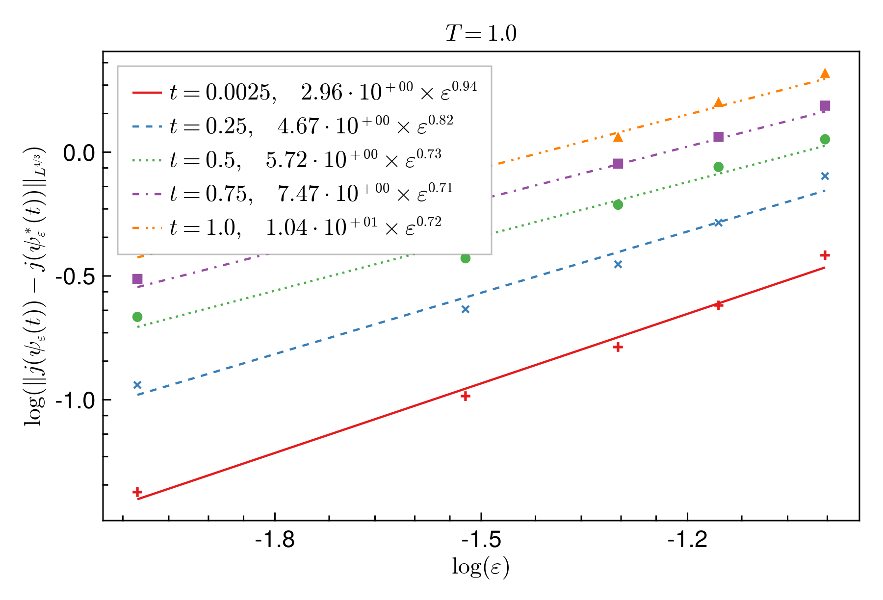
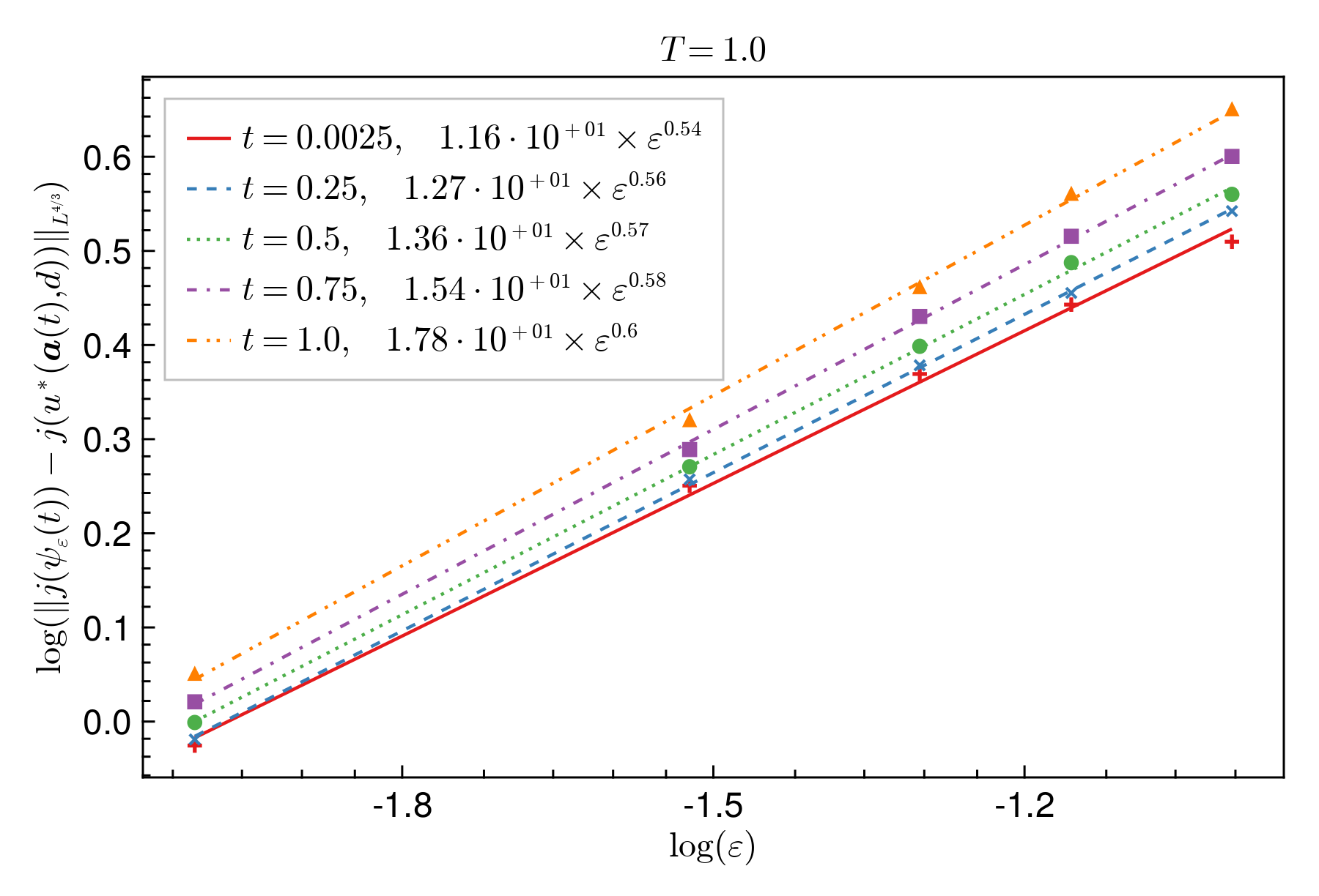
Figure 13. Linear regression in $\varepsilon$ on $\left\|j(\psi_{\varepsilon}(t))-j(\psi_{\varepsilon}^{*}(t))\right\|_{L^{\frac{4}{3}}}$ (left) and $\left\|j(\psi_{\varepsilon}(t))-j(u^{*}({\bm{a}}(t),d)\right\|_{L^{\frac{4}{3}}}$ (right), at different times $t$.

7. Conclusion

In this paper, we introduced a new method for the numerical simulation of the Gross–Pitaevskii equation in the regime of small vortices of core size $\varepsilon\ll 1$. From a computational point of view, this is a very demanding task as small vortices require very fine spatial and time discretization to ensure numerical stability. Based on the analytical theory of the singular limit $\varepsilon\to 0$, we introduced a cheap, efficient and asymptotically valid numerical method. We believe our method to have two main advantages: (i) the numerical treatment of $\varepsilon$ is necessary in a pre-processing step only, where the one-dimensional ODE (30) can be solved accurately, and (ii) the numerical solution is asymptotically valid, in the sense that the smaller $\varepsilon$, the more accurate is the numerical approximation. We also provided error estimates on the supercurrents in the case where $\Omega$ is the unit disk, with numerical illustration of the convergence. We expect this method to work in more general cases where the vortex motion can be reduced to a system of ODE, for instance when using the gradient flow or mixed flow instead of the Schrödinger flow, see e.g. [6, 29, 34], or when adding a magnetic field [21, 34].

Appendix A Error estimates

In this section we derive some error estimates used in the proof of Theorem 2. There are two main sources of error for our numerical scheme: (i) the evaluation of the forcing term of the ODE requires to solve a PDE at each time step which introduces a first discretization error, and (ii) the numerical resolution of the ODE itself introduces a time discretization error.

In all this appendix, we consider, for $s\in\mathbb{R}$, the fractional Sobolev spaces $H^{s}(\partial\Omega)$ equipped with norm

$$\left\|g\right\|_{H^{s}(\partial\Omega)}^{2}=2\pi\sum_{k\in\mathbb{Z}}(1+|k|^{2})^{s}|\widehat{g}(k)|^{2},$$

where the Fourier coefficients are defined by

$$\widehat{g}(k)=\frac{1}{2\pi}\int_{0}^{2\pi}e^{-\imath k\theta}g(e^{\imath\theta})\mathrm{d}\theta.$$

A.1. Exact vs approximate forcing term

According to Section 3, we are interested in the solution $\bm{a}\leavevmode\nobreak\ :\leavevmode\nobreak\ \mathbb{R}_{+}\leavevmode\nobreak\ \rightarrow\leavevmode\nobreak\ \Omega^{*N}$ of the ODE

$$\begin{cases}\dot{\bm{a}}(t)=F\bigr{(}\bm{a}(t)\bigr{)},\quad t\in\mathbb{R}_{+}\\ \bm{a}(0)=\bm{a_{0}}\in\Omega^{*N},\end{cases}$$ (58)

where the components $F_{j}:\Omega^{*N}\rightarrow\mathbb{R}^{2}$ of the forcing term $F(\bm{a})=(F_{1}(\bm{a}),...,F_{N}(\bm{a}))\in\mathbb{R}^{2N}$ are given by

$$F_{j}(\bm{a})=2\mathbb{J}\biggr{(}\nabla_{x}R(x;\bm{a},d)\bigr{\rvert}_{x=a_{j}}+\sum_{k\neq j}^{N}d_{k}\frac{a_{j}-a_{k}}{|a_{j}-a_{k}|}\biggr{)}\quad\quad\mbox{for some }\{d_{j}\}_{j=1}^{N}\in\{\pm 1\}^{N},$$

and $R(\cdot;\bm{a},d):\Omega\rightarrow\mathbb{R}$ is the solution of

$$\begin{cases}\Delta_{x}R(x;\bm{a},d)=0,\quad\text{in }\Omega,\\ \displaystyle R(x;\bm{a},d)=-\sum_{j=1}^{N}d_{j}\log|x-a_{j}|\quad\text{on }\partial\Omega.\end{cases}$$

After fixing the basis of harmonic polynomials up to order $n$, the approximate forcing term we evaluate is

$$F_{j}^{n}(\bm{a})=2\mathbb{J}\biggr{(}\nabla_{x}R_{n}(x;\bm{a},d)\bigr{\rvert}_{x=a_{j}}+\sum_{k\neq j}^{N}d_{k}\frac{a_{j}-a_{k}}{|a_{j}-a_{k}|}\biggr{)}\quad\quad\mbox{for some }\{d_{j}\}_{j=1}^{N}\in\{\pm 1\}^{N},$$

with $R_{n}(\cdot;\bm{a},d):\Omega\rightarrow\mathbb{R}$ being the solution of

$$\begin{cases}\Delta_{x}R_{n}(x;\bm{a},d)=0,\quad\text{in }\Omega,\\ \displaystyle R_{n}(x;\bm{a},d)=-\mathbb{P}_{n}\biggr{(}\sum_{j=1}^{N}d_{j}\log|x-a_{j}|\biggr{)},\quad\text{on }\partial\Omega,\end{cases}$$

where $\mathbb{P}_{n}$ is the $L^{2}(\partial\Omega)$-orthogonal projection on the bases of harmonic polynomials up to order $n$ on the boundary. Our task is to estimate the difference $R_{n}-R$ in suitable norms. To this end, we shall use the following well-known estimates.

Lemma 3 (Classical estimates for Dirichlet problem [20]).

Let $\Omega\subset\mathbb{R}^{2}$ be a bounded smooth domain, $g\leavevmode\nobreak\ \in\leavevmode\nobreak\ C^{\infty}(\partial\Omega)$, and $u\in C^{\infty}(\overline{\Omega})$ be the unique solution of

$$\begin{cases}\Delta u=0,\quad\mbox{in $\Omega$,}\\ u=g,\quad\mbox{in $\partial\Omega$.}\end{cases}$$ (59)

Then there exists implicit constants depending only on $\Omega$ and $\ell\in\mathbb{N}\cup\{0\}$ such that

$$|\partial^{\alpha}u(x)|\lesssim_{\ell}\frac{1}{\operatorname{dist}(x,\partial\Omega)^{\frac{1}{2}+\ell}}\left\|g\right\|_{L^{2}(\partial\Omega)}\quad\mbox{for any $\alpha\in(\mathbb{N}\cup\{0\})^{2}$ with $|\alpha|=\ell$,}$$ (60)

$$\left\|\nabla u\right\|_{L^{2}(\Omega)}\lesssim\left\|g\right\|_{H^{\frac{1}{2}}(\partial\Omega)}.$$ (61)

Moreover, in the case where $\Omega$ is the unit disk and $\mathbb{P}_{n}g=0$, there exists constants independent of $n$, $g$, and $x\in\Omega$ such that

$$|\partial^{\alpha}u(x)|\lesssim_{\ell}\frac{n^{\ell}|x|^{n+1-\ell}}{(1-|x|)^{\frac{1}{2}+\ell}}\left\|g\right\|_{L^{2}(\partial\Omega)},\quad\mbox{for any $\alpha\in(\mathbb{N}\cup\{0\})^{2}$ with $|\alpha|=\ell\geq 1$.}$$ (62)

$$\left\|\nabla u\right\|_{L^{2}(\Omega)}^{2}=\sum_{|k|>n}2\pi|k||\widehat{g}(k)|^{2}.$$ (63)

Proof.

Estimate (60) and (61) are rather classical and detailed proofs can be found in [20, Section 2.7]. Let us thus focus on the specific estimate for the disk and briefly sketch the argument in the general case. First, note that for the disk, we have the explicit formula for the solution via the Poisson kernel $P_{r}(\theta)$ or, equivalently, via the Fourier coefficients of $g$,

$$u(re^{\imath\theta})=-\frac{1}{2\pi}\int_{0}^{2\pi}P_{r}(\theta-\phi)g(e^{\imath\phi})\mathrm{d}\phi=\sum_{k\in\mathbb{Z}}r^{|k|}\widehat{g}(k)e^{\imath k\theta}.$$

Now, note that the harmonic polynomials of order up to $n$ span the same space as $\{z^{k}\}_{k=0}^{n}\cup\{\overline{z}^{k}\}_{k=1}^{n}$, which are just the Fourier basis if restricted to the boundary. In particular, if $\mathbb{P}_{n}g=0$, then the above sum runs over the integers $|k|>n$. From the orthogonality of $r^{|k|}e^{\imath k\theta}$ on $L^{2}(\Omega)$, we then have

$$\left\|u\right\|_{L^{2}(\Omega)}^{2} =\sum_{|k|>n}|\widehat{g}(k)|^{2}\left\||r|^{k}e^{\imath k\theta}\right\|_{L^{2}(\Omega)}^{2}=\sum_{|k|>n}\frac{\pi}{|k|+1}|\widehat{g}(k)|^{2}.$$

Moreover, we can express the radial and angular component of the (a priori weak) gradient of $u$ as

$$\partial_{r}u(re^{\imath\theta})=\sum_{|k|>n}|k|\widehat{g}(k)r^{|k|-1}e^{\imath k\theta}\quad\mbox{and}\quad\frac{1}{r}\partial_{\theta}u(re^{\imath\theta})=\sum_{|k|>n}\imath k\widehat{g}(k)r^{|k|-1}e^{\imath k\theta}.$$

Consequently, from Cauchy-Schwarz we find

$$|\nabla u(re^{\imath\theta})|^{2} \leq 2\biggr{(}\sum_{|k|>n}|\widehat{g}(k)|^{2}\biggr{)}\biggr{(}2\sum_{k>n}k^{2}r^{2(k-1)}\biggr{)}$$

$$=\frac{1}{\pi}\left\|g\right\|_{L^{2}(\partial\Omega)}^{2}\biggr{(}\frac{2r^{2n}}{(1-r^{2})^{3}}\underbrace{\bigr{(}n^{2}r^{4}-(2n^{2}+2n-1)r^{2}+(n+1)^{2}\bigr{)}}_{\leq(n+1)^{2}\text{ for }r\in[0,1]}\biggr{)}$$

$$\leq\frac{2}{\pi}\frac{(n+1)^{2}r^{2n}}{(1-r)^{3}}\left\|g\right\|_{L^{2}(\partial\Omega)}^{2},$$ (64)

$$\left\|\nabla u\right\|_{L^{2}(\Omega)}^{2} =\int_{0}^{1}\int_{0}^{2\pi}\biggr{(}|\partial_{r}u|^{2}+\frac{1}{r^{2}}|\partial_{\theta}u|^{2}\biggr{)}r\mathrm{d}r\mathrm{d}\theta$$

$$=\sum_{|j|,|k|>n}\overline{\widehat{g}(k)}\widehat{g}(j)\biggr{(}|k||j|\langle r^{|k|-1}e^{\imath k\theta},r^{|j|-1}e^{\imath j\theta}\rangle_{L^{2}(\Omega)}+kj\langle r^{|k|-1}e^{\imath k\theta},r^{|j|-1}e^{\imath j\theta}\rangle_{L^{2}(\Omega)}\biggr{)}$$

$$=\sum_{|k|>n}2\pi|k||\widehat{g}(k)|^{2}\leq\left\|g\right\|_{H^{\frac{1}{2}}(\partial\Omega)}^{2},$$ (65)

which completes the proof of the first part for $\ell=1$. The general $\ell$ case follows from the same steps by noticing that each radial and angular derivative gives a factor of $k/r$ in the series, and using the bound

$$\sum_{k>n}k^{2\ell}r^{2k}\lesssim_{\ell}\frac{n^{2\ell}r^{2n+2}}{(1-r)^{2\ell+1}},\quad\ell\in\mathbb{N},$$

which follows by induction on (or differentiating) the well-known formula for the partial sums of the geometric series.

For the general smooth domain case, one can apply a biholomorphic conformal transformation of $\Omega$ into the disk. As the transformation and its inverse are smooth up to the boundary (see, e.g. [28, Chapter 5]) the $L^{2}$ and $H^{\frac{1}{2}}$ norm on the boundary of $\Omega$ are, respectively, equivalent to the $L^{2}$ and $H^{\frac{1}{2}}$ norms on the circle. Therefore, eqs. (60) and (61) follows from (64) and (65). ∎

Lemma 4 (Log function estimates).

Let $(a,b)\in\Omega^{*2}$ and $g_{a}(x)=\log|x-a|$, then we have

$$\left\|g_{a}-g_{b}\right\|_{H^{s}(\partial\Omega)}\lesssim_{s}\frac{|a-b|}{\min\{\operatorname{dist}(a,\partial\Omega)\operatorname{dist}(b,\partial\Omega)\}^{s+1}}\quad\mbox{for any $0\leq s\leq 1$,}$$ (66)

$$\left\|\nabla g_{a}-\nabla g_{b}\right\|_{L^{p}(\Omega)}\lesssim|a-b|^{\frac{2}{p}-1},\quad\mbox{for any $1\leq p<2$}$$ (67)

$$\left\|g_{a}\right\|_{H^{\ell}(\partial\Omega)}\lesssim\frac{1}{\operatorname{dist}(a,\partial\Omega)^{\max\{\ell-\frac{1}{2},0\}}},\quad\mbox{for any $\ell\in\mathbb{N}\cup\{0\}.$}$$ (68)

Moreover, if $\Omega$ is the unit disk we have

$$\left\|\mathbb{P}_{n}^{\perp}g_{a}\right\|_{H^{s}(\partial\Omega)}\lesssim_{\ell}\frac{n^{-\ell+s}}{\operatorname{dist}(a,\partial\Omega)^{\ell-\frac{1}{2}}}\quad\mbox{for any $0\leq s\leq\ell$ and $\ell\geq 1$,}$$ (69)

where $\mathbb{P}_{n}^{\perp}=1-\mathbb{P}_{n}$ and $\mathbb{P}_{n}$ is the orthogonal projection defined previously and the implicit constants are independent of $a,b$ and $n$.

Proof.

Since $\nabla\log|x|=x/|x|^{2}$ is positively homogeneous of degree $-1$, we find $\big{|}\nabla^{k}\log|x|\big{|}\lesssim_{k}|x|^{-k}$ for any $k\in\mathbb{N}$. In fact, by induction one can show that for any $\alpha\in\mathbb{N}^{2}$ with $|\alpha|\geq 1$ we have

$$\partial^{\alpha}\log|x|=\frac{p_{\alpha}(x)}{|x|^{2|\alpha|}},\quad\mbox{for some polynomial $p_{\alpha}$ homogeneous of degree $|\alpha|$,}$$ (70)

which implies

$$\big{|}\log|x|-\log|y|\big{|}\lesssim\frac{|x-y|}{\min\{|x|,|y|\}}\quad\mbox{and}\quad\big{|}\nabla\log|x|-\nabla\log|y|\big{|}\lesssim\frac{|x-y|}{\min\{|x|,|y|\}^{2}}.$$ (71)

Integrating these estimate along the boundary, we obtain (66) for $s=0$ and $s=1$. The estimates for $0<s<1$ then follow by interpolation.

For the $L^{p}$ estimate in the interior, we split the integration over the balls $B_{\rho}(b)$, $B_{\rho}(a)$, and the rest of the domain $\Omega_{a,b}=\Omega\setminus\bigr{(}B_{\rho}(b)\cup B_{\rho}(a)\bigr{)}$ for some $\rho<|a-b|/2$. Then since the terms $\nabla g_{a}\sim|x-a|^{-1}$ gives the dominant contribution inside the ball $B_{\rho}(a)$, we can use estimate (71) on $\Omega_{a,b}$ to obtain

$$\left\|\nabla g_{a}-\nabla g_{b}\right\|_{L^{p}(\Omega)}^{p} \lesssim\int_{B_{\rho}(b)}\frac{1}{|x-b|^{p}}\mathrm{d}x+\int_{B_{\rho}(a)}\frac{1}{|x-a|^{p}}\mathrm{d}x+\int_{\Omega_{a,b}}\frac{|a-b|^{p}}{\min\{|x-b|,|x-a|\}^{2p}}\mathrm{d}x$$

$$\lesssim\rho^{2-p}+\frac{|a-b|^{p}}{\rho^{2p-2}}.$$

Minimizing the right hand-side, we find $\rho\sim|a-b|$, which yields (67).

Lastly, to prove the spectral convergence for the $L^{2}(\partial\Omega)$ norm, we can use (70) again. Indeed, by integrating the function $|x-a|^{-2\ell}$ along the boundary we have

$$\left\|g_{a}\right\|_{H^{\ell}(\partial\Omega)}^{2}\cong\left\|\nabla^{\ell}\log|x-a|\right\|_{L^{2}(\partial\Omega)}^{2}\lesssim\begin{dcases}\operatorname{dist}(a,\partial\Omega)^{-2\ell+1},\quad\mbox{for $\ell\in\mathbb{N}$,}\\ 1,\quad\mbox{for $\ell=0$,}\end{dcases}$$

which proves (68). Since we have the equivalence of norms $\left\|g\right\|_{H^{s}(\partial\Omega)}^{2}\cong\sum_{k\in\mathbb{Z}}|\widehat{g}(k)|^{2}(1+|k|)^{2s}$ on the disk, we find

$$\left\|\mathbb{P}_{n}^{\perp}g_{a}\right\|_{H^{s}(\partial\Omega)}^{2}\cong\sum_{|k|>n}|\widehat{g_{a}}(k)|^{2}(1+|k|)^{2s}\lesssim n^{-2\ell+2s}\left\|g_{a}\right\|_{H^{\ell}(\partial\Omega)}^{2}=\frac{n^{-2\ell+2s}}{\operatorname{dist}(a,\partial\Omega)^{2\ell-1}},\quad\mbox{for $\ell\in\mathbb{N}$.}$$

The case $\ell\geq 1$ for real $\ell$ follows by interpolation. ∎

Let us now denote by $\bm{b}:\mathbb{R}_{+}\to\Omega^{*N}$ the solution of the approximated ODE

$$\begin{cases}\dot{\bm{b}}(t)=F^{n}(\bm{b}(t)),\\ \bm{b}(0)=\bm{b}^{0},\end{cases}$$ (72)

where $F^{n}$ is the approximated forcing term. Then an application of Gronwal’s inequality with the previous estimates yields

Lemma 5 (Continuous dynamical error).

Let $\bm{b}^{0},\bm{a}^{0}\in\Omega^{*N}$ and $\bm{a}(t)$ and $\bm{b}(t)$ be respectively the solutions of (58) and (72), for a fixed $d\in\left\{\pm 1\right\}^{N}$ and let

$$\rho(\bm{a})\coloneqq\min_{j\neq\ell}\{\operatorname{dist}(a_{j},\partial\Omega),|a_{j}-a_{\ell}|\}.$$

Suppose that $\rho_{T}\coloneqq\inf_{t\in[0,T]}\rho\bigr{(}\bm{a}(t)\bigr{)}>0$. Then, there exists some $C=C(\Omega,N)>0$ such that

$$|\bm{a}(t)-\bm{b}(t)|\lesssim\biggr{(}|\bm{a}^{0}-\bm{b}^{0}|+\frac{\sup_{s\in[0,T]}\left\|\mathbb{P}_{n}^{\perp}g_{\bm{a}(s)}\right\|_{L^{2}(\partial\Omega)}}{\rho_{T}^{3/2}}T\biggr{)}e^{Ct/\rho_{T}^{5/2}},\quad\mbox{for any $t\in[0,T]$,}$$ (73)

where $g_{\bm{a}}(x)=-\sum_{j=1}^{N}d_{j}\log|x-a_{j}|$. Moreover, if $\Omega$ is the unit disk we have

$$|\bm{a}(t)-\bm{b}(t)|\lesssim_{\ell}\biggr{(}|\bm{a}^{0}-\bm{b}^{0}|+\frac{(1-\rho_{T})^{n}n^{1-\ell}}{\rho_{T}^{1+\ell}}T\biggr{)}e^{Ct/\rho_{T}^{5/2}},\quad\mbox{for any $t\in[0,T]$,}$$ (74)

and any $\ell\in\mathbb{N}$, where all the implicit constants are independent of $\bm{a}^{0},\bm{b}^{0},n,\rho_{T}$, and $t$.

Proof.

First, we split the error via the triangle inequality as

$$|F^{n}(\bm{b})-F(\bm{a})|\leq\underbrace{\sum_{j=1}^{N}|\nabla_{x}R_{n}(b_{j};\bm{b},d)-\nabla_{x}R_{n}(a_{j};\bm{a},d)|}_{\coloneqq E_{1}(\bm{a},\bm{b})}+\underbrace{\sum_{j=1}^{N}|\nabla R_{n}(a_{j};\bm{a},d)-\nabla R(a_{j};\bm{a},d)|}_{\coloneqq E_{2}(\bm{a})}\\ +\underbrace{\sum_{k\neq j}^{N}\biggr{|}\frac{b_{j}-b_{k}}{|b_{j}-b_{k}|^{2}}-\frac{a_{j}-a_{k}}{|a_{j}-a_{k}|^{2}}\biggr{|}}_{\coloneqq E_{3}(\bm{a},\bm{b})}.$$

From estimate (71), we can bound the third term as

$$E_{3}(\bm{a},\bm{b})\lesssim\frac{|\bm{a}-\bm{b}|}{\min\{\rho(\bm{a}),\rho(\bm{b})\}^{2}}.$$ (75)

For the second error, we note that $R_{n}(\cdot;\bm{a},d)-R(\cdot;\bm{a},d)$ is the solution to Laplace’s equation with boundary data $\mathbb{P}_{n}^{\perp}g_{\bm{a}}$, where $g_{\bm{a}}(x)=-\sum_{j=1}^{N}d_{j}\log(x-a_{j})$. Hence, from estimate (60) with $\ell=1$, we obtain

$$E_{2}(\bm{a})\lesssim\frac{1}{\min_{j}\{\operatorname{dist}(a_{j},\partial\Omega)\}^{\frac{3}{2}}}\left\|\mathbb{P}_{n}^{\perp}g_{\bm{a}}\right\|_{L^{2}(\partial\Omega)}.$$ (76)

To control the last term, we observe (i) that $R_{n}(\cdot;\bm{b},d)-R_{n}(\cdot;\bm{a},d)$ solves Laplace’s equation with boundary data $\mathbb{P}_{n}(g_{\bm{a}}-g_{\bm{b}})$, and (ii) that estimate (60) for the second derivative of $R_{n}(\cdot;\bm{a},d)$ gives an upper bound on the Lipschitz constant of the first derivative. Thus, from estimates (66) and (60), we obtain

$$E_{1}(\bm{a},\bm{b}) \leq\sum_{j=1}^{N}\left|\nabla_{x}R_{n}(a_{j};\bm{a},d)-\nabla_{x}R_{n}(a_{j};\bm{b},d)\right|+\left|\nabla_{x}R_{n}(a_{j};\bm{b},d)-\nabla_{x}R_{n}(b_{j};\bm{b},d)\right|$$

$$\lesssim\frac{\left\|\mathbb{P}_{n}(g_{\bm{a}}-g_{\bm{b}})\right\|_{L^{2}(\partial\Omega)}}{\min_{j}\{\operatorname{dist}(a_{j},\partial\Omega)\}^{\frac{3}{2}}}+\frac{|\bm{a}-\bm{b}|}{\min_{j}\{\operatorname{dist}(b_{j},\partial\Omega)\}^{\frac{5}{2}}}\left\|\mathbb{P}_{n}g_{\bm{b}}\right\|_{L^{2}(\partial\Omega)}$$

$$\lesssim|\bm{a}-\bm{b}|\frac{1}{\min_{j}\{\operatorname{dist}(b_{j},\partial\Omega),\operatorname{dist}(a_{j},\partial\Omega)\}^{\frac{5}{2}}},$$ (77)

where we used that $\left\|g_{\bm{a}}\right\|_{L^{2}(\partial\Omega)}\lesssim 1$ with a constant independent of $\bm{a}$ because the logarithm function is locally integrable on $\mathbb{R}$. Summing up estimates (75), (76), and (77), using the assumption $\rho_{T}>0$, and the definition of $\bm{a}(t)$ and $\bm{b}(t)$ we find

$$|\dot{\bm{a}}(t)-\dot{\bm{b}}(t)|\lesssim\frac{|\bm{a}(t)-\bm{b}(t)|}{\rho_{T}^{\frac{5}{2}}}+\frac{\left\|\mathbb{P}_{n}^{\perp}g_{\bm{a}(t)}\right\|_{L^{2}(\partial\Omega)}}{\rho_{T}^{\frac{3}{2}}},$$

from which we obtain (73) after applying Gronwal’s inequality. For the estimate in the disk, one can simply apply (62) and (69) instead of (60) to estimate the $E_{2}(\bm{a})$ term.

∎

A.2. Time discretization

The time integration error follows easily from the previous bounds and standard considerations on the numerical integration of ODE, that we briefly recall here.

Lemma 6.

Let $\bm{b}$ be the exact solution to $\dot{\bm{b}}=F^{n}(\bm{b})$ and let $(\bm{b}_{\delta t}^{k})_{k\delta t\leq T}$ be its numerical approximation with a RK4 method and time step $\delta t$:

$$\begin{cases}\dot{\bm{b}}=F^{n}(\bm{b}),\\ \bm{b}(0)=\bm{b}^{0},\end{cases}\quad\begin{cases}\bm{b}_{\delta t}^{k}=\bm{b}_{\delta t}^{k-1}+\delta t\Phi_{\delta t,n}(\bm{b}_{\delta t}^{k-1}),\\ \bm{b}_{\delta t}^{0}=\bm{b}^{0},\end{cases}$$

where $\Phi_{\delta t,n}$ is the RK4 increment function associated with the approximate forcing term $F^{n}$ (see for instance [22, Chapter II]). Assume that

$$0<\rho_{T}=\min\left(\inf_{0\leq t\leq T}\rho(\bm{b}(t)),\min_{k\delta t\leq T}\rho(\bm{b}^{k}_{\delta t})\right).$$

Then, there exists constants $C_{\rho_{T}}>0$ and $\Lambda_{\rho_{T}}$, that depends on $\rho_{T}$ but not on $n$, $\bm{b}$ or $\delta t$, such that the following global in time error bound holds:

$$\max_{k\delta t\leq T}|\bm{b}(k\delta t)-\bm{b}_{\delta t}^{k}|\leq\delta t^{4}\frac{C_{\rho_{T}}}{\Lambda_{\rho_{T}}}\left(e^{\Lambda_{\rho_{T}}T}-1\right).$$

Proof.

First, we recall, using notations from the proof of Lemma 5, that

$$\forall\ \bm{a},\bm{b}\in\Omega,\quad|F^{n}(\bm{a})-F^{n}(\bm{b})|\leq E_{1}(\bm{a},\bm{b})+E_{3}(\bm{a},\bm{b})\lesssim\frac{|\bm{a}-\bm{b}|}{\min_{j}\left\{\operatorname{dist}(a_{j},\partial\Omega),\operatorname{dist}(b_{j},\partial\Omega)\right\}^{5/{\color[rgb]{1,0,0}2}}}+\frac{|\bm{a}-\bm{b}|}{\min(\rho(\bm{a}),\rho(\bm{b}))^{{\color[rgb]{1,0,0}2}}},$$

with constants that do not depend on $n$. Thus, since

$$0<\rho_{T}=\min\left(\inf_{0\leq t\leq T}\rho(\bm{b}(t)),\min_{k\delta t\leq T}\rho(\bm{b}^{k}_{\delta t})\right),$$

the function $F^{n}$ is Lipschitz continuous on the domain of interest with a Lipschitz constant $\Lambda_{\rho_{T}}$ independent of $n$. To conclude, note that $|\nabla_{\bm{b}}^{4}F^{n}(\bm{b})|\leq C$ for some $C>0$ independent of $n$ and $\bm{b}$, as long as $\rho_{T}>0$ (this follows from the linearity of Laplace’s equation and estimates (60) and (68)). As a result, the local truncation error can be bounded as follows: there exists $C_{\rho_{T}}>0$, independent of $n$, such that

$$|\bm{b}(\delta t)-\bm{b}^{1}_{\delta t}|\leq C_{\rho_{T}}{\delta t}^{5}.$$

Thus, by combining the local truncation error and the Lipschitz continuity of the numerical integrator, we obtain the global in time error bound (see [22, Theorem II.3.6]). ∎

References

- [1] A. Aftalion and P. Mason. Rotation of a Bose-Einstein condensate held under a toroidal trap. Physical Review A, 81(2):023607, 2010.
- [2] X. Antoine, W. Bao, and C. Besse. Computational methods for the dynamics of the nonlinear Schrödinger/Gross–Pitaevskii equations. Computer Physics Communications, 184(12):2621–2633, 2013.
- [3] S. Badia and F. Verdugo. Gridap: An extensible Finite Element toolbox in Julia. Journal of Open Source Software, 5(52):2520, 2020.
- [4] W. Bao, Q. Du, and Y. Zhang. Dynamics of Rotating Bose–Einstein Condensates and its Efficient and Accurate Numerical Computation. SIAM Journal on Applied Mathematics, 66(3):758–786, 2006.
- [5] W. Bao and D. Jaksch. An Explicit Unconditionally Stable Numerical Method for Solving Damped Nonlinear Schrödinger Equations with a Focusing Nonlinearity. SIAM Journal on Numerical Analysis, 41(4):1406–1426, 2003.
- [6] W. Bao and Q. Tang. Numerical Study of Quantized Vortex Interaction in the Ginzburg-Landau Equation on Bounded Domains. Communications in Computational Physics, 14(3):819–850, 2013.
- [7] W. Bao and Q. Tang. Numerical Study of Quantized Vortex Interactions in the Nonlinear Schrödinger Equation on Bounded Domains. Multiscale Modeling & Simulation, 12(2):411–439, 2014.
- [8] T. Bartsch. Periodic solutions of singular first-order Hamiltonian systems of N-vortex type. Archiv der Mathematik, 107(4):413–422, 2016.
- [9] F. Bethuel, H. Brezis, and F. Hélein. Ginzburg-Landau Vortices. Birkhäuser Boston, Boston, MA, 1994.
- [10] M. Brachet. Gross–Pitaevskii description of superfluid dynamics at finite temperature: A short review of recent results. Comptes Rendus Physique, 13(9-10):954–965, 2012.
- [11] H. Brezis, J.-M. Coron, and E. H. Lieb. Harmonic maps with defects. Communications in Mathematical Physics, 107(4):649–705, 1986.
- [12] J. Colliander and R. Jerrard. Vortex dynamics for the Ginzburg-Landau-Schrodinger equation. International Mathematics Research Notices, 1998(7):333, 1998.
- [13] B. Dörich and P. Henning. Error bounds for discrete minimizers of the Ginzburg–Landau energy in the high-\kappa regime, 2023.
- [14] G. Dujardin, I. Lacroix-Violet, and A. Nahas. A numerical study of vortex nucleation in 2D rotating Bose-Einstein condensates. 2022.
- [15] W. E. Dynamics of vortices in Ginzburg-Landau theories with applications to superconductivity. Physica D: Nonlinear Phenomena, 77(4):383–404, 1994.
- [16] A. L. Fetter, P. C. Hohenberg, and P. Pincus. Stability of a Lattice of Superfluid Vortices. Physical Review, 147(1):140–152, 1966.
- [17] C. Gallo. Schrödinger group on Zhidkov spaces. Advances in Differential Equations, 9(5-6), 2004.
- [18] P. Gérard. The Cauchy problem for the Gross–Pitaevskii equation. Annales de l’Institut Henri Poincaré C, Analyse non linéaire, 23(5):765–779, 2006.
- [19] C. Geuzaine and J.-F. Remacle. Gmsh: A 3-D finite element mesh generator with built-in pre- and post-processing facilities: THE GMSH PAPER. International Journal for Numerical Methods in Engineering, 79(11):1309–1331, 2009.
- [20] D. Gilbarg and N. S. Trudinger. Elliptic Partial Differential Equations of Second Order, volume 224 of Classics in Mathematics. Springer Berlin Heidelberg, Berlin, Heidelberg, 2001.
- [21] S. Gustafson and I. Sigal. Effective dynamics of magnetic vortices. Advances in Mathematics, 199(2):448–498, 2006.
- [22] E. Hairer, G. Wanner, and S. P. N. Nørsett. Solving Ordinary Differential Equations I, volume 8 of Springer Series in Computational Mathematics. Springer Berlin Heidelberg, Berlin, Heidelberg, 1993.
- [23] R.-M. Hervé and M. Hervé. Étude qualitative des solutions réelles d’une équation différentielle liée à l’équation de Ginzburg-Landau. Annales de l’I.H.P. Analyse non linéaire, 11(4):427–440, 1994.
- [24] R. Jerrard and D. Spirn. Refined Jacobian estimates for Ginzburg-Landau functionals. Indiana University Mathematics Journal, 56(1):135–186, 2007.
- [25] R. L. Jerrard and D. Spirn. Refined Jacobian Estimates and Gross–Pitaevsky Vortex Dynamics. Archive for Rational Mechanics and Analysis, 190(3):425–475, 2008.
- [26] V. Kalt, G. Sadaka, I. Danaila, and F. Hecht. Identification of vortices in quantum fluids: Finite element algorithms and programs. Computer Physics Communications, 284:108606, 2023.
- [27] L. Kong, J. Hong, F. Fu, and J. Chen. Symplectic structure-preserving integrators for the two-dimensional Gross–Pitaevskii equation for BEC. Journal of Computational and Applied Mathematics, 235(17):4937–4948, 2011.
- [28] S. G. Krantz, editor. Geometric Function Theory. Cornerstones. Birkhäuser Boston, Boston, MA, 2007.
- [29] M. Kurzke, C. Melcher, R. Moser, and D. Spirn. Dynamics for Ginzburg-Landau vortices under a mixed flow. Indiana University Mathematics Journal, 58(6):2597–2622, 2009.
- [30] F.-H. Lin and J. X. Xin. On the Incompressible Fluid Limit and the Vortex Motion Law of the Nonlinear Schrödinger Equation. Communications in Mathematical Physics, 200(2):249–274, 1999.
- [31] J. C. Neu. Vortices in complex scalar fields. Physica D: Nonlinear Phenomena, 43(2-3):385–406, 1990.
- [32] Y. N. Ovchinnikov and I. M. Sigal. The Ginzburg-Landau equation III. Vortex dynamics. Nonlinearity, 11(5):1277, 1998.
- [33] F. Pacard and T. Rivière. Linear and Nonlinear Aspects of Vortices: The Ginzburg-Landau Model. Birkhäuser Boston, Boston, MA, 2000.
- [34] E. Sandier and S. Serfaty. Gamma-convergence of gradient flows with applications to ginzburg-landau. Communications on Pure and Applied Mathematics: A Journal Issued by the Courant Institute of Mathematical Sciences, 57(12):1627–1672, 2004.
- [35] I. Shafrir. Remarks on the solutions of -Delta u = (1-u2)u in R2. Comptes rendus de l’Académie des sciences. Série 1, Mathématique, 318(4):327–331, 1994.
- [36] M. Thalhammer and J. Abhau. A numerical study of adaptive space and time discretisations for Gross–Pitaevskii equations. Journal of Computational Physics, 231(20):6665–6681, 2012.
- [37] Y. Zhang, W. Bao, and Q. Du. Numerical simulation of vortex dynamics in Ginzburg-Landau-Schrödinger equation. European Journal of Applied Mathematics, 18(5):607–630, 2007.