A stabilized parametric finite element method for surface diffusion
with an arbitrary surface energy
Abstract
We proposed a structure-preserving stabilized parametric finite element method (SPFEM) for the evolution of closed curves under anisotropic surface diffusion with an arbitrary surface energy . By introducing a non-negative stabilizing function depending on , we obtained a novel stabilized conservative weak formulation for the anisotropic surface diffusion. A SPFEM is presented for the discretization of this weak formulation. We construct a comprehensive framework to analyze and prove the unconditional energy stability of the SPFEM under a very mild condition on . This method can be applied to simulate solid-state dewetting of thin films with arbitrary surface energies, which are characterized by anisotropic surface diffusion and contact line migration. Extensive numerical results are reported to demonstrate the efficiency, accuracy and structure-preserving properties of the proposed SPFEM with anisotropic surface energies arising from different applications.
keywords:
Geometric flows, parametric finite element method, anisotropy surface energy, structure-preserving, area conservation, energy-stable1 Introduction
Surface diffusion is a widespread process involving the movement of adatoms, molecules and atomic clusters at solid material interfaces [36]. Due to different surface lattice orientation, an anisotropic evolution process is generated for a solid material, which is called anisotropic surface diffusion in the literature. Surface diffusion with an anisotropic surface energy plays an important role as a crucial mechanism and/or kinetics in various fields such as epitaxial growth [22, 26], surface phase formation [49], heterogeneous catalysis [37], and other pertinent fields within surface and materials science [40, 13, 39]. In fact, broader and consequential applications of surface diffusion have been discovered in materials science and solid-state physics, notably in areas such as the crystal growth of nanomaterials [24, 25] and solid-state dewetting [41, 46, 31, 45, 49, 27, 6, 29].
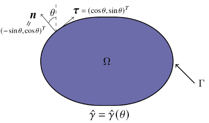
As shown in Fig. 1, let be a closed curve in two dimensions (2D) associated with a given anisotropic surface energy , where represents the angle between the vertical axis and unit outward normal vector . It should be noted that the anisotropy can also be viewed as a function of the normal vector [30, 31, 43]. While is equivalent to by the one-to-one correspondence , the formulation is often more convenient and straightforward in 2D.
Suppose is represented by , where denotes the arc-length parameter, and represents the time. The motion of under anisotropic surface diffusion is governed by the following geometric flow [18, 35]:
| (1.1) |
where is the weighted curvature (or chemical potential) defined as
| (1.2) |
with being the curvature.
The anisotropic surface diffusion (1.1) is a fourth-order and highly nonlinear geometric flow, which possesses two major geometric properties, i.e., the area conservation and the energy dissipation. Let be the area of the region enclosed by , and be the total surface free energy, which are defined as
| (1.3) |
| (1.4) |
which immediately implies the anisotropic surface diffusion (1.1)–(1.2) satisfies the area conservation and energy dissipation, i.e.,
| (1.5) |
When , the weighted curvature reduces to , and it is referred to as isotropic surface energy. If is not a constant function and for all , we classify the surface energy as weakly anisotropic, otherwise, it is termed strongly anisotropic. Typical anisotropic surface energies which are widely employed in materials science include:
-
1.
the -fold anisotropic surface energy [4]
(1.6) where are dimensionless strength constants, is a constant. Note that is weakly anisotropic when , and strongly anisotropic otherwise.
-
2.
the ellipsoidal anisotropic surface energy [44]
(1.7) where are two dimensionless constants satisfying and .
- 3.
- 4.
Many numerical methods have been proposed for simulating the evolution of curves under surface diffusion, including the phase-field method [42, 21, 27, 23], the discontinuous Galerkin method [48], the marker particle method [47, 20] and the parametric finite element method (PFEM) [12, 15, 17, 1]. Among these methods, the energy-stable PFEM (ES-PFEM) by Barrett, Garcke, and Nürnberg [12], also referred to as BGN’s method, achieves the best performance in terms of mesh quality and unconditional energy-stability in the isotropic case. The ES-PFEM has been further extended to other geometric flows, such as the solid-state deweting problem [4, 28, 46], demonstrating its adaptability and robustness. Furthermore, Bao and Zhao have recently developed a structure-preserving PFEM (SP-PFEM) [11, 2, 3], which can preserve the enclosed mass at the fully-discretized level while also maintaining the unconditional energy stability. Extending these PFEMs to anisotropic surface diffusion is a major focus of recent research in surface diffusion. While BGN successfully adapted their methods to a specific Riemannian metric form [14, 16], designing a SP-PFEM for anisotropic surface diffusion with arbitrary anisotropies remains challenging.
Lately, based on the formulation, Li and Bao introduced a surface energy matrix and extended the ES-PFEM from the isotropic cases to the anisotropic cases [33]. Due to the absence of a stabilizing term, their method requires a certain restrictive condition to ensure the energy stability. Subsequently, Bao, Jiang, and Li incorporated a stabilizing function within the formulation. They constructed a symmetric surface energy matrix and proposed a symmetrized SP-PFEM for the anisotropic surface diffusion in [5, 8]. The symmetrized SP-PFEM with the stabilizing function works effectively for symmetric surface energy distributions (i.e., ) to maintain the geometric properties. However, there are different anisotropic surface energies which are not symmetrically distributed or do not satisfy the specific condition, such as the -fold anisotropic surface energy (1.6) [4, 46]. Very recently, based on the formulation, Bao and Li introduced a novel surface energy matrix and established a comprehensive analytical framework to demonstrate the unconditional energy stability of the proposed SP-PFEM [7, 9]. Based on this framework, they successfully reduced the requirement for the anisotropy to .
However, the critical situation was not addressed in their analytical framework. This is because their framework relies on an estimate of the gradient of . The challenge comes from being a function defined on the unit sphere , which makes its gradient complicated to analyze. In contrast, the formulation, defined on , possesses a simpler derivative and thus allows for a better analysis of the critical situation . Therefore, inspired by their analytical framework, we adopt the formulation to further investigate the critical situation.
The main objective of this paper is to propose a structure-preserving stabilized parametric finite element method (SPFEM) for simulating surface diffusion (1.1) with the surface energy under very mild conditions as
-
1.
-
2.
, when .
Compared to the formulation, the formulation has the following advantages:
-
1.
it is more intuitive and has a simpler form in practical applications;
-
2.
it enables a reduction in the regularity requirement for the anisotropy from to globally and piecewise ;
-
3.
it allows for a more convenient discussion of critical situations as for some in 2D.
The remainder of this paper is organized as follows: In section 2, we introduce a stabilized surface energy matrix and propose a new conservative formulation for anisotropic surface diffusion. In section 3, we present a novel weak formulation based on the conservative form, introduce its spatial semi-discretization, and propose a full discretization by SPFEM. In section 4, we analyze the structure-preserving properties of the proposed scheme, i.e., area conservation and unconditional energy stability, and develop a comprehensive framework for energy stability. It starts from defining a minimal stabilizing function , then we obtain the main result through a local energy estimate under the assumption that is well-defined. The existence of is further demonstrated in section 5. In section 6, we extend the SPFEM for simulating solid-state dewetting of thin films under anisotropic surface diffusion and contact line migration. Extensive numerical results are provided in section 7 to demonstrate the efficiency, accuracy and structure-preserving properties of the proposed SPFEM. Finally, we conclude in section 8.
2 A conservative formulation
In this section, we propose a novel formulation with stabilization for (1.1) and derive a conservative form by introducing a stabilized surface energy matrix.
Applying the geometric identity [34], the anisotropic surface diffusion equations (1.1)–(1.2) can be reformulated into
| (2.1a) | |||
| (2.1b) | |||
where is the length of .
For a vector , we denote as its perpendicular vector which is the clockwise rotation of by , i.e.
| (2.2) |
Then the tangent vector , and unit normal vector can be written as . And the tangent vector can also be given by .
Theorem 2.1.
For the weighted curvature given in (1.2), the following identity holds:
| (2.3) |
with
| (2.4) |
is a non-negative stabilizing function.
Proof.
Noticing
| (2.5) |
therefore
| (2.6) |
which implies that
| (2.7) |
By the geometric identity and , we obtain
| (2.8) |
| (2.9) | ||||
and
| (2.10) | ||||
Note that , thus vanishes. Combining (2.1b), (2.9) and (2.10), we have
| (2.11) | ||||
On the other hand, by (2.5), we have
| (2.12) |
consequently
| (2.13) | ||||
where is the identity matrix. Substituting (2.13) into (2.11), the desired equality (2.3) is obtained. ∎
Applying (2.3), the governing geometric PDE (2.1) for anisotropic surface diffusion can be reformulated as the following conservative form
| (2.14a) | |||
| (2.14b) | |||
Remark 2.1.
If we take the stabilizing term in (2.4), then collapses to the surface energy matrix proposed in [33]. Moreover, with the adoption of the formulation, we can define the corresponding stabilizing function by the one-to-one correspondence , and the stabilizing term is simplified to . Consequently, is transformed into the surface energy matrix in [7].
Remark 2.2.
At the continuous level, makes no contribution, as . Thus, the conservative form (2.14) and the original form (2.1) are equivalent. At the discrete level, however, serves as a stabilizing term, which relaxes the energy stability conditions for the anisotropy . For example, surface matrix in [33] (absent the stabilizing term) only guarantees energy stability for specific cases of weakly anisotropic surface energy. In contrast, with this stabilizing term, this formulation can be applied to more general anisotropies, see (3.36)
3 A SPFEM for anisotropic surface diffusion
In this section, we first develop a novel weak formulation based on the conservative form (2.14) and present the spatial semi-discretization of this weak formulation. After that, a structure-preserving SPFEM is proposed by adapting the implicit-explicit Euler method in time, which preserves area conservation and energy dissipation at the discrete level.
3.1 Weak formulation
In order to derive a weak formulation of equation (2.14), we introduce a time-independent variable which parameterizes over a fixed domain as
| (3.1) |
The arc-length parameter can thus be computed by . (We do not distinguish and if there’s no misunderstanding.)
Introduce the following functional space with respect to the evolution curve as
| (3.2) |
equipped with the -inner product
| (3.3) |
for any scalar (or vector) functions. The Sobolev spaces are defined as
| (3.4a) | ||||
| (3.4b) | ||||
Extensions of above definitions to the functions in and are straightforward.
By multiplying the equation (2.14a) by a test function , integrating over , and applying integration by parts, we obtain
| (3.5) |
Similarly, by taking the dot product of equation (2.14b) with a test function and integrating by parts, we have
| (3.6) | ||||
Combining (3.5) and (3.6), we propose a new weak formulation for (2.14) as follows: Given an initial closed curve , find the solution , such that:
| (3.7a) | ||||
| (3.7b) | ||||
It can be demonstrated that the weak formulation (3.7) maintains two geometric properties, namely, area conservation and energy dissipation.
Proposition 3.1 (area conservation and energy dissipation).
Suppose is given by the solution of the weak formulation (3.7), denote as the enclosed area and as the total energy of the closed evolving curve , respectively, which are formally given by
| (3.8) |
Then we have
| (3.9) |
More precisely,
| (3.10) |
To prove the above theorem, we first introduce the following transport lemma:
Lemma 3.1.
Suppose is a two-dimensional piecewise curve parameterized by , is a differentiable function, then
| (3.11) |
Proof.
Since , then
| (3.12) | ||||
thus
| (3.13) | ||||
∎
Now the proof of Proposition 3.1 is ready to be presented:
Proof.
Denote the region enclosed by as . For the area conservation, by the Reynolds’ transport theorem [38] and taking in (3.7a),
| (3.14) | ||||
For the energy dissipation part, by Lemma 3.1, we have
| (3.15) | ||||
On the other hand, by using (3.12), we can simplify as
| (3.16) | ||||
This, together with the fact , yields that
| (3.17) |
Therefore,
| (3.18) |
Since , then
| (3.19) | ||||
which leads to
| (3.20) |
Therefore, by taking and in (3.7a) and (3.7b), respectively, we have
| (3.21) | ||||
∎
3.2 A semi-discretization in space
To obtain the spatial discretization, let be a positive integer and be the mesh size, grid points , sub-intervals for and the uniform partition . The closed curve is approximated by the polygonal curve satisfying .
The polygon is composed of ordered line segments , i.e.
| (3.22) |
And we always assume that for all .
By using , the discrete geometric quantities such as the unit tangential vector , the outward unit normal vector and the inclination angle can be computed on each segment as:
| (3.23) |
and
| (3.24) |
We introduce the finite element subspaces
| (3.25a) | |||
| (3.25b) | |||
where is the set of polynomials defined on of degree . For , the mass-lumped inner product with respect to is defined as
| (3.26) |
where . And the discretized differential operator for is defined as
| (3.27) |
The above definitions also hold true for vector-valued functions.
We now propose the spatial semi-discretization for (3.7) as follows: Let be the approximations of , respectively, for , find the solution such that
| (3.28a) | |||
| (3.28b) | |||
where
| (3.29) |
Denote the enclosed area and the free energy of the polygonal curve as and , respectively, which are given by
| (3.30a) | |||
| (3.30b) | |||
where .
Following similar steps in Proposition 3.1, it can be proved that the two geometric properties for the semi-discretization (3.28) still preserves:
Proposition 3.2 (area conservation and energy dissipation).
Suppose is given by the solution of (3.28), then we have
| (3.31) |
3.3 A structure-preserving SPFEM discretization
Let be the uniform time step. Denoting the approximation of at as where . Then the definitions of the mass lumped inner product , the unit tangential vector , the unit outward normal vector , and the inclination angle with respect to can be given in a similar approach.
Following the ideas in [11, 32, 5, 3] to design an SP-PFEM for surface diffusion, we utilize the explicit-implicit Euler method in time. The derived fully-implicit structure-preserving discretization of SPFEM for the anisotropic surface diffusion (2.1) is expressed as follows:
Suppose the initial approximation is given by . For any , find the solution such that
| (3.32a) | |||
| (3.32b) | |||
where
| (3.33) |
and
| (3.34) |
Remark 3.1.
The above scheme is weakly implicit, as the integral domain is explicitly chosen and each equation contains only one non-linear term. The nonlinear term is a polynomial function of degree with respect to the components of and , thus it can be efficiently and accurately solved by the Newton’s iterative method similar to [11].
Remark 3.2.
The choice of is crucial for maintaining the area conservation. The scheme becomes semi-implicit if is replaced by , and only the energy dissipation property is preserved.
3.4 Main results
Denote the enclosed area and the free energy of the polygon as and , respectively, which are given by
| (3.35a) | ||||
| (3.35b) | ||||
In practical applications, it’s common to encounter situations where lacks high regularity. In the following sections, we always assume that is globally and piecewise on .
We thus introduce the following energy stable conditions on :
Definition 3.1 (energy stable condition).
Suppose is globally and piecewise , the energy stable conditions on are given as follows:
| (3.36a) | |||
| (3.36b) | |||
The main result of this work is the following structure-preserving property of the SPFEM (3.32):
Theorem 3.2 (structure-preserving).
The proof of area conservation part is analogous to [11, Theorem 2.1], we omit here for brevity. And the energy dissipation will be established in the next section.
Remark 3.3.
Remark 3.4.
4 Unconditionally energy stability of the SPFEM
The key point in proving energy dissipation of (3.32) is to establish an energy estimate akin to
| (4.1) |
for controlling the energy difference between two subsequent time steps with the surface energy matrix . To achieve desired inequality, we need a local version of the estimate, which is formulated by the following lemma:
Lemma 4.1 (local energy estimate).
Suppose are two non-zero vectors in . Let and be the corresponding unit normal vectors. Then for sufficiently large , the following inequality holds
| (4.2) |
Remark 4.1.
4.1 The minimal stabilizing function and its properties
To prove the local energy estimate (4.2), the following two auxiliary functions are introduced as:
| (4.3a) | |||
| (4.3b) | |||
With the help of , we present the definition of minimal stabilizing function as follows:
| (4.4) |
The following theorem guarantees the existence of :
Theorem 4.3.
Once the is given, the minimal stabilizing function is determined, inducing a mapping from to . Moreover, this mapping is sublinear, i.e., it is positive homogeneity and subadditivity.
Lemma 4.2 (positive homogeneity and subadditivity).
Let for denote anisotropies satisfying (3.36), each corresponding to its minimal stabilizing functions . Then, we have
-
1.
if for a given positive number , then ;
-
2.
if , then .
The proof is similar to [5, Lemma 4.4], we omit here for brevity.
4.2 Proof of the local energy estimate
Proof.
Applying the definitions of in (2.4), noting that
| (4.5) |
then we have
| (4.6) | ||||
and
| (4.7) | ||||
Recall the definitions of in (4.3), we have
| (4.8a) | ||||
| (4.8b) | ||||
with .
Substituting (4.8a), (4.8b) into the local energy estimate (4.2), we have
| (4.9) | ||||
thus the local energy estimate (4.2) is equivalent to
| (4.10) |
i.e.
| (4.11) |
By the definition (4.4) of , we have for any , thus (4.11) holds true. By Theorem 4.3, the minimal stabilizing function is well-defined, therefore we can choose sufficiently large such that the intended local energy estimate (4.2) is validated. ∎
4.3 Proof of the main result
5 Existence of the minimal stabilizing function
In this section, we present a proof of the existence of the minimal stabilizing function corresponding to that satisfies the energy stable condition in (3.36).
Before formally commencing our proof, we first need the following two technical lemmas:
Lemma 5.1.
For a globally and piecewise anisotropy , there exists an open neighborhood of and a positive constant such that for any , we have .
Proof.
Since is globally and piecewise , there exists a such that is -times continuously differentiable on both and .
Applying the mean value theorem to and , we deduce that for , there exists a between and such that
| (5.2) |
Again, by the mean value theorem, there exist between such that
| (5.3a) | ||||
| (5.3b) | ||||
Substituting (5.2) and (5.3) into , we have
| (5.4) | ||||
Thus,
| (5.5) | ||||
Since , then for any ,
| (5.6) | ||||
Noting that for any , we have , therefore,
| (5.7) | ||||
Thus there exists a positive constant , for , . ∎
Lemma 5.2.
Suppose satisfying (3.36). There exists an open neighborhood of with a positive such that for any , .
Proof.
-
1.
If for any , then
(5.8) Thus, by the continuity of , there exists an open neighborhood of such that .
-
2.
If and at . Since function , it attends its maximum at , thus
(5.9) i.e., .
Similar to derivations of (5.2), according to the mean value theorem, we know that there exists positive number and a neighborhood . Such that for any , there exists a between and satisfying
(5.10) Again, by the mean value theorem, we know that there exists a between ,
(5.11) By substituting (5.10) and (5.11) into , we have
(5.12) Thus,
(5.13) Given that , we can deduce that
(5.14) Noting that for any , we have since . Therefore,
(5.15) Therefore, there exists a positive constant , such that for , we have .
∎
With the help of above two lemmas, Theorem 4.3 can now be proven:
Proof.
(Existence of the minimal stabilizing function)
-
1.
For any , i.e. , there exists an open neighborhood of such that has a strict positive lower bound in , i.e. there exists a constant such that , then we have
(5.16) Thus there positive exists a constant , for any , .
-
2.
For , by Lemma 5.1, there exists an open neighborhood of and a positive constant such that for any , .
-
3.
For , by Lemma 5.2, there also exists an open neighborhood of with a positive constant such that for any , .
Since is compact and forms an open cover of , by the open cover theorem, one can select a finite subcover , then for , we have
| (5.17) |
Which implies . ∎
6 Extension to solid-state dewetting
In this section, we extend the conservative formulation (2.14) and its SPFEM (3.32) for a closed curve under anisotropic surface diffusion to solid-state dewetting in materials science [4, 28, 46].
6.1 Sharp interface model and a stabilized formulation
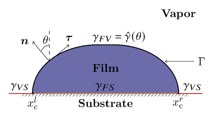
As shown in Fig. 2, the solid-state dewetting problem in 2D is described as evolution of an open curve under anisotropic surface diffusion and contact line migration. Here, and are the arc-length parameter and time, respectively, and represents the total length of . As it was derived in the literature [4, 28, 46], a dimensionless sharp-interface model for simulating solid-state dewetting of thin films with weakly anisotropic surface energy can be formulated as: satisfying anisotropic surface diffusion (1.1)–(1.2) with following boundary conditions
-
1.
contact point condition
(6.1) -
2.
relaxed contact angle condition
(6.2) -
3.
zero-mass flux condition
(6.3)
where are the left and right contact points, are the contact angles at each contact points, respectively. is defined as
| (6.4) |
with and be the isotropic Young contact angle. denotes the contact line mobility [4, 28, 46].
6.2 A stabilized weak formulation
Suppose is parameterized by a time-independent variable over a fixed domain , i.e.
| (6.6) |
thus the arc-length parameter can be given as . (Again, we do not distinguish and .)
Introducing the following functional spaces as
| (6.7) |
Following similar derivations as in Section 3, we present the new variational formulation for (6.5) with boundary conditions (6.1)–(6.3) as follows: Given an initial open curve , find the solution such that
| (6.8a) | ||||
| (6.8b) | ||||
The area enclosed by and the substrate and the total energy are defined as
| (6.9) |
Similar to the closed curve case, the weak formulation (6.8) still preserves area conservation and energy dissipation.
Proposition 6.1 (area conservation and energy dissipation).
The proof is similar to Proposition 3.1, we omit the details here for brevity.
6.3 A SPFEM and its proprieties
Introducing the finite element spaces
| (6.12) |
The semi-discretization in space of (6.8) and its area conservation and energy dissipation properties are similar to Section 3, we omit the details here for brevity.
Let be the uniform time step, denotes the approximation of at as where . Then the structure-preserving discretization of SPFEM for solid-state dewetting (6.5) can be stated as: Suppose the initial approximation is given by . For any , find the solution , such that
| (6.13a) | ||||
| (6.13b) | ||||
satisfying . The definition of is similar to (3.34).
Denote the area enclosed by the open polygonal curve and the substrate and the total surface energy as
| (6.14a) | ||||
| (6.14b) | ||||
Then for the SPFEM (6.13), we have following result on its structure preservation.
Theorem 6.4 (structure-preserving).
7 Numerical results
In this section, we report numerical experiments for the proposed SPFEM (3.32) and (6.13) for time evolutions of closed curves and open curves, respectively. Extensive results are provided to illustrate their efficiency, accuracy, area conservation and unconditional energy stability.
In the numerical tests, following typical anisotropic surface energies are considered in the simulations:
-
1.
Case I: with . It is weakly anisotropic when and strongly anisotropic otherwise;
-
2.
Case II: with .
To compute the minimal stabilizing function , we solve the optimization problem (4.4) for 20 uniformly distributed points in and do linear interpolation for the intermediate points.
To verify the quadratic convergence rate in space and linear convergence rate in time, the time step is always chosen as except it is stated otherwise. The manifold distance [50, 33]
| (7.1) |
is employed to measure the distance between two closed curves , where are the regions enclosed by and represents the area of . Suppose is the numerical approximation of , thus the numerical error is defined as
| (7.2) |
In the Newton’s iteration, the tolerance value is set to be .
To test the mesh quality, the energy stability and area conservation numerically, we introduce the following indicators: the weighted mesh ratio
| (7.3) |
the normalized area loss and the normalized energy for closed curves:
| (7.4) |
and for open curves:
| (7.5) |
In the following numerical tests, the initial shapes are chosen as a complete and a half ellipse with major axis and minor axis for closed curves and open curves, respectively, unless stated otherwise. The exact solution is approximated by choosing with a small mesh size and a time step in (3.32). For solid-state dewetting problems, we always choose the contact line mobility .
7.1 Results for closed curves
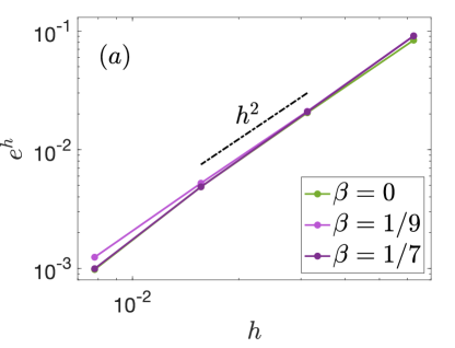
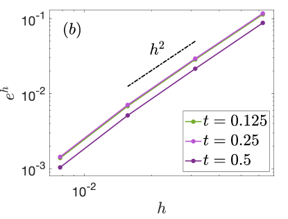
Fig. 3 plots the convergence rates of the proposed SPFEM (3.32) for: (a) the -fold anisotropy with different anisotropic strengths under a fixed time ; (b) the ellipsoidal anisotropy at different times. It clearly demonstrates that the second-order spatial convergence remains consistent regardless of anisotropies and computational times, suggesting a high level of robustness in the convergence rate.
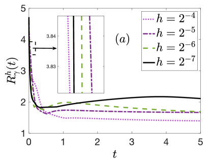
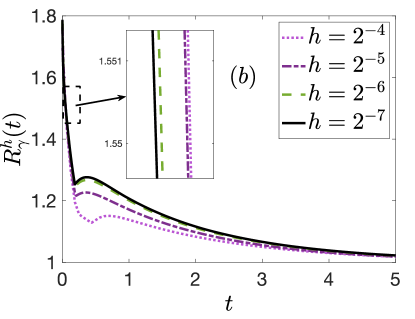
Fig. 4 exhibits that the weighted mesh ratio converge to constants as . This suggests an asymptotic quasi-uniform mesh distribution of the proposed SPFEM (3.32).
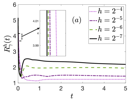
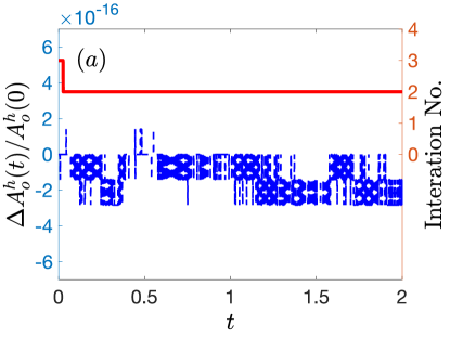
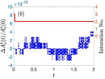
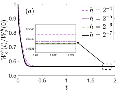
The time evolutions of the normalized area loss , the number of the Newton’s iteration with are given in Fig. 5. And the normalized energy with different are summarized in Fig. 6.
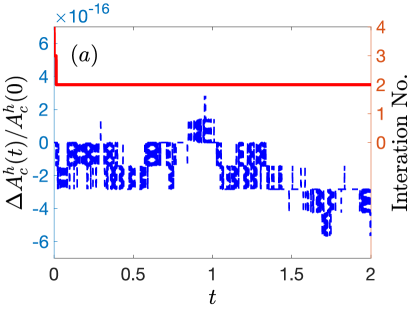
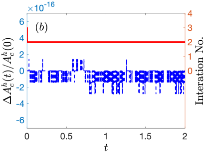
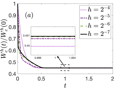
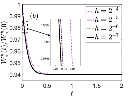
The observation from Fig. 5–Fig. 6 reveals that:
-
1.
The normalized area loss is at , aligns closely with the order of the round-off error (cf. Fig. 5). This observation affirms the practical preservation of area in simulations.
- 2.
-
3.
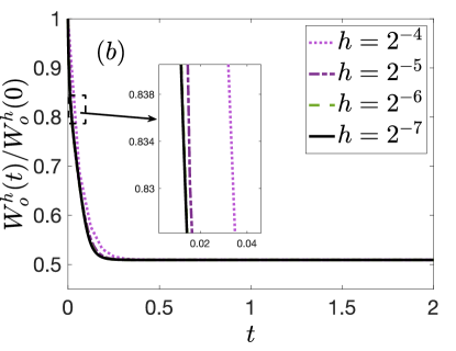
The normalized energy is monotonically decreasing when satisfies the energy stable conditions (3.36) in Definition 3.1 (cf. Fig. 6). Results in Fig. 6 (a) shows that the proposed SPFEM (3.32) still preserves good energy stability properties when takes its maximum value of in Remark 3.3. And results in Fig. 6 (b) indicate that, unlike the ES-PFEM in [33], the SPFEM remains unconditionally energy stable when as stated in Remark 3.4.
7.2 Results for open curves in solid-state dewetting
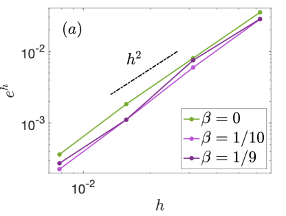
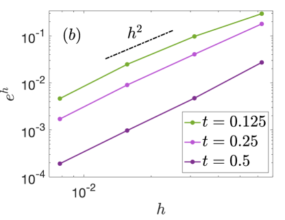
Fig. 7 plots the computation errors of the proposed SPFEM (6.13) for: (a) the -fold anisotropy with different anisotropic strengths under a fixed time ; (b) the ellipsoidal anisotropy at different times. The results verify the quadratic convergence rate for the proposed SPFEM (6.13).

In Fig. 8, the weighted mesh ratios tend to constants as , showing that the SPFEM (6.13) still possesses the asymptotic quasi-uniform distribution.
Time evolutions of the normalized area loss , the number of the Newton’s iteration with are presented in Fig. 9. And the normalized energy with different are illustrated in Fig. 10.
7.3 Application for morphological evolutions
Finally we apply the proposed SPFEMs (3.32) and (6.13) to simulate the morphological evolutions under the anisotropic surface diffusion. Results for both closed curves and open curves in solid-state dewetting problems are provided.
The morphological evolutions from the initial shapes to their numerical equilibriums are presented in Fig. 11–Fig. 13. For closed curve cases, the initial shape is an ellipse with major axis and minor axis , while for open curve cases, it is an open rectangle.
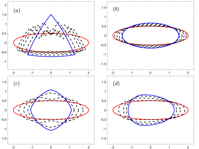
Fig. 11 plots the morphological evolutions of an ellipse with major axis and minor axis under anisotropic surface diffusion with four different surface energies: (a) anisotropy in Case I with , which attends the maximum value in Remark 3.3; (b) anisotropy in Case II with ; (c) the -fold anisotropy [4]; and (d) with [19].
Results in Fig. 11 (b) and Fig. 11 (c) show that, compared to the ES-PFEM in [33], the proposed SPFEM (3.32) demonstrates a better performance over a broader range of parameters during evolutions. Fig. 11 (d) indicates that the SPFEM (3.32) also works well for a globally and piecewise anisotropy.

And Fig. 12 illustrates the morphological evolutions under anisotropic surface diffusion with different surface energies for a four-fold star shape curve
| (7.6) |
and an ellipse (with major axis and minor axis ) rotated counterclockwise by .
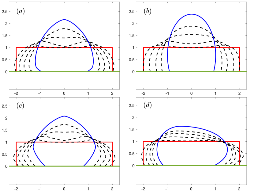
In Fig. 13, we display the morphological evolutions from an open rectangular curve to their equilibriums shapes with different surface energies: (a) anisotropy in Case I with ; (b) anisotropy in Case II with ; (c) the -fold anisotropy ; (d) with .
8 Conclusions
We propose a structure-preserving stabilized parametric finite element method (SPFEM) for the anisotropic surface diffusion. This method is subject to mild conditions on , and works effectively for closed curves and open curves with contact line migration in solid-state dewetting. By introducing a new stabilized surface energy matrix, we obtain a conservative form and its weak formulation for anisotropic surface diffusion. Based on this weak formulation, a novel SPFEM is proposed by utilizing the PFEM for spatial discretization and the implicit-explicit Euler method for temporal discretization. To analyze the unconditional energy stability, we extend the framework proposed by Bao and Li to the formulation. This approach starts by defining the minimal stabilizing function, proving its existence, results in a local energy estimate, and subsequently establishes unconditional energy stability. Due to the very mild requirements on the surface energy , the methods are able to simulate over a broader range of anisotropies for both closed curves and open curves. Moreover, the SPFEMs are applicable for the globally and piecewise anisotropy as well, which is a capability not possessed by other PFEMs.
CRediT authorship contribution statement
Yulin Zhang: Conceptualization, Methodology, Software, Investigation, Writing - Original Draft.
Yifei Li: Project administration, Supervision, Writing - Review & Editing.
Wenjun Ying: Supervision, Writing - Review & Editing.
Declaration of competing interest
The authors declare that they have no known competing financial interests or personal relationships that could have appeared to influence the work reported in this paper.
Acknowledgement
We would like to specially thank Professor Weizhu Bao for his valuable suggestions and comments. The work of Zhang was partially supported by the State Scholarship Fund (No.202306230346) by the Chinese Scholar Council (CSC) and the Zhiyuan Honors Program for Graduate Students of Shanghai Jiao Tong University (No.021071910051). The work of Li was funded by the Ministry of Education of Singapore under its AcRF Tier 2 funding MOE-T2EP20122-0002 (A-8000962-00-00). Part of the work was done when the authors were visiting the Institute of Mathematical Science at the National University of Singapore in 2024.
References
- [1] Bänsch, E., Morin, P., Nochetto, R.: A finite element method for surface diffusion: the parametric case. J. Comput. Phys. 203, 321-343 (2005)
- [2] Bao, W., Garcke, H., Nürnberg, R., Zhao, Q. Volume-preserving parametric finite element methods for axisymmetric geometric evolution equations. J. Comput. Phys. 460, 111180 (2022)
- [3] Bao, W., Garcke, H., Nürnberg, R., Zhao, Q.: A structure-preserving finite element approximation of surface diffusion for curve networks and surface clusters. Numer. Methods Partial Differ. Eq. 39, 759-794 (2023)
- [4] Bao, W., Jiang, W., Wang, Y., Zhao, Q.: A parametric finite element method for solid-state dewetting problems with anisotropic surface energies. J. Comput. Phys. 330, 380-400 (2017)
- [5] Bao, W., Jiang, W., Li, Y.: A symmetrized parametric finite element method for anisotropic surface diffusion of closed curves. SIAM J. Numer. Anal. 61, 617-641 (2023)
- [6] Bao, W., Jiang, W., Srolovitz, D., Wang, Y.: Stable equilibria of anisotropic particles on substrates: a generalized Winterbottom construction. SIAM J. Appl. Math. 77, 2093-2118 (2017)
- [7] Bao, W., Li, Y.: A structure-preserving parametric finite element method for geometric flows with anisotropic surface energy. Numer. Math. online, (2024)
- [8] Bao, W., Li, Y.: A symmetrized parametric finite element method for anisotropic surface diffusion in three dimensions. SIAM J. Sci. Comput. 45, A1438-A1461 (2023)
- [9] Bao, W., Li, Y.: A unified structure-preserving parametric finite element method for anisotropic surface diffusion. Preprint ArXiv:2401.00207. (2023)
- [10] Bao, W., Zhao, Q.: An energy-stable parametric finite element method for simulating solid-state dewetting problems in three dimensions. J. Comp. Math. 41, 771-796 (2023)
- [11] Bao, W., Zhao, Q.: A structure-preserving parametric finite element method for surface diffusion. SIAM J. Numer. Anal. 59, 2775-2799 (2021)
- [12] Barrett, J., Garcke, H., Nürnberg, R.: A parametric finite element method for fourth order geometric evolution equations. J. Comput. Phys. 222, 441-467 (2007)
- [13] Barrett, J., Garcke, H., Nürnberg, R.: On the variational approximation of combined second and fourth order geometric evolution equations. SIAM J. Sci. Comput. 29, 1006-1041 (2007)
- [14] Barrett, J., Garcke, H., Nürnberg, R.: Numerical approximation of anisotropic geometric evolution equations in the plane. IMA J. Numer. Anal. 28, 292-330 (2008)
- [15] Barrett, J., Garcke, H., Nürnberg, R.: On the parametric finite element approximation of evolving hypersurfaces in R3. J. Comput. Phys. 227, 4281-4307 (2008)
- [16] Barrett, J., Garcke, H., Nürnberg, R.: A variational formulation of anisotropic geometric evolution equations in higher dimensions. Numer. Math. 109, 1-44 (2008)
- [17] Barrett, J., Garcke, H., Nürnberg, R.: Parametric finite element approximations of curvature-driven interface evolutions. Handb. Numer. Anal. 21 pp. 275-423 (2020)
- [18] Cahn, J., Taylor, J.: Overview no. 113 surface motion by surface diffusion. Acta Metall. Mater. 42, 1045-1063 (1994)
- [19] Deckelnick, K., Dziuk, G., Elliott, C.: Computation of geometric partial differential equations and mean curvature flow. Acta Numer. 14 pp. 139-232 (2005)
- [20] Du, P., Khenner, M., Wong, H.: A tangent-plane marker-particle method for the computation of three-dimensional solid surfaces evolving by surface diffusion on a substrate. J. Comput. Phys. 229, 813-827 (2010)
- [21] Du, Q., Feng, X.: The phase field method for geometric moving interfaces and their numerical approximations. Handb. Numer. Anal. 21, 425-508 (2020)
- [22] Fonseca, I., Pratelli, A., Zwicknagl, B.: Shapes of epitaxially grown quantum dots. Arch. Ration. Mech. Anal. 214 pp. 359-401 (2014)
- [23] Garcke, H., Knopf, P., Nürnberg, R., Zhao, Q.: A diffuse-interface approach for solid-state dewetting with anisotropic surface energies. J. Nonl. Sci. 33, 34 (2023)
- [24] Gilmer, G., Bennema, P.: Simulation of crystal growth with surface diffusion. J. Appl. Phys. 43, 1347-1360 (1972)
- [25] Gomer, R.: Diffusion of adsorbates on metal surfaces. Rep. Progr. Phys. 53, 917 (1990)
- [26] Gurtin, M., Jabbour, M.: Interface Evolution in Three Dimensions with Curvature-Dependent Energy and Surface Diffusion: Interface-Controlled Evolution, Phase Transitions, Epitaxial Growth of Elastic Films. Arch. Ration. Mech. Anal. 163 pp. 171-208 (2002)
- [27] Jiang, W., Bao, W., Thompson, C., Srolovitz, D.: Phase field approach for simulating solid-state dewetting problems. Acta Mater. 60, 5578-5592 (2012)
- [28] Jiang, W., Wang, Y., Zhao, Q., Srolovitz, D., Bao, W.: Solid-state dewetting and island morphologies in strongly anisotropic materials. Scr. Mater. 115, 123-127 (2016)
- [29] Jiang, W., Wang, Y., Srolovitz, D., Bao, W.: Solid-state dewetting on curved substrates. Phys. Rev. Mater. 2, 113401 (2018)
- [30] Jiang, W., Zhao, Q.: Sharp-interface approach for simulating solid-state dewetting in two dimensions: A Cahn-Hoffman -vector formulation. Phys. D: Nonl. Phen. 390, 69-83 (2019)
- [31] Jiang, W., Zhao, Q., Bao, W.: Sharp-interface model for simulating solid-state dewetting in three dimensions. SIAM J. Appl. Math. 80, 1654-1677 (2020)
- [32] Jiang, W., Li, B.: A perimeter-decreasing and area-conserving algorithm for surface diffusion flow of curves. J. Comput. Phys. 443, 110531 (2021)
- [33] Li, Y., Bao, W.: An energy-stable parametric finite element method for anisotropic surface diffusion. J. Comput. Phys. 446, 110658 (2021)
- [34] Mantegazza, C.: Lecture notes on mean curvature flow. (Springer Science & Business Media, 2011)
- [35] Mullins, W.: Theory of thermal grooving. J. Appl. Phys. 28, 333-339 (1957)
- [36] Oura, K., Lifshits, V., Saranin, A., Zotov, A. Katayama, M.: Surface science: an introduction. (Springer Science & Business Media, 2013)
- [37] Randolph, S., Fowlkes, J., Melechko, A., Klein, K., Meyer, H., Simpson, M., Rack, P.: Controlling thin film structure for the dewetting of catalyst nanoparticle arrays for subsequent carbon nanofiber growth. Nanotech. 18, 465304 (2007)
- [38] Reynolds, O.: Papers on mechanical and physical subjects. (CUP Arch., 1983)
- [39] Shen, H., Nutt, S., Hull, D.: Direct observation and measurement of fiber architecture in short fiber-polymer composite foam through micro-CT imaging. Compos. Sci. Technol. 64, 2113-2120 (2004)
- [40] Shustorovich, E.: Metal-surface reaction energetics. Theory and application to heterogeneous catalysis, chemisorption, and surface diffusion. (New York; VCH Publ. Inc.,1991)
- [41] Srolovitz, D., Safran, S.: Capillary instabilities in thin films. II. Kinetics. J. Appl. Phys. 60, 255-260 (1986)
- [42] Tang, T., Qiao, Z.: Efficient numerical methods for phase-field equations (in Chinese). Sci. China Series A-Math. (in Chinese) 50, 1-20 (2020)
- [43] Taylor, J.: II-mean curvature and weighted mean curvature. Acta Metall. Mater. 40, 1475-1485 (1992)
- [44] Taylor, J., Cahn, J.: Linking anisotropic sharp and diffuse surface motion laws via gradient flows. J. Stat. Phys. 77, 183-197 (1994)
- [45] Thompson, C.: Solid-state dewetting of thin films. Annu. Rev. Mater. Res. 42, 399-434 (2012)
- [46] Wang, Y., Jiang, W., Bao, W., Srolovitz, D.: Sharp interface model for solid-state dewetting problems with weakly anisotropic surface energies. Phys. Rev. B 91, 045303 (2015)
- [47] Wong, H., Voorhees, P., Miksis, M., Davis, S.: Periodic mass shedding of a retracting solid film step. Acta Mater. 48, 1719-1728 (2000)
- [48] Xu, Y., Shu, C.: Local discontinuous Galerkin method for surface diffusion and Willmore flow of graphs. J. Sci. Comput. 40, 375-390 (2009)
- [49] Ye, J., Thompson, C.: Mechanisms of complex morphological evolution during solid-state dewetting of single-crystal nickel thin films. Appl. Phys. Lett. 97 (2010)
- [50] Zhao, Q., Jiang, W., Bao, W.: An energy-stable parametric finite element method for simulating solid-state dewetting. IMA J. Numer. Anal. 41, 2026-2055 (2021)