Asymptotics of resampling without replacement in robust and logistic regression

Abstract

This paper studies the asymptotics of resampling without replacement in the proportional regime where dimension $p$ and sample size $n$ are of the same order. For a given dataset $(\bm{X},\bm{y})\in\mathbb{R}^{n\times p}\times\mathbb{R}^{n}$ and fixed subsample ratio $q\in(0,1)$, the practitioner samples independently of $(\bm{X},\bm{y})$ iid subsets $I_{1},...,I_{M}$ of $\{1,...,n\}$ of size $qn$ and trains estimators $\hat{\bm{b}}(I_{1}),...,\hat{\bm{b}}(I_{M})$ on the corresponding subsets of rows of $(\bm{X},\bm{y})$. Understanding the performance of the bagged estimate $\bar{\bm{b}}=\frac{1}{M}\sum_{m=1}^{M}\hat{\bm{b}}(I_{1}),...,\hat{\bm{b}}(I_{M})$, for instance its squared error, requires us to understand correlations between two distinct $\hat{\bm{b}}(I_{m})$ and $\hat{\bm{b}}(I_{m^{\prime}})$ trained on different subsets $I_{m}$ and $I_{m^{\prime}}$.

In robust linear regression and logistic regression, we characterize the limit in probability of the correlation between two estimates trained on different subsets of the data. The limit is characterized as the unique solution of a simple nonlinear equation. We further provide data-driven estimators that are consistent for estimating this limit. These estimators of the limiting correlation allow us to estimate the squared error of the bagged estimate $\bar{\bm{b}}$, and for instance perform parameter tuning to choose the optimal subsample ratio $q$. As a by-product of the proof argument, we obtain the limiting distribution of the bivariate pair $(\bm{x}_{i}^{T}\hat{\bm{b}}(I_{m}),\bm{x}_{i}^{T}\hat{\bm{b}}(I_{m^{\prime}}))$ for observations $i\in I_{m}\cap I_{m^{\prime}}$, i.e., for observations used to train both estimates.

1 Introduction

This paper studies the performance of bagging estimators trained on subsampled, overlapping datasets in the context robust linear regression and logistic regression.

1.1 M-estimation in the proportional regime

We consider an M-estimation problem in the proportional regime where sample size $n$ and dimension $p$ are of the same order: Throughout the paper, $\delta>1$ is a fixed constant and the ratio

$$n/p=\delta$$ (1.1)

is held fixed as $n,p\to+\infty$ simultaneously. The practitioner collects data $(y_{i},\bm{x}_{i})_{i\in[n]}$ with scalar-valued responses $y_{i}$ and feature vectors $\bm{x}_{i}\in\mathbb{R}^{p}$. For a given subset of observations $I\subset[n]$, an estimator $\hat{\bm{b}}(I)$ is trained on the subset of observations $(y_{i},\bm{x}_{i})_{i\in I}$ using an optimization problem of the form

$$\hat{\bm{b}}(I)=\operatorname*{arg\,min}_{\bm{b}\in\mathbb{R}^{p}}\sum_{i\in I}\ell_{i}(\bm{x}_{i}^{\top}\bm{b})$$ (1.2)

where for each $i\in[n]$, the loss $\ell_{i}(\cdot)$ is convex and depends implicitly on the response $y_{i}$. We will focus on two regression settings: robust linear regression and Generalized Linear Models (GLM), including logistic regression. In robust regression, the response is of the form

$$y_{i}=\bm{x}_{i}^{T}\bm{\beta}^{*}+\varepsilon_{i}$$ (1.3)

for some possibly heavy-tailed noise $\varepsilon_{i}$ independent of $\bm{x}_{i}$. In this case the loss $\ell_{i}$ in (1.2) is given by

$$\ell_{i}(u)=\rho(y_{i}-u)$$ (1.4)

where $\rho$ is a deterministic function, for instance the Huber loss $\rho(u)=\int_{0}^{|u|}\min(1,t)dt$ or its smooth variants, e.g., $\rho(u)=\sqrt{1+u^{2}}$. The asymptotics of the performance of (1.2) with $I=\{1,...,n\}$ and the loss (1.4) in robust regression in the proportional regime (1.1) are now well understood [26, 22, 25, 34] as we will review in Section 2. A typical example of GLM to which our results apply is the case of binary logistic regression, where $\ell_{i}$ in (1.2) is the negative log-likelihood

$$\ell_{i}(u)=\log(1+e^{u})-uy_{i},\qquad y_{i}\in\{0,1\}$$ (1.5)

which is now also well understood for $I=[n]$ in (1.2) [33, 17]. Related results will be reviewed in Section 3. The goal of the present paper is to study the performance of bagging several estimators of the form (1.2) obtained from several subsampled datasets $I_{1},...,I_{M}$.

1.2 Bagging estimators trained on subsampled datasets without replacement

Let $M>0$ be a fixed integer, held fixed as $n,p\to+\infty$. The practitioner then samples $M$ subsets of $[n]$ according to the uniform distribution on all subsets of $[n]$ of size $qn$ for some $q\in(0,1]$, that is,

$$I_{1},...,I_{M}\sim^{\text{iid}}\text{Unif}\{I\subset[n]:|I|=qn\}.$$ (1.6)

Each $I_{m}$ thus samples a subset of $[n]$ of size $qn$ without replacement, and the set of indices $I_{1},...,I_{M}$ are all independent. While the set of indices are independent, the corresponding subsampled datasets

$$(\bm{x}_{i},y_{i})_{i\in I_{m}},\quad\text{ and }\quad(\bm{x}_{i},y_{i})_{i\in I_{m^{\prime}}}$$ (1.7)

are not independent as soon as there is some overlap in the sense $I_{m}\cap I_{m^{\prime}}\neq\emptyset$.

Remark 1.1.

If $I_{m}$ and $I_{m^{\prime}}$ are independent according to (1.6) then $|I_{m}\cap I_{m^{\prime}}|$ follows an hyper-geometric distribution with mean $q^{2}n$, and by Chebychev’s inequality using the explicit formula for the variance of hyper-geometric distributions, $|I_{m}\cap I_{m^{\prime}}|/n\to^{P}q^{2}$ as $n\to+\infty$ while $q$ is held fixed. Thus, not only is the intersection non-empty with high-probability, but it is of order $n$.

The goal of the paper is to understand the performance of bagging the corresponding subsampled estimates: with the notation $\hat{\bm{b}}(I)$ in (1.2) and $I_{1},...,I_{M}$ in (1.6), the practitioner construct the bagged estimate

$$\bar{\bm{b}}=\frac{1}{M}\sum_{m=1}^{M}\hat{\bm{b}}(I_{m}).$$ (1.8)

Related works

Bagging as a generally applicable principle was introduced in [14, 15]. Early analysis of bagging in low-dimensional regimes were performed in [16] among others. In the proportional regime (1.1), LeJeune et al. [28] demonstrated the role of bagging as an implicit regularization technique when the base learners $\hat{\bm{b}}(I_{m})$ are least-squares estimates. Bagging Ridge estimators was studied in [23, 31] who characterized the limit of the squared error of (1.8) using random matrix theory. The implicit regularization power of bagging in the proportional regime is again seen in [31, 23], where it is shown that the optimal risk among Ridge estimates can also be achieved by bagging Ridgeless estimates and optimally choosing the sub sample size. Estimating the risk of a bagged estimate such as (1.8) for regularized least-squares estimates is done in [31, 23, 10]. The risk of bagging random-features estimators, trained on the full dataset but with each base learner having independent weights within the random feature activations, is characterized in [30]. Most recently, [20] studied the limiting equations of several resampling schemes including bootstrap and resampling without replacement, and characterized self-consistent equations for the limiting risk of estimators obtained by minimization of the negative log-likelihood and an additive Ridge penalty.

Organization

We will first study and state our main results for robust regression in Section 2. Section 3 extends the results to logistic regression. Numerical simulations are provided in Section 2.5 in robust regression and in Section 3.3 in logistic regression. The main results are proved in Section 4 simultaneously for robust linear regression and logistic regression. Section 5 contains several auxiliary lemmas used in the proof in Section 4.

Notation

For vectors $\|\cdot\|$ or $\|\cdot\|_{2}$ is the Euclidean norm, while $\|\cdot\|_{op}$ and $\|\cdot\|_{F}$ denote the operator norm and Frobenius norm of matrices. The arrow $\to^{P}$ denotes convergence in probability and $o_{P}(1)$ denotes any sequence of random variables converging to 0 in probability. The stochastically bounded notation $O_{P}(r_{n})$ for $r_{n}>0$ denotes a sequence of random variables such that for any $\eta>0$, there exists $K>0$ with $\operatorname{\mathbb{P}}(O_{P}(r_{n})>Kr_{n})\leq\eta$.

2 Robust regression

This section focuses on robust regression in the linear model (1.3), where the noise variables $\varepsilon_{i}$ are possibly heavy-tailed. Throughout the paper, our working assumption for the robust linear regression setting is the following.

Assumption 2.1.

Let $q\in(0,1),\delta>0$ be constants such that $q\delta>1$ and $n/p=\delta$ as $n,p\to+\infty$. Let $\bm{\beta}^{*}\in\mathbb{R}^{p}$. Assume that $(\bm{x}_{i},y_{i})_{i\in[n]}$ are iid with $y_{i}=\bm{x}_{i}^{T}\bm{\beta}^{*}+\varepsilon_{i}$ and $\varepsilon_{i}$ independent of $\bm{x}_{i}\sim N(\bm{0}_{p},\bm{I}_{p})$ satisfying $\operatorname{\mathbb{P}}(\varepsilon_{i}\neq 0)>0$. Assume that the loss is $\ell_{i}(u)=\rho(y_{i}-u)$ for a twice-continuously differentiable function $\rho$ with $\operatorname*{arg\,min}_{x\in\mathbb{R}}\rho(x)=\{0\}$ as well as $|\rho^{\prime}(t)|\leq 1$ and $0<\rho^{\prime\prime}(t)\leq 1$ for all $t\in\mathbb{R}$.

2.1 A review of existing results in robust linear regression

The seminal works [22, 26, 27, 25] characterized the performance of robust M-estimation in the proportional regime (1.1). For a convex loss $\rho:\mathbb{R}\to\mathbb{R}$ ans $\ell_{i}$ as in Assumption 2.1, these works characterized the limiting squared risk $\|\hat{\bm{b}}(\{1,...,n\})-\bm{\beta}^{*}\|^{2}$ of an estimator $\hat{\bm{b}}(\{1,...,n\})$, trained on the full dataset, i.e., taking $I=\{1,...,n\}$ in (1.2). In particular, [22, 26, 27, 25, 34] show that under the design of $(\bm{x}_{i},y_{i})$ given in Assumption 2.1, the squared risk of $\hat{\bm{b}}(\{1,...,n\})$ converges in probability to a constant, and this constant is found by solving a system of two nonlinear equations with two unknowns. If a subset $I\subset[n]$ of size $|I|=qn$ is used to train (1.2), simply changing $\delta=n/p$ to $\delta q=|I|/p$, these results imply the convergence in probability $\|\hat{\bm{b}}(I)-\bm{\beta}^{*}\|^{2}\to^{P}\sigma^{2}$ where $(\sigma,\gamma)$ is the solution to the system

$$\tfrac{\sigma^{2}}{\delta q} =\operatorname{\mathbb{E}}[(\sigma G_{i}-\operatorname{prox}[\gamma\ell_{i}](\sigma G_{i}))^{2}]$$ (2.1)

$$1-\tfrac{1}{\delta q} =\sigma^{-1}\operatorname{\mathbb{E}}[G_{i}\operatorname{prox}[\gamma\ell_{i}](\sigma G_{i})]$$ (2.2)

where $G_{i}\sim N(0,1)$ is independent of $\varepsilon_{i}$. Above, $\operatorname{prox}[f](x_{0})=\operatorname*{arg\,min}_{x\in\mathbb{R}}(x_{0}-x)^{2}/2+f(x)$ denotes the proximal operator of a convex function $f$ for any $x_{0}\in\mathbb{R}$. The system (2.1)-(2.2) was predicted in [26] using a heuristic leave-one-out argument. Early rigorous results [22, 27, 25] assumed either $\rho$ strongly convex [22] or added an additive strongly-convex Ridge penalty to the M-estimation problem [27, 25]; Thrampoulidis et al. [34] generalized such results without strong convexity.

We now subsample without replacement, obtaining iid subsets $I_{1},...,I_{M}$ as in (1.6). For each $m=1,...,M$ the theory above applies individually to $\hat{\bm{b}}(I_{m})$. In particular $\|\hat{\bm{b}}(I_{m})-\bm{\beta}^{*}\|^{2}\to^{P}\sigma^{2}$. By expanding the square, the squared L2 error of the average $\bar{\bm{b}}$ in (1.8) is given by

$$\|\bar{\bm{b}}-\bm{\beta}^{*}\|^{2}=\frac{1}{M^{2}}\sum_{m=1}^{M}\|\hat{\bm{b}}(I_{m})-\bm{\beta}^{*}\|^{2}+\frac{1}{M^{2}}\sum_{m=1}^{M}\sum_{m^{\prime}=1:m^{\prime}\neq m}^{M}(\hat{\bm{b}}(I_{m})-\bm{\beta}^{*})^{T}(\hat{\bm{b}}(I_{m^{\prime}})-\bm{\beta}^{*}).$$ (2.3)

Since previous works established that $\|\hat{\bm{b}}(I_{m})-\bm{\beta}^{*}\|^{2}\to^{P}\sigma^{2}$, the first term above is clearly $\sigma^{2}/M$. The crux of the problem is thus to characterize the limit in probability, if any, of each term $(\hat{\bm{b}}(I_{m})-\bm{\beta}^{*})^{T}(\hat{\bm{b}}(I_{m^{\prime}})-\bm{\beta}^{*})$ in the second term inside the double sum.

2.2 A glance at our results

Since $\rho$ in (1.4) is Lipschitz and differentiable, the system (2.1)-(2.2) admits a unique solution [6]. Let $(\sigma,\gamma)$ be the solution to this system.

The key to understanding the performance of the aforementioned bagging procedure (1.8) and, for instance, characterizing the limits of $\|\bar{\bm{b}}-\bm{\beta}^{*}\|^{2}$, is the following equation with unknown $\eta\in[-1,1]$:

$$\eta =\frac{{q^{2}}\delta}{\sigma^{2}}\operatorname{\mathbb{E}}\Bigl{[}\Bigl{(}\sigma G_{i}-\operatorname{prox}[\gamma\ell_{i}](\sigma G_{i})\Bigr{)}\Bigl{(}\sigma G_{i}-\operatorname{prox}[\gamma\ell_{i}](\sigma\tilde{G}_{i})\Bigr{)}\Bigr{]}$$ (2.4)

$$\qquad\text{ where }\begin{pmatrix}G_{i}\\ \tilde{G}_{i}\end{pmatrix}\sim N\Bigl{(}0_{2},\begin{pmatrix}1&\eta\\ \eta&1\end{pmatrix}\Bigr{)}$$ (2.5)

with $(G_{i},\tilde{G}_{i})$ independent of $(\ell_{i},\varepsilon_{i})$, and $(\ell_{i},\varepsilon_{i})$ are the same as in (1.3)-(1.4) with the noise $\varepsilon_{i}$ independent of $\bm{x}_{i}$. Using (2.1), the above equation can be equivalently rewritten as

$$\eta=F(\eta)\quad\text{where }F(\eta)\coloneqq q\frac{\operatorname{\mathbb{E}}\bigl{[}\bigl{(}\sigma G_{i}-\operatorname{prox}[\gamma\ell_{i}](\sigma G_{i})\bigr{)}\bigl{(}\sigma G_{i}-\operatorname{prox}[\gamma\ell_{i}](\sigma\tilde{G}_{i})\bigr{)}\bigr{]}}{\operatorname{\mathbb{E}}[(\sigma G_{i}-\operatorname{prox}[\gamma\ell_{i}](\sigma G_{i}))^{2}]}$$ (2.6)

since $\operatorname{\mathbb{E}}[(\sigma G_{i}-\operatorname{prox}[\gamma\ell_{i}](\sigma G_{i}))^{2}]=\sigma^{2}/(\delta q)$ in the denominator by (2.1). This shows that any solution $\eta$ must satisfy $|\eta|\leq q$ by the Cauchy-Schwarz inequality.

We will show in the next section that this equation in $\eta$ has a unique solution. Our main results imply a close relationship between the solution $\eta$ of (2.4) and the bagged estimates, in particular (3.9) satisfies

$$\bigl{(}\hat{\bm{b}}(I_{m})-\bm{\beta}^{*}\bigr{)}^{T}\bigl{(}\hat{\bm{b}}(I_{m^{\prime}})-\bm{\beta}^{*}\bigr{)}\to^{P}\eta\sigma^{2}.$$ (2.7)

For two distinct and fixed $m<m^{\prime}$, the solution $\eta$ further characterizes the joint distribution of two predicted values $\bm{x}_{i}^{T}\hat{\bm{b}}(I_{m})$ and $\bm{x}_{i}^{T}\hat{\bm{b}}(I_{m})$ with $i\in I_{m}\cap I_{m^{\prime}}$, by showing the existence of $(G_{i},\tilde{G}_{i})$ as in (2.5), independent of $(\ell_{i},U_{i})$ and such that

$$\bm{x}_{i}^{T}\hat{\bm{b}}(I_{m}) =\operatorname{prox}[\gamma\ell_{i}](\sigma G_{i})+o_{P}(1),$$

$$\bm{x}_{i}^{T}\hat{\bm{b}}(I_{m^{\prime}}) =\operatorname{prox}[\gamma\ell_{i}](\sigma\tilde{G}_{i})+o_{P}(1).$$

2.3 Existence and uniqueness of solutions to the fixed-point equation

Proposition 2.2.

The function $F$ in (2.6) is non-decreasing and $q$-Lipschitz with $0\leq F(0)\leq q\leq 1$. The equation $\eta=F(\eta)$ has a unique solution $\eta\in[0,q]$.

Proof.

We may realize $\tilde{G}_{i}$ as $\tilde{G}_{i}=\eta G_{i}+\sqrt{1-\eta^{2}}Z_{i}$ where $Z_{i},G_{i}$ are iid $N(0,1)$ independent of $\ell_{i}$. For any Lipschitz continuous function $f$ with $\operatorname{\mathbb{E}}[f(G_{i})^{2}]<+\infty$, the map $\varphi:\eta\in[-1,1]\mapsto\operatorname{\mathbb{E}}[f(G_{i})f(\tilde{G}_{i})]=\operatorname{\mathbb{E}}[f(G_{i})f(\eta G_{i}+\sqrt{1-\eta^{2}}Z_{i})]\in\mathbb{R}$ has derivative

$$\varphi^{\prime}(\eta)=\operatorname{\mathbb{E}}[f^{\prime}(G_{i})f^{\prime}(\tilde{G}_{i})].$$ (2.8)

See Lemma 5.2 for the proof. In our case, this implies that the function (2.6) has derivative

$$F^{\prime}(\eta)=q^{2}\delta\operatorname{\mathbb{E}}\Bigl{[}\Bigl{(}1-\operatorname{prox}[\gamma\ell_{i}]^{\prime}(\sigma G_{i})\Bigr{)}\Bigl{(}1-\operatorname{prox}[\gamma\ell_{i}]^{\prime}(\sigma\tilde{G}_{i})\Bigr{)}\Bigr{]}.$$ (2.9)

Since $\operatorname{prox}[\gamma\ell_{i}]$ is nondecreasing and 1-Lipschitz for any convex function $\ell_{i}:\mathbb{R}\to\mathbb{R}$, each factor inside the expectation belongs to $[0,1]$ and $0\leq F^{\prime}(\eta)$ holds. By bounding from above the second factor,

$$F^{\prime}(\eta)\leq q^{2}\delta\operatorname{\mathbb{E}}\bigl{[}1-\operatorname{prox}[\gamma\ell_{i}]^{\prime}(\sigma G_{i})\bigr{]}=q^{2}\delta(q\delta)^{-1}=q$$

thanks to (2.2) and Stein’s formula (or integration by parts) for the equality. This shows $0\leq F^{\prime}(\eta)\leq q<1$ so that $F$ is a contraction and admits a unique solution in $[-1,1]$.

We now show that the solution must be in $[0,q]$. The definition (2.6) gives $F(1)=q$ as $\operatorname{\mathbb{P}}(G_{i}=\tilde{G}_{i})=1$ when $\eta=1$. Now we verify $F(0)\geq 0$. If $\eta=0$ then $(G_{i},\tilde{G}_{i},\ell_{i})$ are independent and $G_{i}=^{d}\tilde{G}_{i}$ so by the tower property of conditional expectations,

$$F(0) =\frac{q^{2}\gamma^{2}\delta}{\sigma^{2}}\operatorname{\mathbb{E}}\Bigl{[}\operatorname{\mathbb{E}}\bigl{[}\bigl{(}\sigma G_{i}-\operatorname{prox}[\gamma\ell_{i}](\sigma G_{i})\bigr{)}\mid\ell_{i}\bigr{]}^{2}\Bigr{]}\geq 0.$$

Since $0\leq F(0)\leq F(1)\leq q<1$, the unique fixed-point must belong to $[0,q]$. ∎

2.4 Main results in robust regression

For any $I\subset[n]$ with $|I|=qn=q\delta p$, the M-estimator $\hat{\bm{b}}(I)=\operatorname*{arg\,min}_{\bm{b}\in\mathbb{R}^{p}}\sum_{i\in I}\ell_{i}(\bm{x}_{i}^{T}\bm{b})$ satisfies the convergence in probability

$$\|\hat{\bm{b}}(I)-\bm{\beta}^{*}\|^{2}\to^{P}\sigma^{2},\qquad\frac{1}{|I|}\sum_{i\in I}\Bigl{(}\ell_{i}^{\prime}(\bm{x}_{i}^{T}\hat{\bm{b}}(I))\Bigr{)}^{2}\to^{P}\frac{\sigma^{2}}{\gamma^{2}q\delta}.$$ (2.10)

The first convergence in probability was proved by many authors, e.g., [26, 22, 25, 34]. The second can be obtained using the CGMT of [34], see for instance [29, Theorem 2]. We will take the convergence in probability (2.10) for granted in our proof.

Theorem 2.3.

Let Assumption 2.1 be fulfilled. Let $I,\tilde{I}$ be independent and uniformly distributed over all subsets of $[n]$ of size $qn$. Then

$$(\hat{\bm{b}}(I)-\bm{\beta}^{*})^{T}(\hat{\bm{b}}(\tilde{I})-\bm{\beta}^{*})\to^{P}\sigma^{2}\eta,\qquad\frac{(\hat{\bm{b}}(I)-\bm{\beta}^{*})^{T}(\hat{\bm{b}}(\tilde{I})-\bm{\beta}^{*})}{\|(\hat{\bm{b}}(I)-\bm{\beta}^{*})\|_{2}\|(\hat{\bm{b}}(\tilde{I})-\bm{\beta}^{*})\|_{2}}\to^{P}\eta$$ (2.11)

where $\eta\in[0,q]$ is the unique solution to (2.4). Furthermore, $\eta$ and $\eta\sigma^{2}$ can be consistently estimated in the sense

$$\frac{\hat{\gamma}(I)\hat{\gamma}(\tilde{I})}{p}\sum_{i\in I\cap\tilde{I}}\ell_{i}^{\prime}\Bigl{(}\bm{x}_{i}^{T}\hat{\bm{b}}(I)\Bigr{)}\ell_{i}^{\prime}\Bigl{(}\bm{x}_{i}^{T}\hat{\bm{b}}(\tilde{I})\Bigr{)}\to^{P}\eta\sigma^{2},\quad\frac{\hat{\gamma}(I)^{2}}{p}\sum_{i\in I}\ell_{i}^{\prime}\Bigl{(}\bm{x}_{i}^{T}\hat{\bm{b}}(I)\Bigr{)}^{2}\to^{P}\sigma^{2}$$ (2.12)

where $\hat{\gamma}(I)=p/\bigl{[}\sum_{i\in I}\ell_{i}^{\prime\prime}(\bm{x}_{i}^{T}\hat{\bm{b}}(I))-\ell_{i}^{\prime\prime}(\bm{x}_{i}^{T}\hat{\bm{b}}(I))^{2}\bm{x}_{i}^{T}(\sum_{l\in I}\bm{x}_{l}\ell_{l}^{\prime\prime}(\bm{x}_{l}^{T}\hat{\bm{b}}(I))\bm{x}_{l}^{T})^{-1}\bm{x}_{i}\bigr{]}$. Finally, for any $i\in I\cap\tilde{I}$, there exists $(G_{i},\tilde{G}_{i})$ jointly normal as in (2.5) with $\operatorname{\mathbb{E}}[G_{i}\tilde{G}_{i}]=\eta$ such that

$$\max_{i\in I\cap\tilde{I}}\operatorname{\mathbb{E}}\Bigl{[}1\wedge\Big{\|}\begin{pmatrix}\bm{x}_{i}^{T}\hat{\bm{b}}(I)\\ \bm{x}_{i}^{T}\hat{\bm{b}}(\tilde{I})\end{pmatrix}-\begin{pmatrix}\operatorname{prox}[\gamma\ell_{i}](\sigma G_{i})\\ \operatorname{prox}[\gamma\ell_{i}](\sigma\tilde{G}_{i})\\ \end{pmatrix}\Big{\|}_{2}\mid(I,\tilde{I})\Bigr{]}\to^{P}0.$$ (2.13)

Theorem 2.3 is proved in Section 4. It provides three messages. First, (2.11) states that the correlation $(\hat{\bm{b}}(I)-\bm{\beta}^{*})^{T}(\hat{\bm{b}}(\tilde{I})-\bm{\beta}^{*})$ between two estimators trained in independent subsets $I,\tilde{I}$ both of cardinally $qn$ converges to the unique solution $\eta$ of (2.4). A direct consequence is that the squared risk of the bagged estimate (2.3) satisfies

$$\|\bar{\bm{b}}-\bm{\beta}^{*}\|^{2}\to^{P}\sigma^{2}/M+(1-1/M)\sigma^{2}\eta.$$ (2.14)

Second, both terms in this risk decomposition of the bagged estimate $\bar{\bm{b}}$ can be estimated using (2.12) averaged over all pairs $(I_{m},I_{m^{\prime}})_{m\neq m^{\prime}}$, that is,

$$\frac{1}{M^{2}}\sum_{m\neq m^{\prime}}\frac{\hat{\gamma}(I_{m})\hat{\gamma}(\tilde{I}_{m^{\prime}})}{p}\sum_{i\in I_{m^{\prime}}\cap\tilde{I}_{m}}\ell_{i}^{\prime}\Bigl{(}\bm{x}_{i}^{T}\hat{\bm{b}}(I_{m^{\prime}})\Bigr{)}\ell_{i}^{\prime}\Bigl{(}\bm{x}_{i}^{T}\hat{\bm{b}}(\tilde{I})\Bigr{)}\to^{P}\Bigl{(}1-\frac{1}{M}\Bigr{)}\eta\sigma^{2},$$

and $\frac{1}{M^{2}}\sum_{m=1}^{M}\frac{\hat{\gamma}(I_{m})^{2}}{p}\sum_{i\in I_{m}}\ell_{i}^{\prime}(\bm{x}_{i}^{T}\hat{\bm{b}}(I_{m}))^{2}\to^{P}\sigma^{2}/M$. These estimators let us estimate the risk of the bagged estimate (2.14), for instance to choose an optimal subsample size $q\in(0,1)$, or to choose a large enough constant $M>0$ so that (2.14) is close to the large-$M$ limit given by $\sigma^{2}\eta$. These estimators are reminiscent of the Corrected Generalized Cross-Validation developed for regularized least-squares estimators in [10].

As shown in Figure 1, resampling and bagging is sometimes beneficial but not always. Whether the curve $q\mapsto\sigma^{2}\eta$ is U-shaped and minimized at some $q^{*}<1$ (i.e., bagging is beneficial) depends on the interplay between the oversampling ratio $\delta=n/p$, the distribution of the noise $\varepsilon_{i}$ and the robust loss function $\rho$ used in (1.2). In Figure 1, we observe that if $\varepsilon_{i}/\tau$ has t-distribution with 2 degrees of freedom and $\delta=5$, subsampling is not beneficial for $\tau=1$ but becomes beneficial for $\tau\geq 1.5$. The generality of this phenomenon is unclear at this point.

The third message of Theorem 2.3 is the characterization of the limiting bivariate distribution of $(\bm{x}_{i}^{T}\hat{\bm{b}}(I),\bm{x}_{i}^{T}\hat{\bm{b}}(\tilde{I}))$ for an observation $i\in I\cap\tilde{I}$ used to train both $\hat{\bm{b}}(I)$ and $\hat{\bm{b}}(\tilde{I})$. The convergence (2.13) implies that $(\bm{x}_{i}^{T}\hat{\bm{b}}(I),\bm{x}_{i}^{T}\hat{\bm{b}}(\tilde{I}))$ converges weakly to the distribution of $(\operatorname{prox}[\gamma\ell_{i}](\sigma G_{i}),\operatorname{prox}[\gamma\ell_{i}](\sigma\tilde{G}_{i}))$ where $(G_{i},\tilde{G}_{i})$ has distribution (2.5), as in the fixed-point equation (2.4) satisfied by $\eta$.

The setting of resampling without replacement in the proportional regime of the present paper is also studied in the recent paper [20]. There are some significant differences between our contributions and [20]. First, an additive Ridge penalty is imposed in [20] and multiple resampling schemes are studied, while our object of interest is the unregularized M-estimator (1.2) with a focus on resampling without replacement. The simple fixed-point equation (2.11) does not appear explicitly in [20], which instead focuses on self-consistent equations satisfied by bias and variance functionals [20, (16)] of the specific resampling scheme under study. Another distinctive contribution of the present paper is the proposed estimator (2.12) which can be used to optimally tune the subsample size, and the proof that the equation (2.4) admits a unique solution. The use of an additive Ridge penalty brings strong convexity to the optimization problem and simplifies the analysis, as observed in [26]; in this case this makes the analysis [30, (212)-(218)] based on [2] readily applicable.

2.5 Numerical simulations in robust regression

Let us verify Theorem 2.3 with numerical simulations. Throughout this section, we focus on the Huber loss

$$\rho(t)=\begin{cases}t^{2}/2&\text{ if }|t|<1,\\ |t|-1/2&\text{ if }|t|\geq 1.\end{cases}$$ (2.15)

The oversampling ratio $\delta=n/p$ is fixed to $5$. First, we plot $\eta$ and $\sigma^{2}\eta$ as functions of $\eta\in[1/\delta,1]$ for different noise scales: we change the noise distribution as $\{\text{scale}\}\times\text{t-dist (df=2)}$, $\text{scale}\in\{1,1.5,2,5,10\}$. The left figures in Figure 1 imply that the curve $q\mapsto\eta$ is nonlinear. Note that the dashed line is the affine line $q\mapsto(q-\delta^{-1})/(1-\delta^{-1})$. More interestingly, the larger the noise scale is, the larger the nonlinearity is. In the right figures in Figure 1, we observe that the plot $\eta\mapsto\eta\alpha^{2}$ takes a U-shape curve when the noise scale is sufficiently large. This simulation result suggests that as the scale of noise distribution increases, sub-sampling is eventually beneficial in the sense that the limit of (2.14) as $M\to+\infty$ is smaller than the squared error of a single estimate trained on the full dataset. Next, we compare in simulations the correlation

$$\frac{(\hat{\bm{b}}(I)-\bm{\beta}^{*})^{T}(\hat{\bm{b}}(\tilde{I})-\bm{\beta}^{*})}{\|(\hat{\bm{b}}(I)-\bm{\beta}^{*})\|_{2}\|(\hat{\bm{b}}(\tilde{I})-\bm{\beta}^{*})\|_{2}}$$

and the inner product $(\hat{\bm{b}}(I)-\bm{\beta}^{*})^{T}(\hat{\bm{b}}(\tilde{I})-\bm{\beta}^{*})$ with their theoretical limits $(\eta,\eta\sigma^{2})$ as in (2.11), as well as the estimator in (2.12). Here, the noise distribution is fixed to $3\cdot\text{t-dist(df=2)}$ with $(n,p)=(5000,1000)$ and ${100}$ repetitions. Figure 2 implies that the correlation and product are approximated well by the corresponding theoretical values and estimates.

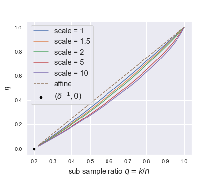
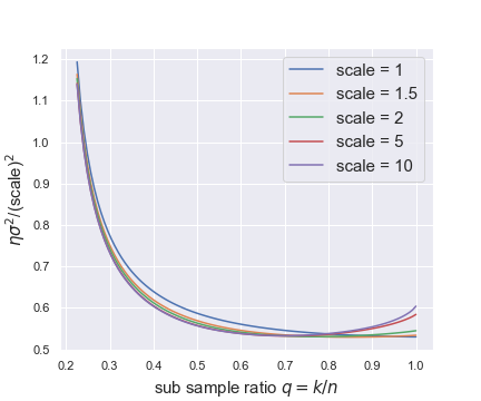
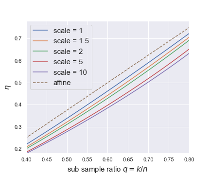
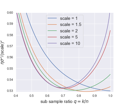
Figure 1: Plot of ${q}\mapsto\eta$ and ${q}\mapsto\sigma^{2}\eta$ obtained by solving (2.4) numerically. Different noise distributions are given by $(\text{scale})\times\text{t-dist (df=2)}$, for scale$\in\{1,{1.5,2,5,}10\}$. The dashed line is the affine line $q\mapsto(q-\delta^{-1})/(1-\delta^{-1})$. The bottom plots zoom in on a specific region of the top plots.

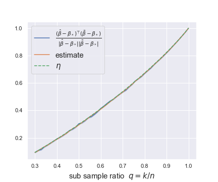
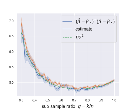
Figure 2: Comparison of simulation results, theoretical curves obtained by solving (2.4) numerically, and estimate constructed by (2.12). Here, the noise distribution is fixed to $3\times\text{t-dist(df=2)}$ and $(n,p)=(5000,1000)$.

Remark 2.4.

The second derivative of the Huber loss $\rho^{\prime\prime}(x)$ is $0$ when $|x|\geq$1, so the condition $\rho^{\prime\prime}>0$ in Assumption 2.1 is not satisfied. However, the numerical simulation in Section 2.5 suggests that (2.11)-(2.12) still hold for the Huber loss and that the condition $\rho^{\prime\prime}>0$ is an artifact of the proof. We expect that the condition $\rho^{\prime\prime}>0$ can be relaxed, at least for a large class of differentiable loss functions including the Huber loss, by adding a vanishing Ridge penalty term to the optimization problem (1.2) as explained in [5].

3 Resampling without replacement in logistic regression

3.1 A review of existing results in logistic regression

Let $\nu>0,q\in(0,1],\delta>1$ be fixed constants. If a single estimator $\hat{\bm{b}}(I)$ is trained with (1.2) on a subset of observations $I\subset[n]$ with $|I|/n=q$ for some constant $q\in(0,1]$ held fixed as $n,p\to+\infty$, the behavior of $\hat{\bm{b}}(I)$ is now well-understood when $(y_{i},\bm{x}_{i})_{i\in[n]}$ are iid with $\bm{x}_{i}\sim N(\bm{0}_{p},\bm{I}_{p})$ normally distributed and the conditional distribution $y_{i}\mid\bm{x}_{i}$ following a logistic model of the form

$$\operatorname{\mathbb{P}}\Bigl{(}y_{i}=1\mid\bm{x}_{i}\Bigr{)}=\frac{1}{1+\exp(-\bm{x}_{i}^{T}\bm{\beta}^{*})}=\frac{1}{1+\exp(-\nu\bm{x}_{i}^{T}\bm{w})}$$ (3.1)

where $\bm{\beta}^{*}$ is a ground truth with $\|\bm{\beta}^{*}\|=\nu$, and $\bm{w}=\bm{\beta}^{*}/\nu$ is the projection of $\bm{\beta}^{*}$ on the unit sphere. In this logistic regression model, the limiting behavior of $\hat{\bm{b}}(I)$ with the logistic loss (1.5) trained using $|I|=(\delta q)p$ samples is characterized as follows: there exists a monotone continuous function $h(\cdot)$ (with explicit expression given in [17]) such that:

$\bullet$ If $\delta q<h(\nu)$ then the logistic MLE (1.2) does not exist with high-probability.

$\bullet$ If $\delta q>h(\nu)$ then there exists a unique [33] solution $(\sigma_{*},a_{*},\gamma_{*})$ to the following the low-dimensional system of equations

$$\tfrac{\sigma^{2}}{\delta q} =\operatorname{\mathbb{E}}[(aU_{i}+\sigma G_{i}-\operatorname{prox}[\gamma\ell_{i}](aU_{i}+\sigma G_{i}))^{2}],$$ (3.2)

$$0 =\operatorname{\mathbb{E}}[(aU_{i}+\sigma G_{i}-\operatorname{prox}[\gamma\ell_{i}](aU_{i}+\sigma G_{i}))],$$ (3.3)

$$1-\tfrac{1}{\delta q} =\sigma^{-1}\operatorname{\mathbb{E}}[G_{i}\operatorname{prox}[\gamma\ell_{i}]^{\prime}(aU_{i}+\sigma G_{i})]$$ (3.4)

where $U_{i}=\bm{x}_{i}^{T}\bm{w}$ and $G_{i}\sim N(0,1)$ is independent of $(\ell_{i},U_{i})$. Above, $\operatorname{prox}[f](x_{0})=\operatorname*{arg\,min}_{x\in\mathbb{R}}(x_{0}-x)^{2}/2+f(x)$ denotes the proximal operator of any convex function $f$ for any $x_{0}\in\mathbb{R}$. In this region $\{\delta q>h(\nu)\}$ where the above system admits a unique solution $(a,\sigma,\gamma)$, the logistic MLE (1.2) exists with high-probability and the following convergence in probability holds,

$$\bm{w}^{T}\hat{\bm{b}}(I) \to^{P}a,$$ (3.5)

$$\qquad\|(\bm{I}_{p}-\bm{w}\bm{w}^{T})\hat{\bm{b}}(I)\|^{2} \to^{P}\sigma^{2},$$ (3.6)

$$\frac{1}{|I|}\sum_{i\in I}\ell_{i}^{\prime}\Bigl{(}\bm{x}_{i}^{T}\hat{\bm{b}}(I)\Bigr{)}^{2} \to^{P}\frac{\sigma^{2}}{\gamma^{2}q\delta}.$$ (3.7)

by [33, 32] for the first two lines and [29, Theorem 2] for the third. Further results are obtained in [17, 33, 37], including asymptotic normality results for individual components $\hat{b}_{j}$ of (1.2). Note that the 3-unknowns system (3.2)-(3.4) is stated in these existing works after integration of the distribution of $y_{i}$. We choose the equivalent formulation (3.2)-(3.4) without integrating the conditional distribution of $y_{i}$ as the form (3.2)-(3.4) is closer to (2.1)-(2.2) from robust regression, and closer and to the quantities naturally appearing in our proofs. In Section 4, this common notation is useful to prove the main results simultaneously for robust linear regression and logistic regression.

While the limit in probability of the correlation $\bar{\bm{b}}^{T}\bm{\beta}^{*}$ can be deduced directly from (3.5), the case of Mean Squared Error (MSE) $\|\bar{\bm{b}}-\bm{\beta}^{*}\|^{2}$ or the correlation $\bar{\bm{b}}^{T}\bm{\beta}^{*}$ is more subtle. To see the crux of the problem, recall $\bm{w}=\bm{\beta}^{*}/\|\bm{\beta}^{*}\|$, define $\bm{P}=(\bm{I}_{p}-\bm{w}\bm{w}^{T})$ for brevity, and consider the decomposition

$$\|\bar{\bm{b}}-\bm{\beta}^{*}\|^{2}=\bigl{(}\bm{w}^{T}(\bar{\bm{b}}-\bm{\beta}^{*})\bigr{)}^{2}+\|\bm{P}\bar{\bm{b}}\|^{2}$$ (3.8)

where the second term is

$$\bigl{(}\bm{w}^{T}(\bar{\bm{b}}-\bm{\beta}^{*})\bigr{)}^{2}+\frac{1}{M^{2}}\sum_{m,m^{\prime}=1}^{M}\hat{\bm{b}}(I_{m})^{T}\bm{P}\hat{\bm{b}}(I_{m^{\prime}}).$$ (3.9)

In order to characterize the limit of the MSE of $\bar{\bm{b}}$, or to characterize the limit of the normalized correlation $\|\bar{\bm{b}}\|^{-1}\bar{\bm{b}}^{T}\bm{\beta}^{*}$, we need to first understand the limit of the inner product

$$\hat{\bm{b}}(I_{m})^{T}\bm{P}\hat{\bm{b}}(I_{m^{\prime}})$$ (3.10)

where $\hat{\bm{b}}(I_{m})$ and $\hat{\bm{b}}(I_{m^{\prime}})$ are trained on two subsamples $I_{m}$ and $I_{m^{\prime}}$ with non-empty intersection. This problem happens to be almost equivalent to the corresponding one in robust regression, and we will prove the following result and Theorem 2.3 simultaneously.

3.2 Main results for logistic regression

Assumption 3.1.

Let $q\in(0,1),\nu>0,\delta>0$ be constants such that $q\delta>h(\nu)$ as $n/p=\delta$ as $n,p\to+\infty$ with $\bm{\beta}^{*}\in\mathbb{R}^{p}$ satisfying $\|\bm{\beta}^{*}\|=\nu$. Assume that $(\bm{x}_{i},y_{i})_{i\in[n]}$ are iid with $y_{i}\in\{0,1\}$ following the logistic model $\operatorname{\mathbb{P}}(y_{i}=1\mid\bm{x}_{i})=1/(1+\exp(-\bm{x}_{i}^{T}\bm{\beta}^{*}))$. Assume that the loss $\ell_{i}$ is the usual binary logistic loss given by (1.5).

In other words, we assume a logistic model with parameters on the side of the phase transition where the MLE exists with high-probability. In this regime, the system (3.2)-(3.4) admits a unique solution $(a,\sigma,\gamma)$ and the convergence in probability (3.5)-(3.7) holds.

Proposition 3.2.

Under Assumption 3.1, the equation

$$\eta=\frac{{q^{2}}\delta\gamma^{2}}{\sigma^{2}}\operatorname{\mathbb{E}}\Bigl{[}\ell_{i}^{\prime}\Bigl{(}\operatorname{prox}[\gamma\ell_{i}](aU_{i}+\sigma G_{i})\Bigr{)}\ell_{i}^{\prime}\Bigl{(}\operatorname{prox}[\gamma\ell_{i}](aU_{i}+\sigma\tilde{G}_{i})\Bigr{)}\Bigr{]}$$ (3.11)

$$\text{ where }\begin{pmatrix}G_{i}\\ \tilde{G}_{i}\end{pmatrix}\sim N\Bigl{(}0_{2},\begin{pmatrix}1&\eta\\ \eta&1\end{pmatrix}\Bigr{)}$$

with unknown $\eta$ admits a unique solution $\eta\in[0,q]$. Above, $U_{i}=\bm{x}_{i}^{T}\bm{\beta}^{*}/\|\bm{\beta}^{*}\|$ and $(G_{i},\tilde{G}_{i})$ are independent of $(y_{i},\ell_{i},U_{i})$.

We omit the proof since it is exactly same as the proof of Proposition 2.2. Similarly to robust regression in Theorem 2.3 the solution $\eta$ to (3.11) characterizes the limit in probability of the correlation (3.10), the estimator (2.12) is still valid for estimating $\eta\sigma^{2}$, and finally we can characterize the joint distribution of two predicted values $\bm{x}_{i}^{T}\hat{\bm{b}}(I_{m})$ and $\bm{x}_{i}^{T}\hat{\bm{b}}(I_{m})$ for an observation $i\in I_{m}\cap I_{m^{\prime}}$ appearing in both datasets.

Theorem 3.3.

Let Assumption 3.1 be fulfilled and let $\bm{P}=\bm{I}_{p}-\bm{\beta}^{*}\frac{1}{\|\bm{\beta}^{*}\|^{2}}\bm{\beta}^{*}{}^{T}$. Let $I,\tilde{I}$ be independent and uniformly distributed over all subsets of $[n]$ of size $qn$. Then

$$\hat{\bm{b}}(I)\bm{P}\hat{\bm{b}}(\tilde{I})\to^{P}\sigma^{2}\eta,\qquad\frac{\hat{\bm{b}}(I)^{T}\bm{P}\hat{\bm{b}}(\tilde{I})}{\|\bm{P}\hat{\bm{b}}(I)\|_{2}\|\bm{P}\hat{\bm{b}}(\tilde{I})\|_{2}}\to^{P}\eta$$ (3.12)

where $\eta\in[0,q]$ is the unique solution to (3.11). Furthermore, $\eta$ and $\eta\sigma^{2}$ can be consistently estimated in the sense that (2.12) holds. Finally, for any $i\in I\cap\tilde{I}$, there exists $(G_{i},\tilde{G}_{i})$ as in (2.5), independent of $(y_{i},U_{i})$ such that

$$\max_{i\in I\cap\tilde{I}}\operatorname{\mathbb{E}}\Bigl{[}1\wedge\Big{\|}\begin{pmatrix}\bm{x}_{i}^{T}\hat{\bm{b}}(I)\\ \bm{x}_{i}^{T}\hat{\bm{b}}(\tilde{I})\end{pmatrix}-\begin{pmatrix}\operatorname{prox}[\gamma\ell_{i}](aU_{i}+\sigma G_{i})\\ \operatorname{prox}[\gamma\ell_{i}](aU_{i}+\sigma\tilde{G}_{i})\\ \end{pmatrix}\Big{\|}_{2}\mid(I,\tilde{I})\Bigr{]}\to^{P}0.$$ (3.13)

3.3 Numerical simulations in logistic regression

Similarly to Section 2.5, we check the accuracy of Theorem 3.3 with numerical simulations. Here, $(n,p)$ is fixed to $(5000,500)$ so that $\delta=n/p=10$. For each signal strength $\|\bm{\beta}_{*}\|\in\{1,2\}$, we compute the correlation

$$\hat{\bm{b}}(I)^{T}\bm{P}\hat{\bm{b}}(\tilde{I})/\bigl{(}\|\bm{P}\hat{\bm{b}}(I)\|_{2}\|\bm{P}\hat{\bm{b}}(\tilde{I})\|_{2}\bigr{)}$$

and the inner product $\hat{\bm{b}}(I)^{T}\bm{P}\hat{\bm{b}}(\tilde{I})$ as we change the sub-sampling ratio $q=k/n\in[0.4,1]$ and the estimate constructed by (2.12). We perform $100$ repetitions. The theoretical limits $(\eta,\sigma^{2}\eta)$ are obtained by solving (3.11) numerically. Figure 3 shows that the theoretical curves ($q\mapsto\eta$ and $q\mapsto\sigma^{2}\eta$) match with the correlation and the inner product. The estimator (2.12) is accurate for medium to large subsample ratio $q$, but appears slightly biased upwards for small values of $q$. The source of this slight upward bias is unclear, although possibly due to the finite-sample nature of the simulations $(p=500)$.

In all simulations for logistic regression that we have performed, the curve $q\mapsto\eta$ is affine, as in the left plot in Figure 3. The reason for this is unclear to us at this point and this appears to be specific logistic regression; for instance the curve $q\mapsto\eta$ in Figure 1 for robust regression are clearly non-affine.

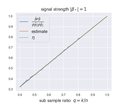
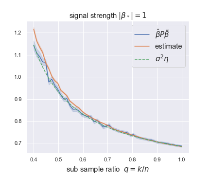
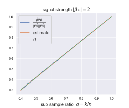
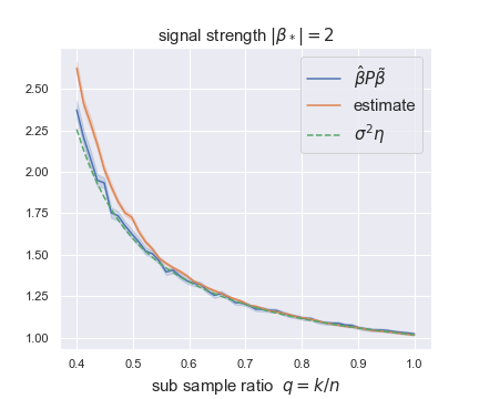
Figure 3: Comparison of simulation results, theoretical curves obtained by solving (3.11) numerically, and estimate constructed by (2.12), with $(n,p)$ fixed to $(2500,250)$.

4 Proof of the main results

We prove here Theorems 3.3 and 2.3 simultaneously using the following notation:

• In Robust regression (Theorem 2.3), set $a=0$, let $(\sigma,\gamma)$ be the unique solution to (2.1)-(2.2), let $\bm{\beta}^{*}=0$ (without loss of generality thanks to translation invariance), and let $\bm{P}=\bm{I}_{p}$. Furthermore, let $U_{i}=0$.

• In logistic regression (Theorem 3.3), let $(a,\sigma,\gamma)$ be the unique solution to (3.2)-(3.4), let $\bm{P}=\bm{I}_{p}-\bm{w}\bm{w}^{\top}$ for $\bm{w}=\beta^{*}/\|\bm{\beta}^{*}\|$, and let $U_{i}=\bm{x}_{i}^{T}\bm{w}$. Here, $\bm{X}\bm{P}$ is independent of $(y_{i},\ell_{i},U_{i})_{i\in[n]}$.

Thanks to $\|\bm{X}/\sqrt{n}\|_{op}\to^{P}1+\delta^{-1/2}$ and (2.10) or (3.6)-(3.5), we have $\|\bm{X}\hat{\bm{b}}(I)\|/\sqrt{I}\leq K$ for $K=2q^{-1/2}(1+\delta^{-1/2})(a^{2}+\sigma^{2})^{1/2}$ with probability approaching one. Thus $\operatorname{\mathbb{P}}(\hat{\bm{b}}(I)=\bm{\hat{\beta}}(I))\to 1$ for $\bm{\hat{\beta}}(I)$ in (5.8), so we may argue with $\bm{\hat{\beta}}=\bm{\hat{\beta}}(I)$. Similarly for $\tilde{I}$ we have $\operatorname{\mathbb{P}}(\hat{\bm{b}}(I)=\bm{\hat{\beta}}(I))\to 1$ for $\bm{\hat{\beta}}(\tilde{I})$ in (5.8), and we may argue with $\bm{\tilde{\beta}}=\bm{\hat{\beta}}(\tilde{I})$. Let also $\bm{\psi},\bm{\tilde{\psi}}$ be defined in Lemma 5.4 (in particular, we have $\psi_{i}=0$ of $i\notin I$ and $\psi_{i}=-\ell_{i}(\bm{x}_{i}^{T}\hat{\bm{b}}(I))$ in the high-probability event $\hat{\bm{b}}(I)=\bm{\hat{\beta}}$, and similarly for $\bm{\tilde{\psi}},\hat{\bm{b}}(\tilde{I}),\bm{\tilde{\beta}}$.)

By (5.11) and (5.16) from the auxiliary lemmas, we have

$$p\hat{\bm{\beta}}^{\top}\bm{P}\tilde{\bm{\beta}}=\gamma^{2}\bm{\psi}^{\top}\tilde{\bm{\psi}}+O_{P}(\sqrt{n})$$

where $\bm{\psi}^{\top}\tilde{\bm{\psi}}=\sum_{i\in I\cap\tilde{I}}\psi_{i}\tilde{\psi}_{i}$. With $n/p=\delta$ and $|I\cap\tilde{I}|=nq^{2}+O_{P}(n^{1/2})$ thanks to the explicit formulae for the expectation and variance of the hyper-geometric distribution, we have

$$\tilde{\bm{\beta}}^{\top}\bm{P}\hat{\bm{\beta}}=\delta q^{2}\gamma^{2}\bm{\psi}^{T}\bm{\tilde{\psi}}/|I\cap\tilde{I}|+O_{P}(n^{-1/2}).$$ (4.1)

By the Cauchy–Schwarz inequality and the concentration of sampling without replacement (Lemma 5.12) (or see Lemma 5.8 for details), the absolute value of $\bm{\psi}^{T}\bm{\tilde{\psi}}/|I\cap\tilde{I}|=\frac{1}{|I\cap\tilde{I}|}\sum_{i\in I\cap\tilde{I}}\psi_{i}\tilde{\psi}_{i}$ is smaller than

$$\Bigl{(}\frac{1}{|I\cap\tilde{I}|}\sum_{i\in I\cap\tilde{I}}\tilde{\psi}_{i}^{2}\Bigr{)}^{1/2}\Bigl{(}\frac{1}{|I\cap\tilde{I}|}\sum_{i\in I\cap\tilde{I}}\psi_{i}^{2}\Bigr{)}^{1/2}\\ \leq\Bigl{(}\frac{1}{|\tilde{I}|}\sum_{i\in\tilde{I}}\tilde{\psi}_{i}^{2}\Bigr{)}^{1/2}\Bigl{(}\frac{1}{|\tilde{I}|}\sum_{i\in I}\psi_{i}^{2}\Bigr{)}^{1/2}+o_{P}(1)=\frac{\sigma^{2}}{q\delta\gamma^{2}}+o_{P}(1)$$

thanks to (2.10) (in robust regression) or (3.7) (in logistic regression) for the last equality. Combined with (4.1), we have proved $|\tilde{\bm{\beta}}^{\top}\bm{P}\hat{\bm{\beta}}|\leq\delta q^{2}\gamma^{2}\frac{\sigma^{2}}{q\delta\gamma^{2}}+o_{P}(1)=q\sigma^{2}+o_{P}(1).$ Let $\bar{\operatorname{\mathbb{E}}}$ be the conditional expectation given $({I,\tilde{I}},\bm{X}\bm{\beta}^{*},\bm{y})$ (In robust regression, $\bm{\beta}^{*}=0$ so $\bar{\operatorname{\mathbb{E}}}$ is the conditional expectation given $\{{I,\tilde{I}},(\varepsilon_{i})_{i\in[n]}\}$). Thanks to the the Gaussian Poincaré inequality in Lemma 5.9,

$$\bar{\eta}\coloneqq\sigma^{-2}\bar{\operatorname{\mathbb{E}}}[\tilde{\bm{\beta}}^{\top}\bm{P}\hat{\bm{\beta}}]\quad\text{ satisfies }\quad\begin{cases}\bar{\eta}=\tilde{\bm{\beta}}^{\top}\bm{P}\hat{\bm{\beta}}/\sigma^{2}+O_{P}(n^{-1/2}),\\ |\bar{\eta}|\leq q+o_{P}(1).\end{cases}$$ (4.2)

Similarly, by Lemma 5.9 we have $\bar{\operatorname{\mathbb{E}}}[\bm{\psi}^{T}\bm{\tilde{\psi}}]/{|I\cap\tilde{I}|}=\bm{\psi}^{T}\bm{\tilde{\psi}}/{|I\cap\tilde{I}|}+O_{P}(n^{-1/2})$. Combining the previous displays gives

$$\bar{\eta}=\frac{\delta q^{2}\gamma^{2}}{\sigma^{2}}\frac{1}{|I\cap\tilde{I}|}\bar{\operatorname{\mathbb{E}}}\Bigl{[}\sum_{i\in I\cap\tilde{I}}\psi_{i}\tilde{\psi}_{i}\Bigr{]}+o_{P}(1).$$ (4.3)

For an overlapping observation $i\in I\cap\tilde{I}$, using the derivative formula in Lemma 5.4 and the moment inequality in Proposition 5.1 conditionally on $(I,\tilde{I},\bm{X}\bm{\beta}^{*},\bm{y})$ and $(\bm{x}_{l})_{l\neq i}$, applied to the standard normal $\bm{P}\bm{x}_{i}+\bm{w}Z$ (for $Z\sim N(0,1)$ independent of everything else) and $\bm{W}=[\bm{P}\hat{\bm{\beta}}|\bm{P}\tilde{\bm{\beta}}]\in\mathbb{R}^{p\times 2}$, we find for the indicator function $\mathbb{I}\{i\in I\cap\tilde{I}\}$ that $\mathbb{I}\{i\in I\cap\tilde{I}\}\operatorname{\mathbb{E}}[\text{LHS}_{i}\mid I,\tilde{I}]\leq C\operatorname{\mathbb{E}}[\sum_{j=1}^{p}\|\frac{\partial\hat{\bm{\beta}}}{\partial x_{ij}}\|^{2}+\|\frac{\partial\tilde{\bm{\beta}}}{\partial x_{ij}}\|^{2}]$ where

$$\text{LHS}_{i}\eqqcolon\Bigl{\|}\begin{pmatrix}\bm{x}_{i}^{\top}\bm{P}\hat{\bm{\beta}}-\operatorname{tr}[\bm{P}\bm{A}]\psi_{i}-(\hat{\bm{\beta}}^{\top}\bm{P}\bm{A}\bm{X}^{\top}\bm{D})\bm{e}_{i}\\ \bm{x}_{i}^{\top}\bm{P}\tilde{\bm{\beta}}-\operatorname{tr}[\bm{P}\tilde{\bm{A}}]\tilde{\psi}_{i}-(\tilde{\bm{\beta}}^{\top}\bm{P}\tilde{\bm{A}}\bm{X}^{\top}\tilde{\bm{D}})\bm{e}_{i}\end{pmatrix}-(\bm{W}^{\top}\bm{W})^{1/2}\bm{g}_{i}\Bigr{\|}^{2}$$

for all $i\in I\cap\tilde{I}$, where $\bm{g}_{i}\sim N(\bm{0}_{2},\bm{I}_{2})$. After summing over $i\in I\cap\tilde{I}$ and using (5.13), we get $\sum_{i\in I\cap\tilde{I}}\operatorname{\mathbb{E}}[\text{LHS}_{i}\mid I,\tilde{I}]\leq C$ and

$$\frac{1}{n}\sum_{i\in I\cap\tilde{I}}\operatorname{\mathbb{E}}\Bigl{[}\text{LHS}_{i}\mid I,\tilde{I}\Bigr{]}\leq\frac{C^{\prime}}{n},\qquad\frac{1}{n}\sum_{i\in I\cap\tilde{I}}\text{LHS}_{i}=O_{{p}}\Bigl{(}\frac{1}{n}\Bigr{)}$$

for some deterministic constants $C,C^{\prime}$ independent of $n,p$.

Using (3.6) in logistic regression or (2.10) in robust regression, we know $\|\bm{P}\hat{\bm{\beta}}\|^{2}\to^{P}\sigma^{2}$ and similarly $\|\bm{P}\tilde{\bm{\beta}}\|^{2}\to^{P}\sigma^{2}$, as well as $\operatorname{tr}[\bm{P}\bm{A}]\to^{P}\gamma$, and $\operatorname{tr}[\bm{P}\tilde{\bm{A}}]\to^{P}\gamma$ by (5.16). Using the Lipschitz inequality for the matrix square root $\|\sqrt{\bm{M}}-\sqrt{\bm{N}}\|_{op}\leq\|(\sqrt{\bm{M}}+\sqrt{\bm{N}})^{-1}\|_{op}\|\bm{M}-\bm{N}\|_{op}$ for positive definite matrices $\bm{N},\bm{M}$ [35] [11, Problem X.5.5] which follows from $\bm{x}^{T}(\sqrt{\bm{M}}+\sqrt{\bm{N}})\bm{x}\lambda=\bm{x}^{T}(\bm{M}-\bm{N})\bm{x}$ for any unit eigenvector $\bm{x}$ of $\sqrt{\bm{M}}-\sqrt{\bm{N}}$ with eigenvalue $\lambda$, here we get

$$\Big{\|}\begin{pmatrix}1&\bar{\eta}\\ \bar{\eta}&1\\ \end{pmatrix}^{-1}\Big{\|}_{op}=\frac{1}{1-\bar{\eta}}\leq\frac{2}{1-q}\text{ and }\Big{\|}\sigma\begin{pmatrix}1&\bar{\eta}\\ \bar{\eta}&1\\ \end{pmatrix}^{1/2}-(\bm{W}^{\top}\bm{W})^{1/2}\Big{\|}_{op}=o_{P}(1)$$ (4.4)

on the event $|\bar{\eta}|\leq(1+q)/2<1$ which has probability approaching one thanks to (4.2). Using the moment bounds (5.10) to bound from above $\sum_{i=1}^{n}((\hat{\bm{\beta}}^{\top}\bm{P}\bm{A}\bm{X}^{\top}\bm{D})\bm{e}_{i})^{2}=\|\bm{D}\bm{X}\bm{A}\bm{P}\bm{\hat{\beta}}\|^{2}$, we find

$$\frac{1}{n}\sum_{i\in I\cap\tilde{I}}\|\begin{pmatrix}\bm{x}_{i}^{\top}\bm{P}\hat{\bm{\beta}}-\gamma\psi_{i}\\ \bm{x}_{i}^{\top}\bm{P}\tilde{\bm{\beta}}-\gamma\tilde{\psi}_{i}\end{pmatrix}-\sigma\begin{pmatrix}1&\bar{\eta}\\ \bar{\eta}&1\\ \end{pmatrix}^{1/2}\bm{g}_{i}\|^{2}=o_{P}(1)+o_{P}(1)\frac{1}{n}\sum_{i=1}^{n}\bigl{(}\|\bm{g}_{i}\|^{2}+\psi_{i}^{2}+\tilde{\psi}_{i}^{2}\bigr{)},$$

and thanks to $\frac{1}{n}\sum_{i=1}^{n}(\|\bm{g}_{i}\|^{2}+\psi_{i}^{2}+\tilde{\psi}_{i}^{2})=O_{P}(1)$, the previous display converges to 0 in probability. Since $\bm{x}_{i}^{T}\bm{P}\bm{\hat{\beta}}=\bm{x}_{i}^{T}\bm{\hat{\beta}}-U_{i}\bm{w}^{T}\bm{\hat{\beta}}$ for $U_{i}=\bm{x}_{i}^{T}\bm{w}=^{d}N(0,1)$ and given $\hat{\bm{\beta}}^{\top}\bm{w}\to^{P}a$ by (3.5), together with $\frac{1}{n}\sum_{i=1}U_{i}^{2}=O_{P}(1)$ since $\sum_{i=1}U_{i}^{2}\sim\chi^{2}_{n}$ we find

$$\frac{1}{n}\sum_{i\in I\cap\tilde{I}}\|\begin{pmatrix}\bm{x}_{i}^{\top}\hat{\bm{\beta}}-aU_{i}-\gamma\psi_{i}-\sigma G_{i}\\ \bm{x}_{i}^{\top}\tilde{\bm{\beta}}-aU_{i}-\gamma\tilde{\psi}_{i}-\sigma\tilde{G}_{i}\end{pmatrix}\|^{2}=o_{P}(1)~{}~{}\text{ where}~{}~{}\begin{pmatrix}G_{i}\\ \tilde{G}_{i}\end{pmatrix}=\begin{pmatrix}1&\bar{\eta}\\ \bar{\eta}&1\\ \end{pmatrix}^{1/2}\bm{g}_{i}.$$

With probability approaching one, the second term in (5.8) is 0 for the large enough $K$ that we took at the beginning, and in this event the modified M-estimator $\hat{\bm{\beta}}$ equals to the original M-estimator $\hat{\bm{b}}(I)$ so that $\psi_{i}=-\ell_{i}(\bm{x}_{i}^{\top}\hat{\bm{b}})$ (cf. Lemma 5.3), and similarly for $\tilde{\bm{\psi}}$. We have established

$$\frac{1}{n}\sum_{i\in I\cap\tilde{I}}\|\underbrace{\bm{x}_{i}^{\top}\hat{\bm{b}}+\gamma\ell_{i}^{\prime}(\bm{x}_{i}^{\top}\hat{\bm{b}})-aU_{i}-\sigma G_{i}}_{-\text{Rem}_{i}}\|^{2}=o_{P}(1).$$

Define $\text{Rem}_{i}$ by $\bm{x}_{i}^{\top}\hat{\bm{b}}+\gamma\ell_{i}^{\prime}(\bm{x}_{i}^{\top}\hat{\bm{b}})=aU_{i}+\sigma G_{i}+\text{Rem}_{i}$ so that $\bm{x}_{i}^{\top}\hat{\bm{b}}=\operatorname{prox}[\gamma\ell_{i}](aU_{i}+\sigma G_{i}+\text{Rem}_{i})$ by definition of the proximal operator. Now set $\hat{p}_{i}=\operatorname{prox}[\gamma\ell_{i}](aU_{i}+\sigma G_{i})$. Because $\operatorname{prox}[\gamma\ell_{i}](\cdot)$ is 1-Lipschitz,

$$\Bigl{(}\sum_{i\in I\cap\tilde{I}}\|\hat{p}_{i}-\bm{x}_{i}^{\top}\hat{\bm{b}}\|^{2}\Bigr{)}^{1/2}\leq\Bigl{(}\sum_{i\in I\cap\tilde{I}}\|\text{Rem}_{i}\|^{2}\Bigr{)}^{1/2}=o_{P}({\sqrt{n}}).$$

Similarly, a proximal approximation holds for $\bm{x}_{i}^{\top}\tilde{\bm{\beta}}$ using $(U_{i},\tilde{G}_{i})$ instead. We have to be a little careful here because $\bar{\eta}$ is independent of the $(G_{i},\tilde{G}_{i})$ but not of the $(U_{i},y_{i})$. Using that $|\ell_{i}^{\prime}|\leq 1$, and that $\bar{E}[|A-B|]=o_{P}(1)$ if $A,B$ are bounded random variables such that $|A-B|=o_{P}(1)$, (4.3) gives

$$\bar{\eta} =\frac{\delta q^{2}\gamma^{2}}{\sigma^{2}}\sum_{i\in I\cap\tilde{I}}\bar{\operatorname{\mathbb{E}}}\Bigl{[}\frac{\ell_{i}^{\prime}(\operatorname{prox}[\gamma\ell_{i}](aU_{i}+\sigma G_{i}))\ell_{i}^{\prime}(\operatorname{prox}[\gamma\ell_{i}](aU_{i}+\sigma\tilde{G}_{i}))}{|I\cap\tilde{I}|}\Bigr{]}+o_{P}(1)$$

where inside the conditional expectation $\bar{\operatorname{\mathbb{E}}}[\cdot]$, $(\bar{\eta},U_{i},\ell_{i})$ are fixed are integration is performed with respect to the distribution of $(G_{i},\tilde{G}_{i})$, so that $\bar{\eta}=\frac{\delta q^{2}\gamma^{2}}{\sigma^{2}}\varphi(\bar{\eta})+o_{P}(1)$ where

$$\varphi(t) =\frac{1}{|I\cap\tilde{I}|}\sum_{i\in I\cap\tilde{I}}\bar{\operatorname{\mathbb{E}}}\Bigl{[}\ell_{i}^{\prime}\Bigl{(}\operatorname{prox}[\gamma\ell_{i}](aU_{i}+\sigma G_{i}^{t})\Bigr{)}\ell_{i}^{\prime}\Bigl{(}\operatorname{prox}[\gamma\ell_{i}](aU_{i}+\sigma\tilde{G}_{i}^{t})\Bigr{)}\Bigr{]}$$

$$=\frac{1}{|I\cap\tilde{I}|}\sum_{i\in I\cap\tilde{I}}\iint\ell_{i}^{\prime}\Bigl{(}\operatorname{prox}[\gamma\ell_{i}](aU_{i}+\sigma g)\Bigr{)}\ell_{i}^{\prime}\Bigl{(}\operatorname{prox}[\gamma\ell_{i}](aU_{i}+\sigma\tilde{g})\Bigr{)}\phi_{t}(g,\tilde{g})\mathrm{d}g\mathrm{d}\tilde{g}$$

where $\phi_{t}$ is the joint density of two jointly normal $(G^{t},\tilde{G}^{t})$ with $\operatorname{\mathbb{E}}[(G^{t})^{2}]=\operatorname{\mathbb{E}}[(\tilde{G}^{t})^{2}]=1$ and $\operatorname{\mathbb{E}}[G^{t}\tilde{G}^{t}]=t$, and in the first line $(G_{i}^{t},\tilde{G}_{i}^{t})\sim\phi_{t}$ is independent of $(\bar{\eta},U_{i},y_{i},\ell_{i})_{i\in[n]}$. Because of the law of large numbers for the deterministic solution $\eta$ of (2.4) (with $a=0$ in robust regression) or (3.11) (in logistic regression), we have $\eta=\frac{\delta^{2}q^{2}\gamma^{2}}{\sigma^{2}}\varphi(\eta){+o_{P}(1)}$. Taking the difference between the previous display and this fixed-point equation satisfied by $\eta$, using the mean-value theorem,

$$\bar{\eta}-\eta=\frac{\delta q^{2}\gamma^{2}}{\sigma^{2}}\Bigl{(}\varphi(\bar{\eta})-\varphi(\eta)\Bigr{)}+o_{P}(1)=\frac{\delta q^{2}\gamma^{2}}{\sigma^{2}}\Bigl{(}\bar{\eta}-\eta\Bigr{)}\varphi^{\prime}(t)+o_{P}(1)$$

for some $t\in[\bar{\eta},\eta]$. By calculation similar to (2.8)-(2.9) thanks to Lemma 5.2, if $(G_{i}^{t},\tilde{G}_{i}^{t})$ has density $\phi_{t}$,

$$\varphi^{\prime}(t) =\frac{1}{|I\cap\tilde{I}|}\frac{\sigma^{2}}{\gamma^{2}}\sum_{i\in I\cap\tilde{I}}\bar{\operatorname{\mathbb{E}}}\Bigl{[}\frac{\gamma\ell_{i}^{\prime\prime}(\operatorname{prox}[\gamma\ell_{i}](aU_{i}+\sigma G_{i}^{t}))}{1+\gamma\ell_{i}^{\prime\prime}(\operatorname{prox}[\gamma\ell_{i}](aU_{i}+\sigma G_{i}^{t}))}\frac{\gamma\ell_{i}^{\prime\prime}(\operatorname{prox}[\gamma\ell_{i}](aU_{i}+\sigma\tilde{G}_{i}^{t}))}{1+\gamma\ell_{i}^{\prime\prime}(\operatorname{prox}[\gamma\ell_{i}](aU_{i}+\sigma\tilde{G}_{i}^{t}))}\Bigr{]}$$

$$\leq\frac{1}{|I\cap\tilde{I}|}\frac{\sigma^{2}}{\gamma^{2}}\sum_{i\in I\cap\tilde{I}}\bar{\operatorname{\mathbb{E}}}\Bigl{[}\frac{\gamma\ell_{i}^{\prime\prime}(\operatorname{prox}[\gamma\ell_{i}](aU_{i}+\sigma G_{i}^{t}))}{1+\gamma\ell_{i}^{\prime\prime}(\operatorname{prox}[\gamma\ell_{i}](aU_{i}+\sigma G_{i}^{t}))}\Bigr{]}$$

$$=\frac{1}{|I\cap\tilde{I}|}\frac{\sigma^{2}}{\gamma^{2}}\sum_{i\in I\cap\tilde{I}}\int\Bigl{[}\frac{\gamma\ell_{i}^{\prime\prime}(\operatorname{prox}[\gamma\ell_{i}](aU_{i}+\sigma g))}{1+\gamma\ell_{i}^{\prime\prime}(\operatorname{prox}[\gamma\ell_{i}](aU_{i}+\sigma g))}\Bigr{]}\frac{e^{-g^{2}/2}}{\sqrt{2\pi}}\mathrm{d}g\quad\text{since }G_{i}^{t}\sim N(0,1)$$

$$=\frac{\sigma^{2}}{\gamma^{2}q\delta}+o_{P}(1),$$

where we have used the law of large numbers and the nonlinear system with equation (2.2) in robust regression and equation (3.4) in logistic regression. Combining the above displays, we are left with

$$|\bar{\eta}-\eta|=|\bar{\eta}-\eta|\frac{\delta q^{2}\gamma^{2}}{\sigma^{2}}|\varphi^{\prime}(t)|+o_{P}(1)\leq|\bar{\eta}-\eta|\frac{\delta q^{2}\gamma^{2}}{\sigma^{2}}\frac{\sigma^{2}}{\gamma^{2}q\delta}+o_{P}(1)=q|\bar{\eta}-\eta|+o_{P}(1)$$

and $\bar{\eta}-\eta=o_{P}(1)$ thanks to $q\in(0,1)$. Since $\bar{\eta}=\hat{\bm{\beta}}^{\top}\bm{P}\tilde{\bm{\beta}}/\sigma^{2}+o_{P}(1)$ by (4.2), the proof of (2.11) and (3.12) is complete. Next, (2.12) follows from (5.11) and (5.16).

Finally for (2.13) and (3.13), by symmetry $\operatorname{\mathbb{E}}[\text{LHS}_{i}\mid I,\tilde{I}]$ is the same for all $i\in I\cap\tilde{I}$. In particular, the maximum of the conditional expectation is the same as the average over $I\cap\tilde{I}$, so that $\sum_{i\in I\cap\tilde{I}}\operatorname{\mathbb{E}}[\text{LHS}_{i}\mid I,\tilde{I}]\leq C$ proved above gives $\max_{i\in I\cap\tilde{I}}\operatorname{\mathbb{E}}[\text{LHS}_{i}\mid I,\tilde{I}]=O_{P}(1/n)$ since $I\cap\tilde{I}$ has cardinality of order $n$. Finally, we have

$$\bm{W}^{\top}\bm{W}\to^{P}\sigma^{2}\begin{pmatrix}1&\eta\\ \eta&1\end{pmatrix},\qquad\Bigl{(}\bm{W}^{\top}\bm{W}\Bigr{)}^{1/2}\to^{P}\sigma\begin{pmatrix}1&\eta\\ \eta&1\end{pmatrix}^{1/2},$$ (4.5)

by continuity of the matrix square root and the continuous mapping theorem (or, alternatively, by reusing the argument in (4.4)). Using again $\operatorname{tr}[\bm{P}\bm{A}]\to^{P}\gamma$, $\bm{\hat{\beta}}^{T}\bm{w}\to^{P}a$, $(\hat{\bm{\beta}}^{\top}\bm{P}\bm{A}\bm{X}^{\top}\bm{D})\bm{e}_{i}\to^{P}0$, and similarly for $\bm{\tilde{\beta}}$, combined with (4.5), we obtain (2.13) and (3.13).

5 Auxiliary lemmas

5.1 Approximate multivariate normality

Proposition 5.1.

Let $\bm{z}\sim N(\bm{0}_{p},\bm{I}_{p})$ and let $\bm{W}:\mathbb{R}^{n}\to\mathbb{R}^{p\times M}$ be a locally Lipschitz function with $M\leq p$. Then there exists $\bm{g}\sim N(\bm{0}_{M},\bm{I}_{M})$ such that

$$\operatorname{\mathbb{E}}\Bigl{[}\bigl{\|}\bm{W}(\bm{z})^{\top}\bm{z}-\sum_{j=1}^{p}\frac{\partial\bm{W}(\bm{z})^{\top}\bm{e}_{j}}{\partial z_{j}}-\Bigl{\{}\bm{W}(\bm{z})^{\top}\bm{W}(\bm{z})\Bigr{\}}^{1/2}\bm{g}\bigr{\|}^{2}\Bigr{]}\leq\C\sum_{j=1}^{p}\operatorname{\mathbb{E}}\Bigl{[}\bigl{\|}\frac{\partial\bm{W}(z)}{\partial z_{j}}\bigr{\|}_{F}^{2}\Bigr{]},$$

where $\{\cdot\}^{1/2}$ is the square root of the positive semi-definite matrix.

This moment inequality is a matrix-generalization of [7, Proposition 13] and [9, Theorem 2.2]. It is particularly useful to show that

$$\bm{W}(\bm{z})^{\top}\bm{z}-\sum_{j=1}^{p}\frac{\partial\bm{W}(\bm{z})^{\top}\bm{e}_{j}}{\partial z_{j}}$$

is approximately multivariate normal with covariance approximated by $\bm{W}(\bm{z})^{\top}\bm{W}(\bm{z})$.

Proof.

Let $\tilde{\bm{z}}$ be an independent copy of $\bm{z}$ and let $\tilde{\bm{W}}=\bm{W}(\tilde{\bm{z}})$. Noting $M\leq p$, we denote the SVD of $\tilde{\bm{W}}\in\mathbb{R}^{p\times M}$ by $\tilde{\bm{W}}=\sum_{m=1}^{M}s_{m}\bm{u}_{m}\bm{v}_{m}^{\top}$ where $s_{1}\geq s_{2}\geq...\geq s_{M}\geq 0$ are the singular values. Here, we allow some $s_{m}$ to be $0$ to have $M$ terms by adding extra terms if necessary, so that $(\bm{v}_{1},...,\bm{v}_{M})$ is an orthonormal basis in $\mathbb{R}^{M}$. Now we define

$$\tilde{\bm{Q}}=\sum_{m=1}^{M}\bm{v}_{m}\bm{u}_{m}^{\top}\in\mathbb{R}^{M\times p}$$

so that $\tilde{\bm{W}}=\tilde{\bm{Q}}^{\top}(\tilde{\bm{W}}^{\top}\tilde{\bm{W}})^{1/2}$ thanks to $(\tilde{\bm{W}}^{\top}\tilde{\bm{W}})^{1/2}=\sum_{m=1}^{M}s_{m}\bm{v}_{m}\bm{v}_{m}^{\top}$. Define $\bm{g}=\tilde{\bm{Q}}\bm{z}$ and note that$\bm{g}\sim N(\bm{0}_{M},\bm{I}_{M})$ since $\tilde{\bm{W}}=\bm{W}(\tilde{\bm{z}})$ is independent of $\bm{z}$. With $\bm{W}=\bm{W}(\bm{z})$ (omitting the dependence in $\bm{z}$), using $\bm{g}=\tilde{\bm{Q}}\bm{z}$ and $\tilde{\bm{W}}=\tilde{\bm{Q}}^{\top}(\tilde{\bm{W}}^{\top}\tilde{\bm{W}})^{1/2}$, we have

$$\tilde{\bm{W}}^{\top}\bm{z}-(\bm{W}^{\top}\bm{W})^{1/2}\bm{g}=\bigl{[}(\tilde{\bm{W}}^{\top}\tilde{\bm{W}})^{1/2}-(\bm{W}^{\top}\bm{W})^{1/2}\bigr{]}\bm{g}.$$

Applying the Second order Stein formula [8] (see also 5.1.13 in [12]) to $\bm{U}(\bm{z})=\bm{W}(z)^{\top}-\{\bm{W}(z)^{\top}\bm{W}(\bm{z})\}^{1/2}\tilde{\bm{Q}}\in\mathbb{R}^{M\times p}$ conditionally on $(\tilde{\bm{z}},\tilde{\bm{Q}})$, we find

$$\operatorname{\mathbb{E}}\Bigl{[}\|\bm{W}^{\top}\bm{z}-\sum_{j=1}^{p}\frac{\partial(\bm{W}^{\top}-\{\bm{W}^{\top}\bm{W}\}^{1/2}\tilde{\bm{Q}})\bm{e}_{j}}{\partial z_{j}}-\{\bm{W}^{\top}\bm{W}\}^{1/2}\bm{g}\|^{2}\Bigr{]}$$

$$=\operatorname{\mathbb{E}}\bigl{[}\|\bm{U}\bm{z}-\sum_{j=1}^{p}\frac{\partial\bm{U}\bm{e}_{j}}{\partial z_{j}}\|^{2}\bigr{]} \bm{g}=\tilde{\bm{Q}}\bm{z}$$

$$\leq\operatorname{\mathbb{E}}\Bigl{[}\|\bm{U}(\bm{z})\|_{F}^{2}+\sum_{j=1}^{p}\|\frac{\partial\bm{U}(\bm{z})}{\partial z_{j}}\|_{F}^{2}\Bigr{]}.$$ (5.1)

Since $\tilde{\bm{W}}^{\top}=(\tilde{\bm{W}}^{\top}\tilde{\bm{W}})^{1/2}\tilde{\bm{Q}}$, by the triangle inequality,

$$\|\bm{U}\|_{F} =\|\bm{W}^{\top}-\{\bm{W}^{\top}\bm{W}\}^{1/2}\tilde{\bm{Q}}\|_{F}$$

$$\leq\|\bm{W}-\tilde{\bm{W}}\|_{F}^{2}+\|\tilde{\bm{W}}^{\top}-(\bm{W}^{\top}\bm{W})^{1/2}\tilde{\bm{Q}}\|_{F}^{2}$$ (5.2)

$$=\|\bm{W}-\tilde{\bm{W}}\|_{F}+\|[(\tilde{\bm{W}}^{\top}\tilde{\bm{W}})-(\bm{W}^{\top}\bm{W})^{1/2}]\tilde{\bm{Q}}\|_{F}$$

$$\leq\|\bm{W}-\tilde{\bm{W}}\|_{F}+\sqrt{2}\|\bm{W}-\tilde{\bm{W}}\|_{F}$$ (5.3)

thanks to $\|\tilde{\bm{Q}}\|_{op}\leq 1$ and using, for the last line, inequality

$$\|(\tilde{\bm{W}}^{\top}\tilde{\bm{W}})^{1/2}-(\bm{W}^{\top}\bm{W})^{1/2}\|_{F}\leq\sqrt{2}\|\bm{W}-\tilde{\bm{W}}\|_{F}$$ (5.4)

from [1, 19]. Now for the second term in (5.1),

$$\sum_{j=1}^{p}\|\frac{\partial\bm{U}}{\partial z_{j}}\|_{F}^{2} =\sum_{j=1}^{p}\|\frac{\partial(\bm{W}^{\top}-(\bm{W}^{\top}\bm{W})^{1/2}\tilde{\bm{Q}})}{\partial z_{j}}\|_{F}^{2}$$

$$\leq 2\sum_{j=1}^{p}\|\frac{\partial\bm{W}}{\partial z_{j}}\|_{F}^{2}+\|\frac{\partial(\bm{W}^{\top}\bm{W})^{1/2}}{\partial z_{j}}\tilde{\bm{Q}}\|_{F}^{2}.$$

$$\leq 4\sum_{j=1}^{p}\|\frac{\partial\bm{W}}{\partial z_{j}}\|_{F}^{2}$$ (5.5)

where for the last line we used again inequality (5.4) valid for any two $\tilde{\bm{W}},\bm{W}$, which grants

$$\|\frac{\partial(\bm{W}^{\top}\bm{W})^{1/2}}{\partial z_{j}}\|_{F}\leq\sqrt{2}\|\frac{\partial\bm{W}}{\partial z_{j}}\|_{F}$$ (5.6)

by definition of the directional derivative and continuity of the Frobenius norm.

It remains to bound from above the divergence term appearing in the left-hand side of (5.1). For each $m\in[M]$,

$$\bm{e}_{m}^{\top}\sum_{j=1}^{p}\frac{\partial(\bm{W}^{\top}\bm{W})^{1/2}}{\partial z_{j}}\tilde{\bm{Q}}\bm{e}_{j}$$

is the divergence of the vector field $\mathbb{R}^{p}\ni\bm{z}\mapsto\tilde{\bm{Q}}^{\top}(\bm{W}^{\top}\bm{W})^{1/2}\bm{e}_{m}\in\mathbb{R}^{p}$. Since $\tilde{\bm{Q}}\in\mathbb{R}^{M\times p}$ is fixed and its rank is at most $M$, the Jacobian of this vector field is of rank $M$ at most. Thus, the divergence (trace of the Jacobian) is smaller than $\sqrt{M}$ times the Frobenius norm of the Jacobian. This gives for every $m\in[M]$ the following bound on the square of the divergence:

$$|\bm{e}_{m}^{\top}\sum_{j=1}^{p}\frac{\partial(\bm{W}^{\top}\bm{W})^{1/2}}{\partial z_{j}}\tilde{\bm{Q}}\bm{e}_{j}|^{2}\leq M\sum_{j=1}^{p}\|\bm{e}_{m}^{\top}\frac{\partial(\bm{W}^{\top}\bm{W})^{1/2}\tilde{\bm{Q}}}{\partial z_{j}}\|^{2}.$$

Summing over $m\in[M]$ we find

$$\|\sum_{j=1}^{p}\frac{\partial(\bm{W}^{\top}\bm{W})^{1/2}}{\partial z_{j}}\tilde{\bm{Q}}\bm{e}_{j}\|^{2}\leq M\sum_{j=1}^{p}\|\frac{\partial(\bm{W}^{\top}\bm{W})^{1/2}\tilde{\bm{Q}}}{\partial z_{j}}\|_{F}^{2}.$$ (5.7)

Since $\|\tilde{\bm{Q}}\|_{op}\leq 1$, we can further upper-bound by removing $\tilde{\bm{Q}}$ inside the Frobenius norm, and use again (5.6). Combining the pieces (5.1), (5.3), (5.5), (5.7), we find

$$\operatorname{\mathbb{E}}\Bigl{[}\|\bm{W}^{\top}\bm{z}-\sum_{j=1}^{p}\frac{\partial\bm{W}^{\top}\bm{e}_{j}}{\partial z_{j}}-(\bm{W}^{\top}\bm{W})^{1/2}\bm{g}\|^{2}\Bigr{]}\leq\C\operatorname{\mathbb{E}}\Bigl{[}\|\bm{W}-\tilde{\bm{W}}\|_{F}^{2}+\sum_{j=1}^{p}\|\frac{\partial\bm{W}}{\partial z_{j}}\|_{F}^{2}\Bigr{]}.$$

Since $\bm{W},\tilde{\bm{W}}$ are iid, using the triangle inequality for the Frobenius norm with $(a+b)^{2}\leq 2(a^{2}+b^{2})$ and the Gaussian Poincaré inequality finally yield

$$\operatorname{\mathbb{E}}\bigl{[}\|\bm{W}-\tilde{\bm{W}}\|_{F}^{2}\bigr{]}\leq 4\operatorname{\mathbb{E}}\bigl{[}\bigl{\|}\bm{W}-\operatorname{\mathbb{E}}[{\bm{W}}]\bigr{\|}_{F}^{2}\bigr{]}\leq C[\sum_{i=1}^{n}\|\frac{\partial\bm{W}}{\partial z_{i}}\|_{F}^{2}]$$

and the proof is complete. ∎

5.2 Derivative of $F(\eta)$

Lemma 5.2.

Let $G$ and $Z$ be independent $N(0,1)$ random variables. Then for any Lipschitz continuous function $f$ with $\operatorname{\mathbb{E}}[f(G)^{2}]<+\infty$, the map $\varphi:\eta\in[-1,1]\mapsto\operatorname{\mathbb{E}}[f(G)f(\eta G+\sqrt{1-\eta^{2}}Z)]\in\mathbb{R}$ has derivative $\varphi^{\prime}(\eta)=\operatorname{\mathbb{E}}[f^{\prime}(G)f^{\prime}(\eta G+\sqrt{1-\eta^{2}}Z)]$.

Proof.

Since $f$ is Lipschitz and $N(0,1)$ has no point mass, $f$ is differentiable at $G\sim N(0,1)$ with probability $1$ so that

$$\varphi^{\prime}(\eta) =\operatorname{\mathbb{E}}\Bigl{[}f(G)f^{\prime}\Bigl{(}\eta G+\sqrt{1-\eta^{2}}Z\Bigr{)}\Bigl{(}G-\frac{\eta}{\sqrt{1-\eta^{2}}}Z\Bigr{)}\Bigr{]}$$

thanks to the dominated convergence theorem. If we define $A=\eta G+\sqrt{1-\eta^{2}}Z$ and $B=\sqrt{1-\eta^{2}}G-\eta Z$, then $(A,B)$ are again independent and $A,B=^{d}N(0,1)$. Using Stein’s formula for $B$ conditionally on $A$, we have

$$\varphi^{\prime}(\eta) =(1-\eta^{2})^{-1/2}\operatorname{\mathbb{E}}[f(\eta A+\sqrt{1-\eta^{2}}B)f^{\prime}(A)B]$$

$$=(1-\eta^{2})^{-1/2}\operatorname{\mathbb{E}}\bigl{[}f^{\prime}(A)\operatorname{\mathbb{E}}[{f(\eta A+\sqrt{1-\eta^{2}}B)}B\mid A]\bigr{]}$$

$$=\operatorname{\mathbb{E}}\bigl{[}f^{\prime}(A)\operatorname{\mathbb{E}}[f^{\prime}(\eta A+\sqrt{1-\eta^{2}}B)\mid A]\bigr{]}$$

$$=\operatorname{\mathbb{E}}[f^{\prime}(A)f^{\prime}(\eta A+\sqrt{1-\eta^{2}}B)].$$

This finishes the proof. ∎

5.3 Modified loss and moment inequalities

This subsection provides useful approximations to study two estimators $\hat{\bm{b}}(I),\hat{\bm{b}}(\tilde{I})$ trained on two subsampled datasets indexed in $I$ and $\tilde{I}$. These approximations are used in the proof of the main result in Section 4, with the key ingredient being Lemma 5.5. The approximations in this subsection are obtained as a consequence of the moment inequalities given in Lemmas 5.10 and 5.11 developed in [4] for estimating the out-of-sample error of a single estimator. Because the moment inequalities in Lemmas 5.10 and 5.11 requires us to bound from above expectations involving $\hat{\bm{b}}(I),\hat{\bm{b}}(\tilde{I})$ and their derivatives, we resort to the following modification of the M-estimators (introduced in [3, Appendix D.4]) to guarantee that any finite moment $\hat{\bm{b}}(I),\hat{\bm{b}}(\tilde{I})$ and their derivatives are suitably bounded.

Lemma 5.3.

Let $\hat{\bm{b}}(I)\in\operatorname*{arg\,min}_{\bm{b}\in\mathbb{R}^{p}}\sum_{i\in I}\ell_{i}(\bm{x}_{i}^{\top}\bm{b})$ be the M-estimator fitted on the subsampled data $(\bm{x}_{i},y_{i})_{i\in I}$. Now, for any positive constant $K>0$ and any twice continuous differentiable function $H:\mathbb{R}\to\mathbb{R}$ such that $H^{\prime}(u)=0$ for $u\leq 0$ and $H^{\prime}(u)=1$ for $u\geq 1$, we define the modified M-estimator $\hat{\bm{\beta}}(I)$ as

$$\hat{\bm{\beta}}(I)\in\operatorname*{arg\,min}_{\bm{\beta}\in\mathbb{R}^{p}}\mathcal{L}(\bm{X}{\bm{\beta}})\quad\text{where}\quad\mathcal{L}(\bm{u})=\sum_{i\in I}\ell_{i}(u_{i})+|I|H\Bigl{(}\frac{1}{2|I|}\sum_{i\in I}u_{i}^{2}-\frac{K}{2}\Bigr{)}$$ (5.8)

for $\bm{u}\in\mathbb{R}^{n}$. If the vanilla M-estimator $\hat{\bm{b}}(I)$ exists with high probability $\operatorname{\mathbb{P}}(\|\bm{X}\hat{\bm{b}}(I)\|^{2}/n\leq K)\to 1$ holds for a sufficiently large $K>0$, then on the event $\{\|\bm{X}\hat{\bm{b}}(I)\|^{2}/n\leq K\}$ the vanilla and modified M-estimators coincide, i.e., $\hat{\bm{b}}(I)=\hat{\bm{\beta}}(I)$.

Lemma 5.4.

Assume that $\ell_{i}$ is twice-continuously differentiable with $\ell_{i}^{\prime\prime}(u)\vee|\ell_{i}^{\prime}(u)|\leq 1$ and $\ell_{i}^{\prime\prime}(u)>0$ for all $u\in\mathbb{R}$. Fix any $K>0$ and let $\hat{\bm{\beta}}$ be the M-estimator with the modified loss (5.8) and let $\bm{\psi}=-\nabla\mathcal{L}(\bm{X}\hat{\bm{\beta}})$. Then, the maps $\bm{X}\in\mathbb{R}^{n\times p}\mapsto\hat{\bm{\beta}}(\bm{y},\bm{X})\in\mathbb{R}^{p}$ and $\bm{X}\in\mathbb{R}^{n\times p}\mapsto\bm{\psi}(\bm{y},\bm{X})\in\mathbb{R}^{n}$ are continuously differentiable, with its derivatives given by

$$\frac{\partial\hat{\bm{\beta}}}{\partial x_{ij}}=\bm{A}(\bm{e}_{j}\psi_{i}-\bm{X}^{\top}\bm{D}\bm{e}_{i}\hat{\beta}_{j}),\quad\frac{\partial\bm{\psi}}{\partial x_{ij}}=-\bm{D}\bm{X}\bm{A}\bm{e}_{j}\hat{\psi}_{i}-\bm{V}\bm{e}_{i}\hat{\beta}_{j}$$

for all $i\in[n],j\in[p]$, where $\bm{D}=\nabla^{2}\mathcal{L}(\bm{X}\hat{\bm{\beta}})\in\mathbb{R}^{n\times n}$, $\bm{A}=(\bm{X}^{\top}\bm{D}\bm{X})^{-1}\in\mathbb{R}^{p\times p}$, $\bm{V}=\bm{D}-\bm{D}\bm{X}\bm{A}\bm{X}^{\top}\bm{D}\in\mathbb{R}^{n\times n}$. Here, $\sum_{i\in I}\|\bm{x}_{i}^{\top}\hat{\bm{\beta}}\|^{2}$, $\|\bm{\psi}\|^{2}$ and $\|\bm{D}\|_{op}$ are bounded from above as

$$\sum_{i\in I}(\bm{x}_{i}^{\top}\hat{\bm{\beta}})^{2}\leq|I|(K+2),\quad\|\bm{\psi}\|^{2}\leq|I|(1+\sqrt{K+2})^{2},\quad\|\bm{D}\|_{op}\leq C(K,q,\delta)$$ (5.9)

with probability $1$ and $\bm{0}_{n\times n}\preceq\bm{V}\preceq\bm{D}$.

Finally, we have for all integer $m\geq 1$

$$\operatorname{\mathbb{E}}[\|\hat{\bm{\beta}}\|^{m}]\vee\operatorname{\mathbb{E}}[\|n\bm{A}\|_{op}^{m}]\leq\begin{cases}C(m,K,q,\delta,\rho,\mathsf{Law}(\varepsilon_{i}))&\text{under \lx@cref{creftypecap~refnum}{assum:robust}},\\ C(m,K,q,\delta)&\text{under \lx@cref{creftypecap~refnum}{assum:logi}}.\end{cases}$$ (5.10)

Proof.

The proof of the first part of the lemma and (5.9) is given in Appendix D.4 in [3]. The moment bound (5.10) is proved in [3, Appendix D.4] under Assumption 3.1 when $y_{i}$ is binary valued. We now prove (5.10) under Assumption 2.1. Let also $\bm{V},\bm{A}$ be the matrices defined in Lemma 5.4 for $\bm{\hat{\beta}}$, and let $\tilde{\bm{V}},\tilde{\bm{A}}$ be corresponding matrices defined in Lemma 5.4 for $\bm{\tilde{\beta}}$.

By (5.9),

$$\|\bm{\hat{\beta}}\|^{2}\leq\|(\frac{1}{|I|}\sum_{i\in I}\bm{x}_{i}\bm{x}_{i}^{T})^{-1}\|_{op}(K+2)$$

so that the bound on $\operatorname{\mathbb{E}}[\|\bm{\hat{\beta}}\|^{m}]$ follows by the known result $\operatorname{\mathbb{E}}[\|(\frac{1}{|I|}\sum_{i\in I}\bm{x}_{i}\bm{x}_{i}^{T})^{-1}\|_{op}^{m}]\leq C(\delta q,m)$ which follows from the integrability of the density of the smallest eigenvalue of a Wishart matrix [24], as explained for instance in [9, Proposition A.1].

Let $\alpha>0$ be a constant such that $1-\alpha>(\delta q)^{-1}$ and let $Q_{\alpha}\in\mathbb{R}$ be the quantile such that $\operatorname{\mathbb{P}}(|\varepsilon_{i}|\leq Q_{\alpha})=1-\alpha/2$. Since $q\delta>1$ and $|I|=(\delta q)p$, by the weak law of large numbers applied to the indicator functions $\mathbb{I}\{|\varepsilon_{i}|\leq Q_{\alpha}\}$, with probability approaching one, there exists a random set $\hat{I}\subset I$ with $p(\delta q)(1-\alpha)=|I|(1-\alpha)\leq|\hat{I}|$ and $\sup_{i\in\hat{I}}|\varepsilon_{i}|\leq Q_{\alpha}$. Next, by (5.9), there exists a constant $C(\delta,q,\alpha,K)$ such that $\frac{1}{|\hat{I}|}\sum_{i\in\hat{I}}(\bm{x}_{i}^{T}\bm{\hat{\beta}})^{2}\leq C(\delta,q,\alpha,K)$. Now define

$$\check{I}=\{i\in\hat{I}:(\bm{x}_{i}^{T}\bm{\hat{\beta}})^{2}\leq C(\delta,q,\alpha,K)/(1-\sqrt{\delta q(1-\alpha)})\}$$

and note that by Markov’s inequality, $|\hat{I}\setminus\check{I}|/|\hat{I}|\leq(1-\sqrt{\delta q(1-\alpha)})$. This gives $|\check{I}|\geq\sqrt{\delta q(1-\alpha)}|\hat{I}|\geq p(\delta q(1-\alpha))^{3/2}$ and the constant $(\delta q(1-\alpha))^{3/2}$ is strictly larger than 1. Finally, since for all $i\in\check{I}$ we have $|\varepsilon_{i}|\leq Q_{\alpha}$ and $(\bm{x}_{i}^{T}\bm{\hat{\beta}})^{2}\leq C(\delta,q,\alpha,K)/(1-\sqrt{\delta q(1-\alpha)}$, for all $i\in\check{I}$ we have $\varepsilon_{i}-\bm{x}_{i}^{T}\bm{\hat{\beta}}\in[-L,L]$ for some constant $L=L(\delta,q,\alpha,K,Q_{\alpha})$. Finally,

$$\|n\bm{A}\|_{op} \leq\frac{n}{|\check{I}|}\|\Bigl{(}\frac{1}{|\check{I}|}\sum_{i\in\check{I}}\bm{x}_{i}\rho^{\prime\prime}(y_{i}-\bm{x}_{i}^{T}\bm{\hat{\beta}})\bm{x}_{i}^{T}\Bigr{)}^{-1}\|_{op}$$

$$\leq\frac{\delta\max_{u\in[-L,L]}(\rho^{\prime\prime}(u)^{-1})}{(\delta q(1-\alpha))^{3/2}}\|\Bigl{(}\frac{1}{|\check{I}|}\sum_{i\in\check{I}}\bm{x}_{i}\bm{x}_{i}^{T}\Bigr{)}^{-1}\|_{op}.$$

Since $\rho^{\prime\prime}$ is positive and continuous, the moment of order $m$ of the previous display is bounded from above by some $C(m,\delta,K,q,Q_{\alpha},\rho)$ thanks to the explicit formula of [24] for the density of the smallest eigenvalue of a Wishart matrix, as explained in [3, Lemma D.2]. ∎

Lemma 5.5.

Let either Assumption 2.1 or Assumption 3.1 be fulfilled with $I,\tilde{I}$ independent and uniformly distributed over all subsets of $[n]$ of size $qn$. Let the notation of Section 4 be in force for $(\bm{\hat{\beta}},\bm{\psi},\bm{A},\bm{V})$ (as in Lemmas 5.3 and 5.4 for $I$) and similarly for $(\bm{\tilde{\beta}},\bm{\tilde{\psi}},\tilde{\bm{A}},\tilde{\bm{V}})$. Then

$$\operatorname{tr}[\bm{V}]\cdot\hat{\bm{\beta}}^{\top}\bm{P}\tilde{\bm{\beta}}-\operatorname{tr}[\bm{P}\tilde{\bm{A}}]\cdot\bm{\psi}^{\top}\tilde{\bm{\psi}}=O_{P}(n^{1/2}).$$ (5.11)

Proof.

We will apply Lemma 5.11 with $\bm{\rho}={\bm{\psi}}$ and $\bm{\eta}=\bm{P}\tilde{\bm{\beta}}$. Using the derivative formula in Lemma 5.4,

$$\sum_{i=1}^{n}\sum_{j=1}^{p}\|\frac{\partial{\bm{\psi}}}{\partial x_{ij}}\|^{2} =\sum_{i=1}^{n}\sum_{j=1}^{p}\|-\bm{D}\bm{X}\bm{A}\bm{e}_{j}\psi_{i}-\bm{V}\bm{e}_{i}\hat{\beta}_{j}\|^{2}$$

$$\leq 2\|\bm{D}\bm{X}\bm{A}\|_{F}^{2}\|{\bm{\psi}}\|^{2}+2\|\bm{V}\|_{F}^{2}\|\hat{\bm{\beta}}\|^{2}$$

$$\leq 2\|\bm{D}\|_{F}^{2}\|\bm{X}\bm{A}\|_{op}^{2}\|\bm{\psi}\|^{2}+2\|\bm{V}\|_{F}^{2}\|\hat{\bm{\beta}}\|^{2}$$

$$\leq\C(n^{2}\|\bm{X}\|_{op}^{2}\|\bm{A}\|_{op}^{2}+n\|\hat{\bm{\beta}}\|^{2})$$

as well as

$$\sum_{i=1}^{n}\sum_{j=1}^{p}\|\frac{\partial\bm{P}\tilde{\bm{\beta}}}{\partial x_{ij}}\|^{2} =\sum_{i=1}^{n}\sum_{j=1}^{p}\|\bm{P}\tilde{\bm{A}}\bm{e}_{j}\tilde{\psi}_{i}-\bm{P}\tilde{\bm{A}}\bm{X}^{\top}\tilde{\bm{D}}\bm{e}_{i}\tilde{\beta}_{j}\|^{2}$$ (5.12)

$$\leq 2\|\bm{P}\tilde{\bm{A}}\|_{F}^{2}\|\tilde{\bm{\psi}}\|^{2}+2\|\bm{P}\tilde{\bm{A}}\bm{X}^{\top}\tilde{\bm{D}}\|_{F}^{2}\|\hat{\bm{\beta}}\|^{2}$$

$$\leq 2\|\tilde{\bm{A}}\|_{F}^{2}\|\tilde{\bm{\psi}}\|^{2}+2\|\bm{X}\tilde{\bm{A}}\|_{op}^{2}\|\tilde{\bm{D}}\|_{F}^{2}\|\tilde{\bm{\beta}}\|^{2}$$

$$\leq\C(pn\|\tilde{\bm{A}}\|_{op}^{2}+n\|\bm{X}\|_{op}^{2}\|\tilde{\bm{A}}\|_{op}^{2}\|\tilde{\bm{\beta}}\|^{2}).$$

Since $\operatorname{\mathbb{E}}[\|\bm{X}{n^{-1/2}}\|_{op}^{k}]\vee\operatorname{\mathbb{E}}[\|{n}\bm{A}\|_{op}^{2}]\vee\operatorname{\mathbb{E}}[\|\hat{\bm{\beta}}\|^{k}]\leq C$ for a constant independent of $n,p$ by (5.10) and integration of $\operatorname{\mathbb{P}}(\|\bm{X}{n^{-1/2}}\|_{op}>1+\delta^{-1/2}+tn^{-1/2})\leq e^{-t^{2}/2}$ (see, e.g., [21, Theorem II.13], [36, Theorem 7.3.1] or [13, Theorem 5.5]), we obtain since $\bm{\psi}=^{d}\bm{\tilde{\psi}}$ and $\bm{\beta}=^{d}\bm{\tilde{\beta}}$,

$$\sum_{i=1}^{n}\sum_{j=1}^{p}\operatorname{\mathbb{E}}\Bigl{[}\|\frac{\partial\bm{P}{\bm{\hat{\beta}}}}{\partial x_{ij}}\|^{2}+\|\frac{\partial\bm{P}\tilde{\bm{\beta}}}{\partial x_{ij}}\|^{2}+\frac{1}{n}\|\frac{\partial{\bm{\psi}}}{\partial x_{ij}}\|^{2}+\frac{1}{n}\|\frac{\partial{\bm{\psi}}}{\partial x_{ij}}\|^{2}\Bigr{]}\leq C^{\prime}$$ (5.13)

for another constant independent of $n,p$. Thus the RHS of Lemma 5.11 is $O(n)$. This gives

$$\operatorname{\mathbb{E}}\Bigl{[}\Bigl{(}{\bm{\psi}}^{\top}\bm{X}\bm{P}\tilde{\bm{\beta}}-\sum_{i=1}^{n}\sum_{j=1}^{p}\frac{\partial}{\partial x_{ij}}({\bm{e}_{i}^{\top}\bm{\psi}\cdot\bm{e}_{j}^{\top}\bm{P}\tilde{\bm{\beta}}})\Bigr{)}^{2}\Bigr{]}\leq n\C.$$

By the derivative formula in Lemma 5.4,

$$\sum_{i=1}^{n}\sum_{j=1}^{p}\frac{\partial}{\partial x_{ij}}({\bm{e}_{i}^{\top}\bm{\psi}\bm{e}_{j}^{\top}\bm{P}\tilde{\bm{\beta}}})$$

$$=\sum_{ij}\bm{e}_{i}^{\top}\bigl{(}\frac{\partial\bm{\psi}}{\partial x_{ij}}\bigr{)}\bm{e}_{j}^{\top}\bm{P}\tilde{\bm{\beta}}+\bm{e}_{i}^{\top}\bm{\psi}\bm{e}_{j}^{\top}\bm{P}\bigl{(}\frac{\partial\tilde{\bm{\beta}}}{\partial x_{ij}}\bigr{)}$$

$$=\sum_{ij}\bm{e}_{i}^{\top}\bigl{(}-\bm{D}\bm{X}\bm{A}\bm{e}_{j}\psi_{i}-\bm{V}\bm{e}_{i}\hat{\beta}_{j}\bigr{)}\bm{e}_{j}^{\top}\bm{P}\tilde{\bm{\beta}}+\sum_{ij}\psi_{i}\bm{e}_{j}^{\top}\bm{P}{\tilde{\bm{A}}}(\bm{e}_{j}\tilde{\psi}_{i}-\bm{X}^{\top}\tilde{\bm{D}}\bm{e}_{i}\tilde{\beta}_{j})$$

$$=-\bm{\psi}^{\top}\bm{D}\bm{X}\bm{A}\bm{P}\tilde{\bm{\beta}}-\operatorname{tr}[\bm{V}]\hat{\bm{\beta}}^{\top}\bm{P}\tilde{\bm{\beta}}+\operatorname{tr}[{\tilde{\bm{A}}}]\bm{\psi}^{\top}\tilde{\bm{\psi}}-\tilde{\bm{\beta}}^{\top}\bm{P}{\tilde{\bm{A}}}\bm{X}^{\top}\tilde{\bm{D}}\bm{\psi},$$

where

$$\operatorname{\mathbb{E}}[|\bm{\psi}^{\top}\bm{D}\bm{X}\bm{A}\bm{P}\tilde{\bm{\beta}}|^{2}] \leq\operatorname{\mathbb{E}}[\|\bm{\psi}\|^{2}\|\tilde{\bm{\beta}}\|^{2}\|\bm{D}\bm{X}\bm{A}\bm{P}\|_{op}^{2}]\leq\C\operatorname{\mathbb{E}}[n\|\tilde{\bm{\beta}}\|^{2}\|\bm{X}\bm{A}\|_{op}^{2}]=O(1)$$

$$\operatorname{\mathbb{E}}[|\tilde{\bm{\beta}}^{\top}\bm{P}{\tilde{\bm{A}}}\bm{X}^{\top}\tilde{\bm{D}}\bm{\psi}|^{2}] \leq\operatorname{\mathbb{E}}[\|\bm{\psi}\|^{2}\|\tilde{\bm{\beta}}\|^{2}\|\bm{P}{\tilde{\bm{A}}}\bm{X}^{\top}\tilde{\bm{D}}\|_{op}^{2}]\leq\operatorname{\mathbb{E}}[n\|\tilde{\bm{\beta}}\|^{2}\|{\tilde{\bm{A}}}\bm{X}^{\top}\|_{op}^{2}]=O(1).$$

This gives

$$\operatorname{\mathbb{E}}\Bigl{[}\Bigl{(}{\bm{\psi}}^{\top}\bm{X}\bm{P}\tilde{\bm{\beta}}+\operatorname{tr}[\bm{V}]\hat{\bm{\beta}}^{\top}\bm{P}\tilde{\bm{\beta}}-\operatorname{tr}[\bm{P}{\tilde{\bm{A}}}]\bm{\psi}^{\top}\tilde{\bm{\psi}}\Bigr{)}^{2}\Bigr{]}=O(n)+O(1).$$

Here, ${\bm{\psi}}^{\top}\bm{X}\bm{P}\tilde{\bm{\beta}}$ is $0$ by the KTT condition $\bm{X}^{\top}\bm{\psi}=\bm{0}_{p}$, and the proof is complete. ∎

Lemma 5.6.

Let either Assumption 2.1 or Assumption 3.1 be fulfilled with $I,\tilde{I}$ independent and uniformly distributed over all subsets of $[n]$ of size $qn$. Let the notation of Section 4 be in force for $(\bm{\hat{\beta}},\bm{\psi},\bm{A},\bm{V})$ (as in Lemmas 5.3 and 5.4 for $I$) and similarly for $(\bm{\tilde{\beta}},\bm{\tilde{\psi}},\tilde{\bm{A}},\tilde{\bm{V}})$. Then

$$\|\bm{\psi}\|^{2}-p^{-1}\operatorname{tr}[\bm{V}]^{2}\|\bm{P}\hat{\bm{\beta}}\|^{2}=O_{P}(n^{1/2})$$ (5.14)

Proof.

We will use Lemma 5.10 with $\bm{\rho}=\bm{\psi}/(\sqrt{nq}(1+\sqrt{K+2}))$. In logistic regression, let us assume by rotational invariance that $\bm{\beta}^{*}/\|\bm{\beta}^{*}\|=\bm{e}_{1}$ (first canonical basis vector), and we apply Lemma 5.10 conditionally on $(\bm{y},\bm{X}\bm{\beta}^{*})$ to the Gaussian matrix $(x_{ij})_{i\in[n],j\geq 2}$. In robust regression, we apply Lemma 5.10 with respect to the full Gaussian matrix $\bm{X}=(x_{ij})_{i\in[n],j\geq 2}$, conditionally on the independent noise $(\varepsilon_{i})_{i\in[n]}$. To accommodate both settings simultaneously, let us define

$$j_{0}=\begin{cases}1&\text{ in robust linear regression},\\ 2&\text{ in logistic regression}\end{cases}$$ (5.15)

so that $\bm{P}=\sum_{j=j_{0}}^{p}\bm{e}_{j}\bm{e}_{j}^{T}$ holds.

Note $\|\bm{\psi}\|^{2}\leq nq(1+\sqrt{K+2})^{2}$ with probability $1$, so the assumption is satisfied. The derivative term $\sum_{i=1}^{n}\sum_{j=j_{0}}^{p}\|\frac{\partial\bm{\psi}}{\partial x_{ij}}\|^{2}$ is already bounded from above in (5.13) so that the RHS of (5.17) is $O(\sqrt{n})$. Thus, Lemma 5.10 gives

$$(p+1-j_{0})\frac{\|\bm{\psi}\|^{2}}{n}-\frac{1}{n}\sum_{j=j_{0}}^{p}\Bigl{(}\bm{\psi}^{\top}\bm{X}\bm{e}_{j}-\sum_{i=1}^{n}\frac{\partial\bm{e}_{i}^{\top}\bm{\psi}}{\partial x_{ij}}\Bigr{)}^{2}=O(\sqrt{n}).$$

Here, $\bm{\psi}^{\top}\bm{X}=\bm{0}_{p}^{\top}$ by the KTT condition. For $\sum_{i=1}^{n}\frac{\partial\bm{e}_{i}^{\top}\bm{\psi}}{\partial x_{ij}}$, the derivative formula in Lemma 5.4 gives

$$\sum_{j=j_{0}}^{p}\Bigl{(}\sum_{i=1}^{n}\frac{\partial\bm{e}_{i}^{\top}\bm{\psi}}{\partial x_{ij}}\Bigr{)}^{2} =\sum_{j=j_{0}}^{p}\Bigl{(}\sum_{i=1}^{n}\bm{e}_{i}^{\top}(-\bm{D}\bm{X}\bm{A}\bm{e}_{j}\bm{e}_{i}^{\top}\bm{\psi}-\bm{V}\bm{e}_{i}\bm{e}_{j}^{\top}\hat{\bm{\beta}})\Bigr{)}^{2}$$

$$=\sum_{j=j_{0}}^{n}(\bm{\psi}^{\top}\bm{D}\bm{X}\bm{A}\bm{e}_{j}+\operatorname{tr}[\bm{V}]\bm{e}_{j}^{\top}\hat{\bm{\beta}})^{2}$$

$$=\|\bm{P}\bm{A}^{\top}\bm{X}^{\top}\bm{D}\bm{\psi}+\operatorname{tr}[\bm{V}]\bm{P}\hat{\bm{\beta}}\|^{2}$$

$$=\operatorname{tr}[\bm{V}]^{2}\|\bm{P}\hat{\bm{\beta}}\|^{2}+\|\bm{P}\bm{A}^{\top}\bm{X}\bm{D}\bm{\psi}\|^{2}+2\operatorname{tr}[\bm{V}]\hat{\bm{\beta}}^{\top}\bm{P}\bm{A}^{\top}\bm{X}^{\top}\bm{D}\bm{\psi}$$

$$=\operatorname{tr}[\bm{V}]^{2}\|\bm{P}\hat{\bm{\beta}}\|^{2}+O_{P}(1)+O_{P}(n)V$$

Since $\|\bm{\psi}\|^{2}\leq n$ implies $(p+1-j_{0})\frac{\|\bm{\psi}\|^{2}}{n}=p\frac{\|\bm{\psi}\|^{2}}{n}$, the proof is complete. ∎

Lemma 5.7.

Let either Assumption 2.1 or Assumption 3.1 be fulfilled with $I,\tilde{I}$ independent and uniformly distributed over all subsets of $[n]$ of size $qn$. Let the notation of Section 4 be in force for $(\bm{\hat{\beta}},\bm{\psi},\bm{A},\bm{V})$ (as in Lemmas 5.3 and 5.4 for $I$) and similarly for $(\bm{\tilde{\beta}},\bm{\tilde{\psi}},\tilde{\bm{A}},\tilde{\bm{V}})$. Then

$$\operatorname{tr}[\bm{V}]\operatorname{tr}[\bm{P}\bm{A}]=p+O(n^{1/2}),\quad\operatorname{tr}[\bm{P}\bm{A}]\to^{p}\gamma.$$ (5.16)

Proof.

By the lemma above, we have

$$\operatorname{tr}[\bm{V}]\|\bm{P}\hat{\bm{\beta}}\|^{2}-\operatorname{tr}[\bm{P}\bm{A}]\|\bm{\psi}\|^{2}=O_{P}(n^{1/2}),\qquad\|\bm{\psi}\|^{2}-p^{-1}\operatorname{tr}[\bm{V}]^{2}\|\bm{P}\hat{\bm{\beta}}\|^{2}=O_{P}(n^{1/2}).$$

Here, since $\|\bm{P}\hat{\bm{\beta}}\|^{2}\to^{p}\sigma^{2}>0$ and $\|\bm{\psi}\|^{2}/nq\to^{p}\sigma^{2}/(q\delta\gamma^{2})$, the second display implies $\operatorname{tr}[\bm{V}]/(qn)\to^{P}1/(q\delta\gamma)$. On the other hand, substituting the second display to the first display, we are left with

$$\operatorname{tr}[\bm{V}]\|\bm{P}\hat{\bm{\beta}}\|^{2}(1-p^{-1}\operatorname{tr}[\bm{P}\bm{A}]\operatorname{tr}[\bm{V}])=O_{P}(n^{1/2}).$$

Since $\operatorname{tr}[\bm{V}]\|\bm{P}\hat{\bm{\beta}}\|^{2}/n\to^{P}\sigma^{2}/(\delta\gamma^{2})\cdot\sigma^{2}>0$, this gives $1-p^{-1}\operatorname{tr}[\bm{P}\bm{A}]\operatorname{tr}[\bm{V}]=O_{P}(n^{-1/2})$. Combined with $\operatorname{tr}[\bm{V}]/(qn)\to^{p}1/(q\delta\gamma)$, we have $\operatorname{tr}[\bm{P}\bm{A}]\to^{p}\gamma$. ∎

Lemma 5.8.

Let either Assumption 2.1 or Assumption 3.1 be fulfilled with $I,\tilde{I}$ independent and uniformly distributed over all subsets of $[n]$ of size $qn$. Let the notation of Section 4 be in force for $(\bm{\hat{\beta}},\bm{\psi},\bm{A},\bm{V})$ (as in Lemmas 5.3 and 5.4 for $I$) and similarly for $(\bm{\tilde{\beta}},\bm{\tilde{\psi}},\tilde{\bm{A}},\tilde{\bm{V}})$. Then

$$\frac{1}{|I\cap\tilde{I}|}\sum_{i\in I\cap\tilde{I}}\psi_{i}^{2}=\frac{1}{|I|}\sum_{i\in I}\psi_{i}^{2}+O_{P}(n^{-1/2})$$

Proof.

Using Lemma 5.12 conditionally on $(|\tilde{I}\cap I|,I,\bm{\psi})$, we have

$$\operatorname{\mathbb{E}}\bigl{[}\bigl{|}\sum_{i\in I\cap\tilde{I}}\psi_{i}^{2}-\frac{|I\cap\tilde{I}|}{|I|}\sum_{i\in I}\psi_{i}^{2}\bigr{|}^{2}\bigr{]}\leq\operatorname{\mathbb{E}}\bigl{[}|I\cap\tilde{I}|\frac{\sum_{i\in I}\psi_{i}^{2}}{|I|}\bigr{]}\leq\operatorname{\mathbb{E}}[|I\cap\tilde{I}|\frac{n}{|I|}]\leq n,$$

which completes the proof. ∎

Lemma 5.9.

Let either Assumption 2.1 or Assumption 3.1 be fulfilled with $I,\tilde{I}$ independent and uniformly distributed over all subsets of $[n]$ of size $qn$. Let the notation of Section 4 be in force for $(\bm{\hat{\beta}},\bm{\psi},\bm{A},\bm{V})$ (as in Lemmas 5.3 and 5.4 for $I$) and similarly for $(\bm{\tilde{\beta}},\bm{\tilde{\psi}},\tilde{\bm{A}},\tilde{\bm{V}})$. Let $\bar{\operatorname{\mathbb{E}}}[\cdot]=\operatorname{\mathbb{E}}[\cdot|\bm{X}\bm{\beta}^{*},\bm{y}]$ be the conditional expectation given $(\bm{X}\bm{\beta}^{*},\bm{y})$. Then, we have

$$\tilde{\bm{\beta}}^{\top}\bm{P}\hat{\bm{\beta}} =\bar{\operatorname{\mathbb{E}}}\bigl{[}\tilde{\bm{\beta}}^{\top}\bm{P}\hat{\bm{\beta}}\bigr{]}+O_{P}(n^{-1/2})$$

$$\frac{1}{|I\cap\tilde{I}|}\sum_{i\in I\cap\tilde{I}}\psi_{i}\tilde{\psi}_{i} =\frac{1}{|I\cap\tilde{I}|}\bar{\operatorname{\mathbb{E}}}\Bigl{[}\sum_{i\in I\cap\tilde{I}}\psi_{i}\tilde{\psi}_{i}\Bigr{]}+O_{P}(n^{-1/2}).$$

Proof.

First we show the concentration of $|\tilde{\bm{\beta}}\bm{P}\hat{\bm{\beta}}|$. By the Gaussian Poincaré inequality with respect to $\bm{P}\bm{X}$, we have

$$\bar{\operatorname{\mathbb{E}}}\bigl{[}\bigl{(}\tilde{\bm{\beta}}^{\top}\bm{P}\hat{\bm{\beta}}-\bar{\operatorname{\mathbb{E}}}\bigl{[}\tilde{\bm{\beta}}^{\top}\bm{P}\hat{\bm{\beta}}\bigr{]}\bigr{)}^{2}\bigr{]} \leq\bar{\operatorname{\mathbb{E}}}\bigl{[}\sum_{i=1}^{n}\sum_{j=2}^{p}(\frac{\partial\tilde{\bm{\beta}}^{\top}\bm{P}\hat{\bm{\beta}}}{\partial x_{ij}})^{2}\bigr{]}$$

$$=\bar{\operatorname{\mathbb{E}}}\Bigl{[}\sum_{j=2}^{p}\sum_{i\in I/\tilde{I}}(\tilde{\bm{\beta}}^{\top}\bm{P}\frac{\partial\hat{\bm{\beta}}}{\partial x_{ij}})^{2}+\sum_{j=2}^{p}\sum_{i\in\tilde{I}/I}(\hat{\bm{\beta}}^{\top}\bm{P}\frac{\partial\tilde{\bm{\beta}}}{\partial x_{ij}})^{2}.\Bigr{]}$$

By the symmetry of $\tilde{\bm{\beta}},\hat{\bm{\beta}}$, it suffices to bound $\bar{\operatorname{\mathbb{E}}}\Bigl{[}\sum_{j=2}^{p}\sum_{i\in I/\tilde{I}}(\tilde{\bm{\beta}}^{\top}\bm{P}\frac{\partial\hat{\bm{\beta}}}{\partial x_{ij}})^{2}\Bigr{]}$. Using the derivative formula in Lemma 5.4,

$$\sum_{j=2}^{p}\sum_{i\in I/\tilde{I}}(\tilde{\bm{\beta}}^{\top}\bm{P}\frac{\partial\hat{\bm{\beta}}}{\partial x_{ij}})^{2} =\sum_{j=2}^{p}\sum_{i\in I/\tilde{I}}\bigl{(}\tilde{\bm{\beta}}^{\top}\bm{P}\bm{A}(\bm{e}_{j}\bm{e}_{i}^{\top}\bm{\psi}-\bm{X}^{\top}\bm{D}\bm{e}_{i}\bm{e}_{j}^{\top}\hat{\bm{\beta}})\bigr{)}^{2}$$

$$\leq 2\|\bm{A}^{\top}\bm{P}\tilde{\bm{\beta}}\|^{2}\|\bm{\psi}\|^{2}+\|\tilde{\bm{\beta}}^{\top}\bm{P}\bm{A}\bm{X}^{\top}\bm{D}\|^{2}\|\bm{P}\bm{\beta}\|^{2},$$

and the moment of the RHS is $O(n^{-1})$. This concludes the proof of concentration for $|\tilde{\bm{\beta}}\bm{P}\hat{\bm{\beta}}|$. For $\tilde{\bm{\psi}}^{\top}\tilde{\bm{\psi}}$, the same argument using the Gaussian Poincaré inequality gives

$$\bar{\operatorname{\mathbb{E}}}\Bigl{[}\Bigl{(}\sum_{i\in I\cap\tilde{I}}\psi_{i}\tilde{\psi}_{i}-\bar{\operatorname{\mathbb{E}}}\bigl{[}\sum_{i\in I\cap\tilde{I}}\psi_{i}\tilde{\psi}_{i}\bigr{]}\Bigr{)}^{2}\Bigr{]}$$

$$\leq\bar{\operatorname{\mathbb{E}}}[\sum_{j=2}^{p}\sum_{i\in I/\tilde{I}}(\tilde{\bm{\psi}}^{\top}\frac{\partial\bm{\psi}}{\partial x_{ij}})^{2}+\sum_{j=2}^{p}\sum_{i\in\tilde{I}/I}(\bm{\psi}^{\top}\frac{\partial\tilde{\bm{\psi}}}{\partial x_{ij}})^{2}],$$

and

$$\sum_{j=2}^{p}\sum_{i\in I/\tilde{I}}(\tilde{\bm{\psi}}^{\top}\frac{\partial\bm{\psi}}{\partial x_{ij}})^{2} =\sum_{j=2}^{p}\sum_{i\in I/\tilde{I}}\Bigl{(}\tilde{\bm{\psi}}^{\top}(-\bm{D}\bm{X}\bm{A}\bm{e}_{j}\bm{e}_{i}^{\top}\bm{\psi}-\bm{V}\bm{e}_{i}\bm{e}_{j}^{\top}\hat{\bm{\beta}})\Bigr{)}^{2}$$

$$\leq 2\Bigl{(}\|\tilde{\bm{\psi}}^{\top}\bm{D}\bm{X}\bm{A}\|^{2}\|\bm{\psi}\|^{2}+\|\tilde{\bm{\psi}}^{\top}\bm{V}\|^{2}\|\hat{\bm{\beta}}\|^{2}\Bigr{)},$$

where the moment of the RHS is $O(n)$. This gives

$$\sum_{i\in I\cap\tilde{I}}\psi_{i}\tilde{\psi}_{i}-\bar{\operatorname{\mathbb{E}}}\bigl{[}\sum_{i\in I\cap\tilde{I}}\psi_{i}\tilde{\psi}_{i}\bigr{]}=O_{P}(n^{1/2}).$$

Finally, dividing by $|I\cap\tilde{I}|=nq^{2}+O_{P}(n^{1/2})$, we obtain the concentration of $\sum_{i\in I\cap\tilde{I}}\psi_{i}\tilde{\psi}.$ ∎

Moment inequalities

Lemma 5.10 (Theorem 2.6 in [4]).

Assume that $\bm{X}=(x_{ij})\in\mathbb{R}^{n\times p}$ has iid $N(0,1)$ entries, that $\bm{\rho}:\mathbb{R}^{n\times p}\to\mathbb{R}^{n}$ is weakly differentiable and that $\|\bm{\rho}\|^{2}\leq 1$ almost everywhere. Then

$$\operatorname{\mathbb{E}}\Bigl{|}p\|\bm{\rho}\|^{2}-\sum_{j=1}^{p}\Bigl{(}\bm{\rho}^{\top}\bm{X}\bm{e}_{j}-\sum_{i=1}^{n}\frac{\partial\rho_{i}}{\partial x_{ij}}\Bigr{)}^{2}\Bigr{|}\\ \leq C\operatorname{\mathbb{E}}\Bigl{[}1+\sum_{i=1}^{n}\sum_{j=1}^{p}\|\frac{\partial\bm{\rho}}{\partial x_{ij}}\|^{2}\Bigr{]}^{1/2}\sqrt{p}+C\operatorname{\mathbb{E}}\Bigl{[}\sum_{i=1}^{n}\sum_{j=1}^{p}\|\frac{\partial\bm{\rho}}{\partial x_{ij}}\|^{2}\Bigr{]},$$ (5.17)

where $C>0$ is an absolute constant.

Lemma 5.11 (Proposition 2.5 in [4]).

Let $\bm{X}=(x_{ij})\in\mathbb{R}^{n\times p}$ with iid $N(0,1)$ entries and $\bm{\rho}:\mathbb{R}^{n\times p}\to\mathbb{R}^{n}$, $\bm{\eta}:\mathbb{R}^{n\times p}\to\mathbb{R}^{p}$ be two vector functions, with weakly differentiable components $\rho_{1},\dots,\rho_{n}$ and $\eta_{1},\dots,\eta_{p}$. Then

$$\operatorname{\mathbb{E}}\Bigl{[}\Bigl{(}\bm{\rho}^{\top}\bm{X}\bm{\eta}-\sum_{i=1}^{n}\sum_{j=1}^{p}\frac{\partial(\rho_{i}\eta_{j})}{\partial x_{ij}}\Bigr{)}^{2}\Bigr{]}\\ \leq\operatorname{\mathbb{E}}\bigl{[}\|\bm{\rho}\|^{2}\|\bm{\eta}\|^{2}\bigr{]}+2\operatorname{\mathbb{E}}\Bigl{[}\sum_{i=1}^{n}\sum_{j=1}^{p}\|\bm{\eta}\|^{2}\|\frac{\partial\bm{\rho}}{\partial x_{ij}}\|^{2}+\|\bm{\rho}\|^{2}\|\frac{\partial\bm{\eta}}{\partial x_{ij}}\|^{2}\Bigr{]}.$$

5.4 Concentration of sampling without replacement

Lemma 5.12 (Simple random sampling properties; see, e.g., page 13 of [18]).

Consider a deterministic array $(x_{i})_{i=1}^{M}$ of length $M\geq 1$ and let $\mu$ be the mean $M^{-1}\sum_{i\in[M]}x_{i}$ and $\sigma^{2}$ be the variance $M^{-1}\sum_{i\in M}x_{i}^{2}-\mu^{2}$. Suppose $J$ is uniformly distributed on $\{J\subset[M]:|J|=m\}$ for a fixed integer $m\leq M$. Then, the mean and variance of the sample mean $\hat{\mu}_{J}=\frac{1}{|J|}\sum_{i\in J}x_{i}$ are given by

$$\operatorname{\mathbb{E}}[\hat{\mu}_{J}]=\mu,\quad\text{and}\quad\operatorname{\mathbb{E}}[(\hat{\mu}_{J}-\mu)^{2}]=\frac{\sigma^{2}}{m}\left(1-\frac{m-1}{M-1}\right)\leq\frac{\sum_{i\in M}x_{i}^{2}}{mM}.$$

References

- Araki and Yamagami [1981] Huzihiro Araki and Shigeru Yamagami. An inequality for hilbert-schmidt norm. Communications in Mathematical Physics, 81(1):89–96, 1981.
- Bayati and Montanari [2011] Mohsen Bayati and Andrea Montanari. The lasso risk for gaussian matrices. IEEE Transactions on Information Theory, 58(4):1997–2017, 2011.
- Bellec [2022] Pierre C Bellec. Observable adjustments in single-index models for regularized m-estimators. arXiv preprint arXiv:2204.06990, 2022.
- Bellec [2023] Pierre C Bellec. Out-of-sample error estimation for m-estimators with convex penalty. Information and Inference: A Journal of the IMA, 12(4):2782–2817, 2023.
- Bellec and Koriyama [2023a] Pierre C Bellec and Takuya Koriyama. Error estimation and adaptive tuning for unregularized robust m-estimator. arXiv preprint arXiv:2312.13257, 2023a.
- Bellec and Koriyama [2023b] Pierre C. Bellec and Takuya Koriyama. Existence of solutions to the nonlinear equations characterizing the precise error of M-estimators. arXiv preprint arXiv:2312.13254, 2023b.
- Bellec and Shen [2022] Pierre C Bellec and Yiwei Shen. Derivatives and residual distribution of regularized m-estimators with application to adaptive tuning. In Conference on Learning Theory, pages 1912–1947. PMLR, 2022.
- Bellec and Zhang [2021] Pierre C Bellec and Cun-Hui Zhang. Second-order stein: Sure for sure and other applications in high-dimensional inference. The Annals of Statistics, 49(4):1864–1903, 2021.
- Bellec and Zhang [2023] Pierre C Bellec and Cun-Hui Zhang. Debiasing convex regularized estimators and interval estimation in linear models. The Annals of Statistics, 51(2):391–436, 2023.
- Bellec et al. [2023] Pierre C Bellec, Jin-Hong Du, Takuya Koriyama, Pratik Patil, and Kai Tan. Corrected generalized cross-validation for finite ensembles of penalized estimators. arXiv preprint arXiv:2310.01374, 2023.
- Bhatia [2013] Rajendra Bhatia. Matrix analysis, volume 169. Springer Science & Business Media, 2013.
- Bogachev [1998] Vladimir Igorevich Bogachev. Gaussian measures. Number 62. American Mathematical Soc., 1998.
- Boucheron et al. [2013] Stéphane Boucheron, Gábor Lugosi, and Pascal Massart. Concentration inequalities: A nonasymptotic theory of independence. Oxford university press, 2013.
- Breiman [1996] Leo Breiman. Bagging predictors. Machine learning, 24:123–140, 1996.
- Breiman [2001] Leo Breiman. Using iterated bagging to debias regressions. Machine Learning, 45:261–277, 2001.
- Bühlmann and Yu [2002] Peter Bühlmann and Bin Yu. Analyzing bagging. The annals of Statistics, 30(4):927–961, 2002.
- Candès and Sur [2020] Emmanuel J Candès and Pragya Sur. The phase transition for the existence of the maximum likelihood estimate in high-dimensional logistic regression. The Annals of Statistics, 48(1):27–42, 2020.
- Chaudhuri [2014] Arijit Chaudhuri. Modern Survey Sampling. CRC Press, 2014.
- Chun-hui and Ji-guang [1989] Chen Chun-hui and Sun Ji-guang. Perturbation bounds for the polar factors. Journal of Computational Mathematics, pages 397–401, 1989.
- Clarté et al. [2024] Lucas Clarté, Adrien Vandenbroucque, Guillaume Dalle, Bruno Loureiro, Florent Krzakala, and Lenka Zdeborová. Analysis of bootstrap and subsampling in high-dimensional regularized regression. arXiv preprint arXiv:2402.13622, 2024.
- Davidson and Szarek [2001] Kenneth R Davidson and Stanislaw J Szarek. Local operator theory, random matrices and banach spaces. Handbook of the geometry of Banach spaces, 1(317-366):131, 2001.
- Donoho and Montanari [2016] David Donoho and Andrea Montanari. High dimensional robust m-estimation: Asymptotic variance via approximate message passing. Probability Theory and Related Fields, 166:935–969, 2016.
- Du et al. [2023] Jin-Hong Du, Pratik Patil, and Arun Kumar Kuchibhotla. Subsample ridge ensembles: Equivalences and generalized cross-validation. arXiv preprint arXiv:2304.13016, 2023.
- Edelman [1988] Alan Edelman. Eigenvalues and condition numbers of random matrices. SIAM journal on matrix analysis and applications, 9(4):543–560, 1988.
- El Karoui [2018] Noureddine El Karoui. On the impact of predictor geometry on the performance on high-dimensional ridge-regularized generalized robust regression estimators. Probability Theory and Related Fields, 170:95–175, 2018.
- El Karoui et al. [2013] Noureddine El Karoui, Derek Bean, Peter J Bickel, Chinghway Lim, and Bin Yu. On robust regression with high-dimensional predictors. Proceedings of the National Academy of Sciences, 110(36):14557–14562, 2013.
- Karoui [2013] Noureddine El Karoui. Asymptotic behavior of unregularized and ridge-regularized high-dimensional robust regression estimators: rigorous results. arXiv preprint arXiv:1311.2445, 2013.
- LeJeune et al. [2020] Daniel LeJeune, Hamid Javadi, and Richard Baraniuk. The implicit regularization of ordinary least squares ensembles. In International Conference on Artificial Intelligence and Statistics, pages 3525–3535. PMLR, 2020.
- Loureiro et al. [2021] Bruno Loureiro, Cedric Gerbelot, Hugo Cui, Sebastian Goldt, Florent Krzakala, Marc Mezard, and Lenka Zdeborová. Learning curves of generic features maps for realistic datasets with a teacher-student model. Advances in Neural Information Processing Systems, 34:18137–18151, 2021.
- Loureiro et al. [2022] Bruno Loureiro, Cédric Gerbelot, Maria Refinetti, Gabriele Sicuro, and Florent Krzakala. Fluctuations, bias, variance & ensemble of learners: Exact asymptotics for convex losses in high-dimension. In International Conference on Machine Learning, pages 14283–14314. PMLR, 2022.
- Patil et al. [2023] Pratik Patil, Jin-Hong Du, and Arun Kumar Kuchibhotla. Bagging in overparameterized learning: Risk characterization and risk monotonization. Journal of Machine Learning Research, 24(319):1–113, 2023.
- Salehi et al. [2019] Fariborz Salehi, Ehsan Abbasi, and Babak Hassibi. The impact of regularization on high-dimensional logistic regression. Advances in Neural Information Processing Systems, 32, 2019.
- Sur and Candès [2019] Pragya Sur and Emmanuel J Candès. A modern maximum-likelihood theory for high-dimensional logistic regression. Proceedings of the National Academy of Sciences, 116(29):14516–14525, 2019.
- Thrampoulidis et al. [2018] Christos Thrampoulidis, Ehsan Abbasi, and Babak Hassibi. Precise error analysis of regularized -estimators in high dimensions. IEEE Transactions on Information Theory, 64(8):5592–5628, 2018.
- van Hemmen and Ando [1980] J Leo van Hemmen and Tsuneya Ando. An inequality for trace ideals. Communications in Mathematical Physics, 76:143–148, 1980.
- Vershynin [2018] Roman Vershynin. High-dimensional probability: An introduction with applications in data science, volume 47. Cambridge university press, 2018.
- Zhao et al. [2022] Qian Zhao, Pragya Sur, and Emmanuel J Candes. The asymptotic distribution of the mle in high-dimensional logistic models: Arbitrary covariance. Bernoulli, 28(3):1835–1861, 2022.