On the stability of
Abstract.
Our main goal is to understand the stability of second order linear homogeneous differential equations for -generic values of the variable parameters and . For that we embed the problem into the framework of the general theory of continuous-time linear cocycles induced by the random ODE , where the coefficients and evolve along the -orbit for , and is a flow defined on a compact Hausdorff space preserving a probability measure . Considering , the above random ODE can be rewritten as , with , having a kinetic linear cocycle as fundamental solution. We prove that for a -generic choice of parameters and and for -almost all either the Lyapunov exponents of the linear cocycle are equal (), or else the orbit of displays a dominated splitting. Applying to dissipative systems () we obtain a dichotomy: either , attesting the stability of the solution of the random ODE above, or else the orbit of displays a dominated splitting. Applying to frictionless systems () we obtain a dichotomy: either , attesting the asymptotic neutrality of the solution of the random ODE above, or else the orbit of displays a hyperbolic splitting attesting the uniform instability of the solution of the ODE above. This last result implies also an analog result for the 1-d continuous aperiodic Schrödinger equation. Furthermore, all results hold for -generic parameters and .
Keywords: Linear cocycles; Linear differential systems; Multiplicative ergodic theorem; Lyapunov exponents; second order linear homogeneous differential equations.
2010 Mathematics Subject Classification:
Primary: 34D08, 37H15, Secondary: 34A30, 37A20.
1. Introduction, some definitions and statement of the results
1.1. Introduction
Second-order linear homogeneous differential equations, such as
| (1) |
where and are real functions are widely used in physics, engineering, biology, and various other fields of mathematics. These equations have numerous applications, and some celebrated examples include Hill’s, Mathieu’s, Meissner’s, Lamé’s and Heun’s differential equations and also the time-independent 1-d Schrödinger’s differential equation. One typical example of their application is in the dynamics of a simple pendulum, which consists of a ball of mass suspended by a weightless rigid string of length from a fixed support point and subject to gravitational forces. Two noteworthy cases of the simple pendulum include:
-
•
the frictionless case which is described by
where stands for the gravitational constant, and can be reduced to an equation like (1) by considering tiny oscillation amplitudes where the simplification makes sense, and
-
•
the damped case which is described by
where the damping comes coupled with a first order term which is a typical as e.g. the parachute problem where the damping arises from a first order term related to air resistance.
It is well-known that the general solution of (1) when and are constants depends on the roots of the characteristic corresponding quadratic equation. Despite the problem increases dramatically its difficulty when allowing variation of the parameters and we still have equations of the form (1), e.g. the Cauchy-Euler ones, that can be solved by quadratures.
From the purely existential point of view we have the initial-value problem for (1) which consists on finding a solution of the differential equation that also satisfies initial conditions and . This problem has an affirmative solution if and are continuous on a certain interval. In between these two approches, say: (a) the exhibition of an analytic solution and (b) the (unsatisfactory) certainty that the solution exists, relies a fruitful qualitative asymptotic analysis on the behaviour of a solution although we have no idea of the explicit expression of .
1.2. Setting up the scenario
In the present work we intend to decribe with a certain degree of accuracy the asymptotic behavior of , the solution of (1), for a generic subset of choices of the parameters and . That is, taking as example the aformentioned simple pendulum we will be able to describe the limit dynamics of not for the variable mass , or length , or gravity or even friction but for respectivelly arbitrarilly close choices , , or where close means the uniform convergence norm. We follow the steps of the discipline of qualitative theory of differential equations created by Poincaré and Lyapunov which pops up as an alternative to the feeble approach of applying analytic methods to integrate most functions confirmed by Liouville’s theory. We rewrite (1) as
| (2) |
where for and stands for a given flow, say a -action. This allows, instead of deal with a single equation, to consider infinite equations simultaneously each one for each orbit . The qualitative analysis will be on the Lyapunov exponents of the matricial solution associated to the linear variational equation
| (3) |
with infinitesimal generator
| (4) |
Clearly, when and are periodic coeffficients Floquet theory help us in the analysis and when and are first integrals, i.e. are constant along the orbits of the flow , then (2) can be solved by elementary algorithms present in any differential equations book. The interesting case here is when the parameters vary in time along nonperiodic orbits.
1.3. Yet another Mañé-Bochi dichotomy
Our objective is to understand the asymptotic behavior of the solutions of (3) when allowing a -small perturbation on the parameters of (2). There are several contributions on the literature with respect to this problem [26, 24, 14, 15, 16, 17, 18, 6, 7] sometimes generalizing our case, sometimes considering more restrictive contexts. Two results deserve special attention, as they are closely related to our work. In [6] the first author inspired in the Mañé-Bochi dichotomy (see [22, 23, 11]) proved that -generically two-dimensional traceless linear differential systems over a conservative flow have, for almost every point, a dominated splitting or else a trivial Lyapunov spectrum. In [14] Fabbri proved that Schrödinger cocycles111In (4) take and where is the energy and a quasi-periodic potential. See §5.4 for more details. with a quasi-periodic potential and over a certain flow on the torus display a similar dichotomy. These results are very close to our frictionless case setting. However, in [6] the linear differential system evolve in a broader family, and in [14] the linear differential systems evolve as we saw in a much more rigid family. We intend to pursue a result in the line of Mañé-Bochi dichotomy. Clearly, the perturbation framework developed in [6] can not be used here. Indeed, the fact that the orthogonal group is contained in the special linear group was crucial since most perturbations were basically rotating Oseledets directions. Rotating is a much more delicate issue as we will see. Furthermore, the two-dimensional assumption play a crucial role because it seems there is no hope to develop analog results in our setting, like the ones in [12, 7] for example, since apparently there is no chance to mimic a rotational behaviour in higher dimensions.
1.4. Statement of the main results and some ideas underlying the proofs
Notice that infinitesimal generators like in (4) gives rise to a particular class of solutions. Clearly, when the solutions of (3) evolve on a subclass of the general linear group and when the solutions evolve on a subclass of . Yet both subclasses are not subgroups. Therefore, a particular study must be done taking into consideration that perturbations must belong to our class and not to the broader class of cocycles evolving in or even in . Questions related to this particular class were treated in several works like e.g. [4, 5, 8, 19, 21, 1, 2]. We will describe the Lyapunov spectrum taking into account the possibility of making a -type perturbation on its coefficients. We can resume our initial setup as:
-
•
In the base of the continuous-time cocycle we will consider a -action on a compact Hausdorff space leaving invariant a Borel regular probability measure .
-
•
In the fiber of the cocycle we consider the infinitesimal generator of the form (4) where and are functions.
- •
From a kinetic point of view given the position and the momentum we intend to study the asymptotic behavior when of the pair namely asymptotic exponential growth rate given by the Lyapunov exponent. In the present work we intend to answer the question of knowing if is it possible to perturb the coefficients and , in the uniform norm , in order to obtain equal Lyapunov exponents. We begin be considering the damped case thus encompassing a wide class of linear second order homogeneous differential equations. The definition of uniform hyperbolicity and dominated splitting we refer to the inequalities (30) and (31). Next result gives a positive answer to open question 1 in [9].
Theorem 1.
Let be a flow preserving the measure . There exists a residual set , such that if , then for -a.e. either
-
•
there exists a single Lyapunov exponent or else
-
•
the splitting along the orbit of is dominated.
Then we consider the frictionless case answering to open question 2 in [9]:
Theorem 2.
Let be a flow preserving the measure . There exists a residual set , such that if , then either
-
•
all Lyapunov exponents vanishes or else
-
•
the splitting along the orbit of is uniformly hyperbolic.
Finally, we consider the dissipative case following a Lyapunov stability approach:
Theorem 3.
Let be a flow preserving the measure . There exists a residual set , such that if , then either
-
•
the solution of almost every equation (1) is stable existing a single negative Lyapunov exponent or
-
•
the solution of every associated equation (1) is stable existing a dominated splitting with two negative Lyapunov exponents or else
-
•
for an open and dense set of initial conditions the solution of every associated equation (1) is (uniformly) unstable.
Notice that our results provide a residual subset which, by Proposition 2.3, is a dense .
The central idea of the proofs of previous theorems is conceptually contained in the classical approach on [22, 23, 11, 6]. More precisely, that in the absence of a dominated splitting we can go perturbing via small rotations in order to be able to send the direction of the top Lyapunov exponent into the direction of the other Lyapunov exponent. Even though these two directions are very different when all these small angle rotations are added up it is possible to send one into the other. This mixture of directions causes an equilibrium of the rates given by the Lyapunov exponents resulting in a trivial spectrum. More precisely and taking as example Theorem 1 we first consider that we have a continuity point of a map that sends into an integral of the top Lyapunov exponent of in a region without a dominated splitting. Then we show that such point must have trivial Lyapunov exponent because otherwise, and with an arbitrarilly small perturbation of , we would obtain performing previous mentioned mixing of directions argument. Let’s briefly summarize proof’s scheme:
-
•
By Proposition 4.15 kinetic cocycles are accessible.
- •
- •
-
•
Theorem 1 follows from the fact that the continuity points of an upper semicontinuous function is a residual subset.
-
•
Theorem 2 follows from the fact that hyperbolicity is equivalent to dominated splitting in 2-dim and trivial spectrum is null spectrum for conservative systems.
- •
2. Basic definitions
2.1. Kinetic linear cocycles
Let be a compact Hausdorff space, a probability measure of , the Borel -algebra and let be a flow, i.e. an -action, in the sense that it is a measurable map and
-
•
given by preserves the measure for all and all and
-
•
and for all and .
Let be the Borel -algebra of a topological space . A continuous-time linear random dynamical system on , or a continuous-time linear cocycle, over is a -measurable map
such that the mappings forms a cocycle over , i.e.,
-
(1)
for all ;
-
(2)
, for all and ,
and is continuous for all . We recall that having measurable for each and continuous for all implies that is measurable in the product measure space. This can be stated for more general settings, but this is enough for our purposes. We present below the two most important classes of examples that we will deal with throughout this paper.
Let be a measurable map, where stands for the set of matrices with real entries, and a cocycle satisfying
| (5) |
The map is called the Carathéodory solution or weak solution of the matricial linear variational equation
| (6) |
If the solution is differentiable in time (i.e. with respect to ) and satisfies for all and
| (7) |
then it is called a classical solution. Of course that is continuous for all and . Due to (7) we call an infinitesimal generator of . Sometimes, due to the relation between and , we refer to both and as a linear cocyle/RDS/linear differential system.
Example 2.1.
Continuous linear differential systems: Let be the set of maps . For a given equation (6) generates a classical solution which is a continuous-time linear cocycle in the sense that is continuous for each .
Example 2.2.
Bounded linear differential systems: Let be the space of (essentially bounded) measurable matrix-valued maps , satisfying
where denotes de standard Euclidean matrix norm. Since is compact the volume measure is finite and so . It follows from [3, Thm. 2.2.8] (see also Example 2.2.8 in this reference) that if then (6) generates a unique (up to indistinguishability) weak solution . Moreover, for each , ; see [13].
Now we give a motivation to see equation (1) as a linear differential system that can be studied from the asymptotic point of view. Let be the set of matrices of type
for real numbers . This set define an affine space of in a sense that
where and belongs to the 2-dimensional subvector space of defined by
| (8) |
and so is a -torsor.
Consider measurable and ( will also be considered) maps and and the second order linear differential equation based on the flow given by
| (9) |
Taking we may rewrite (9) as the following vectorial linear system
| (10) |
where and is given by
| (11) |
It follows from what we saw in Example 2.2 that (6) generates a Carathéodory solution . Given the initial condition , the solution of (10) is .
We call the set the kinetic cocycles and the kinetic cocycles. Two subsets of will be of future interest:
-
•
the traceless/frictionless ones characterized by . The or the kinetic cocycles will be denoted by or , respectively, and
-
•
the dissipative ones characterized by . The or the kinetic cocycles will be denoted by or , respectively.
As we already discuss is not a vector subspace, but an affine subspace. In the sequel we will consider such perturbations defined in (8) which we denote by . In conclusion, and since is a -torsor, the set is closed under the sum of elements in the additive group . In other words acts transitively say given any , there exists a unique such that .
2.2. Topologization of linear kinetic cocycles
We endow with the metric defined by
where . We also endow with the metric defined by
where and .
Proposition 2.3.
-
(i)
and are complete metric spaces and, therefore, Baire spaces;
-
(ii)
, and are -closed;
-
(iii)
, and are -closed.
Proof.
(i) We consider this property on each entry of the matrix. As is -finite we get that is the dual of . Now we use the well-known result which states that the dual of any normed space is complete. The Baire property follows from Baire’s category theorem. The set of bounded functions on endowed with the norm is complete. Moreover, the space functions on is a closed subset of the space bounded functions on and so is complete. (ii) and (iii) are trivial by the definition of , and . ∎
Remark 2.4.
2.3. Lyapunov exponents
Take , a vector and the solution of . The asymptotic growth of the expression turns out to be a simple exercise in linear algebra. Simple calculations allow us to determine the spectral properties defined by eigenvalues and eigendirections. Fixing the terminology for what follows the logarithm of eigenvalues are called Lyapunov exponents and the eigendirections are called Oseledets directions which we will see in detail in a moment. Another very interesting problem is determining the stability of which aims to establish whether the qualitative behaviour remains similar when we perturb . This issue is well understood in the autonomous case. In particular if the asymptotic stability analysis of second order homogeneous differential equation with constant parameters and is a problem already studied and understood. A considerably more complicated situation worthy of in-depth study was considered in Lyapunov’s pioneering works and aimed at considering the non-autonomous case , where is a matrix depending continuously on . Not only the asymptotic demeanor of as well as its stability reveals itself as a substantially harder question. At this point the reader must agree that when for all the problem is associated to the asymptotic stability analysis of second order homogeneous differential equation with varying parameters and .
Given then Oseledets theorem (see e.g. [27, 3, 20]) guarantees that for almost every , there exists a -invariant splitting called Oseledets splitting of the fiber and real numbers called Lyapunov exponents , , such that:
for any and . If we do not count the multiplicities, then we have . Moreover, given any of these subspaces and , the angle between them along the orbit has subexponential growth, meaning that
If the flow is ergodic, then the Lyapunov exponents and the dimensions of the associated subbundles are constant almost everywhere and we refer to the former as and , with . We say that has simple (Lyapunov) spectrum (respectively trivial (Lyapunov) spectrum) if for a.e. , (respectively ). For details on these results on linear differential systems see [3] (in particular, Example 3.4.15).
3. Continuous dependence and perturbations
We define the integrated top Lyapunov exponent function of the system , over any measurable, -invariant set by:
| (12) |
The main goal now is to understand if display nice continuity properties. For that purpose next simple result gives continuous dependence of the solution on the infinitesimal generator and will be useful to prove Lemma 3.5 below when we get that the function is upper semicontinuous.
Lemma 3.1.
[13] Let , , , and . There exists a -full subset (depending on ) -invariant (, ), such that for all we have
By Gronwall’s inequality we have the following.
Corollary 3.2.
-
(1)
Let . For almost every and every one has
-
(2)
Let . For almost every , every and every one has
In particular, if or then, for almost every and every fixed we have or , respectively.
Lemma 3.3.
Let . There exists a -full subset , -invariant, such that for any , there exists such that for all and , writting
we have
for all , , and .
Proof.
Now we are in position to obtain the continuous dependence.
Lemma 3.4.
Let . For any fixed we have
| (13) |
Proof.
Since , from Lemma 3.1, for any we have
Take and . From the Carathéodory solution (5) and fixing , taking , we have:
In summary, we have
Using Grönwall’s inequality we get:
that is
and (13) holds since is arbitrary. ∎
Lemma 3.5.
The function is upper semicontinuous.
Proof.
Take and let . Clearly, the sequence is subadditive. Moreover, by Fekete’s lemma
Now Lemma 3.4 and the continuity of the norm and of the logarithm allow us to obtain that the map is continuous. Using the subadditivity of the norm we obtain:
Since is the infimum of a sequence of continuous functions it is upper semicontinuous.
∎
4. The toolbox of kinetic perturbations
4.1. Accessibility and kinetic perturbations
We now provide some perturbative tools that allow us to rotate directions defined by Oseledets fibres and within the class of linear (conservative) kinetic cocycles. We’ll take care to make the perturbations conservative so that we can use them in more restricted contexts. These perturbations will be key to proving our results. In [12, Theorem 5] was proved that discrete accessible families of cocycles satisfy the same conclusions of the theorems of the present paper. So, our main goal is to prove that families of kinetic cocycles are accessible. Accordingly, next definition is central in our study:
Definition 4.1.
(Accessibility) We say that the set is accessible if for all , there exists with the following properties: Given , a -generic point and in the projective space with333We consider as the minimum angle between the half-lines generated by and . , then there exists with , such that .
Remark 4.2.
Definition 4.1 deals with a perturbation of a cocycle . Now we define what we mean by perturbation. Take and a non-periodic point . We will define a perturbation of supported on a time- segment of orbit, , starting on , for some and :
Definition 4.3.
(Perturbations) Take . The perturbation of a given supported on is defined by:
| (14) |
Observe that even when and , is not necessarily continuous. Nevertheless, is continuous.
4.2. Why should we rotate solutions?
The goal of perturbations as in Definition 4.1 is to to cause some rotational effect. The strategy to obtain trivial Lyapunov spectrum under a small perturbation relies on a fundamental idea which goes back to the works of Novikov [26] and Mañé [22]: Rotate Oseledets directions an idea which nowdays as synonyms in the literature like twisting or accessibility. The main idea is quite intuitive: For , the Lyapunov exponent along represents an assymptotic average . It seems plausible that combining these directions, say rotate one into another, cause a mix of the two rates. For example, if for a huge iterate we spend on a rate
and the remaining on a rate
At the end of the day we get a rate
for the perturbed cocycle . But we can’t just suddenly change directions like that, right? In fact we will consider somewhere in the middle of the trajectory a segment of orbit of size 1 and on that segment we will swap the directions. This approach was successfully put into practice in the works [11, 12, 6] considering cocycles on the special linear group, in the special linear group case by [10], in the kinetic case in [1] and were inspired on the ideas contained in [22, 23]. However, we need to make sure that we are able to do this in the world of kinetic systems. This class has very particular idiosyncrasies (cf. [1, 2, 9]). So we begin the carefully construct of the perturbations.
4.3. Escaping vertical directions
Given the perturbation of as (14) in Definition 4.3 will be defined by where . So we begin by considering a constant infinitesimal generator given by
| (15) |
with . Clearly, acts in as the vector field
say just like a vertical vector field. The next observation shows that vectors that are nearly vertical are difficult to rotate to the vertical direction by the action of . This type of behavior was already observed in [12, Example 5] when related to Schrödinger cocycles which are a particular subclass of discrete cocycles associated to our kinetic ones. Indeed, Schrödinger cocycles arises from a -torsor defined as in (8) for a particular choice of
where is an energy and a potential cf. [12, Example 2]). See also §5.4 where a continuous-time counterpart is discussed.
Remark 4.4.
Let and where . Let also be as in (15) with . Let , for . The angle between and is such that:
Fortunately, as we will prove in Lemma 4.5, vectors tend to steer away from the vertical position as the cocycles in our consideration take effect. In other words our kinetic cocycles are transversal to the vertical direction. Indeed, the infinitesimal generator , with
acts in as the vector field
and since is bounded, then is bounded and so is transversal to .
We introduce now some useful notation on cones. Given let denote the vertical cone defined by
Next result says that kinetic cocycles tend to escape from the vertical direction and no perturbation is needed. The effect of a kinetic infinitesimal generator is to escape the cone . At the vector field pushes in the direction helping to get out of the cone.
Lemma 4.5.
Escaping lemma: Let be given . There exist and such that for almost every point and we have .
Proof.
Consider given as
and fix
| (16) |
For simplicity, let us write
Consider any and let be such that for almost every ,
| (17) |
for all , , and . Let . Without loss of generality we may assume that has the form , where .
Now, when we apply the transformation to , we obtain
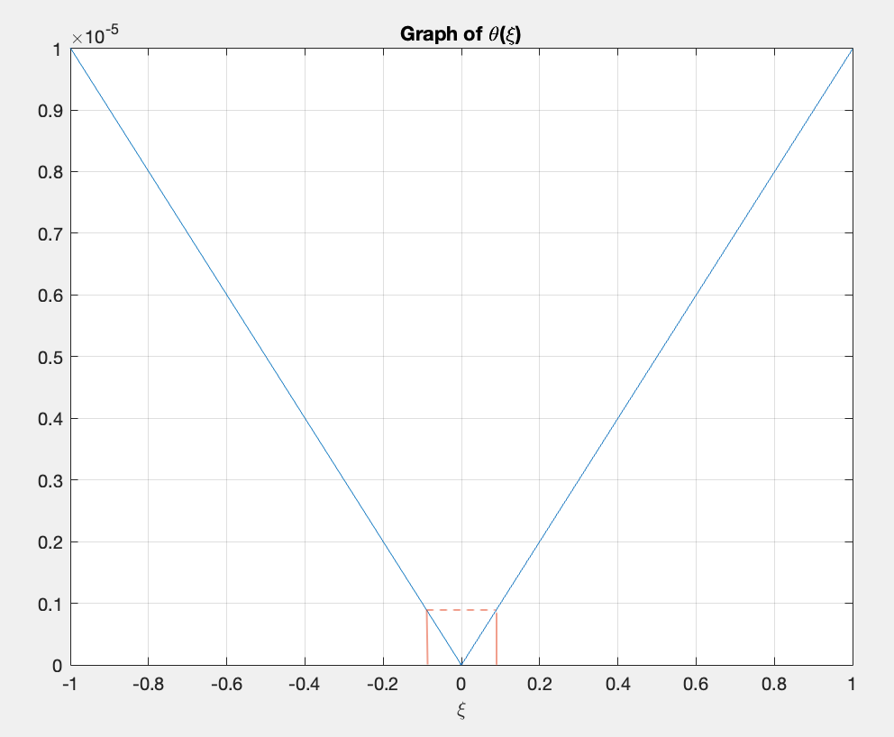
We need to make sure that the infinitesimal action of along the orbit of over induces a horizontal translation on by escaping the vertical cone (see Figure 1 above). To achieve this, it is necessary that does not belong to . The worst case scenario occurs when implying that is . This means that the infinitesimal generator tends to force move away from a suitable at leats for times near . We need to guarantee that indeed we can choose a narrow cone such that all vectors inside leave the cone in a small fraction of time, making use of the effort in the horizontal given by the infinitesimal generator.
Let us choose small enough such that for all
| (18) |
where the minimum is taken over all the possible combinations of signs. We have
∎
Remark 4.6.
Notice that if we consider very small, then from the proof of Lemma 4.5 if is such that , then we also have .
4.4. Conservative kinetic rotations
We start by introducing a simple example where we can observe the flavour of a kinetic rotation seen as an action on a fixed fiber.
Example 4.7.
(shear matrix) The fundamental solution of the autonomous linear variational equation , where
and , is given by the shear matrix
with shear parallel to the axis. Notice that from the linear variational equation we get . The single eigenvalue of is with eigenvector which is a saddle-node fixed point in the projective space . If (respectively ) the dynamics in the projective space is a counter-clockwise ‘rotation’ (respectively clockwise) except of course the direction fixed direction (see Figure 2). The angle between a vector and its image under decreases to 0 as we get close to the vertical direction inside a cone , and is bounded away from 0 outside the cone. Indeed, take where , that is . Then, . Clearly, when and for a fixed when .
We are interested in producing a perturbation of composition type.
| (19) |
which is somehow related to the equality appearing in Definition 4.1 because
So the next result (cf. Lemma 4.10) takes care to consider simultaneously three key aspects for a perturbation: is kinetic, is frictionless and will allow a composition type perturbation.
Definition 4.8.
Let be given and . For all and we define
satisfying
| (20) |
Remark 4.9.
Notice that fixing , and a non-periodic and defining
| (21) |
we have and for we have .
Lemma 4.10.
Proof.
Notice that is the perturbation of by supported on . That (respectively ) follows from Definition 4.8 and Remark 4.9.
Noticing that we get by integrating by parts
and so
Moreover we also have
and so (22) follows from uniqueness of solutions of a linear integral equation
when fixed the initial condition, and the lemma is proved.
∎
4.5. Proving accessibility
We start by showing that, for small, the action on a fixed fiber given by the solution of , provides a rotational behavior stronger than the action of the solution of , for a suitable constant .
Lemma 4.11.
Let , and . There exist and such that for and we have
| (23) |
and
| (24) |
where
is the solution of the linear variational equation for defined as in (20) and is the solution of the linear variational equation .
Proof.
We begin by considering Lemma 3.3 and choose such that (23) holds. Recall the definitions of and in (20). Now, for the angle is defined by
| (25) |
∎
We are now in conditions to achieve accessibility for kinetic cocycles. As highlighted at the outset of Section 4.3, our first step involves selecting a vertical cone . On one hand, this cone presents challenges for rotation, yet on the other hand, the original cocycle swiftly displaces vectors from the cone in time less than (cf. Lemma 4.5). Once vectors exit the cone, we can engineer a suitable perturbation to redirect one direction into another (cf. Lemma 4.10 for rotation and Lemma 4.11 for selecting an appropriate time ). This manipulation relies on a map as defined in Definition 4.8, which operates effectively only outside the vertical cone . Overall, we are well-positioned to implement perturbations that facilitate accessibility, confined within time-1 segments of the orbit. This constitutes our next result.
Lemma 4.12.
Let and . There exists such that if is a -generic point and belong to such that , then there is a perturbation of supported on such that
-
(i)
, for all and
-
(ii)
if and we have .
Proof.
Let be given and . Consider any . By Lemma 4.5 there exists such that given any and we have .
Let us consider two cases:
Case 1: If are such that , then we take from Definition 4.8 and by Lemma 4.10 the cocycle defined by belongs to , where
| (26) |
Moreover, for , we have . Therefore, we can perform the required rotation by tuning appropriately to get
| (27) |
| (28) |
From (26) we get
| (29) |
and (ii) holds.
Case 2:
Remark 4.13.
Lemma 4.12 also holds for the frictionless (respectively dissipative) case, because given (respectively ), the perturbation is obtained by considering where and is traceless, so (respectively ).
Remark 4.14.
We may extend the previous perturbations from a segment of the orbit to a flowbox , , with no self-intersections, when we have attached a pair of unit vectors for all .
Finally, we obtain:
Proposition 4.15.
The families of kinetic cocycles in the present paper are all accessible.
5. Proof of the theorems
5.1. Proof of the version of Theorem 1
Next results (Lemmas 5.1, 5.2 and 5.3) will be stated for elements in but mutatis mutandis the reader can easily see that work also for and . Before stating the lemmas let us consider several useful sets. Let be given over the flow and a -invariant set . Let be set of regular points provided by Oseledets’ theorem [27] where stand for the points with trivial spectrum and stand for the points with simple spectrum. Fixing we say that has -dominated splitting if for -a.e. the fiber decomposes into two -invariant one-dimensional directions such that:
| (30) |
Let us fix some notation:
-
•
is the set of points in whose orbit display an -dominated splitting.
-
•
.
-
•
and
-
•
.
The set has an -uniformly hyperbolic splitting if for -a.e. the fiber decomposes into two -invariant one-dimensional directions such that:
| (31) |
In [12, Lemma 4.1] was proved that contains no periodic points. Lemma 5.1 bellow is a well-know statement which in rough terms say that in the absent of a dominated splitting and along a large orbit segment we can implement rotations of a tiny angle in order to interchange two given directions. Clearly, we will apply Lemma 4.12 times observing that, as the perturbations have distinct support, the concatenation of these perturbations do not add with respect to the size of the final perturbation.
Let be the set of points such that . Hence, .
Lemma 5.1.
Let be given and . There exists such that for -a.e. there exists supported on the segment and such that
-
(i)
and
-
(ii)
.
The second result says that interchanging directions as provided by Lemma 5.1 is effective when the task is to diminish the norm growth pointwise.
Lemma 5.2.
Let be given , and . If is sufficiently large, then there exists a measurable function such that for -a.e. and every there exists supported on the segment and such that and
| (32) |
Moreover, depends measurably on and continuously on .
Proof.
For full details on the proof we refer [11, 12, 6, 7]. The highlights are the following. We assume that otherwise the proof ends. By Lemma 5.1 if is sufficiently large, then for there exists a perturbation supported on the segment and such that (i) and (ii) . A laborious measure theoretical reasoning (see e.g. [12, Proposition 4.2] or [11, Lemma 3.13]) can be made to obtain a measurable function such that for -a.e. and every , there is such that . The way we build the perturbation is by considering:
| (33) |
where and since for , , we have . If no perturbations were introduced, we would obtain
Once we perform the perturbation like in (33) the exponential rate associated to working on half of the way mixes with the exponential rate associated to working on the other half. This results in the estimate in (32). ∎
The third result, says that interchanging directions provided by Lemma 5.1 is effective when the task is to diminish the norm grow globally. Again a laborious measure theoretical reasoning envolving Kakutani castles do the job (see e.g. [12, Lemma 7.4]). The extrapolation of inequality (34) from (32) is far from being an easy task. Indeed, (34) gives a global information on the Lyapunov exponents while (32) gives only pointwise information on a finite iteration.
Lemma 5.3.
Let be given , and . There exists and , with , and that equals outside the open set , such that
| (34) |
Since by Lemma 3.5 we have that the function (12) is upper semicontinuous and the continuity points of upper semicontinuous functions is a residual subset we only have to check that if is a continuity point of then for -a.e. . Let be an Oseledets regular point for . If the two Lyapunov exponents of at coincide, there is nothing to prove. Otherwise, , and so for some . As a conclusion we have:
Theorem 5.4.
Let be a flow preserving the measure . There exists a residual set , such that if , then for -a.e. either
-
•
there exists a single Lyapunov exponent or else
-
•
the splitting along the orbit of is dominated.
5.2. Proof of Theorem 1
Next result proves that a map in belongs to on nearly all its domain.
Lemma 5.5.
Lusin-type theorem: Let and . There such that
Proof.
By Lusin’s theorem (see e.g [28]) given and there exist compact sets such that , , and . As the intersection of two compact subsets on a Hausdorff space is compact we define . By Tietze extension theorem (see e.g. [25]) we can define and as extensions, respectively, of the continuous functions and . Clearly, defined by
belongs to and we have . ∎
Lemma 5.5 and Theorem 5.4 will imply Theorem 1. The way we use these results is somehow natural and next we present the highlight of the proof of a simple case (Theorem 2). It is well-know that the set of continuity points of an upper semicontinuous function is a residual subset. So we will prove first that if is a continuity point of the upper semicontinuous function (recall Lemma 3.5), then the dichotomy in Theorem 2 holds. The proof is by contradiction assuming that exists a -positive measure set without a dominated splitting and such that . We then use Theorem 5.4 and construct such that and so . Now, Lemma 5.5 allows us to obtain , -arbitrarily close to (thus close to ) and such that we still have which draw in a contradiction with the assumption the was a continuity point of . Here, means that we can cause a discontinuity on the map .
5.3. Proof of Theorem 2 and Theorem 3
To prove Theorem 2 we notice that our perturbations keep us inside . As for -a.e. the version of Lemma 5.3 will be as follows: Let be given , and . There exists and with that equals outside the open set and such that . To get the version of our result we use a similar reasoning like in Lemma 5.5.
To prove Theorem 3 we use again the perturbations developed in §4 to rotate solutions and remain inside . Now, the version of Lemma 5.3 will be as follows: Let be given , and . There exists and that equals outside the open set , with , and such that (34) holds. Again on we get the first item of Theorem 3 i.e. the solution of almost every equation (1) is stable or equivalently, for -a.e. the exists a single negative Lyapunov exponent. Otherwise we have -a.e. for some . From Oseledets’ theorem and Liouville’s formula we get:
Now, we have two possible situations: the solution of every associated equation (1) is stable (dominated splitting with two negative Lyapunov exponents) or else the solution of every associated equation (1) displays a dominated splitting with two Lyapunov exponents of different signs. Hence, for any initial condition in the complement of the Oseledets direction associated to the negative Lyapunov exponent the solution of every associated equation (1) is uniformly unstable which is precisely the last item of Theorem 3.
5.4. Theorem 2 applied to the 1-d Schrödinger case
Finally, we present traceless continuous-time linear cocycles with a somewhat different look, namely by considering the one-dimensional Schrödinger operator on and with an potential given by:
| (35) |
In particular we like to describe the Lyapunov spectrum of the time-independent Schrödinger equation
| (36) |
where is a given energy. Putting together (35) and (36) we deduce a kinetic cocycle as in (11) but with and for all . We fix the energy and focus on the continuous-time linear cocycle
called 1-d Schrödinger LDS with potential .
Let stand for the set of continuous potentials. As a direct consequence of Theorem 2 we have:
Theorem 4.
Let be a flow preserving the measure and fix the energy . There exists a residual set , such that if , then for the 1-d Schrödinger continuous-time linear cocycle with energy and potential either
-
•
all Lyapunov exponents vanishes or else
-
•
the splitting along the orbit of is uniformly hyperbolic.
Acknowledgements: MB was partially supported by CMUP, which is financed by national funds through FCT-Fundação para a Ciência e a Tecnologia, I.P., under the project with reference UIDB/00144/2020. MB was also partially supported by the project Means and Extremes in Dynamical Systems PTDC/MAT-PUR/4048/2021. HV was partially supported by FCT - ‘Fundação para a Ciência e a Tecnologia’, through Centro de Matemática e Aplicações (CMA-UBI), Universidade da Beira Interior, project UIDB/MAT/00212/2020.
References
- [1] D. Amaro, M. Bessa, H. Vilarinho, Genericity of trivial Lyapunov spectrum for -cocycles derived from second order linear homogeneous differential equations, J. Differ. Equ., 380 (2024) 228–253.
- [2] D. Amaro, M. Bessa, H. Vilarinho, Simple Lyapunov spectrum for linear homogeneous differential equations with parameters. Nonlinear Differ. Equ. Appl. 31, 43 (2024).
- [3] L. Arnold, Random Dynamical Systems, Springer Verlag, 1998.
- [4] L. Arnold, H. Crauel, J.-P. Eckmann, editors Lyapunov Exponents. Proceedings, Oberwolfach 1990, volume 1486 of Springer Lecture Notes in Math. Springer-Verlag, Berlin Heidelberg New York, 1991.
- [5] L. Arnold, V. Wihstutz, editors, Lyapunov Exponents. Proceedings, Bremen 1984, volume 1186 of Springer Lecture Notes in Mathematics. SpringerVerlag, Berlin Heidelberg New York, 1986.
- [6] M. Bessa, Dynamics of generic 2-dimensional linear differential systems, J. Differ. Equ., 228 (2) (2006) 685–706.
- [7] M. Bessa, Dynamic of generic multidimensional linear differential systems, Advanced Nonlinear Studies 8 (2008) 191–211.
- [8] M. Bessa, Perturbations of Mathieu equations with parametric excitation of large period, Advances in Dynamical Systems and Applications, 7, 1, (2012) 17–30.
- [9] M. Bessa, Lyapunov exponents for linear homogeneous differential equations, In: Dias, J.L., et al. New Trends in Lyapunov Exponents. NTLE 2022. CIM Series in Mathematical Sciences. Springer.
- [10] M. Bessa, H. Vilarinho, Fine properties of -cocycles which allows abundance of simple and trivial spectrum. J. Differ. Equ., 256, 7 (2014) 2337–2367.
- [11] J. Bochi, Genericity of zero Lyapunov exponents, Ergod. Th. & Dynam. Sys. 22 (2002) 1667–1696.
- [12] J. Bochi, M.Viana, The Lyapunov exponents of generic volume-preserving and symplectic maps, Ann. of Math. 161 (3) (2005) 1423–1485.
- [13] N. D. Cong, D. T. Son, On integral separation of bounded linear random differential equations, Discrete and Continuous Dynamical Systems - S. (2016),9(4), 995-1007.
- [14] R. Fabbri, Genericity of hyperbolicity in linear differential systems of dimension two, (Italian) Boll. Unione Mat. Ital., Sez. A, Mat. Soc. Cult. 8 (1) Suppl. (1998) 109–111.
- [15] R. Fabbri, On the Lyapunov Exponent and Exponential Dichotomy for the Quasi-Periodic Schrödinger Operator, Boll. Unione Mat. Ital. 8 (5-B) (2002) 149–161.
- [16] R. Fabbri, R. Johnson, Genericity of exponential dichotomy for two-dimensional differential systems, Ann. Mat. Pura Appl. IV. Ser. 178 (2000) 175–193.
- [17] R. Fabbri, R. Johnson, On the Lyapounov exponent of certain SL-valued cocycles, Differ. Equ. Dyn. Syst. 7 (3) (1999) 349–370.
- [18] R. Fabbri, R. Johnson, L. Zampogni, On the Lyapunov exponent of certain SL-valued cocycles II, Differ. Equ. Dyn. Syst. 18 (1-2) (2010) 135–161.
- [19] X. Feng, K. Loparo, Almost sure instability of the random harmonic oscillator, SIAM J. Appl. Math. 50, 3, (1990) 744–759.
- [20] R. Johnson, K. Palmer, G. Sell, Ergodic properties of linear dynamical systems, SIAM J. Math. Anal. 18 (1987) 1–33.
- [21] A. Leizarowitz, On the Lyapunov exponent of a harmonic oscillator driven by a finite-state Markov process, SIAM J. Appl. Math., 49, 2, (1989) 404–419.
- [22] R. Mañé, Oseledec’s theorem from generic viewpoint, Proceedings of the international Congress of Mathematicians, Warszawa vol. 2 (1983) 1259–1276.
- [23] R. Mañé, The Lyapunov exponents of generic area preserving diffeomorphisms, International Conference on Dynamical Systems (Montevideo, 1995), Pitman Res. Notes Math. Ser. 362 (1996) 110–119.
- [24] V. M. Millionshchikov, Systems with integral separateness which are dense in the set of all linear systems of differential equations, Differential Equations 5 (1969) 850–852.
- [25] J. R. Munkres, Topology: A First Course, Prentice-Hall, Inc. 1975.
- [26] V. L. Novikov, Almost reducible systems with almost periodic coefficients, Mat. Zametki 16 (1974) 789–799.
- [27] V. Oseledets, A multiplicative ergodic theorem: Lyapunov characteristic numbers for dynamical systems, Transl. Moscow Math. Soc. 19 (1968) 197-231.
- [28] W. Rudin, Real and Complex Analysis, 3rd ed., Mc Graw Hill, International Edition 1987.