Joint-Task Regularization for Partially Labeled Multi-Task Learning
Abstract
Multi-task learning has become increasingly popular in the machine learning field, but its practicality is hindered by the need for large, labeled datasets. Most multi-task learning methods depend on fully labeled datasets wherein each input example is accompanied by ground-truth labels for all target tasks. Unfortunately, curating such datasets can be prohibitively expensive and impractical, especially for dense prediction tasks which require per-pixel labels for each image. With this in mind, we propose Joint-Task Regularization (JTR), an intuitive technique which leverages cross-task relations to simultaneously regularize all tasks in a single joint-task latent space to improve learning when data is not fully labeled for all tasks. JTR stands out from existing approaches in that it regularizes all tasks jointly rather than separately in pairs—therefore, it achieves linear complexity relative to the number of tasks while previous methods scale quadratically. To demonstrate the validity of our approach, we extensively benchmark our method across a wide variety of partially labeled scenarios based on NYU-v2, Cityscapes, and Taskonomy.
1 Introduction
In recent years, multi-task learning (MTL) has gained popularity in the field of machine learning. This approach involves training a model to perform multiple related tasks simultaneously, as opposed to traditional machine learning methods which train multiple independent models for each task. By leveraging commonalities across tasks, multi-task learning has the potential to improve overall performance while reducing inefficiencies and redundancies in the learning process. In particular, dense prediction tasks such as semantic segmentation and depth estimation have been particularly promising areas for multi-task learning, as these tasks typically require large models and significant computational resources. Extensive research has been conducted in various directions to achieve effective multi-task learning [9, 51, 32, 61], including architecture design [44, 52, 6, 41, 27, 7, 59] and optimization strategies [30, 22, 66, 12, 71, 46]. While these studies have demonstrated the effectiveness of multi-task learning, their applicability is limited by data availability. Training multi-task models requires high quality data, which is often expensive and time-consuming to acquire.
Collecting data for multi-task learning presents two primary challenges. The first challenge is the cost of annotating dense labels. For instance, annotating a segmentation mask for a single image in the Cityscapes dataset took over 1.5 hours on average [17]. Single task semi-supervised learning presents a potential solution to this problem—however, despite extensive research on semi-supervised learning [4, 43, 47, 25], its application to multi-task learning remains underexplored. Second, for tasks which involve predicting other modalities from images (such as depth or surface normal estimation), obtaining data introduces the challenge of sensor alignment and synchronization, requiring an expensive sensor fusion system. Building a sensor fusion system with high quality calibration and synchronization is difficult and necessitates specialized research. [70]. One way to overcome this problem is to collect data for various subsets of tasks in a particular domain and train a model to perform all of the tasks jointly. However, multi-task learning without fully labeled data requires dealing with partial supervision, as each data sample is labeled for different tasks. Previous works have attempted this form of partial supervision for multi-task models in multiple ways: for instance, single-task semi-supervised learning methods regularize models through feature or output consistency with perturbed inputs for unlabeled tasks [29, 57, 48, 19, 21]. While these approaches supplement the lack of supervision, they do not fully utilize the underlying cross-task relationships which are present in multi-task learning. To remedy this issue, recent pair-wise multi-task methods perform regularization across every pair of labeled and unlabeled tasks [73, 62, 58, 74]. While such methods have shown promising results, their performance and poor scalability due to their quadratic complexity leaves much to be desired.
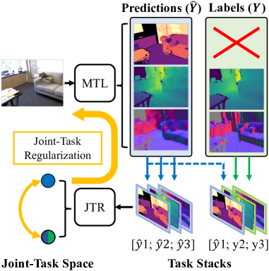
To this end, we propose a new approach for achieving data-efficient multi-task learning using partially labeled data. Our method, Joint-Task Regularization (JTR), encodes predictions and labels for multiple tasks into a single joint-task latent space. The encoded features are then regularized by a distance loss in the joint-task latent space, propagating gradients through all task branches at once. Our approach has two main advantages: first, information flows across multiple tasks during regularization with backpropagation through a learned encoder, yielding a better metric space than naive spaces such as pixel-wise Euclidean or cosine distance. Second, our method scales favorably relative to the numbers of tasks at hand. Unlike previous methods which regularize tasks in a pair-wise fashion [73, 62, 58, 74], JTR has linear complexity—this gives JTR a notable advantage in datasets with a large number of tasks over pair-wise task regularization methods which scale quadratically.
In our experiments, we demonstrate the effectiveness of our method on variations of three popular multi-task learning benchmarks, namely NYU-v2, Cityscapes, and Taskonomy. We also conduct additional performance comparisons and ablation studies to inspect JTR’s key characteristics.
To summarize, our main contributions are as follows:
-
•
We investigate the underexplored problem of label-efficient multi-task learning with partially labeled data.
-
•
We propose JTR, a model-agnostic technique which introduces a joint-task space to regularize all tasks at once.
-
•
We extensively benchmark JTR on the NYU-v2, Cityscapes, and Taskonomy datasets to demonstrate its advantages over the current state-of-the-art.
2 Related Works
Multi-Task Learning
Multi-task learning aims to improve models’ performance and generalization capabilities on individual tasks by exploiting commonalities and interdependencies between tasks through shared representations. Several methods have been proposed to achieve effective multi-task learning through architectural modifications. For example, [44, 52, 6, 15, 11] use multiple task experts and interconnect them to allow information and representation learning to flow across multiple tasks. Meanwhile, [41, 27, 7, 59, 75, 16, 1] adopt a strategy which gradually expands the depth of the model being trained, allowing the network to learn task-specific representations in a more resource efficient manner. Various other techniques have been proposed for multi-task learning, including the attention mechanism [77, 38, 8], knowledge distillation [67, 60, 21], task pattern propagation [78, 79], generative models [3], and transformers [68, 69, 20]. Another line of work tackles multi-task learning from an optimization perspective. Numerous optimization techniques have been proposed: some examples include loss weighting [30, 22, 66], gradient normalization [12], gradient dropout [13], gradient surgery [71], Nash Bargaining solutions [46], Pareto-optimal solutions [54, 35, 45], gradient alignment [55], and curriculum learning [26, 28]. Recently, with the rise of large-scale models and the pretrain-finetune paradigm, adapter-based multi-task finetuning methods [34, 40] have also been introduced. Although extensive studies have been conducted on multi-task learning, these methods still require fully supervised training data which is difficult to obtain in practical scenarios due to high costs.
Partially Labeled Multi-Task Learning
The advent of multi-task learning with partially labeled data has received limited attention in existing literature. Early works focused on multi-task learning with shallow models by employing parameter sharing [37, 76] or convex relaxation [63]. More recently, several studies have tackled multi-task learning with missing labels based on deep models. For instance, Chen et al. [14] propose to use a consistency loss across complementary tasks such as shadow edges, regions, and counts to tackle a shadow detection problem by leveraging unlabeled samples. However, this method is limited to tasks which have explicit connections to each other. Others have attempted more general multi-task learning with partially labeled data with techniques such as domain discriminators [64] and cross-task regularization by joint pair-wise task mappings [33]. Furthermore, an orthogonal work by Borse et al. [5] adds an auxiliary conditional regeneration objective to MTPSL [33] to improve performance.
Although these approaches address multi-task learning with partially labeled data, their performance leaves much to be desired. Additionally, existing methods are often challenging to implement in practice and scale poorly to larger datasets with many tasks. For example, MTPSL [33] incorporates FiLM [50] in an effort to offset its quadratic complexity, but this introduces additional hyperparameters, architecture-level modifications, and optimizers to the training process. In this work, we investigate a new avenue for achieving effective multi-task learning without compromising on simplicity and scalability.
Cross-Task Relations
Given that different visual perception tasks are often correlated with each other [73, 72], there is growing interest in exploring cross-task relations [36, 42, 74, 24, 33]. For example, Taskonomy [73] exposes relationships among different visual tasks and models the structure in a latent space. Cross-task relations have also been exploited for domain adaptation [49, 74, 53], and cross-task consistency learning [74] attains better generalization to out-of-distribution inputs. Saha et al. [53] propose a cross-task relation layer to encode task dependencies between the segmentation and depth predictions, and successfully improve model performance in an unsupervised domain adaptation setting. Some studies utilize cross-task relations to improve the performance of a single task [10, 24]. Guizilini et al. [24] leverage semantic segmentation networks for self-supervised monocular depth prediction. Cross-task consistency is also extensively investigated in MTL. Taskology [42] designs a consistency loss to enforce the logical and geometric structures of related tasks, reducing the need for labeled data. Most relevant to our work, Li et al. [33] leverage task relations by mapping each task pair to a joint pair-wise task space for multiple dense prediction tasks on partially annotated data. In this work, we propose a simple and scalable approach to perform regularization in a joint-task space by leveraging implicit cross-task relations.
3 Method
3.1 Definitions
Let be the set of all task indices where is the number of tasks. We define as the set of training samples for tasks. For each training image , let and be the sets containing indices of tasks which are labeled and unlabeled, respectively (such that ). Let denote a RGB input image in , and let its corresponding dense label for task be denoted by where is the number of output channels for task . As is standard in MTL literature [30, 12, 54], we seek to fit a common backbone feature extractor parameterized by where , , are the channel, height, and width of the extracted feature map, respectively (where typically and ). We also seek to fit multiple task-specific decoders , each separately parameterized by task-specific weights . For each target task , the model’s prediction can be expressed as . We also denote any variable with detached gradients using angular brackets.
3.2 Baselines for MTL with Partially Labeled Data
Supervised Multi-Task Learning
A naïve way to fit for all tasks is to optimize parameters and for all labeled tasks for all items in the training dataset as follows:
| (1) |
where is a differentiable loss function for a specific task . Here, weights for the backbone feature extractor are learned using all labeled images while task-specific weights for each task are only learned for dataset examples which are labeled for task ().
SSL with Consistency Regularization
One common strategy to improve upon naïve supervised learning is to apply Semi-Supervised Learning (SSL). In particular, Consistency Regularization (CR) is a common method of leveraging data augmentation to encourage models to output consistent predictions across multiple different augmentations of unlabeled data [29, 57, 48, 19]. More concretely, Eq. 1 is modified as follows:
| (2) |
where is an unsupervised loss function (e.g. L2 loss) and is a function which applies augmentation to an image . We recognize that there are more advanced SSL methods which exploit task-specific properties such as SSL for semantic segmentation [43, 47] and depth estimation [25] in single-task learning settings. However, it is commonly understood that applying pseudo-labeling methods in multi-task settings is a major challenge because most semi-supervised loss functions are designed based on task-specific properties, and it is unclear how to effectively combine them when working with multiple tasks simultaneously [33]. Therefore, following previous works, we primarily use Consistency Regularization as the baseline SSL method throughout this work (for completeness, we also benchmark SSL with pseudo-labels in Sec. 4.5).
Pair-Wise Task Relations
While Eq. 2 indeed incorporates partially labeled data for training, it does not leverage implicit relationships and commonalities between tasks. To exploit such potentially useful task relationships, some previous works have proposed to learn pair-wise mappings or construct explicit graph connections between pairs of tasks [73, 62, 58, 74]. Most relevant to our work is MTPSL [33] which creates a “mapping space” for each pair of tasks. Using these task pair-wise mapping spaces, MTPSL seeks to maximize the similarity of an unlabeled task prediction “mapped” to a labeled task as follows:
| (3) |
where is the cosine distance function (), is a learned mapping function (typically an encoder similar to ), and each is a set of parameters which parameterizes . MTPSL additionally incorporates FiLM [50] to reduce number of parameters required for parameterizing for each task pair . However, because is still computed for task pairs, MTPSL suffers from quadratic complexity and is unable to leverage information which may arise from relationships among more than tasks.
3.3 Joint-Task Regularization (JTR)
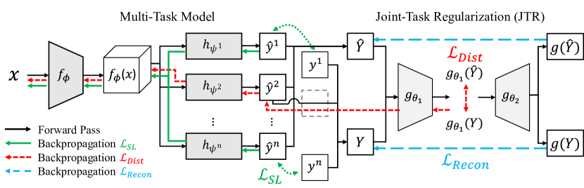
To remedy the aforementioned issues with pair-wise mapping schemes like MTPSL, JTR completely avoids modeling task relations in pairs by instead learning a regularization space as a single function of all tasks. More concretely, for each input image and corresponding label , we generate a noisy prediction tensor by stacking predictions () for all tasks along the channel dimension. Then, we create a reliable target tensor by stacking labels () if task is labeled, using predictions () as a substitute when no label exists for task . Formally, let and be defined as follows:
| (4) |
where . The shapes of and are , where is the number of channels for task . Then, we define the JTR encoder-decoder as . Here, and for some . We call the output space of the “joint-task space,” since it represents information about all tasks at once. In this setup, forms an auto-encoder architecture which encodes and reconstructs and across the joint-task space as the bottleneck, preventing the encoder from learning a trivial joint-task space. Now, we can define a loss term to minimize the distance between and in the joint-task space while also fitting and :
| (5) |
Here, the joint latent distance loss is some distrance metric (e.g. the cosine distance function ), and measures the quality of the decoder’s reconstruction using the task-specific loss functions for all tasks . We also detach the terms’ gradients to prevent the model from outputting degenerate predictions to trivialize the reconstruction task. An illustration of these components of JTR is provided in Fig. 2.
Now, we can sum the supervised loss and the JTR loss term from Eq. 5 to get the following optimization objective:
| (6) |
where is the supervised loss in Eq. 1.
Since and aggregate predictions and labels for all tasks into a single representation, JTR’s distance loss term in the joint-task space propagates gradients to all tasks jointly. This has both performance and efficiency benefits: for one, JTR is able to leverage relationships which may arise from non-obvious combinations of tasks, giving it an advantage over existing methods which only model inter-task dependencies by pairs [73, 62, 58, 74]. Second, JTR achieves linear complexity with respect to the number of tasks, differentiating itself from existing methods which scale quadratically. As our experiments show in the following section, these benefits allow JTR to perform significantly more favorably than existing methods in a variety of partially labeled multi-task learning settings.
4 Experiments
4.1 Experimental Setup
To benchmark JTR against existing partially labeled MTL methods, we conduct experiments on three common multi-task dense prediction benchmarks: namely NYU-v2 [56, 38], Cityscapes [17], and Taskonomy [73]. These public research datasets are intended for benchmarking purposes, so each data sample is fully labeled for all tasks. To simulate more realistic partially labeled scenarios, we follow [33] in synthetically generating “randomlabels” and “onelabel” settings for all three datasets. Throughout our work, “randomlabels” means each dataset example has a random number of labels between and at most (where is the number of tasks), while “onelabel” means each example has exactly one label for a randomly chosen task. For the Taskonomy benchmark, we follow previous works [58] in training multi-task models on seven tasks: semantic segmentation, depth, surface normals, edge occlusions, reshading, 2D keypoints, and edge textures. Additionally, we introduce one more partially labeled setting named “halflabels” for the Taskonomy experiment. In “halflabels,” each dataset sample has or labels out of tasks. This is a more balanced partially labeled setting than the “randomlabels” setting, while the mean number of labels in both settings is the same. The Taskonomy experiments are conducted using the ‘Tiny’ dataset split.
We base the implementation of JTR (as well as all baselines) on the public code repository provided by Li et al. [33, 23]. Across all experiments, we use SegNet [2] as the MTL backbone. For JTR, we use the same SegNet architecture as the MTL backbone with only the input and output channel dimensions modified as needed. We also use the SegNet architecture for the “Direct Cross-Task Mapping” and “Perceptual Cross-Task Mapping” baselines as formulated by Li et al. [33] and Zamir et al. [74]. We use cross-entropy loss for semantic segmentation, L1 norm loss for depth estimation, and cosine similarity loss for surface normal estimation. For the four additional tasks in the Taskonomy experiment, we use L1-norm loss following Standley et al. [58]. Additionally, we apply RandAugment [18] across our experiments. We use mostly identical hyper-parameters including the learning rate and the optimizer as the code for MTPSL [33, 23] (see Supplementary Material for more details). For evaluation metrics, we use mean intersection over union (mIoU), absolute error (aErr), and mean angle error (mErr) for semantic segmentation, depth estimation, and surface normal estimation tasks, respectively. For the four additional tasks in Taskonomy, we use absolute error (aErr). We also report the mean percentage “improvement” (relative performance increase or relative error decrease) of each benchmarked method over the corresponding multi-task Supervised MTL baseline (averaged across all tasks) as “.”
| Method | Seg. | Depth | Norm. | |
| fully labeled | ||||
| Supervised MTL* | 38.91 | 0.5351 | 28.57 | — |
| onelabel | ||||
| Supervised MTL* | 25.75 | 0.6511 | 33.73 | +0.000 |
| Consistency Reg.* | 27.52 | 0.6499 | 33.58 | +2.501 |
| Direct Map* [74] | 19.98 | 0.6960 | 37.56 | –13.55 |
| Perceptual Map* [74] | 26.94 | 0.6342 | 34.30 | +1.842 |
| MTPSL [33] | 30.40 | 0.5926 | 31.68 | +11.04 |
| Ours (JTR) | 31.96 | 0.5919 | 30.80 | +13.97 |
| depth-extended “onelabel” | ||||
| Supervised MTL | 23.43 | 0.6918 | 39.44 | –10.73 |
| Consistency Reg. | 23.94 | 0.6840 | 40.12 | –10.34 |
| MTPSL [33] | 33.80 | 0.4794 | 37.50 | +15.49 |
| Ours (JTR) | 33.63 | 0.4898 | 31.37 | +20.79 |
| randomlabels | ||||
| Supervised MTL* | 27.05 | 0.6624 | 33.58 | +0.000 |
| Consistency Reg.* | 29.50 | 0.6224 | 33.31 | +5.300 |
| Direct Map* [74] | 29.17 | 0.6128 | 33.63 | +5.060 |
| Perceptual Map* [74] | 32.20 | 0.6037 | 32.07 | +10.80 |
| MTPSL [33] | 35.60 | 0.5576 | 29.70 | +19.66 |
| Ours (JTR) | 37.08 | 0.5541 | 29.44 | +21.92 |
| Scenario | Method | Seg. | Depth | |
| fully labeled | Supervised MTL* | 72.70 | 0.0163 | — |
| onelabel | Supervised MTL* | 69.50 | 0.0186 | +0.000 |
| Consistency Reg.* | 71.67 | 0.0178 | +3.712 | |
| MTPSL [33] | 72.09 | 0.0168 | +6.702 | |
| Ours (JTR) | 72.33 | 0.0163 | +8.219 |
| Scenario | Method | Seg. | Depth | Norm. | Occl. | Resh. | KeyP. | Text. | |
| onelabel | Consistency Reg. | +0.080 | +6.106 | +4.957 | +1.124 | +3.905 | –8.723 | +17.63 | +1.567 |
| MTPSL [33] | +0.646 | +4.172 | +6.201 | +0.829 | +7.540 | –11.75 | +23.94 | +1.973 | |
| Ours (JTR) | +0.381 | +8.477 | +6.236 | +1.076 | +6.223 | –1.222 | +35.03 | +3.512 | |
| randomlabels | Consistency Reg. | –0.058 | +8.438 | +1.218 | +0.531 | +4.460 | +6.622 | +14.86 | +2.254 |
| MTPSL [33] | +0.311 | +17.70 | +2.355 | +1.349 | +10.08 | –20.68 | +9.771 | +1.261 | |
| Ours (JTR) | +0.193 | +12.14 | +9.061 | +2.030 | +9.740 | +1.955 | +30.40 | +4.095 | |
| halflabels | Consistency Reg. | +0.578 | +4.173 | +5.884 | +1.252 | +4.493 | +11.43 | +9.415 | +2.326 |
| MTPSL [33] | +0.656 | +7.723 | +10.49 | +2.496 | +9.100 | +0.552 | +19.55 | +3.160 | |
| Ours (JTR) | +0.776 | +11.05 | +13.28 | +3.055 | +10.98 | +9.442 | +32.62 | +5.075 |
4.2 Partially Labeled MTL
NYU-v2
We present our results with NYU-v2 under the “onelabel” and “randomlabels” settings in Tab. 1. We observe that in both scenarios, JTR convincingly outperforms existing methods across all three tasks. Note that results marked * are quoted from [33] to maintain consistency with results from previous works (for more details, please see our explanation of “Copied Baselines” in Sec. 6.3).
Cityscapes
We evaluate our method on Cityscapes under the “onelabel” setting in Tab. 2. Similarly to our results with NYU-v2, JTR outperforms baseline methods across both segmentation and depth estimation tasks. One point to note is that the differences in performance between methods on Cityscapes is less prominent than on NYU-v2, suggesting that Cityscapes is a much less challenging dataset for partially labeled MTL. Nevertheless, JTR comfortably outperforms existing methods on all Cityscapes tasks.
Taskonomy
We present our results using Taskonomy in three partially labeled settings in Tab. 3. In this dataset, consistency regularization, MTPSL and JTR improve upon naïve Supervised MTL. Notably, the consistency regularization baseline and MTPSL enhance overall performance but compromise certain tasks to improve others. For example, the keypoint detection task suffers from large negative effects in the ‘onelabel’ scenario. In contrast, JTR enhance overall performance without large detriments to individual task performance metrics. Our experiments indicate that some form of cross-task regularization is essential to prevent models from biasing for or against specific tasks.
JTR’s margins of improvement on Taskonomy, while noticeable, are not as significant as with NYU-v2 and Cityscapes. This could be attributed to the larger scale of the Taskonomy dataset, which enhances the performance of the supervised baseline. Nonetheless, JTR is more effective in improving the overall MTL performance under different partially labeled scenarios than the competing methods. Additionally, our method holds a significant advantage in terms of computational resource efficiency (further explained in Sec. 4.5).
4.3 Depth-Extended NYU-v2
In addition to the fully labeled images in multi-task NYU-v2, there are an additional samples in the original NYU v2 dataset which are only labeled for the depth estimation task [56, 65]. This is dataset is approximately times larger than the training split of multi-task NYU-v2. To leverage this additional data, we combine the training splits of two datasets to curate a new split named “depth-extended multi-task NYU-v2.” In the context of our experimental setup, this is equivalent to the “onelabel” scenario—therefore, we can leverage this extra data by simply extending the “onelabel” split. This setup puts each method’s resilience to task imbalance to the test.
Our results are presented in Tab. 1 alongside the NYU-v2 “onelabel” results for direct comparison. We can notice that the inclusion of extra depth data has a negative effect on Supervised MTL and Consistency Reg. across all tasks (including depth estimation), highlighting the brittleness of naïve training to task imbalances. For MTPSL and JTR, both outperform their standard “onelabel” counterparts in the segmentation and depth tasks, with MTPSL having a slight edge. However, MTPSL performs very poorly in the surface normal estimation task while JTR maintains comparable performance, yielding a significantly better overall score. These results show that JTR is highly resilient in scenarios with task imbalances (even without additional task-weighting tricks), underscoring the stability and practicality of our approach.
| Method | Seg. | Depth | Norm. | |
| 70% randomlabels + 30% unlabeled | ||||
| Supervised MTL | 26.36 | 0.6574 | 33.02 | +0.000 |
| Consistency Reg. | 29.89 | 0.6136 | 31.93 | +7.785 |
| MTPSL [33] | 31.92 | 0.6071 | 31.59 | +11.03 |
| Ours (JTR) | 32.20 | 0.5912 | 31.01 | +12.77 |
| 50% randomlabels + 50% unlabeled | ||||
| Supervised MTL | 23.68 | 0.6988 | 35.00 | +0.000 |
| Consistency Reg. | 25.16 | 0.6543 | 32.54 | +6.549 |
| MTPSL [33] | 28.18 | 0.6393 | 33.04 | +11.04 |
| Ours (JTR) | 28.69 | 0.6268 | 31.52 | +13.80 |
| 30% randomlabels + 70% unlabeled | ||||
| Supervised MTL | 18.57 | 0.7288 | 37.49 | +0.000 |
| Consistency Reg. | 20.60 | 0.7135 | 34.81 | +6.727 |
| MTPSL [33] | 23.33 | 0.6952 | 34.81 | +12.46 |
| Ours (JTR) | 24.05 | 0.6945 | 34.25 | +14.29 |
| Scenario | Method | Seg. | Depth | |
| 70% onelabel, 30% unlabeled | Supervised MTL | 69.62 | 0.0180 | +0.000 |
| Consistency Reg. | 69.65 | 0.0171 | +2.522 | |
| MTPSL [33] | 71.48 | 0.0169 | +4.391 | |
| Ours (JTR) | 71.07 | 0.0161 | +6.319 | |
| 50% onelabel, 50% unlabeled | Supervised MTL | 67.56 | 0.0196 | +0.000 |
| Consistency Reg. | 69.23 | 0.0174 | +6.848 | |
| MTPSL [33] | 70.30 | 0.0174 | +7.640 | |
| Ours (JTR) | 69.76 | 0.0167 | +9.026 | |
| 30% onelabel, 70% unlabeled | Supervised MTL | 64.65 | 0.0217 | +0.000 |
| Consistency Reg. | 66.43 | 0.0187 | +8.289 | |
| MTPSL [33] | 68.09 | 0.0187 | +9.573 | |
| Ours (JTR) | 67.75 | 0.0179 | +11.15 |
4.4 Partially (Un)labeled MTL
To further test JTR’s capabilities under diverse partial label settings, we generate variants of NYU-v2 and Cityscapes in which a portion of the dataset is randomly chosen to be completely unlabeled, and the remainder is labeled following the aforementioned “randomlabels” or “onelabel” configurations. To enable effective learning learning in these settings, we simply apply consistency regularization in the joint-task latent space when no labels are available. We implement this by making a small modification to Eq. 5 for completely unlabeled samples (i.e. when ):
For both datasets, we created 30% unlabeled, 50% unlabeled, and 70% unlabeled data splits. The labeled portion of the data is kept consistent with the “randomlabels” and “onelabel” scenarios from NYU-v2 “randomlabels” and Cityscapes “onelabel,” respectively. All hyperparameters are kept constant across all unlabeled ratios.
NYU-v2
Results are shown in Tab. 4. In these experiments, all three benchmarked methods improve upon naïve Supervised MTL across all label scenarios. However, JTR consistently outperforms baseline methods across all tasks. Some baselines nearly match JTR in specific tasks—for example, while the difference in depth aErr between MTPSL and JTR in the 70% unlabeled experiment is marginal, JTR handily outperforms MTPSL in the segmentation and normal estimation tasks. Thanks to this ability to better balance multiple tasks, JTR obtains the best overall score. One notable trend is that the score improvement of JTR becomes more pronounced as the level of supervision decreases. This indicates that JTR is effectively taking advantage of its access to unlabeled data to maximize learning.
Cityscapes
Results are shown in Tab. 5. We observe a similar trend with Cityscapes—JTR nearly matches MTPSL’s segmentation mIoU while vastly surpassing all existing methods in depth estimation, and it achieves the highest overall score across every label scenario. While satisfactory, we believe our results in Cityscapes can be further improved by adjusting several parameters to suit the reduction in available data. However, we refrain from varying any hyperparameters as the results already sufficiently demonstrate the efficacy of our approach.
4.5 Additional Results
| Method | SegNet | ResNet-50 | ||
| Time | VRAM | Time | VRAM | |
| MTPSL [33] | 8h 20m | 17.5GiB | 17h 40m | 21.5GiB |
| Ours (JTR) | 9h 00m | 17.5GiB | 10h 50m | 16.2GiB |
| Method | Cityscapes | Taskonomy | ||
| Time | VRAM | Time | VRAM | |
| MTPSL [33] | 22h 10m | 14.4GiB | 223h 10m | 34.4GiB |
| Ours (JTR) | 23h 45m | 19.2GiB | 105h 00m | 23.9GiB |
Computational Costs
The computational cost of JTR is dependent on number of tasks and the size of the encoder/decoder used to learn the joint-task latent space. For small-scale datasets such as NYU-v2 ( tasks) and Cityscapes ( tasks), JTR consumes the same or more resources than MTPSL (Tab. 6, Tab. 7). However, this is due to the “upfront” cost of having the extra encoder/decoder for learning the joint-task latent space. When scaling up to realistic scenarios like Taskonomy ( tasks), JTR gains a monumental advantage over MTPSL in total training time and VRAM usage (Tab. 7). Furthermore, JTR uses less resources than MTPSL when using more typical model architectures like ResNet-50 rather than SegNet (Tab. 6). This gap can be explained by MTPSL’s use of layer-wise FiLM transformations [50], which requires more VRAM for more complex network architectures. We further elaborate on these results in the Supplementary Material.
| Method | Seg. | Depth | Norm. | |
| NYU-v2 “randomlabels” | ||||
| Supervised MTL | 27.05 | 0.6624 | 33.58 | +0.000 |
| MTPSL w/o reg. [33] | 33.51 | 0.5767 | 34.00 | +11.86 |
| MTPSL w/ reg. [33] | 35.60 | 0.5576 | 29.70 | +19.66 |
| JTR w/o | 35.89 | 0.5746 | 32.96 | +15.93 |
| JTR w/ | 37.08 | 0.5541 | 29.44 | +21.92 |
| Cityscapes “onelabel” | ||||
| Supervised MTL | 69.50 | 0.0186 | — | +0.000 |
| MTPSL w/o reg. [33] | 72.27 | 0.0168 | — | +6.832 |
| MTPSL w/ reg. [33] | 72.09 | 0.0168 | — | +6.702 |
| JTR w/o | 71.78 | 0.0166 | — | +7.017 |
| JTR w/ | 72.33 | 0.0163 | — | +8.219 |
Reconstruction Loss
We now present an ablation study on the role of the term which prevents from learning a trivial encoding scheme (i.e. mapping all inputs to a single point) in Tab. 8. As expected, JTR performs more favorably with the inclusion of the term. However, it is worth noting that JTR without still outperforms both naïve Supervised MTL and MTPSL. This indicates that can manage to learn a useful joint-task space even without , and it is consistent with experiments from MTPSL [33] which show that pair-wise task mapping still outperforms naïve Supervised MTL even if the mapping function is not explicitly regularized to prevent trivial solutions (also included in Tab. 8). Given the additional computational costs of (forward and backward passes through the decoder ) and the generally satisfactory performance of JTR without , omitting this term and relying solely on may be worth considering when under severe computational resource limitations.
Teacher-Student Pseudo-Labeling Baseline
In Sec. 3.2, we claim that consistency regularization is a reasonable choice for the baseline semi-supervised MTL method in our experiments, since combining single-task pseudo-labeling techniques for MTL is itself a major challenge [33]. However, for completeness, we also conduct an experiment with the MuST pseudo-labeling framework [21].
MuST is a two-step approach which uses task-specific teacher models and a multi-task student model. When first training the teacher models, MuST uses only labeled samples and performs Single-Task Learning (STL). Then, a student model is trained with pseudo-labels generated by the teacher models for unlabeled tasks. Therefore, MuST performs poorly when labeled portions of the dataset are too small to train good teacher models for each task. This effect can be seen in the Tab. 9: both MTPSL and JTR outperform MuST because the underlying STL teacher models for MuST have subpar performance. Extrapolating from these results, we can infer that MuST’s performance is likely less than the performance of MTPSL [33] in most benchmarks.
| Method | Seg. | Depth | Norm. | |
| Supervised MTL* | 27.05 | 0.6624 | 33.58 | +0.000 |
| Consistency Reg.* | 29.50 | 0.6224 | 33.31 | +5.300 |
| MuST STL Teachers [21] | 24.73 | 0.7278 | 29.78 | –2.378 |
| MuST MTL Student [21] | 30.80 | 0.6185 | 31.82 | +8.577 |
| MTPSL [33] | 35.60 | 0.5576 | 29.70 | +19.66 |
| Ours (JTR) | 37.08 | 0.5541 | 29.44 | +21.92 |
5 Discussion
Limitations
In this work, we investigate multi-task learning in the context of dense prediction tasks. However, applying JTR to MTL models for heterogeneous tasks, i.e. a combination of instance-level classification, regression, and pixel-level dense prediction tasks, may not be straightforward. Extending JTR to arbitrary types of output domains would be an interesting future research direction. Additionally, our experiments are conducted using single-domain data; however, in practical scenarios of MTL with partially labeled data, a more realistic and efficient approach would involve combining existing datasets from heterogeneous domains. This presents a greater challenge as the model needs to address both missing labels and domain gaps, but if successful, this may diversify the applicability of MTL. Lastly, JTR does not take advantage of prior knowledge which can be manually modeled in some datasets. Remedying these limitations may bring further improvements.
Conclusion
In this paper, we propose and demonstrate the effectiveness of applying Joint-Task Regularization (JTR) for multi-task learning with partially labeled data. JTR implicitly identifies cross-task relations through an encode-decode training process and uses this knowledge to regularize the MTL model in a joint-task space. Using variants of NYU-v2, Cityscapes, and Taskonomy, we comprehensively showcase the efficacy and efficiency of JTR in comparison to existing methods across a wide range of partially labeled MTL settings. We believe that JTR is a significant step forward in achieving data-efficient multi-task learning, and we hope that our contributions are helpful for future applications of MTL.
Acknowledgements
We thank all affiliates of the Harvard Visual Computing Group for their valuable feedback. This work was supported by NIH grant R01HD104969.
References
- Aich et al. [2023] Abhishek Aich, Samuel Schulter, Amit K Roy-Chowdhury, Manmohan Chandraker, and Yumin Suh. Efficient controllable multi-task architectures. In IEEE International Conference on Computer Vision, 2023.
- Badrinarayanan et al. [2017] Vijay Badrinarayanan, Alex Kendall, and Roberto Cipolla. Segnet: A deep convolutional encoder-decoder architecture for image segmentation. TPAMI, 39(12):2481–2495, 2017.
- Bao et al. [2022] Zhipeng Bao, Martial Hebert, and Yu-Xiong Wang. Generative modeling for multi-task visual learning. In International Conference on Machine Learning, 2022.
- Berthelot et al. [2019] David Berthelot, Nicholas Carlini, Ian Goodfellow, Nicolas Papernot, Avital Oliver, and Colin A Raffel. Mixmatch: A holistic approach to semi-supervised learning. In Advances in Neural Information Processing Systems, NeurIPS, 2019.
- Borse et al. [2023] Shubhankar Borse, Debasmit Das, Hyojin Park, Hong Cai, Risheek Garrepalli, and Fatih Porikli. Dejavu: Conditional regenerative learning to enhance dense prediction. In Proceedings of the IEEE/CVF Conference on Computer Vision and Pattern Recognition, pages 19466–19477, 2023.
- Bragman et al. [2019] Felix JS Bragman, Ryutaro Tanno, Sebastien Ourselin, Daniel C Alexander, and Jorge Cardoso. Stochastic filter groups for multi-task cnns: Learning specialist and generalist convolution kernels. In IEEE International Conference on Computer Vision, 2019.
- Brüggemann et al. [2020] David Brüggemann, Menelaos Kanakis, Stamatios Georgoulis, and Luc Van Gool. Automated search for resource-efficient branched multi-task networks. In British Machine Vision Conference, 2020.
- Brüggemann et al. [2021] David Brüggemann, Menelaos Kanakis, Anton Obukhov, Stamatios Georgoulis, and Luc Van Gool. Exploring relational context for multi-task dense prediction. In IEEE International Conference on Computer Vision, 2021.
- Caruana [1997] Rich Caruana. Multitask learning. Machine learning, 28:41–75, 1997.
- Chen et al. [2019] Po-Yi Chen, Alexander H Liu, Yen-Cheng Liu, and Yu-Chiang Frank Wang. Towards scene understanding: Unsupervised monocular depth estimation with semantic-aware representation. In IEEE Conference on Computer Vision and Pattern Recognition, 2019.
- Chen et al. [2023a] Tianlong Chen, Xuxi Chen, Xianzhi Du, Abdullah Rashwan, Fan Yang, Huizhong Chen, Zhangyang Wang, and Yeqing Li. Adamv-moe: Adaptive multi-task vision mixture-of-experts. In IEEE International Conference on Computer Vision, 2023a.
- Chen et al. [2018] Zhao Chen, Vijay Badrinarayanan, Chen-Yu Lee, and Andrew Rabinovich. Gradnorm: Gradient normalization for adaptive loss balancing in deep multitask networks. In International Conference on Machine Learning, 2018.
- Chen et al. [2020a] Zhao Chen, Jiquan Ngiam, Yanping Huang, Thang Luong, Henrik Kretzschmar, Yuning Chai, and Dragomir Anguelov. Just pick a sign: Optimizing deep multitask models with gradient sign dropout. In Advances in Neural Information Processing Systems, NeurIPS, 2020a.
- Chen et al. [2020b] Zhihao Chen, Lei Zhu, Liang Wan, Song Wang, Wei Feng, and Pheng-Ann Heng. A multi-task mean teacher for semi-supervised shadow detection. In IEEE Conference on Computer Vision and Pattern Recognition, 2020b.
- Chen et al. [2023b] Zitian Chen, Yikang Shen, Mingyu Ding, Zhenfang Chen, Hengshuang Zhao, Erik G Learned-Miller, and Chuang Gan. Mod-squad: Designing mixtures of experts as modular multi-task learners. In IEEE Conference on Computer Vision and Pattern Recognition, 2023b.
- Choi and Im [2023] Wonhyeok Choi and Sunghoon Im. Dynamic neural network for multi-task learning searching across diverse network topologies. In Proceedings of the IEEE/CVF Conference on Computer Vision and Pattern Recognition, pages 3779–3788, 2023.
- Cordts et al. [2016] Marius Cordts, Mohamed Omran, Sebastian Ramos, Timo Rehfeld, Markus Enzweiler, Rodrigo Benenson, Uwe Franke, Stefan Roth, and Bernt Schiele. The cityscapes dataset for semantic urban scene understanding. In IEEE Conference on Computer Vision and Pattern Recognition, 2016.
- Cubuk et al. [2020] Ekin D Cubuk, Barret Zoph, Jonathon Shlens, and Quoc V Le. Randaugment: Practical automated data augmentation with a reduced search space. In IEEE Conference on Computer Vision and Pattern Recognition Workshops, 2020.
- Fan et al. [2023] Yue Fan, Anna Kukleva, Dengxin Dai, and Bernt Schiele. Revisiting consistency regularization for semi-supervised learning. International Journal of Computer Vision, 131(3):626–643, 2023.
- Fan et al. [2022] Zhiwen Fan, Rishov Sarkar, Ziyu Jiang, Tianlong Chen, Kai Zou, Yu Cheng, Cong Hao, Zhangyang Wang, et al. M3vit: Mixture-of-experts vision transformer for efficient multi-task learning with model-accelerator co-design. In Advances in Neural Information Processing Systems, NeurIPS, 2022.
- Ghiasi et al. [2021] Golnaz Ghiasi, Barret Zoph, Ekin D Cubuk, Quoc V Le, and Tsung-Yi Lin. Multi-task self-training for learning general representations. In IEEE International Conference on Computer Vision, 2021.
- Gong et al. [2019] Ting Gong, Tyler Lee, Cory Stephenson, Venkata Renduchintala, Suchismita Padhy, Anthony Ndirango, Gokce Keskin, and Oguz H Elibol. A comparison of loss weighting strategies for multi task learning in deep neural networks. IEEE Access, 7:141627–141632, 2019.
- Group [2022] Visual Computing (VICO) Group. Mtpsl. https://github.com/VICO-UoE/MTPSL, 2022.
- Guizilini et al. [2020a] Vitor Guizilini, Rui Hou, Jie Li, Rares Ambrus, and Adrien Gaidon. Semantically-guided representation learning for self-supervised monocular depth. In International Conference on Learning Representations, 2020a.
- Guizilini et al. [2020b] Vitor Guizilini, Jie Li, Rares Ambrus, Sudeep Pillai, and Adrien Gaidon. Robust semi-supervised monocular depth estimation with reprojected distances. In Conference on robot learning, 2020b.
- Guo et al. [2018] Michelle Guo, Albert Haque, De-An Huang, Serena Yeung, and Li Fei-Fei. Dynamic task prioritization for multitask learning. In European Conference on Computer Vision, 2018.
- Guo et al. [2020] Pengsheng Guo, Chen-Yu Lee, and Daniel Ulbricht. Learning to branch for multi-task learning. In International Conference on Machine Learning, 2020.
- Igarashi et al. [2022] Hiroaki Igarashi, Kenichi Yoneji, Kohta Ishikawa, Rei Kawakami, Teppei Suzuki, Shingo Yashima, and Ikuro Sato23. Multi-task curriculum learning based on gradient similarity. In British Machine Vision Conference, 2022.
- Jeong et al. [2019] Jisoo Jeong, Seungeui Lee, Jeesoo Kim, and Nojun Kwak. Consistency-based semi-supervised learning for object detection. In Advances in Neural Information Processing Systems, NeurIPS, 2019.
- Kendall et al. [2018] Alex Kendall, Yarin Gal, and Roberto Cipolla. Multi-task learning using uncertainty to weigh losses for scene geometry and semantics. In IEEE Conference on Computer Vision and Pattern Recognition, 2018.
- Lakkapragada et al. [2023] Anish Lakkapragada, Essam Sleiman, Saimourya Surabhi, and Dennis P Wall. Mitigating negative transfer in multi-task learning with exponential moving average loss weighting strategies (student abstract). In Proceedings of the AAAI Conference on Artificial Intelligence, pages 16246–16247, 2023.
- Li et al. [2022a] Wanhua Li, Zhexuan Cao, Jianjiang Feng, Jie Zhou, and Jiwen Lu. Label2label: A language modeling framework for multi-attribute learning. In European Conference on Computer Vision, pages 562–579, 2022a.
- Li et al. [2022b] Wei-Hong Li, Xialei Liu, and Hakan Bilen. Learning multiple dense prediction tasks from partially annotated data. In IEEE Conference on Computer Vision and Pattern Recognition, 2022b.
- Liang et al. [2022] Xiwen Liang, Yangxin Wu, Jianhua Han, Hang Xu, Chunjing Xu, and Xiaodan Liang. Effective adaptation in multi-task co-training for unified autonomous driving. In Advances in Neural Information Processing Systems, NeurIPS, 2022.
- Lin et al. [2019] Xi Lin, Hui-Ling Zhen, Zhenhua Li, Qing-Fu Zhang, and Sam Kwong. Pareto multi-task learning. In Advances in Neural Information Processing Systems, NeurIPS, 2019.
- Liu et al. [2010] Beyang Liu, Stephen Gould, and Daphne Koller. Single image depth estimation from predicted semantic labels. In IEEE Conference on Computer Vision and Pattern Recognition, 2010.
- Liu et al. [2007] Qiuhua Liu, Xuejun Liao, and Lawrence Carin. Semi-supervised multitask learning. In Advances in Neural Information Processing Systems, NeurIPS, 2007.
- Liu et al. [2019a] Shikun Liu, Edward Johns, and Andrew J Davison. End-to-end multi-task learning with attention. In IEEE Conference on Computer Vision and Pattern Recognition, 2019a.
- Liu et al. [2019b] Shengchao Liu, Yingyu Liang, and Anthony Gitter. Loss-balanced task weighting to reduce negative transfer in multi-task learning. In Proceedings of the AAAI conference on artificial intelligence, pages 9977–9978, 2019b.
- Liu et al. [2022] Yen-Cheng Liu, Chih-Yao Ma, Junjiao Tian, Zijian He, and Zsolt Kira. Polyhistor: Parameter-efficient multi-task adaptation for dense vision tasks. In Advances in Neural Information Processing Systems, NeurIPS, 2022.
- Lu et al. [2017] Yongxi Lu, Abhishek Kumar, Shuangfei Zhai, Yu Cheng, Tara Javidi, and Rogerio Feris. Fully-adaptive feature sharing in multi-task networks with applications in person attribute classification. In IEEE Conference on Computer Vision and Pattern Recognition, 2017.
- Lu et al. [2021] Yao Lu, Soren Pirk, Jan Dlabal, Anthony Brohan, Ankita Pasad, Zhao Chen, Vincent Casser, Anelia Angelova, and Ariel Gordon. Taskology: Utilizing task relations at scale. In IEEE Conference on Computer Vision and Pattern Recognition, 2021.
- Mendel et al. [2020] Robert Mendel, Luis Antonio De Souza, David Rauber, Joao Paulo Papa, and Christoph Palm. Semi-supervised segmentation based on error-correcting supervision. In European Conference on Computer Vision, 2020.
- Misra et al. [2016] Ishan Misra, Abhinav Shrivastava, Abhinav Gupta, and Martial Hebert. Cross-stitch networks for multi-task learning. In CVPR, 2016.
- Momma et al. [2022] Michinari Momma, Chaosheng Dong, and Jia Liu. A multi-objective/multi-task learning framework induced by pareto stationarity. In International Conference on Machine Learning, 2022.
- Navon et al. [2022] Aviv Navon, Aviv Shamsian, Idan Achituve, Haggai Maron, Kenji Kawaguchi, Gal Chechik, and Ethan Fetaya. Multi-task learning as a bargaining game. In International Conference on Machine Learning, 2022.
- Olsson et al. [2021] Viktor Olsson, Wilhelm Tranheden, Juliano Pinto, and Lennart Svensson. Classmix: Segmentation-based data augmentation for semi-supervised learning. In IEEE Winter Conf. on Applications of Computer Vision (WACV), 2021.
- Ouali et al. [2020] Yassine Ouali, Céline Hudelot, and Myriam Tami. Semi-supervised semantic segmentation with cross-consistency training. In IEEE Conference on Computer Vision and Pattern Recognition, 2020.
- Patel et al. [2015] Vishal M Patel, Raghuraman Gopalan, Ruonan Li, and Rama Chellappa. Visual domain adaptation: A survey of recent advances. SPM, 32(3):53–69, 2015.
- Perez et al. [2018] Ethan Perez, Florian Strub, Harm De Vries, Vincent Dumoulin, and Aaron Courville. Film: Visual reasoning with a general conditioning layer. In Proceedings of the AAAI conference on artificial intelligence, 2018.
- Ruder [2017] Sebastian Ruder. An overview of multi-task learning in deep neural networks. arXiv preprint arXiv:1706.05098, 2017.
- Ruder et al. [2019] Sebastian Ruder, Joachim Bingel, Isabelle Augenstein, and Anders Søgaard. Latent multi-task architecture learning. In AAAI, 2019.
- Saha et al. [2021] Suman Saha, Anton Obukhov, Danda Pani Paudel, Menelaos Kanakis, Yuhua Chen, Stamatios Georgoulis, and Luc Van Gool. Learning to relate depth and semantics for unsupervised domain adaptation. In IEEE Conference on Computer Vision and Pattern Recognition, 2021.
- Sener and Koltun [2018] Ozan Sener and Vladlen Koltun. Multi-task learning as multi-objective optimization. In Advances in Neural Information Processing Systems, NeurIPS, 2018.
- Senushkin et al. [2023] Dmitry Senushkin, Nikolay Patakin, Arseny Kuznetsov, and Anton Konushin. Independent component alignment for multi-task learning. In IEEE Conference on Computer Vision and Pattern Recognition, 2023.
- Silberman et al. [2012] Nathan Silberman, Derek Hoiem, Pushmeet Kohli, and Rob Fergus. Indoor segmentation and support inference from rgbd images. In European Conference on Computer Vision, 2012.
- Sohn et al. [2020] Kihyuk Sohn, David Berthelot, Nicholas Carlini, Zizhao Zhang, Han Zhang, Colin A Raffel, Ekin Dogus Cubuk, Alexey Kurakin, and Chun-Liang Li. Fixmatch: Simplifying semi-supervised learning with consistency and confidence. In Advances in Neural Information Processing Systems, NeurIPS, 2020.
- Standley et al. [2020] Trevor Standley, Amir Zamir, Dawn Chen, Leonidas Guibas, Jitendra Malik, and Silvio Savarese. Which tasks should be learned together in multi-task learning? In International Conference on Machine Learning, 2020.
- Vandenhende et al. [2020a] Simon Vandenhende, Stamatios Georgoulis, Bert De Brabandere, and Luc Van Gool. Branched multi-task networks: Deciding what layers to share. In British Machine Vision Conference, 2020a.
- Vandenhende et al. [2020b] Simon Vandenhende, Stamatios Georgoulis, and Luc Van Gool. Mti-net: Multi-scale task interaction networks for multi-task learning. In European Conference on Computer Vision, 2020b.
- Vandenhende et al. [2021] Simon Vandenhende, Stamatios Georgoulis, Wouter Van Gansbeke, Marc Proesmans, Dengxin Dai, and Luc Van Gool. Multi-task learning for dense prediction tasks: A survey. IEEE Transactions on Pattern Analysis and Machine Intelligence, 44(7):3614–3633, 2021.
- Wang et al. [2019] Aria Wang, Michael Tarr, and Leila Wehbe. Neural taskonomy: Inferring the similarity of task-derived representations from brain activity. In Advances in Neural Information Processing Systems, NeurIPS, 2019.
- Wang et al. [2009] Fei Wang, Xin Wang, and Tao Li. Semi-supervised multi-task learning with task regularizations. In IEEE International Conference on Data Mining, 2009.
- Wang et al. [2022] Yufeng Wang, Yi-Hsuan Tsai, Wei-Chih Hung, Wenrui Ding, Shuo Liu, and Ming-Hsuan Yang. Semi-supervised multi-task learning for semantics and depth. In IEEE Winter Conf. on Applications of Computer Vision (WACV), 2022.
- Wofk, Diana and Ma, Fangchang and Yang, Tien-Ju and Karaman, Sertac and Sze, Vivienne [2019] Wofk, Diana and Ma, Fangchang and Yang, Tien-Ju and Karaman, Sertac and Sze, Vivienne. FastDepth: Fast Monocular Depth Estimation on Embedded Systems. In IEEE International Conference on Robotics and Automation, 2019.
- Xin et al. [2022] Derrick Xin, Behrooz Ghorbani, Justin Gilmer, Ankush Garg, and Orhan Firat. Do current multi-task optimization methods in deep learning even help? In Advances in Neural Information Processing Systems, NeurIPS, 2022.
- Xu et al. [2018] Dan Xu, Wanli Ouyang, Xiaogang Wang, and Nicu Sebe. Pad-net: Multi-tasks guided prediction-and-distillation network for simultaneous depth estimation and scene parsing. In IEEE Conference on Computer Vision and Pattern Recognition, 2018.
- Xu et al. [2022] Xiaogang Xu, Hengshuang Zhao, Vibhav Vineet, Ser-Nam Lim, and Antonio Torralba. Mtformer: Multi-task learning via transformer and cross-task reasoning. In European Conference on Computer Vision, 2022.
- Ye and Xu [2022] Hanrong Ye and Dan Xu. Inverted pyramid multi-task transformer for dense scene understanding. In European Conference on Computer Vision, 2022.
- Yeong et al. [2021] De Jong Yeong, Gustavo Velasco-Hernandez, John Barry, and Joseph Walsh. Sensor and sensor fusion technology in autonomous vehicles: A review. Sensors, 21(6):2140, 2021.
- Yu et al. [2020] Tianhe Yu, Saurabh Kumar, Abhishek Gupta, Sergey Levine, Karol Hausman, and Chelsea Finn. Gradient surgery for multi-task learning. In Advances in Neural Information Processing Systems, NeurIPS, 2020.
- Zamir et al. [2016] Amir R Zamir, Tilman Wekel, Pulkit Agrawal, Colin Wei, Jitendra Malik, and Silvio Savarese. Generic 3d representation via pose estimation and matching. In European Conference on Computer Vision, 2016.
- Zamir et al. [2018] Amir R Zamir, Alexander Sax, William Shen, Leonidas J Guibas, Jitendra Malik, and Silvio Savarese. Taskonomy: Disentangling task transfer learning. In IEEE Conference on Computer Vision and Pattern Recognition, 2018.
- Zamir et al. [2020] Amir R Zamir, Alexander Sax, Nikhil Cheerla, Rohan Suri, Zhangjie Cao, Jitendra Malik, and Leonidas J Guibas. Robust learning through cross-task consistency. In IEEE Conference on Computer Vision and Pattern Recognition, 2020.
- Zhang et al. [2022] Lijun Zhang, Xiao Liu, and Hui Guan. Automtl: A programming framework for automating efficient multi-task learning. In Advances in Neural Information Processing Systems, NeurIPS, 2022.
- Zhang and Yeung [2009] Yu Zhang and Dit-Yan Yeung. Semi-supervised multi-task regression. In Machine Learning and Knowledge Discovery in Databases: European Conference, ECML PKDD, 2009.
- Zhang et al. [2018] Zhenyu Zhang, Zhen Cui, Chunyan Xu, Zequn Jie, Xiang Li, and Jian Yang. Joint task-recursive learning for semantic segmentation and depth estimation. In European Conference on Computer Vision, 2018.
- Zhang et al. [2019] Zhenyu Zhang, Zhen Cui, Chunyan Xu, Yan Yan, Nicu Sebe, and Jian Yang. Pattern-affinitive propagation across depth, surface normal and semantic segmentation. In IEEE Conference on Computer Vision and Pattern Recognition, 2019.
- Zhou et al. [2020] Ling Zhou, Zhen Cui, Chunyan Xu, Zhenyu Zhang, Chaoqun Wang, Tong Zhang, and Jian Yang. Pattern-structure diffusion for multi-task learning. In IEEE Conference on Computer Vision and Pattern Recognition, 2020.
Supplementary Material
Here, we present additional material which could not be included in the main paper due to space constraints.
6.1 JTR Pseudo-Code
In the above pseudo-code, , and detaches a variable from the graph to prevent backpropagation through the variable.
6.2 Implementation Details
Hyperparameters
Across all experiments, we hold all hyperparameters constant for each method for all label scenarios. We use the default hyperparameter values provided by the official MTPSL source code repository for baseline methods [33, 23]. For JTR, we keep hyperparameter adjustments to a minimum with the only new/modified parameters being: , , and the batch size ( for NYU-v2, for Cityscapes, for Taskonomy). For additional information, please refer to our code repository at \IfBeginWithgithub.com/KentoNishi/JTR-CVPR-2024http://\StrSubstitutegithub.com/KentoNishi/JTR-CVPR-2024http://\IfBeginWithgithub.com/KentoNishi/JTR-CVPR-2024https://\StrSubstitutegithub.com/KentoNishi/JTR-CVPR-2024https://github.com/KentoNishi/JTR-CVPR-2024.
Auto-Encoder
We use the same SegNet architecture as the model itself. The latent dimensions are , and we did not tune this parameter. For an ablation study of this parameter, please see the “Bottleneck Size” ablation study in Sec. 6.4. In terms of interpretation, the JTR auto-encoder captures task relations which efficiently encode predictions and labels across multiple tasks in unison. The joint-task embeddings for and can be thought of as compressed representations of predictions and targets in a shared space. The compression is facilitated by the reconstruction component of JTR—since the JTR encoder needs to compress its inputs to a reduced-dimension space, the encoder exploits commonalities and patterns across all tasks to create a compact and non-trivial encoding. This means that regularization applied in this feature space is not per-task; rather, all tasks are regularized at once.
Complexities of MTPSL
MTPSL relies on FiLM to condition on task-pairs. This involves adding parameters of shapes and for every Conv2D layer in MTPSL ( channels, tasks), as well as implementing affine transformations for each layer. FiLM parameters also require a separate optimizer, LR, scheduler, etc. This makes using off-the-shelf architectures (i.e. ResNet) challenging, since the model’s inner code must be modified. In contrast, JTR has no per-layer intricacies and is easier to implement.
Batching
JTR and all baselines use simple random batching for nearly all experiments. Two notable exceptions are NYU-v2 “extended” and “Partially (Un)labeled MTL,” for which we under/over-sample and append the additional data to each batch by a fixed quantity. The number of additional data examples added per batch are for NYU-v2 “extended” and for “Partially (Un)labeled MTL.”
6.3 Explaining Results
| Method | Seg. | Depth | Norm. | |
| NYU-v2 “onelabel” | ||||
| Supervised MTL | 22.52 | 0.6920 | 35.27 | +0.000 |
| MTPSL | 30.40 | 0.5926 | 31.68 | +19.84 |
| Ours (JTR) | 31.96 | 0.5919 | 30.80 | +23.02 |
| NYU-v2 “randomlabels” | ||||
| Supervised MTL | 31.87 | 0.5957 | 31.64 | +0.000 |
| MTPSL | 35.60 | 0.5576 | 29.70 | +8.077 |
| Ours (JTR) | 37.08 | 0.5541 | 29.44 | +10.09 |
| Cityscapes “onelabel” | ||||
| Supervised MTL | 68.35 | 0.0178 | — | +0.000 |
| MTPSL | 72.09 | 0.0168 | — | +5.545 |
| Ours (JTR) | 72.33 | 0.0163 | — | +7.125 |
Copied Baselines
For every experiment we ran, MTPSL and JTR use the same augmentation technique and dataloader. This ensures that any performance gain is solely due to JTR’s advantages over MTPSL. However, for results for non-MTPSL baselines marked with * in some tables, we present scores directly sourced from [33] to maintain consistency, since some baselines (i.e. Direct / Perceptual Map) were not reproducible with RandAugment. For further clarity, we supplement our results with comparisons of MTPSL and JTR relative to Supervised MTL reproduced with RandAugment in Tab. 10.
Statistical Significance
MTL training is expensive; therefore, we followed previous works [33, 38, 58, 71] in running each method only once using the same seed. For additional clarity, we also ran JTR and MTPSL three times with the same seed on NYUv2 “randomlabels.” The 95% confidence intervals in Tab. 14 show that JTR’s gap is statistically significant.
| Dataset | Scenario | Seg. | Depth | Norm. |
| NYU-v2 | onelabel | 23.65 | 0.7513 | 30.56 |
| NYU-v2 | randomlabels | 28.68 | 0.7530 | 29.47 |
| Cityscapes | onelabel | 70.32 | 0.0134 | — |
| NYU-v2 | Cityscapes | ||
| Method | onelabel | randomlabels | onelabel |
| Supervised MTL | –4.100 | +8.216 | –17.82 |
| MTPSL | +15.33 | +16.43 | –11.43 |
| Ours (JTR) | +18.52 | +18.60 | –9.392 |
| Method | onelabel | randomlabels | halflabels |
| Supervised MTL | +2.594 | –2.817 | –1.859 |
| Consistency Reg. | +3.622 | +0.592 | +2.025 |
| MTPSL | +5.852 | +3.248 | +2.026 |
| Ours (JTR) | +5.482 | +3.919 | +2.785 |
Single-Task Learning Baseline
In our experiments, we report the scores relative to Supervised MTL because we believe it is the most relevant and fair comparison baseline. Alternatively, comparisons can be made against scores achieved with Single-Task Learning (STL). However, STL takes at least -times more parameters, VRAM, and computation than an -task MTL model, and is thus not a representative baseline. Nonetheless, we present comparisons with STL in Tab. 11, Tab. 12, and Tab. 13.
Task Performance Tradeoffs
In some experiments, JTR performs marginally lower than MTPSL in one task while scoring significantly higher in another (Tab. 1, Tab. 3, Tab. 5). Our understanding is that this is due to the tradeoff between tasks in MTL (i.e. due to conflicting gradients [71, 55] and negative transfer [39, 31]). Crucially, JTR’s lowest-scoring tasks are still competitive with MTPSL, while its highest-scoring tasks significantly outperform MTPSL, yielding better overall performance.
| Method | Seg. | Depth | Norm. | |
| MTPSL |
35.45
|
0.5636
|
29.95
|
+18.92
|
| JTR |
36.86
|
0.5517
|
29.39
|
+21.82
|
6.4 Ablation Studies
| Method | Seg. | Depth | Norm. | |
| Supervised MTL | 48.79 | 0.4528 | 25.35 | +0.000 |
| Consistency Reg. | 46.02 | 0.4855 | 27.44 | –7.048 |
| MTPSL [33] | 48.37 | 0.4228 | 25.39 | +1.869 |
| Ours (JTR) | 49.07 | 0.4129 | 25.05 | +3.523 |
Model-Agnosticism
Because JTR is a model-agnostic method, it can be applied to any dense multi-task prediction architecture. We demonstrate this general agnosticism by benchmarking “Supervised MTL,” “Consistency Regularization,”, MTPSL [33], and JTR using a DeepLabV3+ model with the ResNet-50 architecture as the backbone. This study was carried out under the NYU-v2 “randomlabels” scenario using a batch size of . We present the results in Tab. 15. In comparison to the earlier SegNet experiments in Tab. 1, all of the methods perform better; however, the model trained under JTR still obtains the best performance in all tasks, as well as the highest score. These results showcase the general applicability of JTR regardless of the model architecture. This setting corresponds to the ResNet-50 resource usage benchmarks in Tab. 6 in the main paper.
Joint-Task Latent Distance Metric
In our experiments, we primarily used cosine distance (dot product of normalized vectors) as our joint-task latent embedding distance metric. However, other loss functions such as the L1/L2 distance can also be used as alternatives. We present our comparisons between L1 norm, L2 norm, and cosine distance loss functions in Tab. 16. These results show that cosine similarity is a favorable distance metric for the joint-task latent space; hence, we use cosine similarity as in all of our experiments.
| Function | Seg. | Depth | Norm. | |
| Supervised MTL | 31.87 | 0.5957 | 31.64 | +0.000 |
| L1 Norm. | 35.21 | 0.5736 | 33.48 | +2.792 |
| L2 Norm. | 35.11 | 0.5608 | 32.94 | +3.972 |
| Cosine Distance | 37.08 | 0.5541 | 29.44 | +10.09 |
| Dimensions | Seg. | Depth | Norm. | |
| Supervised MTL | 31.87 | 0.5957 | 31.64 | +0.000 |
| 35.93 | 0.5583 | 29.91 | +8.162 | |
| 37.08 | 0.5541 | 29.44 | +10.09 | |
| 35.69 | 0.5641 | 29.94 | +7.555 |
Bottleneck Size
The latent dimensions of our SegNet auto-encoder in JTR are (the same dimensions as the MTL model). In Tab. 17, we perform an ablation study by varying the dimensions of the JTR auto-encoder bottleneck across , , and . We find that is the most effective bottleneck size. This is consistent with the dimensions of the SegNet instances used in the MTPSL codebase (for both the MTL model and the auxiliary modules) [33, 23].
6.5 Additional Resource Usage Comparisons
In Tab. 6, we present training time and VRAM usage comparisons for MTPSL [33] and JTR. For completeness, we also benchmark the “Supervised MTL” and “Consistency Regularization” baselines in Tab. 18 and Tab. 19. The results show that both MTPSL and JTR are more resource-intensive than naïve baselines. However, this tradeoff is worthwhile given the high prediction performance attained by the two methods in exchange. Furthermore, comparing the JTR training time to the supervised baseline on Taskonomy, JTR only takes additional hours to train. Meanwhile, MTPSL takes about additional hours. This shows that JTR indeed scales more favorably with more tasks.
| Method | SegNet | ResNet-50 | ||
| Time | VRAM | Time | VRAM | |
| Supervised MTL | 4h 25m | 4GiB | 4h 10m | 3.5GiB |
| Consistency Reg. | 4h 30m | 4GiB | 4h 10m | 3.5GiB |
| MTPSL [33] | 8h 20m | 17.5GiB | 17h 40m | 21.5GiB |
| Ours (JTR) | 9h 00m | 17.5GiB | 10h 50m | 16.2GiB |
| Method | Cityscapes | Taskonomy | ||
| Time | VRAM | Time | VRAM | |
| Cityscapes (2 tasks), onelabel, SegNet | ||||
| Supervised MTL | 4h 10m | 10.9GiB | 97h 00m | 9.9GiB |
| Consistency Reg. | 4h 15m | 10.9GiB | 97h 00m | 10.2GiB |
| MTPSL [33] | 22h 10m | 14.4GiB | 223h 10m | 34.4GiB |
| Ours (JTR) | 23h 45m | 19.2GiB | 105h 00m | 23.9GiB |
7 Visualizations
| Segmentation | Depth | Normal | |||||||
| Input | MTPSL | JTR | Label | MTPSL | JTR | Label | MTPSL | JTR | Label |
|
|
|
|
|
|
|
|
|
|
|
|
|
|
|
|
|
|
|
|
|
|
|
|
|
|
|
|
|
|
|
|
|
|
|
|
|
|
|
|
|
|
|
|
|
|
|
|
|
|
|
|
|
|
|
|
|
|
|
|
|
|
|
|
|
|
|
|
|
|
|
|
|
|
|
|
|
|
|
|
|
|
|
|
|
|
|
|
|
|
|
|
|
|
|
|
|
|
|
|
|
|
|
|
|
|
|
|
|
|
| Input | Segmentation | Depth | Normal | |||||||||
|
|
|
|
|
|
|
|
|
|
|
|
|
|
|
|
|
|
|
|
|
|
|
|
|
|
|
|
|
|
|
|
|
|
|
|
|
|
|
|
|
|
|
|
|
|
|
|
|
|
|
|
|
|
|
|
|
|
|
|
|
|
|
|
|
|
|
|
|
|
|
|
|
|
|
|
|
|
|
|
|
|
|
|
|
|
|
|
|
|
|
|
|
|
|
|
|
|
|
|
|
|
|
|
|
|
|
|
|
|
|
|
|
|
|
|
|
|
|
|
|
|
|
|
|
|
|
|
|
|
|
|
|
|
|
|
|
|
|
|