CAM-Based Methods Can See through Walls
Abstract
CAM-based methods are widely-used post-hoc interpretability method that produce a saliency map to explain the decision of an image classification model. The saliency map highlights the important areas of the image relevant to the prediction. In this paper, we show that most of these methods can incorrectly attribute an important score to parts of the image that the model cannot see. We show that this phenomenon occurs both theoretically and experimentally. On the theory side, we analyze the behavior of GradCAM on a simple masked CNN model at initialization. Experimentally, we train a VGG-like model constrained to not use the lower part of the image and nevertheless observe positive scores in the unseen part of the image. This behavior is evaluated quantitatively on two new datasets. We believe that this is problematic, potentially leading to mis-interpretation of the model’s behavior.
Keywords: Interpretability, Computer Vision, Convolutional Neural Networks, Class Activation Maps.
1 Introduction
The recent advances of machine learning pervade all applications, including the most critical. However, deep learning models intrinsically possess many parameters, have complicated architectures, and rely on many non-linear operations, preventing the users to get a good grasp of the rationale behind particular decisions. These models are often called “black boxes” for these reasons (Benítez et al., 1997). In this respect, there is a growing need for interpretability of the models that are used, which gave birth to the field of eXplainable AI (XAI). When the model to explain is already trained, our main topic of interest, this is often called post-hoc interpretability (Lipton, 2018; Zhang et al., 2021; Linardatos et al., 2021).
In the specific case of image classification, the explanations provided to the user often take the form of a saliency map superimposed to the original image, for instance simply looking at the gradient with respect to the input of the network (Simonyan et al., 2013). The message is simple: the areas highlighted by the saliency maps are used by the network for the prediction. When the first layers of the network are convolutional layers (Fukushima, 1980), one can take advantage of this and look at the activations of the filters corresponding to the class prediction that we are trying to explain. Indeed, these first layers act like a bank of filters on the input image, and the degree to which they are activated gives us information on the behavior of the network. Thus the first layers possess a certain degree of interpretability, even though it can be challenging to aggregate the information coming from different filters. In any case, the next layers generally consist in a fully-connected neural network, thus suffering from the same caveats as other models. In addition, this second part of the network is equally important for the prediction, but is not taken into account in the explanations we provide if we simply look at activation values.
To solve this problem, a natural idea is to weight each activation map depending on how the second part of the network uses it. In the case of a single additional layer, this is called class activation maps (CAM, Zhou et al., 2016). The methodology was quickly generalized by Selvaraju et al. (2017), using the average gradient values of the subsequent layers instead, giving rise to GradCAM, arguably one of the most popular posthoc interpretability method for CNNs. Many extensions are proposed in the following years, we list them in Appendix A and refer to Zhang et al. (2023) for a recent survey. Without being too technical, for all these methods, the explanations provided consist in a weighted average of the activation maps.
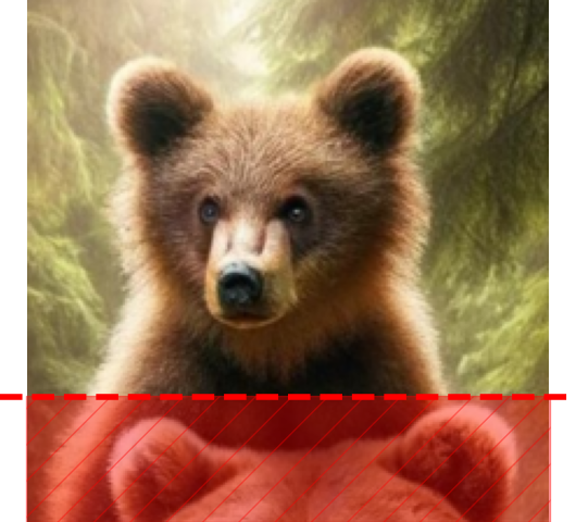
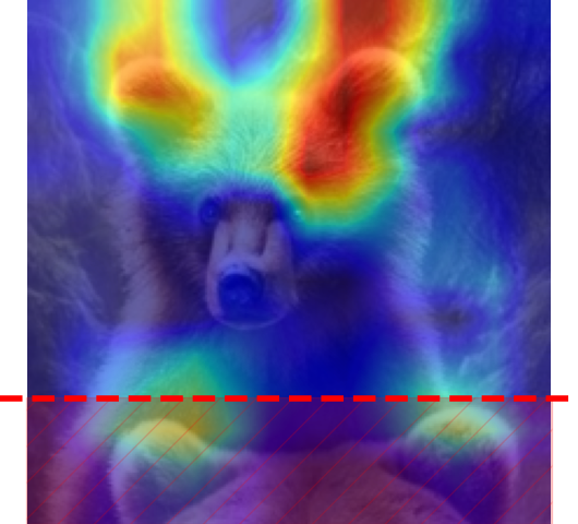
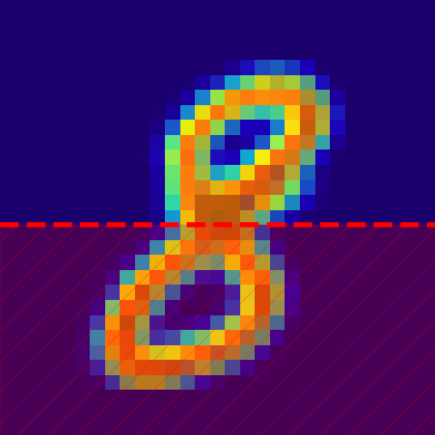
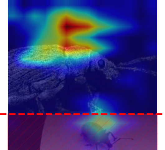
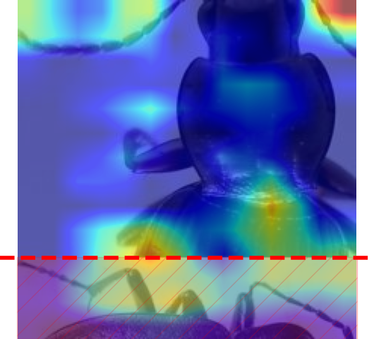
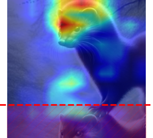
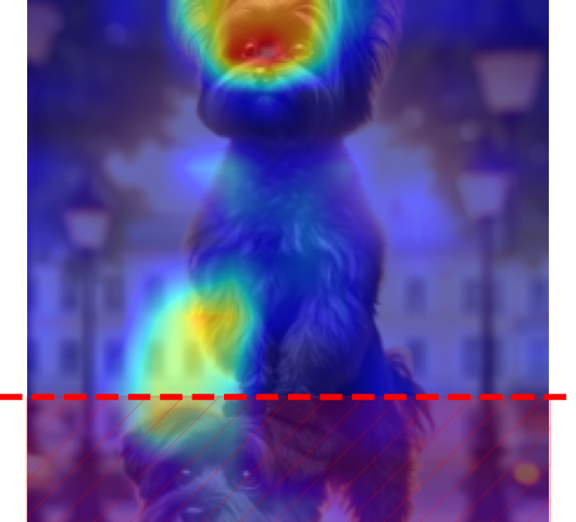
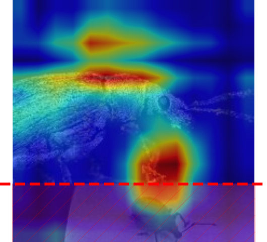
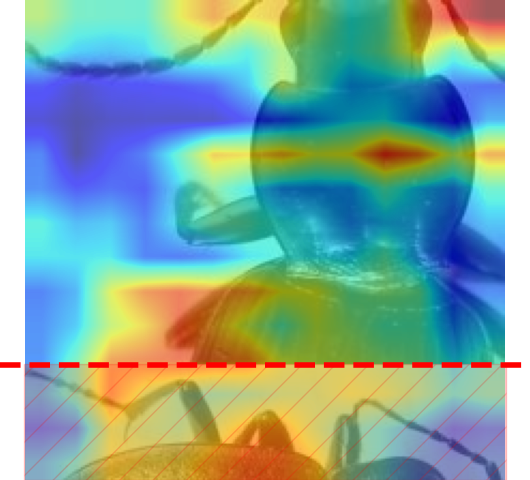
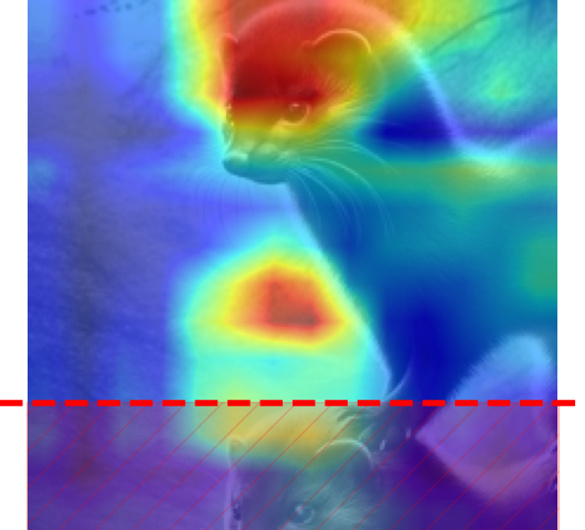
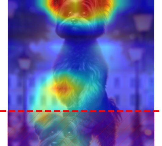
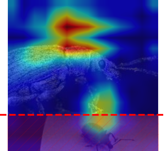
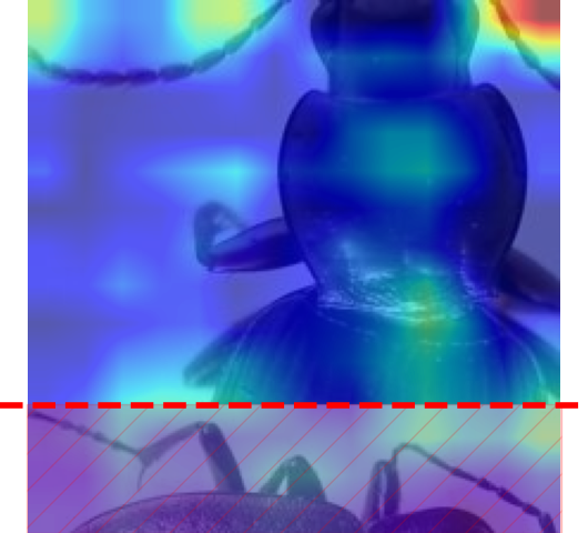
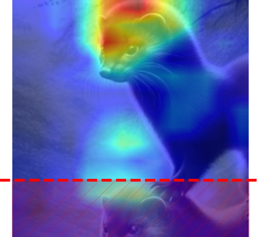
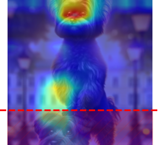
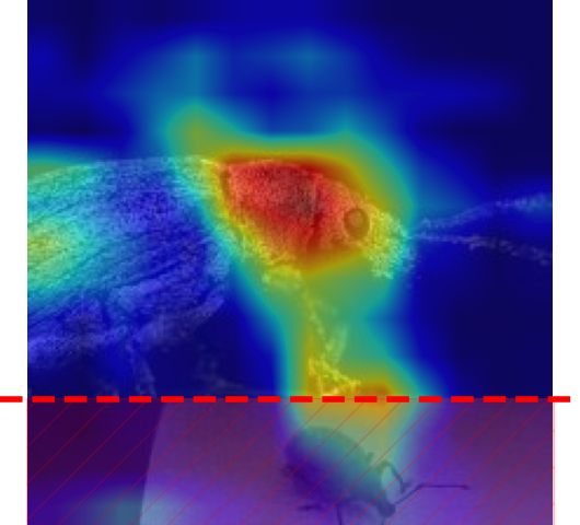
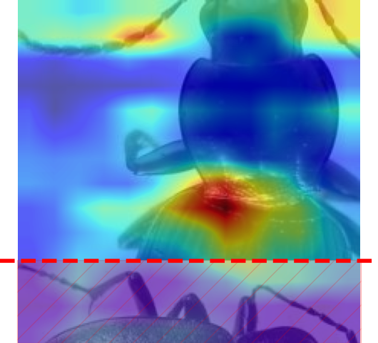
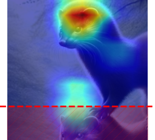
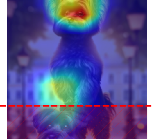
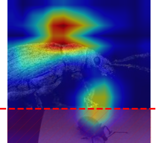
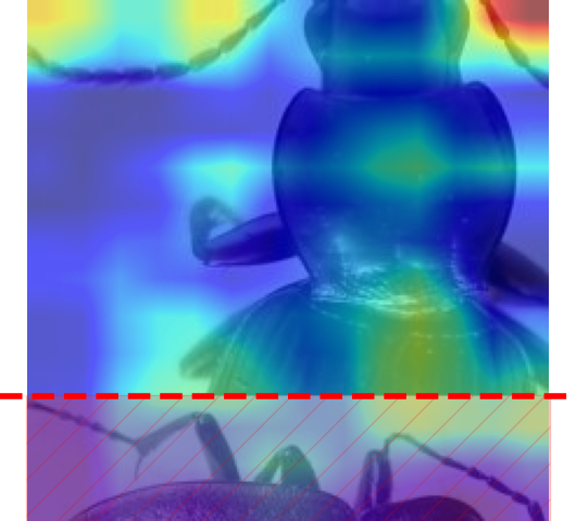
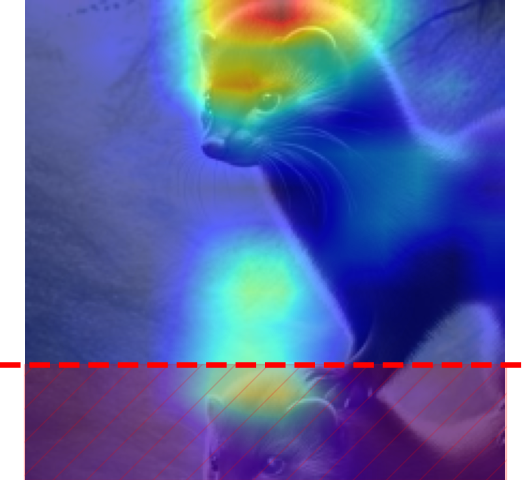
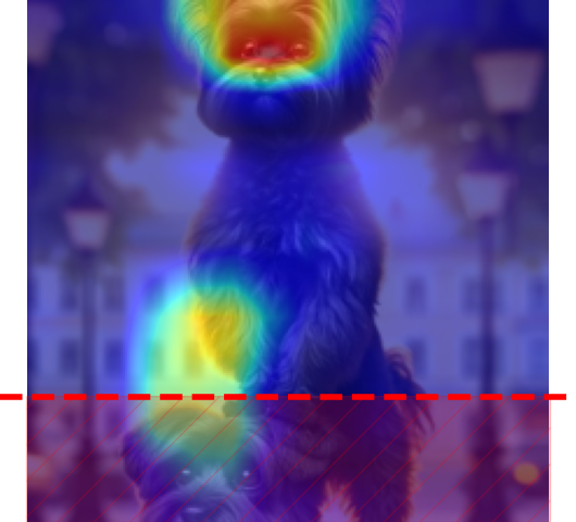
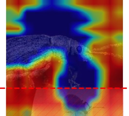
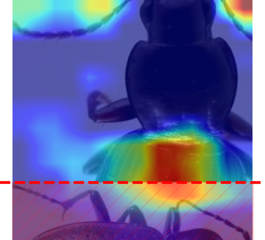
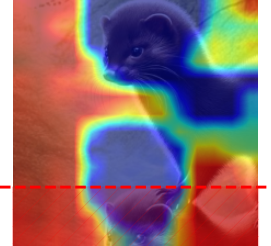
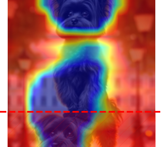
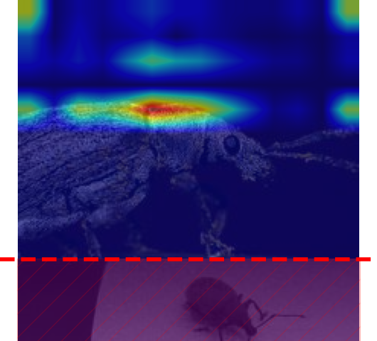
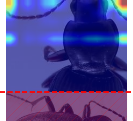
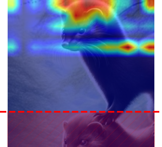
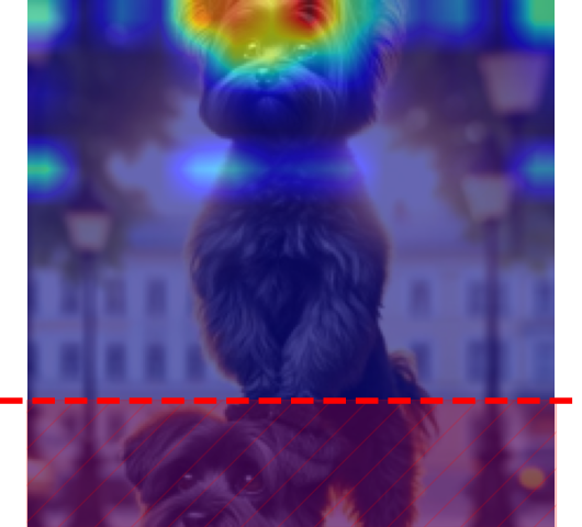
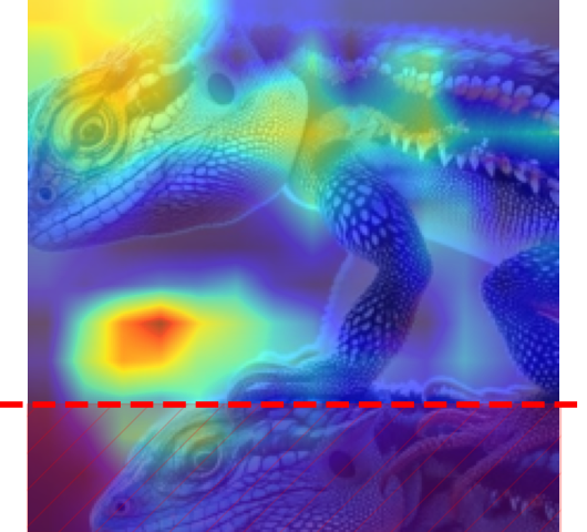
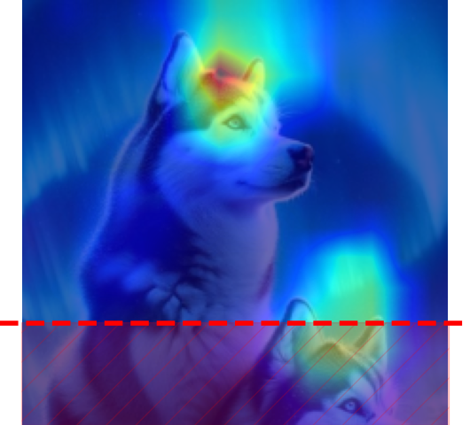
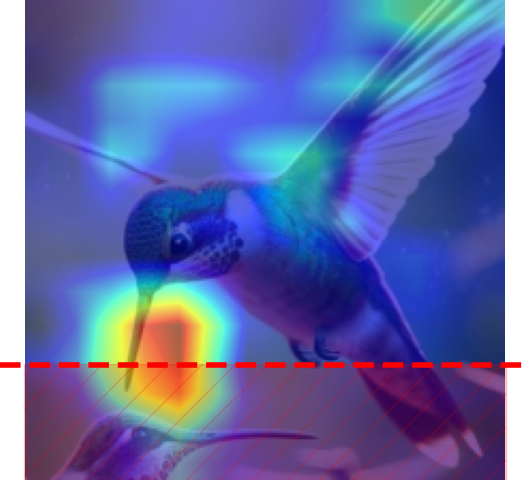
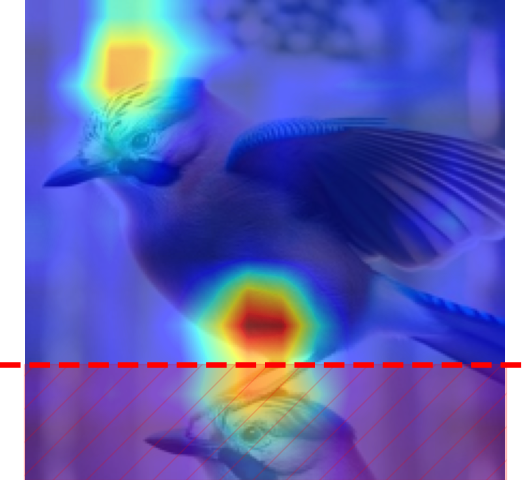
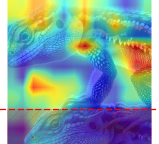
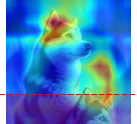
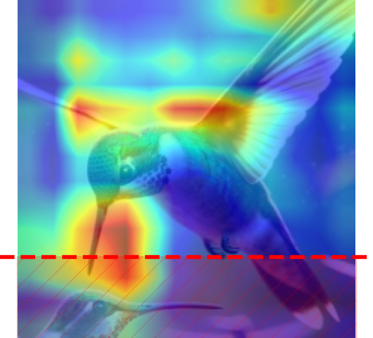
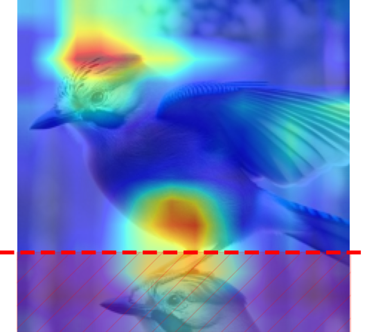
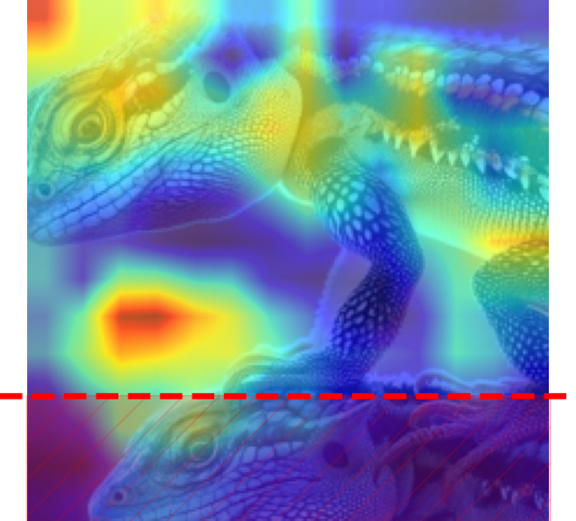
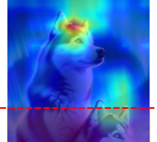
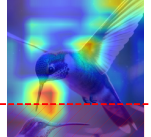
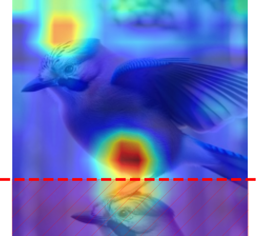
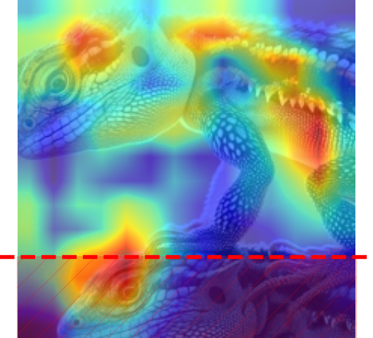
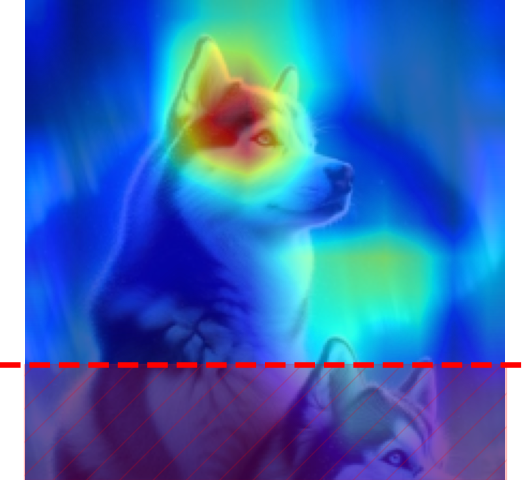
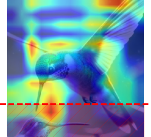
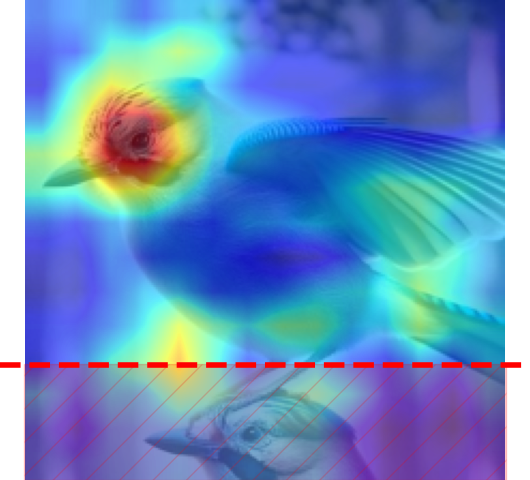
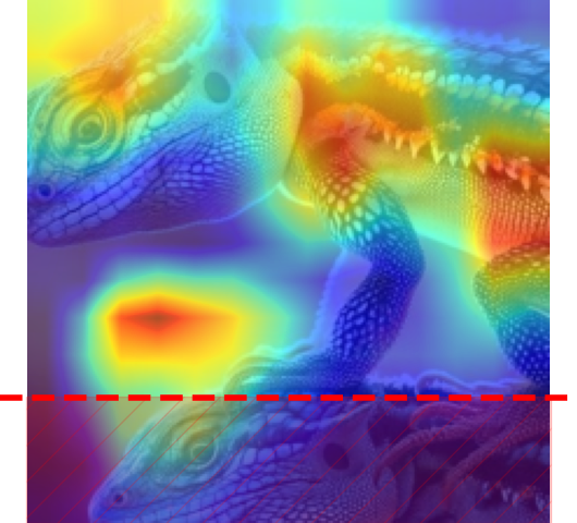
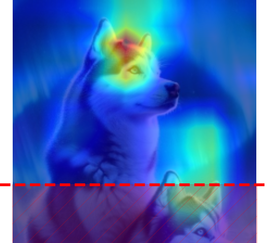
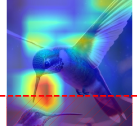
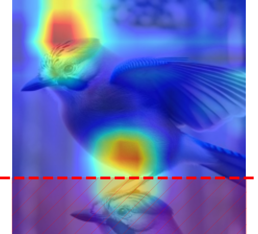
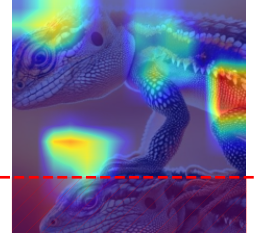
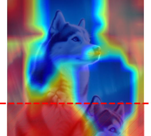
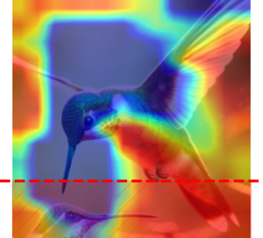
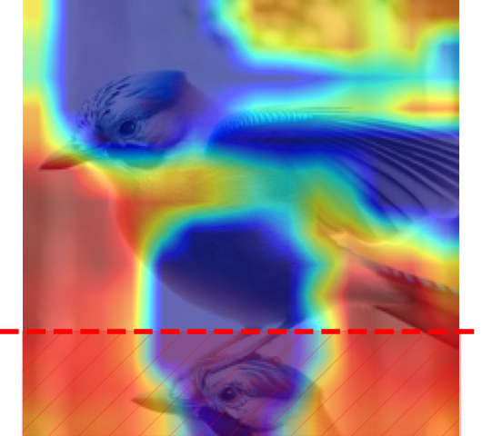
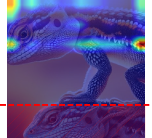
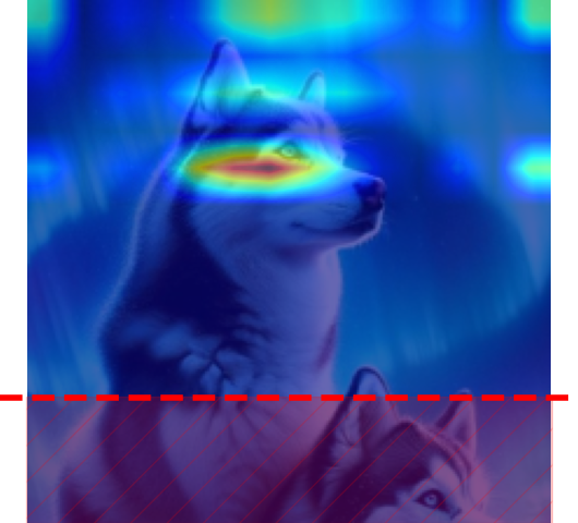
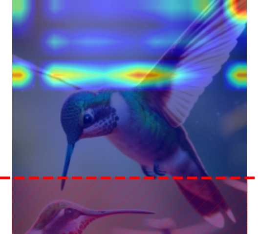
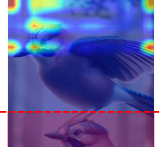
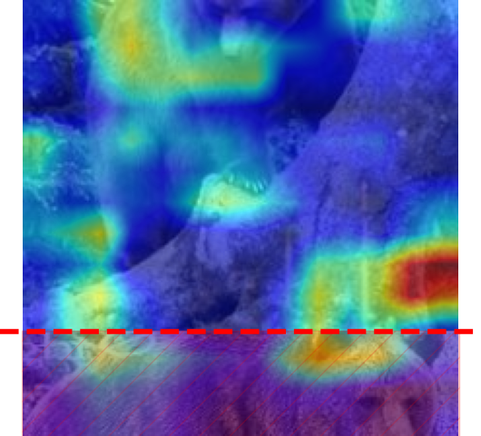
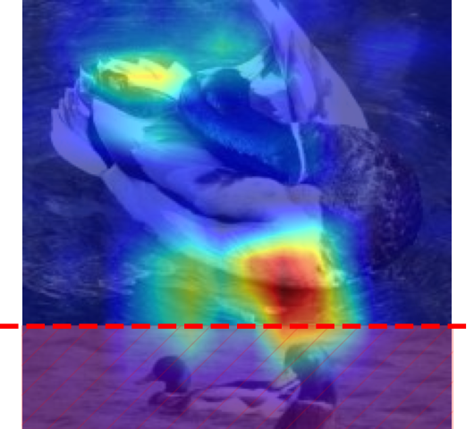
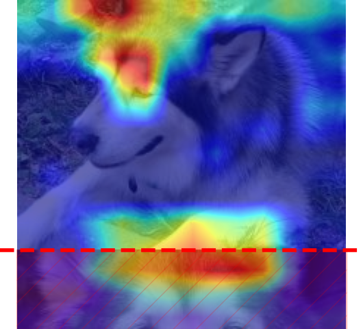
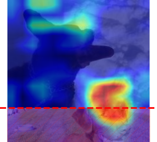
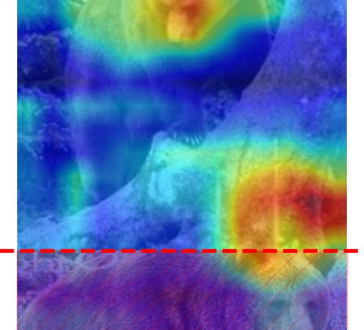
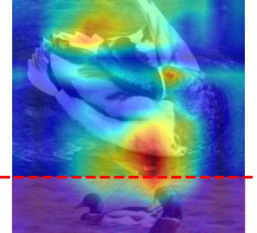
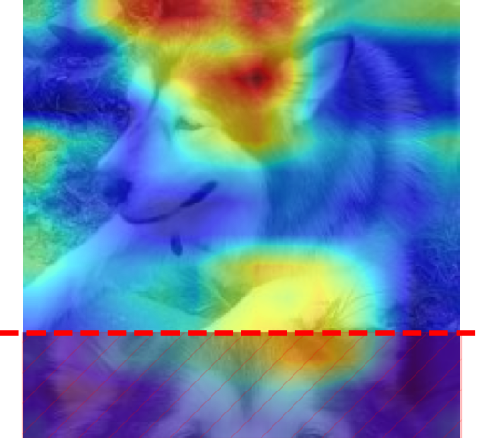
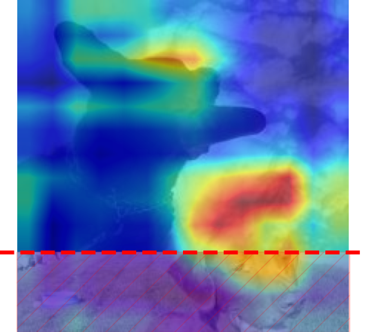
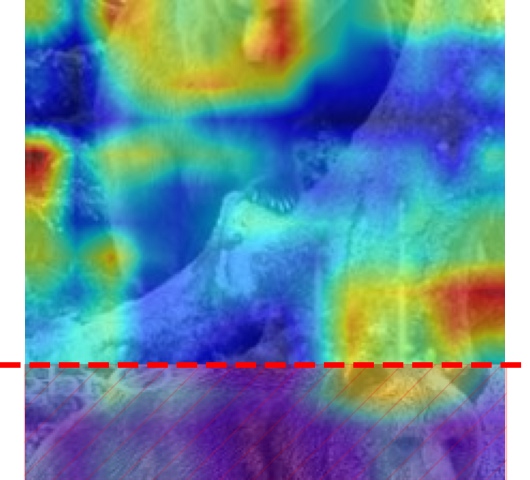
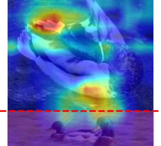
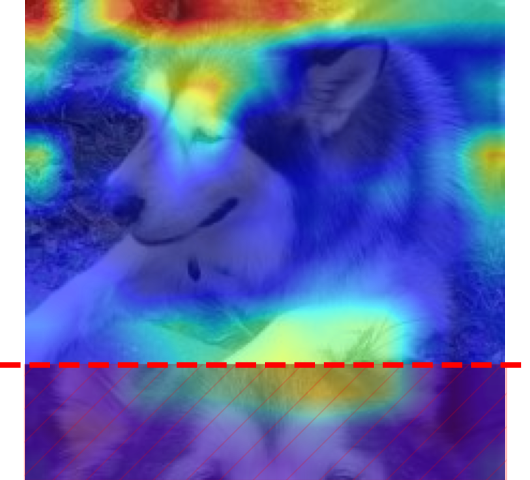
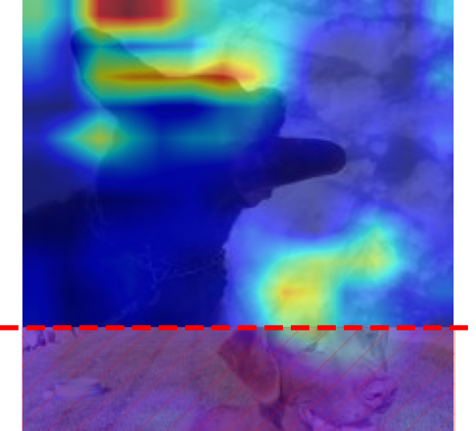
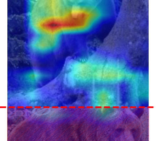
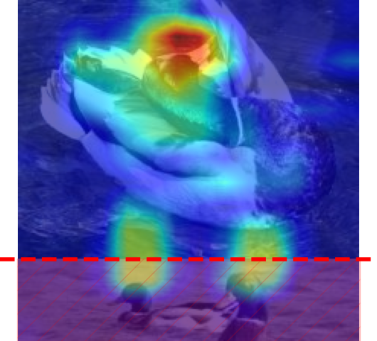
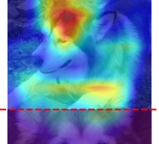
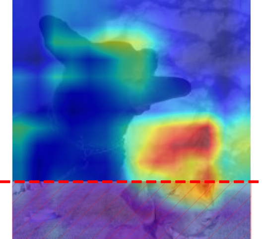
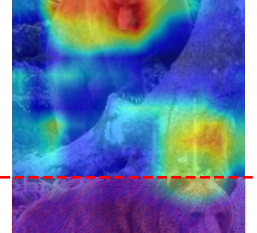
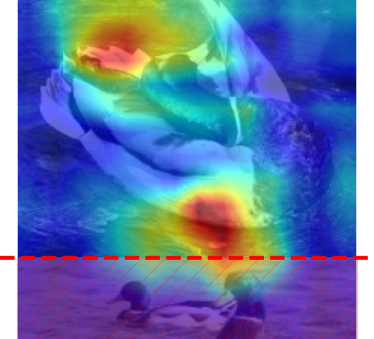
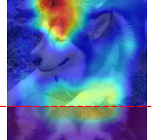
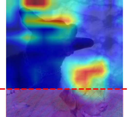
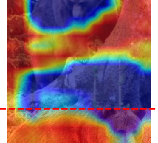
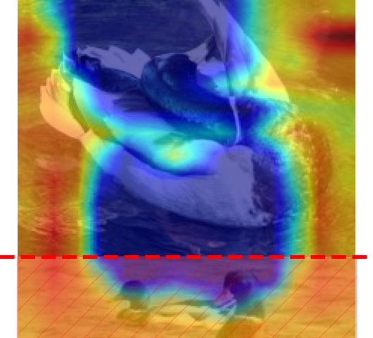
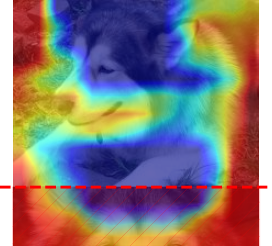
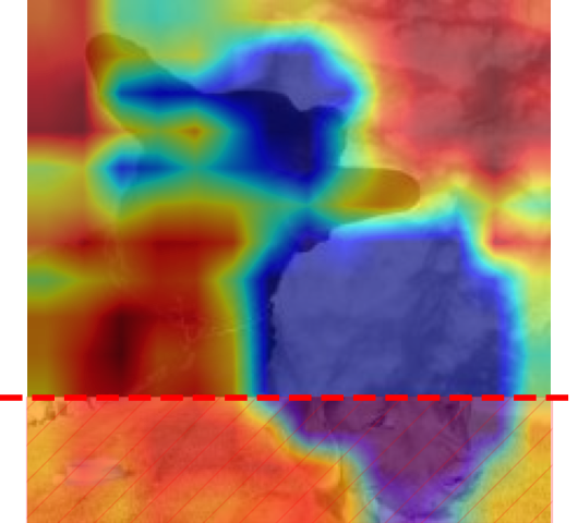
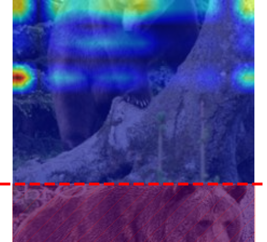
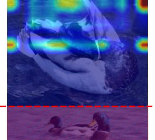
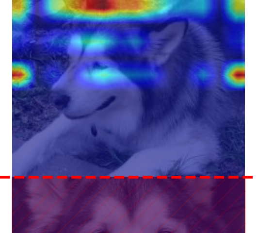
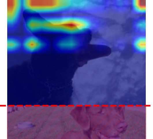
A close inspection of each of these methods reveals that the coefficient associated to each individual map is global, in the sense that the same coefficient is applied to the whole map. The main message of this paper is that this can be problematic, since different parts of the activation map may be used differently by the subsequent layers. Worse, some parts may even be unused by the subsequent network and still highlighted in the final explanation (see Figure 1). Thus we believe that, while giving apparently more-than-satisfying results in practice, CAM-based methods should be used with caution, keeping in mind that some parts of the image may be highlighted whereas they are not even seen by the network.
heightadjust=all, valign=c {floatrow} \ffigbox[\FBwidth]
 \ffigbox[\FBwidth]
 \ffigbox[\FBwidth]
1.1 Related work
This paper is inspired by a line of recent works concerned with the reliability of saliency maps claiming that solely relying on the visual explanation provided by a saliency map can be misleading (Kindermans et al., 2019; Ghorbani et al., 2019). Ghorbani et al. (2019) introduce a method for altering the input data with imperceptible perturbations which do not change the predicted label, yet generating different saliency maps. On the other hand, Kindermans et al. (2019) show that numerous saliency methods generate incorrect scores for the input features when the model prediction is invariant to translation of the input data by a constant. It is important to note that neither of these studies specifically challenges the reliability of CAM-based methods.
This perspective on saliency maps is supported by the work of Adebayo et al. (2018), which introduces a randomization-based sanity check indicating that some existing saliency methods are independent of both the model and the data. We note that GradCAM passes the sanity checks proposed by Adebayo et al. (2018). Draelos and Carin (2021), proposing HiResCAM, are less positive regarding GradCAM pointing out, as we do, that the use of a global coefficient can produce positive explanations where there should not be. Compared to our work, they provide few theoretical explanations and perform experiments on model which are not using parts of the input image.
Taking another angle, Heo et al. (2019) directly attacks the reliability of GradCAM saliency maps by adversarial model manipulation, i.e., fine-tuning a model with the purpose of making GradCAM saliency maps unreliable. This is achieved by using a specific loss function tailored to this effect. Our approach is different, as we simply force a strong form of sparsity in the model’s parameters, not targeting a specific interpretability method.
1.2 Organization of the paper
We start by looking at GradCAM in Section 2. For a given simple CNN architecture described in Section 2.1, we derive closed-form expressions for its explanations in Section 2.2. Leveraging these expressions, we prove in Section 2.3 that GradCAM explanations are positive at initialization, even though a large part of the weights are set to zero.
In Section 3, we demonstrate experimentally that this phenomenon remains true after training. To this extent, we proceed in two steps. First, we train to a reasonable accuracy a VGG-like model on ImageNet (Deng et al., 2009) which does not see the lower part of input images, described in Section 3.1. Then, we create two datasets (Section 3.2) consisting in superposition of images of the same class. We show experimentally in Section 3.3 that CAM-based methods applied to this model wrongly highlights a large portion of the lower part of the images, misleading the user by showing that the lower part is used for the prediction whereas, by construction it is not. The code for all experiments and the datasets are available online.111https://github.com/MagamedT/cam-can-see-through-walls We conclude in Section 4.
2 Mathematical description
The model used for the theoretical analysis done in Section 2.3 is described in Section 2.1, the derivation of GradCAM coefficients in Section 2.2.
2.1 A simple CNN
Let us describe mathematically the model we consider, denoted by and depicted in Figure 2. On a high-level, is a -layers network, consisting in a single convolution / max pooling layer, followed by a -layers fully-connected neural network with ReLU activations. Thus the case corresponds to a single convolutional / max pooling layer followed by a linear transformation.
More precisely, we consider a grayscale image as input. For instance, if we consider the MNIST dataset (LeCun et al., 1998), . We note that our analysis can be easily extended to RBG images. The convolutional layer consists of filters , represented as a collection of matrices of shape .
Formally, the output of the convolution step, , is given by:
| (1) |
where .
In practice, the filter weights are initialized randomly, typically i.i.d. uniform or Gaussian with proper scaling. There are two main trends on how to scale the variance, either Glorot (Glorot and Bengio, 2010) (also called Xavier), or He (He et al., 2015). The later with uniform distribution is default for the CNN layer used in PyTorch. However, we assume from now on i.i.d. Gaussian initialization in our analysis for mathematical convenience.
After the convolution step, we apply a ReLU non-linearity, denoted by . We define the rectified activation maps , where is applied coordinate-wise. Next, we consider a down-sampling layer, here a () max pooling . One can see that the output of the max pooling, , is given by:
| (2) |
where . Note that we assume to divide and for simplicity.
Finally, let us describe recursively the fully-connected part of , denoted by :
| (3) |
where is a weight matrix connecting layer and with and the size of layer . Note that we set , and , since we see the output of our model as the un-normalized logit associated to a given class of a prediction problem. We also, denote by the non-rectified activation of layer and its rectified counterpart.
Summary.
The model we consider can be described concisely as . As explained in introduction, given the nature of CAM-based explanations, it is convenient to split in two functions and for the computations of the next Section 2.2. More precisely, we write
| (4) |
Recall that we refer to Figure 2 for an illustration.
2.2 Closed-form expression
The original idea of CAM (Zhou et al., 2016) was limited to computing the saliency map as a linear combination of the feature maps in the last convolutional layer when . Later, GradCAM (Selvaraju et al., 2017) removed the architecture constraints by computing the average gradient of each feature map with respect to . In our notation, we have:
Definition 1 (GradCAM)
For an input and model , the GradCAM feature scores are given by
where each . Here, GAP denotes the global average pooling, that is, the average of all values, and the ReLU as before.
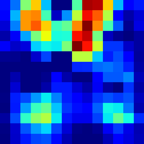
Definition 1 is of course to be taken coordinate-wise. We note that, in practice, is up-sampled and normalized to produce a saliency map with the same shape as the input image. To be more precise, what we define as is the middle panel of Figure 1, whereas the final user will nearly always visualize the right panel. The most important thing to notice in Definition 1 is that is a global coefficient.
We now show why this can be an issue. Looking at Definition 1, whenever the underlying model is not too complicated, one can actually hope to derive a closed-form expression for the feature importance scores of as a function of the model’s parameters. This is achieved by:
Proposition 2 ( coefficients for GradCAM, )
Recall that the vectors denote the non-rectified activation and the weights of the linear part of . Then, for input , the coefficient is given by
where we set and .
From Proposition 2, we immediately deduce a closed-form expression for GradCAM explanations. We note that Proposition 2 can be readily extended to an arbitrary number of filters , in which case the and should be interpreted as corresponding to the relevant .
The proof of Proposition 2 can be found in Appendix C. In Appendix A, we describe mathematically several other CAM-based methods in the setting of : XGradCAM (Fu et al., 2020), GradCAM++ (Chattopadhay et al., 2018), HiResCAM (Draelos and Carin, 2021), ScoreCAM (Wang et al., 2020) and AblationCAM (Desai and Ramaswamy, 2020). A close inspection of these definitions reveals that they also use global weighting coefficients applied to the corresponding activation maps, with the notable exception of HiResCAM.
2.3 Theoretical analysis
Leveraging the results of Section 2.2, we are able to describe precisely the behavior of GradCAM at initialization for , specifically when the classifier part of our model comprises a single layer (). This analysis is justified by existing works (Lee et al., 2019; Du et al., 2019; Allen-Zhu et al., 2019b, a; Zou et al., 2020) showing that neural networks often stay “near initialization” during training. As promised, we conduct this analysis when the network does not have access to the lower part of the image. Our main result is:
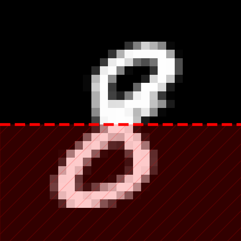
Theorem 3 (Expected GradCAM scores, , masked )
Let be an input image. Let be the patch of corresponding to index . Assume that is even, and . Assume that the filter values and the non-zero weights are initialized i.i.d. . Then, if the number of filters is greater than , we have the following expected lower bound on the GradCAM explanation for pixel :
| (5) |
where the expectation in the previous inequality is taken with respect to initialization of the filters and the remaining weights of the linear layer.
Setting to disables the weights within that are linked to the lower half part of the activation map , effectively preventing from accessing the lower half of . As a consequence, does not see the lower half of , up to side effects. The main consequence of Theorem 3 is that, when the number of filters associated to the class to explain is large enough, is positive in expectation if some pixels are activated in the receptive field associated to . Thus GradCAM highlights all parts of the image where there is some “activity,” even though this information is not used by the network in the end. We illustrate Theorem 3 in Figure 3. The main limitation of this analysis is its focus on the behavior at initialization: we investigate in the following whether this behavior also happens after training. Another limitation is the restriction to a single linear layer, but we note that taking in the fully connected part of is a dominant approach since ResNet (He et al., 2016).
3 Experiments
We know ask the following question: are the consequences of Theorem 3 true after training, and for a more realistic model? To this extent, we train a CNN-based model which by construction cannot access some specified part of the input which we call the dead zone (see Figure 4, details in Section 3.1). Clearly, since the dead zone does not influence the output, it should not contain positive model explanations. To test whether this is true, we create two datasets (Section 3.2). Each item of the first one is composed of two images from ImageNet with the same label in both the seen and the unseen part of the image. The second dataset is built using generative models on the same categories with two objects in each image located in the seen and unseen part as well. We then check whether CAM-based methods wrongly highlight areas in the dead zone in Section 3.3.
3.1 Model
Model definition.
The CNN used in our experiments is a modification of a classical VGG16 architecture (Simonyan and Zisserman, 2015) which we call . Whereas the original VGG16 model is composed of convolutional blocks including either or convolutional layers with ReLU and max pooling, followed by dense layers. In we remove the last max pooling (in the fifth convolutional block) and we further apply a mask on selected neurons of the first dense layer so the layer can not see the lower part of the activation maps, see Figure 4 for more details.
Masking.
We forbid the network from seeing the dead zone in a very simple way: in the first dense layer , which has size , we permanently set to a band of height corresponding to the lower weights. Formally, this means setting , which is denoted in red above in Figure 4. Effectively, we are building a wall that stops all information flowing from the last convolutional layer to the remainder of the network. Since the weights are directly connected to the final activation map , this masking effectively zeroes out the lower sections in each channel denoted by . We can trace back the zeroed activations in to the preceding activation map , pinpointing the exact patches in that correspond (after convolution) to the features observed in the zeroed activation of . Because of the side effects in the computation of convolutions, this area of is slightly smaller: some pixel activation will still play a role in the model’s prediction. Repeating this process until we reach the original image yields a dead zone of height pixels, highlighted in red above in Figure 4, which covers of the image area. As we mentioned earlier, the other main difference with VGG16 is the removing of the final max pooling layer. This leads to a larger activation layer, allowing us to set weights to zero without hindering too much the network’s ability, see Figure 5. We note that bears a strong resemblance to . The main difference is that the convolutional layer of is replaced by several convolutional blocks in , see Figure 4.
Training.
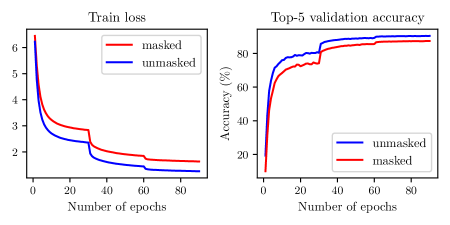
We train on Imagenet-1k (Deng et al., 2009) using classical data augmentation recipe, i.e., random flip and random crop. As optimization algorithm, we use stochastic gradient descent with momentum, weight decay, and a learning rate scheduler. To observe the slight accuracy drop induced by masking a significant part of images, we train a baseline model without masking. We report the train loss and the validation accuracy across training in Figure 5.
Comparison to SOTA.
We also compare the validation top-1 and top-5 accuracy of the VGG16 model found in the PyTorch repository. Our without max pooling and no masking offers the same performance: top-1 and top-5 accuracy on the validation set. As we mention in Figure 5, our model with masking has lower performance, which is expected as a fourth of the input image, , is unseen by the model. We obtain , resp. , top-1 and , resp. , top-5 accuracy on the validation set for our masked , resp. unmasked . Nevertheless, we see that is a realistic network able to predict ImageNet classes with reasonable accuracy. We believe that the drop in accuracy is only minor because ImageNet images are centered, and there is enough information in the upper part of the image to achieve near-perfect prediction.
3.2 Proposed datasets
|
STACK-MIX |
 |
 |
 |
 |
|---|---|---|---|---|
|
STACK-GEN |
 |
 |
 |
 |
Objective.
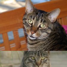
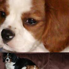
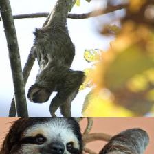
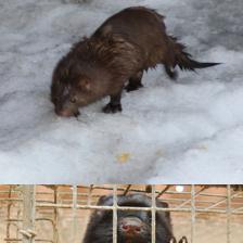
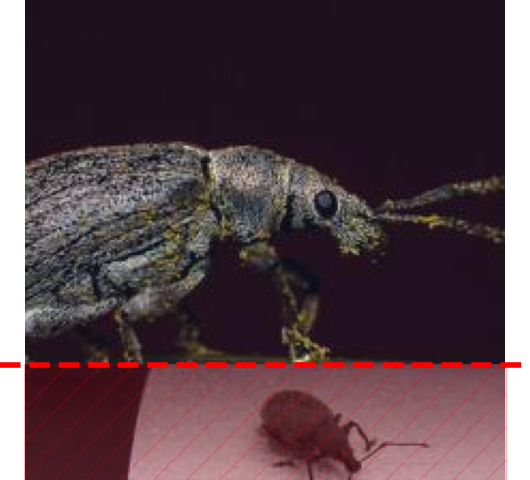
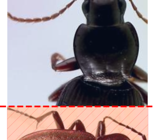
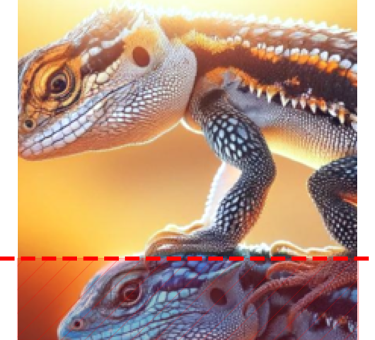
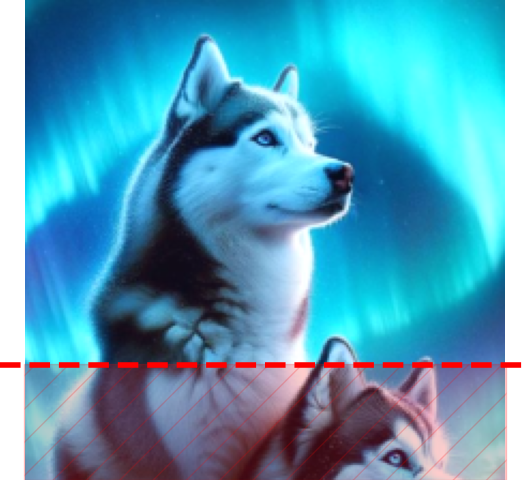
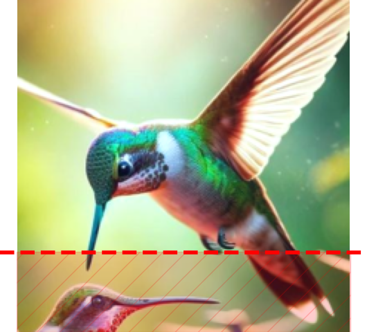
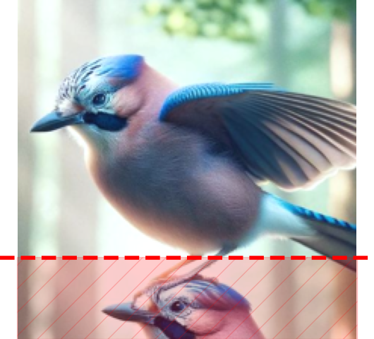
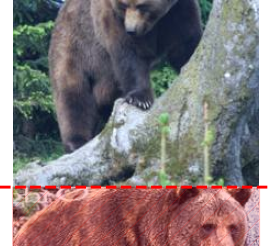
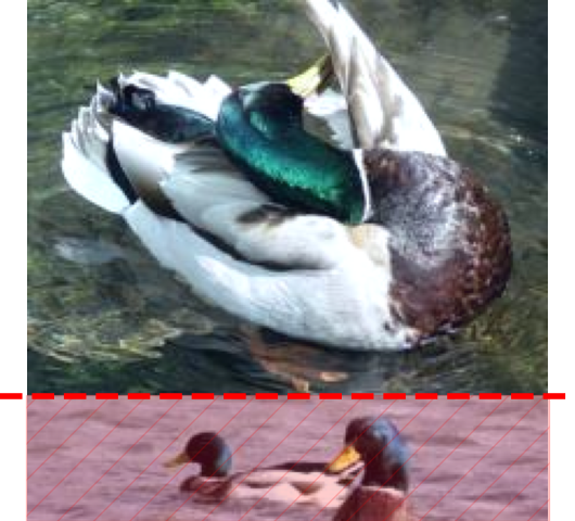
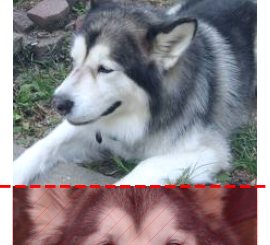
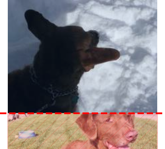
To assess how much CAM-based saliency maps emphasize irrelevant areas of an image, we introduce two new datasets in which we control the positions of the image elements using two techniques: cutmix (Yun et al., 2019) and generative model. More precisely, we produce two datasets, called STACK-MIX and STACK-GEN. Where each image contains two objects, one in the bottom part of the image which is the dead zone for , and the second subject at the top of the image. Therefore, the subject at the center of the image will be mainly responsible for the top-1 predicted score by our masked .
STACK-MIX.
We first generate labels for our datasets by ramdomly sampling classes from the first labels of Imagenet, which corresponds to animals.
The first dataset, called STACK-MIX, consists of images featuring one image from each of the classes. Each example is created by mixing, in a cutmix (Yun et al., 2019) fashion, two images with same label and sampled randomly in the validation set of Imagenet as follows:
| (6) |
meaning that we create a composite image by superposing an upper vertical slice, taken from the top region of with size , with a lower vertical slice, taken from the bottom region of with size . Finally, the quality of the generated images is verified through manual inspection. This dataset lacks realism due to the distinct separation between the two subjects. We address this issue with the help of generative models.
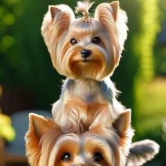
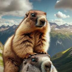
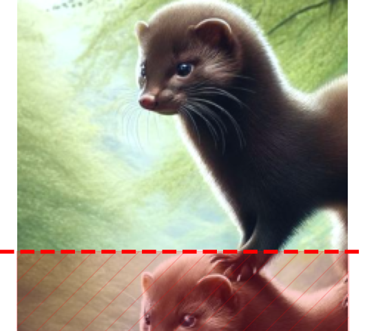
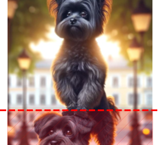
STACK-GEN.
The second dataset, called STACK-GEN, consists of images featuring one image from each of the same classes. It was generated using ChatGPT + DALL·E 3 (Brown et al., 2020; Ramesh et al., 2021) by sampling prompts of the following form: “A photo of {animal name} stacked on top of {same animal name}.” The word “stacked” determines the positions of the subjects in the generated image, which proceeds as follows: first, ChatGPT refines the original prompt to enhance its suitability for DALL·E 3, then the image is generated. We then preprocess the generated images by selectively editing them to minimize the background and centering the focus on the two animals. This editing involves cropping the images to a 1:1 ratio, ensuring one animal is predominantly within the dead zone as defined by our , while the other is positioned in the upper part of the new image. Figure 6 shows examples of the created images. Recall that both datasets are available on the github repository of the project.
|
Input image |
 |
 |
 |
 |
|---|---|---|---|---|
|
GradCAM |
 |
 |
 |
 |
|
GradCAM++ |
 |
 |
 |
 |
|
XGradCAM |
 |
 |
 |
 |
|
ScoreCAM |
 |
 |
 |
 |
|
AblationCAM |
 |
 |
 |
 |
|
EigenCAM |
 |
 |
 |
 |
|
HiResCAM |
 |
 |
 |
 |
3.3 Results
| methods | STACK-MIX | STACK-GEN |
|---|---|---|
| GradCAM (Selvaraju et al., 2017) | ||
| GradCAM++ (Chattopadhay et al., 2018) | ||
| XGradCAM (Fu et al., 2020) | ||
| ScoreCAM (Wang et al., 2020) | ||
| AblationCAM (Desai and Ramaswamy, 2020) | ||
| EigenCAM (Bany Muhammad and Yeasin, 2021) | ||
| HiResCAM (Draelos and Carin, 2021) |
For our , we generate saliency maps from various CAM-based methods on our two datasets, STACK-MIX and STACK-GEN, using the predicted category for each example. Then, we measure how much of the CAM-based saliency maps emphasize the unseen part, i.e., the dead zone. We use the metric defined for a upscaled saliency map as follows:
| (7) |
where is the -norm and the lower part of the image is unseen by our . We note that for a saliency map , the lower , the better.
4 Conclusion
In this paper, we looked into several CAM-based methods, with a particular focus on GradCAM. We showed that they can highlight parts of the input image that are provably not used by the network. This was also showed theoretically, looking at the behavior of GradCAM for a simple, masked CNN at initialization: the saliency map is positive in expectation, even in areas which are unseen by the network. Experimentally, this phenomenon appears to remain true, even on a realistic network trained to a good accuracy on ImageNet.
As future work, we would like to extend the theory to a ResNet-like architecture and other CAM-based methods, such as LayerCAM (Jiang et al., 2021). We also would like to multiply the number of images in our two new datasets, with the hope that this framework can become a standard check for saliency maps explanations.
Acknowledgements
This work was funded in part by the French Agence Nationale de la Recherche (grant number ANR-19-CE23-0009-01 and ANR-21-CE23-0005-01). Most of this work was realized while DG was employed at Université Côte d’Azur. We thank Jenny Benois-Pineau for her valuable insights.
References
- Adebayo et al. (2018) Julius Adebayo, Justin Gilmer, Michael Muelly, Ian Goodfellow, Moritz Hardt, and Been Kim. Sanity checks for saliency maps. In Advances in Neural Information Processing Systems, volume 31, 2018.
- Allen-Zhu et al. (2019a) Zeyuan Allen-Zhu, Yuanzhi Li, and Zhao Song. On the convergence rate of training recurrent neural networks. Advances in Neural Information Processing Systems, 32, 2019a.
- Allen-Zhu et al. (2019b) Zeyuan Allen-Zhu, Yuanzhi Li, and Zhao Song. A Convergence Theory for Deep Learning via Over-Parameterization. In Proceedings of the 36th International Conference on Machine Learning, 2019b.
- Bany Muhammad and Yeasin (2021) Mohammed Bany Muhammad and Mohammed Yeasin. Eigen-CAM: Visual Explanations for Deep Convolutional Neural Networks. SN Computer Science, 2(1):47, 2021.
- Beauchamp (2018) Maxime Beauchamp. On numerical computation for the distribution of the convolution of N independent rectified Gaussian variables. Journal de la Société Française de Statistique, 2018.
- Benítez et al. (1997) José Manuel Benítez, Juan Luis Castro, and Ignacio Requena. Are artificial neural networks black boxes? IEEE Transactions on Neural Networks, 8(5):1156–1164, 1997.
- Brown et al. (2020) Tom Brown, Benjamin Mann, Nick Ryder, Melanie Subbiah, Jared D Kaplan, Prafulla Dhariwal, Arvind Neelakantan, Pranav Shyam, Girish Sastry, Amanda Askell, et al. Language models are few-shot learners. Advances in Neural Information Processing Systems, 2020.
- Chattopadhay et al. (2018) Aditya Chattopadhay, Anirban Sarkar, Prantik Howlader, and Vineeth N Balasubramanian. Grad-CAM++: Generalized Gradient-Based Visual Explanations for Deep Convolutional Networks. In IEEE Winter Conference on Applications of Computer Vision, pages 839–847, 2018.
- Deng et al. (2009) Jia Deng, Wei Dong, Richard Socher, Li-Jia Li, Kai Li, and Li Fei-Fei. ImageNet: A large-scale hierarchical image database. In IEEE Conference on Computer Vision and Pattern Recognition, pages 248–255, 2009.
- Desai and Ramaswamy (2020) Saurabh Desai and Harish G. Ramaswamy. Ablation-CAM: Visual Explanations for Deep Convolutional Network via Gradient-free Localization. In IEEE Winter Conference on Applications of Computer Vision (WACV), pages 972–980, 2020.
- Draelos and Carin (2021) Rachel Lea Draelos and Lawrence Carin. Use HiResCAM instead of Grad-CAM for faithful explanations of convolutional neural networks. arxiv preprint 2011.08891, 2021.
- Du et al. (2019) Simon Du, Jason Lee, Haochuan Li, Liwei Wang, and Xiyu Zhai. Gradient descent finds global minima of deep neural networks. In Proceedings of the 36th International Conference on Machine Learning, 2019.
- Fu et al. (2020) Ruigang Fu, Qingyong Hu, Xiaohu Dong, Yulan Guo, Yinghui Gao, and Biao Li. Axiom-based Grad-CAM: Towards Accurate Visualization and Explanation of CNNs. In 31st British Machine Vision Conference, 2020.
- Fukushima (1980) Kunihiko Fukushima. Neocognitron: A self-organizing neural network model for a mechanism of pattern recognition unaffected by shift in position. Biological Cybernetics, 36(4):193–202, 1980.
- Ghorbani et al. (2019) Amirata Ghorbani, Abubakar Abid, and James Zou. Interpretation of neural networks is fragile. In Proceedings of the AAAI Conference on Artificial Intelligence, 2019.
- Glorot and Bengio (2010) Xavier Glorot and Yoshua Bengio. Understanding the difficulty of training deep feedforward neural networks. In Proceedings of the 13th International Conference on Artificial Intelligence and Statistics, pages 249–256, 2010.
- He et al. (2015) Kaiming He, Xiangyu Zhang, Shaoqing Ren, and Jian Sun. Delving deep into rectifiers: Surpassing human-level performance on imagenet classification. In Proceedings of the IEEE International Conference on Computer Vision, pages 1026–1034, 2015.
- He et al. (2016) Kaiming He, Xiangyu Zhang, Shaoqing Ren, and Jian Sun. Deep residual learning for image recognition. In Proceedings of the IEEE Conference on Computer Vision and Pattern Recognition, pages 770–778, 2016.
- Heo et al. (2019) Juyeon Heo, Sunghwan Joo, and Taesup Moon. Fooling Neural Network Interpretations via Adversarial Model Manipulation. In Advances in Neural Information Processing Systems, volume 32, 2019.
- Jiang et al. (2021) Peng-Tao Jiang, Chang-Bin Zhang, Qibin Hou, Ming-Ming Cheng, and Yunchao Wei. Layercam: Exploring hierarchical class activation maps for localization. IEEE Transactions on Image Processing, 2021.
- Kindermans et al. (2019) Pieter-Jan Kindermans, Sara Hooker, Julius Adebayo, Maximilian Alber, Kristof T Schütt, Sven Dähne, Dumitru Erhan, and Been Kim. The (un) reliability of saliency methods. Explainable AI: Interpreting, explaining and visualizing deep learning, 2019.
- LeCun et al. (1998) Yann LeCun, Léon Bottou, Yoshua Bengio, and Patrick Haffner. Gradient-based learning applied to document recognition. Proceedings of the IEEE, 86(11):2278–2324, 1998.
- Lee et al. (2019) Jaehoon Lee, Lechao Xiao, Samuel Schoenholz, Yasaman Bahri, Roman Novak, Jascha Sohl-Dickstein, and Jeffrey Pennington. Wide neural networks of any depth evolve as linear models under gradient descent. Advances in Neural Information Processing Systems, 32, 2019.
- Linardatos et al. (2021) Pantelis Linardatos, Vasilis Papastefanopoulos, and Sotiris Kotsiantis. Explainable AI: A Review of Machine Learning Interpretability Methods. Entropy, 23(1):18, 2021.
- Lipton (2018) Zachary C. Lipton. The Mythos of Model Interpretability: In Machine Learning, the Concept of Interpretability is Both Important and Slippery. 2018.
- Ramesh et al. (2021) Aditya Ramesh, Mikhail Pavlov, Gabriel Goh, Scott Gray, Chelsea Voss, Alec Radford, Mark Chen, and Ilya Sutskever. Zero-shot text-to-image generation. In International Conference on Machine Learning, 2021.
- Selvaraju et al. (2017) Ramprasaath R. Selvaraju, Michael Cogswell, Abhishek Das, Ramakrishna Vedantam, Devi Parikh, and Dhruv Batra. Grad-CAM: Visual Explanations from Deep Networks via Gradient-Based Localization. In 2017 IEEE International Conference on Computer Vision (ICCV), pages 618–626, 2017.
- Simonyan and Zisserman (2015) Karen Simonyan and Andrew Zisserman. Very deep convolutional networks for large-scale image recognition. In ICLR, 2015.
- Simonyan et al. (2013) Karen Simonyan, Andrea Vedaldi, and Andrew Zisserman. Deep inside convolutional networks: Visualising image classification models and saliency maps. arXiv preprint arXiv:1312.6034, 2013.
- Wang et al. (2020) H. Wang, Z. Wang, M. Du, F. Yang, Z. Zhang, S. Ding, P. Mardziel, and X. Hu. Score-CAM: Score-Weighted Visual Explanations for Convolutional Neural Networks. In 2020 IEEE/CVF Conference on Computer Vision and Pattern Recognition Workshops, pages 111–119, 2020.
- Yun et al. (2019) S. Yun, D. Han, S. Chun, S. Oh, Y. Yoo, and J. Choe. CutMix: Regularization Strategy to Train Strong Classifiers With Localizable Features. In IEEE/CVF International Conference on Computer Vision, pages 6022–6031, 2019.
- Zhang et al. (2023) Hanwei Zhang, Felipe Torres, Ronan Sicre, Yannis Avrithis, and Stephane Ayache. Opti-CAM: Optimizing saliency maps for interpretability. arXiv preprint arXiv:2301.07002, 2023.
- Zhang et al. (2021) Yu Zhang, Peter Tiňo, Aleš Leonardis, and Ke Tang. A survey on neural network interpretability. IEEE Transactions on Emerging Topics in Computational Intelligence, 2021.
- Zhou et al. (2016) Bolei Zhou, Aditya Khosla, Agata Lapedriza, Aude Oliva, and Antonio Torralba. Learning deep features for discriminative localization. In Proceedings of the IEEE Conference on Computer Vision and Pattern Recognition, pages 2921–2929, 2016.
- Zou et al. (2020) Difan Zou, Yuan Cao, Dongruo Zhou, and Quanquan Gu. Gradient descent optimizes over-parameterized deep relu networks. Machine Learning, 2020.
Appendix A Other definitions
The work of Fu et al. (2020) proposed an alternative to by re-scaling the gradient in the weighting coefficient . The main objective of this alternative is to obtain a method that satisfies two axioms (sensitivity and conservation properties) defined by Fu et al. (2020), which, according to their findings, enhances visualization performance w.r.t. specific metrics.
Definition 4 (XGradCAM)
In our notation, for an input and model , the XGradCAM feature scores are given by
where each is the global average pooling of the gradient of at rescaled by the normalized activation .
GradCAM++ (Chattopadhay et al., 2018) then modified GradCAM by computing rectified gradient together with second and third order derivative information. This alternative appears to produce better saliency maps in cases where the input image contains multiple subjects.
Definition 5 (GradCAM++)
In our notation, for an input and model , the GradCAM++ feature scores are given by
where each is the global average pooling of the gradient of at rescaled by second and third order derivatives defined as
More recently, HiResCAM (Draelos and Carin, 2021) proposed to replace the averaging of the gradient over the map by the element-wise multiplication between gradient and activation. In our notation:
Definition 6 (HiResCAM)
For an input and model , the HiResCAM feature scores are given by
where and is the element-wise matrix product.
The work of Wang et al. (2020) got rid of the dependency on gradients of the weighting coefficients .
Definition 7 (ScoreCAM)
In our notation, for an input and model , the ScoreCAM feature scores are given by
In the previous display, , where , the upsampled and normalized activation map , a normalization function that maps matrix values into , and an upsampling function which resize a matrix to the size of .
Finally, AblationCAM (Desai and Ramaswamy, 2020) removes each activation to observe the impact on the prediction. Ablations resulting in larger drops receive higher weights. AblationCAM is similar to ScoreCAM: a sort of masking is performed to observe changes in prediction and no gradient is required. However, both methods require lots of forward passes through the network.
Definition 8 (AblationCAM)
In our notation, for an input and model , the AblationCAM feature scores are given by
where each , the predicted score by our model and is the output of when the activation map is zero out.
Appendix B Technical results
As a consequence of Eq. (1), (seens as a vector of size ) is a centered Gaussian vector, with covariance matrix given by
| (8) |
Because of this simple remark, we can describe precisely the distribution of (and, further, ), thanks to the following lemmas. We denote by the density of the standard Gaussian distribution and its cumulative distribution function.
Lemma 9 (Expectation of rectified Gaussian)
Let , we get the following expectation for the rectified Gaussian :
Proof
See Beauchamp (2018).
Lemma 10 (Law of convolution)
Let and , then the convolution has distribution .
Proof First let us remind that:
This lemma is derived from rapid calculations that proceed as follows, utilizing the fact that the elements are independent and identically distributed (i.i.d.):
Straightforward computations yields:
Lemma 11 (Moments of squared rectified Gaussian)
Let of density , we get the following two moments for the squared rectified Gaussian :
Appendix C Proof of Proposition 2
Notation.
Before starting the proof, let us recall some notation. In Section 2.1, we defined the non-rectified activation of layer , its rectified counterpart. We also defined the max pooled rectified activation . In this proof, we write the function that maps the input of the -th layer to its output as follows with .
Now let us turn to the computation of with . By the chain rule, we get where:
We compute as follows:
Now let us remark that, for all , , since is applied element-wise. Thus
Finally,
Now to compute let us start from the end with :
Similarly,
so the next computation gives
Now we can conclude by straightforward induction:
Now to finish we need to compute , to do so, we suppose that the convolutional layer returns an reshaped rectified activation map such that we get the following gradient:
with being the -th block of indicator functions defined as follows:
where and is the -th patch of (the patch are ordered from left to right, starting from the top of ). Also note that is the integer division.
Finally, we can compute as follows:
where , is defined as follows:
To compute , we simply take the average of the components of the previous display, , which yields
since with fixed (it is also the case in practice when using automatic differentiation) and .
Appendix D Proof of Theorem 3
Before jumping into the proof, let us remark that the left-hand side of Eq. (5) is non-negative, thus there is nothing to prove if . Thus we will assume that from now on.
Separating the randomness.
There are two sources of randomness: the weights of the filters and the coefficients of the linear layer . We start this proof by dissociating these two sources of randomness. More precisely, following Definition 1, and using the law of total expectation, we compute the expected GradCAM heatmap at coordinates as
| (9) |
Using the computed GradCAM coefficient in Proposition 2 with , we get . Since we assume that the weights of the linear layer are i.i.d. , for the upper part, and for the lower part, is a centered Gaussian with variance . Now, we recall that does not depend on . Therefore, conditionally to , is a centered Gaussian with variance
We deduce that
| (10) |
Computing expectations.
Lower bound.
Up to the best of our knowledge, there is no closed-form expression for Eq. (11), and we now proceed to find a lower bound to this expression. Let . By Lemma 10 and 11, and with a patch at index in the image . By Chebyshev’s inequality, for any ,
| (12) |
Let us set in the previous display, in this way
Since ,
We now conclude the proof writing
Appendix E Additional Experiments
In this section, we present two additional sets of experiments, one on STACK-MIX (Figure 8), the other on STACK-GEN (Figure 9).
|
Input image |
 |
 |
 |
 |
|---|---|---|---|---|
|
GradCAM |
 |
 |
 |
 |
|
GradCAM++ |
 |
 |
 |
 |
|
XGradCAM |
 |
 |
 |
 |
|
ScoreCAM |
 |
 |
 |
 |
|
AblationCAM |
 |
 |
 |
 |
|
EigenCAM |
 |
 |
 |
 |
|
HiResCAM |
 |
 |
 |
 |
|
Input image |
 |
 |
 |
 |
|---|---|---|---|---|
|
GradCAM |
 |
 |
 |
 |
|
GradCAM++ |
 |
 |
 |
 |
|
XGradCAM |
 |
 |
 |
 |
|
ScoreCAM |
 |
 |
 |
 |
|
AblationCAM |
 |
 |
 |
 |
|
EigenCAM |
 |
 |
 |
 |
|
HiResCAM |
 |
 |
 |
 |