Quantifying Noise of Dynamic Vision Sensor

Abstract

Dynamic visual sensors (DVS) are characterized by a large amount of background activity (BA) noise, which it is mixed with the original (cleaned) sensor signal. The dynamic nature of the signal and the absence in practical application of the ground truth, it clearly makes difficult to distinguish between noise and the cleaned sensor signals using standard image processing techniques. In this letter, a new technique is presented to characterise BA noise derived from the Detrended Fluctuation Analysis (DFA). The proposed technique can be used to address an existing DVS issues, which is how to quantitatively characterised noise and signal without ground truth, and how to derive an optimal denoising filter parameters. The solution of the latter problem is demonstrated for the popular real moving-car dataset.

11(2.5, 0.4)

This work has been submitted to the IEEE Signal Processing Letters. Copyright may be transferred without notice, after which this version may no longer be accessible. ©IEEE

I Introduction

Dynamic vision sensor (DVS), also known as silicon retina, is a microelectronic chip for events camera detecting changes in brightness or intensity on a per-pixel basis and storing these changes asynchronously as events [1]. One of the major issues with this type of sensors, is the fact that large amount of background activity (BA) noise can be present in the clean signal, which it may limit the usage of the signal in practical applications. Properly setting of the sensor may partially solve the issue by means of improving the cleanness of the received events stream and this has been demonstrated in various previous works [2], [3], [4], [5], [6]. However, large areas of the signal may still be affected by the BA noise, due to the difficulties to recognise and remove noise induced by the background activity (BA) of the DVS matrix.

A key principle to distinguish BA noise from a signal has been firstly introduced by Delbruck [7],[8]. It is based on the observation that a random noise event is spatially and temporally isolated. The noise is identified by checking eight neighboring pixels and using a single $\Delta T$ parameter for the time interval between the checked event and its correlated events. Also a variety of modifications of the original approach have been presented [9]: (1) accelerate search of neighboring pixels in the vicinity of the central event without change of the original principle (k-noise [10] and DWF [11] filters); (2) introduce additional parameters $\Delta S_{x},\Delta S_{y}$ to expand the allowed space vicinity as well as the minimal number of captured events $\rho_{\text{min}}$ in a 3D $xyt$ box as a threshold (y-noise filter [12]); (3) make projections of the events, which are captured in the 3D box $\Delta S_{x},\Delta S_{y},\Delta T$ onto central plane of the box with various weights (TS [13], IETS [14], MLPF [11] filter). Also, deep-learning based approaches have been presented: PUGM [15], EDnCNN [16], AEDNet [17], and partly MLPF [11].

It is commonly known that it is hard to assess quality of denoised DVS data for two reasons. First, the evaluation may be influenced by the so called accumulation time, i.e., too small only few events are captured, too big the clean signal may result blurred and so it will be identified as noise. Second, any BA filter has tuning parameters, and they need to be carefully selected and based on the adopted accumulation time same parameters values may provide different results.

To avoid an evaluation based mainly on subjective taste, one needs an objective criterion. We may have two approaches, using a ground truth or using image recognition applications performances to evaluate the quality of the noise filtering output. The former approach is available only for synthetic datasets with an artificial noise injected [11], and the latter one exploits a concept of warped events [18], where one needs (a) to perform a clustering of events streams, (b) to determine a optical flow for each cluster by means of optimisation of a contrast maximization goal function, and (c) to use the results of the optimisation to compare different denoising approaches. Obviously, the latter is much more complex. To this scope TS [13] and IETS [14] filters were proposed.

Attempts to label each event as noise or signal have been proposed[16], [17], however, due to the heavy data load of DVS it is completely impractical approach [19].

The above motivations are clearly showing how traditional approaches are limiting themselves in working with each event by checking if it is noise or signal. In this letter we introduce a novel objective criterion, to evaluate noise filtering performances, where a single parameter is derived from the statistical properties of the DVS time series. We quantify filtered DVS noise with detrended fluctuation analysis (DFA). After a brief introduction of the DFA principles, we are showing how DFA might be adapted for DVS data, and then demonstrating its efficiency by separating noise from the cleaned signal. This is shown by testing it on a popular moving-car dataset to find optimal filter characteristics. To our best knowledge, this is the first attempt to use DFA approach to DVS data.

II Dynamic Visual Sensor (DVS)

Dynamic Visual Sensor (DVS) [1] is a 2D matrix of asynchronously pixels. Each pixel has static and dynamic variables. The static one is for previous reference illumination of the pixel and the dynamic one is for the instantaneous illumination. At every tact, the instantaneous and reference illuminations are compared. If their difference is more than a threshold, the pixel updates its reference and triggers an event $e=e(t,x,y,p)$, being $t$ an instance of time, when the event is triggered, $(x,y)$ pixel’s 2D coordinates, and $p=\pm 1$ is polarity of the triggered event (positive, if illumination increases, and negative otherwise). As a result, DVS data is a stream of events $\{e_{1},e_{2},\dots,e_{N}\}$.

III Background Activity (BA) filter

A simple BA filter works as follows [7], [8], [10], [20], [11]. Let $\sigma_{ij}$ be a Boolean variable for a correlation between $e_{i}$ and $e_{j}$ events in the 3D box $(\Delta S_{x},\Delta S_{y},\Delta T)$:

$$\sigma_{ij} =|x_{i}-x_{j}|\leq\Delta S_{x}$$

$$\land|y_{i}-y_{j}|\leq\Delta S_{y}\land|t_{i}-t_{j}|\leq\Delta T.$$ (1)

When $e_{j}$ is vicinity of $e_{i}$, then $\sigma_{ij}$ is true. With $\llbracket\cdot\rrbracket$ as Iverson bracket ($\llbracket\text{true}\rrbracket=1$,$\llbracket\text{false}\rrbracket=0$), the total number of correlated events $\rho_{i}$ in $e_{i}$’s vicinity is given by

$$\rho_{i}(\Delta S_{x},\Delta S_{y},\Delta T) =\sum_{j\neq i}\llbracket\sigma_{ij}\rrbracket,$$ (2)

Then

$$e_{i}(t_{i}x_{i},y_{i},p_{i})= \begin{cases}\text{signal},\text{ if }\rho_{i}\geq\rho_{\text{min}},\\ \text{noise, otherwise.}\end{cases}$$ (3)

We use $\Delta S_{x}=\Delta S_{y}=1$, $\rho_{\text{min}}=1$, and $\Delta T$ is a single parameter to optimize the BA filter.

IV Formulation of the mathematical problem

Take a time series (TS) of DVS events and split it into clean and noise parts with a BA fliter, Fig. 1a. The clean signal, $(TS)_{clean}$, is composed of correlated events, i.e. it contains long term correlations as much as possible. The noise signal, $(TS)_{noise}$, must be as random as possible, i.e. it contains long term correlations as less as possible. To quantify correlations, DFA scaling exponents $\alpha$ extracted from corresponding TS is used, Fig. 1b.

V Detrended Fluctuation Analysis

Detrended Fluctuation Analysis (DFA) [21] is a statistical method to discover long-term correlations in a time series. DFA is numerously exemplified: anaerobic threshold derived from heart rate variabilities [22], earthquakes [23], lightning thunderstorms flash sequences in atmosphere science [24], financial markets [25]. In image processing, Ramirez [26] explored DFA at describing roughness of images. Technical aspects are given by Hu [27] and Kantelhardt [28]. For DVS applications, the DFA has not been yet published.

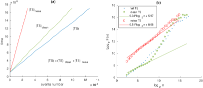
Figure 1: (a) clean $(TS)_{\text{clean}}$ and noise $(TS)_{\text{noise}}$ are produced by a BA filter (1) from an initial $(TS)_{\text{full}}$. (b) DFA results. Slope of the line is DFA scaling exponent $\alpha$ characterizing an impact of long term correlations.

Let $x$ be a random variable, and there is a finite series composed of $x$:

$$\{x_{1},x_{2},\dots,x_{N}\}.$$ (4)

In the case of DVS, there is a time series of events, and as a random variable $x$ stands a time interval $\delta t_{i}=t_{i}-t_{i-1}$ between adjacent events.

Let $X$ be a new random variable equal to a cumulative sum, $X_{1}=x_{1}$, $X_{2}=x_{1}+x_{2}$, $\dots$, $X_{N}=x_{1}+x_{2}+\dots+x_{N}$. Notice that for a DVS stream, the cumulative sums are exactly timestamps: $X_{i}=t_{i}$. Compose a cumulative series:

$$\{X_{1},X_{2},\dots,X_{N}\}.$$ (5)

Series (5) is partitioned in local segments of equal length $n$, and an independent least-square fit (local trend) is performed inside the $k$-th segment, $1\leq k\leq\lfloor N/n\rfloor$. Let $\hat{X}_{i}$ be the values predicted by a local trend, then, $(X_{i}-\hat{X}_{i})$ are detrended fluctuations. Mean local fluctuation of the $k$-th segment is:

$$F_{k}(n)=\left\{\frac{1}{n}\sum_{l=in+1}^{in+n}\left(X_{l}-\hat{X}_{l}\right)^{2}\right\}^{1/2},$$ (6)

and the mean total fluctuation depending on $n$ is averaged over all mean $k$ local fluctuations:

$$F(n)=\left\{\frac{1}{\lfloor N/n\rfloor}\sum_{k=1}^{\lfloor N/n\rfloor}F_{k}(n)^{2}\right\}^{1/2}.$$ (7)

The computation of eq. 6 and 7 run for segments of regularly increasing length $n\in\{m_{1},m_{2},\dots,m_{M}$}, where integers $m_{k}$ must obey the condition $m_{k}\simeq qm_{k-1}$, $q>1$ is a constant, i.e. $m_{k}$ must form a geometric progression, being $m_{1}=4$ and $m_{M}\simeq N$. As a result, a fluctuation function $F(n)$ is produced. If the series (4) is of long-range power-law correlations, $F(n)$ increases by a power-law:

$$F(n)\simeq Cn^{\alpha}.$$ (8)

The scaling exponent $\alpha$ gives a metric on self-correlations inside the initial series (4). To find $\alpha$, it is convenient to make double $\log n-\log F(n)$ plot as shown in Fig. 1b: $\alpha\simeq 0.5$ means uncorrelated data, $\alpha>0.5$ positive long-range correlations, $\alpha<0.5$ - anticorrelation, and $\alpha>1$ the data non-stationary [29], [30].

VI Results

To demonstrate how to assess objectively the quality of BA denoising without having a ground truth, we have used as noise input data a traditional dataset (slot-car dataset), and as filter we have adopted a commonly used basic filter in the field (Delbruck’s filter [7]). Even do our approach is not sensitive to hot pixels, to simplify the demonstration of our results without loosing in generality, hot pixels were removed form the input dataset.

Time bins from 4e6 till 16e6 with starting time 1e6 (all time units are in $\mu s$) are used. The time bin duration has no effect on the results, except for the longest (32e6) are better for the analysis (they provide more data for statistics), and short time bins are better for 3D $xyt$ visualisation (the long-time bins produce dirty 3D figures).

Fig.(2(a) - 2(h)) show BA denoising for different $\Delta T$ from 1000 till 16000. All the noise is removed well, but signal is removed too, as one can see easily in these 3D figures. It is easy to see signal traces in the filtered noise data because we are dealing with a simple dataset.

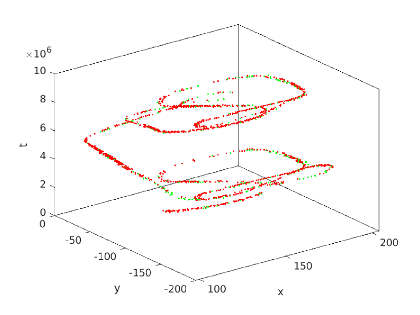
(a) $\Delta T=1000$ clean

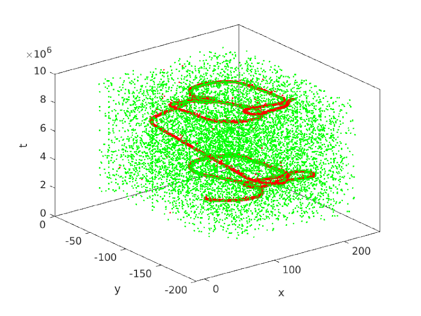
(b) $\Delta T=1000$ noise

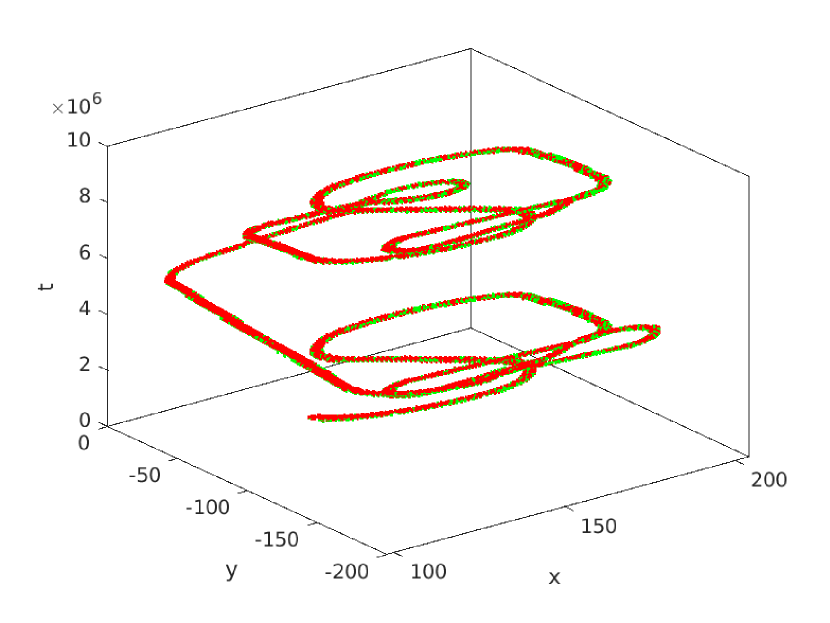
(c) $\Delta T=4000$ clean

(d) $\Delta T=4000$ noise

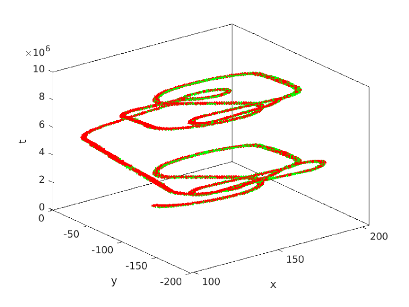
(e) $\Delta T=8000$ clean

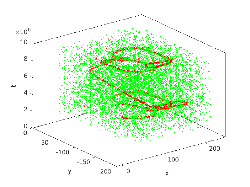
(f) $\Delta T=8000$ noise

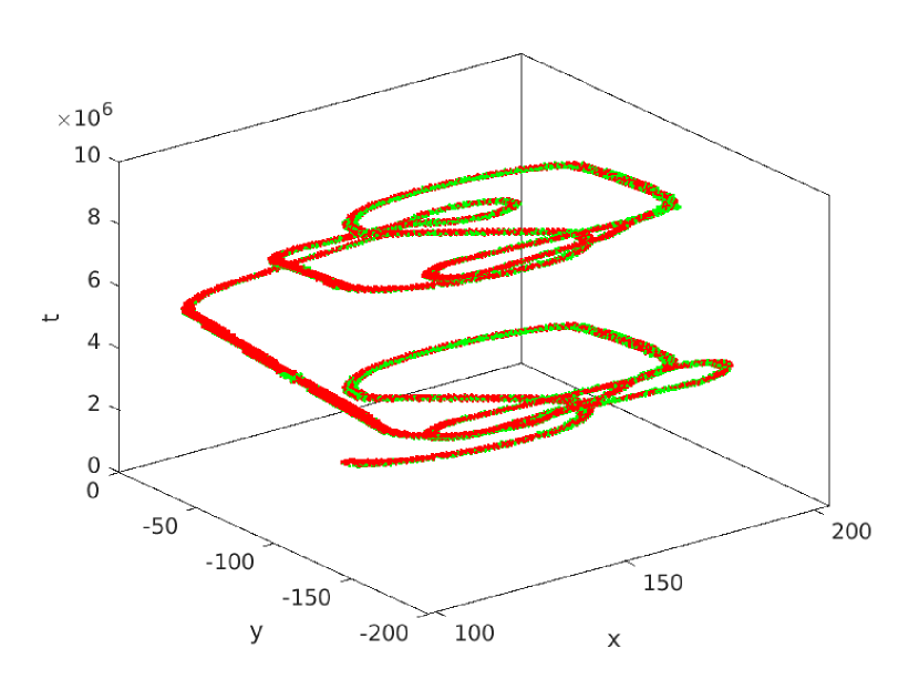
(g) $\Delta T=16000$ clean

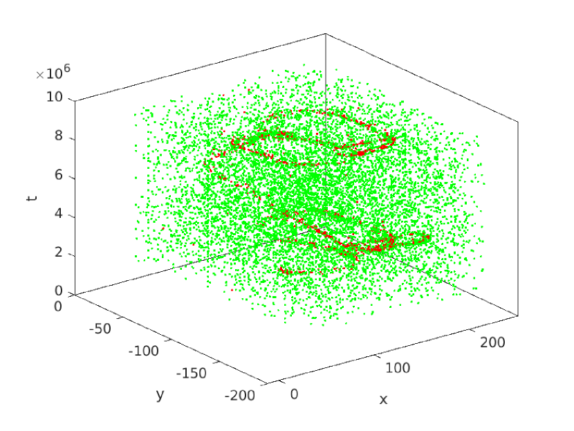
(h) $\Delta T=16000$ noise

Figure 2: BAF applied at various $\Delta T$.

Now we show how the signal captured by BA filter and manifested in the noise time series, disturbs noise statistical properties. Fig. 3 presents DFA results for the clean and noise time series at various $\Delta T$ shown in Fig.(2(a) - 2(h)). The DFA exponent $\alpha$ corresponds to the slope of crossover lines, see legend in Fig. 3b. At $\Delta T=1000$, $\alpha=0.74$ what is an evidence that noise is correlated, while $\alpha=0.50$ at $\Delta T=16000$ proves the filtered BA noise is random. Indeed, by comparing Fig. 2(b) with Fig. 2(h), one can see that in the first sample there are significant traces of spatially ordered signal in the noise time series, while in the second case, the signal traces are almost absent.

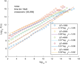
Figure 3: DFA applied to the noise time series.

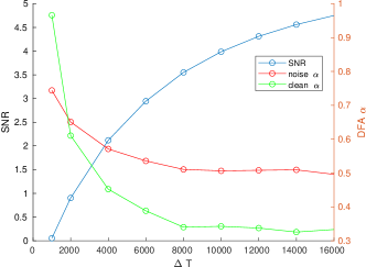
Figure 4: SNR and $\alpha$ as a function of $\Delta T$.

The Signal-Noise-Ratio (SNR) and DFA exponent $\alpha$ as a function of BA filter parameter $\Delta T$ are summarized in Fig. 4 to draw a conclusion that the BA filter $\Delta T$ for the slot-car data must be taken as large as possible since it provides the higher SNR with the $\alpha$ confirming random noise, and these both are asymptotically converging to their stationary values. This is trivial, since the highest SNR is of course better, however, such triviality is valid only for simple datasets, when BA noise is obviously random, i.e. we can easily distinguish in separate snapshots signal and noise as in the given example, and there is no doubt that suspected noise is random. Otherwise, noise long term correlations must be checked.

Now a question arise about how to select the optimal $\Delta T$. At larger $\Delta T$, BA filter works slower since the filter window captures more events. Each event in the window must be checked for correlations with the central event, i.e. a naive BA filter scales $O(N^{2})$ (there are technical implementations of BA filters free of this constrain, but then there appear other complexities). Then, we have two natural limits for BAF $\Delta T$: the lower $\Delta T$ is because of most events are treated as noisy but the filter is fast, and the higher limit is because of the finite computational resources. This is true already for simple scenes; for complex scenes one can not distinguish by eye all the details and separate suspected noise from the signal. Then, one can check statistical noise properties.

VII Conclusion

Detrended functional analysis (DFA) is presented to characterise quality of denoised DVS data without the availability of the ground truth. It is derived from statistical properties of filtered random noise extracted from a full DVS time series. The DFA is adapted to DVS data and tested with a popular slot-car dataset refined by a simple BA filter. It is demonstrated that DFA might be an useful tool since scaling exponents capture DVS signal in the filtered BA noise. As future works we would like to compare more complex BA filters, e.g., ynoise or knoise on complex datasets, such as data characterised by independently moving objects (IMO), where each object produces events with own statistical properties. Other possible future directions are for example, to explore how DFA exponents are linked with Poisson distribution of time intervals, investigate the possible outcome if instead of time intervals taken as random variable $x=t_{i}-t_{i-1}$, Eq.(4), one can consider the number of events $x=N$ coming inside some a priori fixed interval $\Delta t_{\text{ref}}$.

VIII Acknowledgment

This project has received funding from the European Union’s Horizon 2020 Research and Innovation Programme under Grant Agreement No 739578 and the Government of the Republic of Cyprus through the Deputy Ministry of Research, Innovation and Digital Policy.

References

- [1] G. Gallego, T. Delbrück, G. Orchard, C. Bartolozzi, B. Taba, A. Censi, S. Leutenegger, A. J. Davison, J. Conradt, K. Daniilidis, and D. Scaramuzza, “Event-based vision: A survey,” IEEE Transactions on Pattern Analysis and Machine Intelligence, vol. 44, no. 1, pp. 154–180, 2022.
- [2] G. Gallego, M. Gehrig, and D. Scaramuzza, “Focus is all you need: Loss functions for event-based vision,” 2019 IEEE/CVF Conference on Computer Vision and Pattern Recognition (CVPR), pp. 12 272–12 281, 2019.
- [3] M. Muglikar, M. Gehrig, D. Gehrig, and D. Scaramuzza, “How to calibrate your event camera,” 2021 IEEE/CVF Conference on Computer Vision and Pattern Recognition Workshops (CVPRW), pp. 1403–1409, 2021.
- [4] S. Shiba, Y. Aoki, and G. Gallego, “Secrets of event-based optical flow,” in European Conference on Computer Vision, 2022.
- [5] R. Graça, B. Mcreynolds, and T. Delbrück, “Optimal biasing and physical limits of dvs event noise,” ArXiv, vol. abs/2304.04019, 2023.
- [6] ——, “Shining light on the dvs pixel: A tutorial and discussion about biasing and optimization,” ArXiv, vol. abs/2304.04706, 2023.
- [7] T. Delbruck, “Frame-free dynamic digital vision,” in International Symposium on Secure-Life Electronics, vol. 1, no. 1. University of Tokyo, March 2008, pp. 21–26, in: Proceedings of International Symposium on Secure-Life Electronics, Advanced Electronics for Quality Life and Society, Univ. of Tokyo, Mar. 6-7, 2008. [Online]. Available: https://doi.org/10.5167/uzh-17620
- [8] H. Liu, C. Brandli, C. Li, S.-C. Liu, and T. Delbrück, “Design of a spatiotemporal correlation filter for event-based sensors,” 2015 IEEE International Symposium on Circuits and Systems (ISCAS), pp. 722–725, 2015.
- [9] S. J. Ding, J. Chen, Y. Wang, Y. Kang, W. Song, J. Cheng, and Y. Cao, “E-mlb: Multilevel benchmark for event-based camera denoising,” ArXiv, vol. abs/2303.11997, 2023. [Online]. Available: https://arxiv.org/abs/2303.11997
- [10] A. Khodamoradi and R. Kastner, “O(n)-space spatiotemporal filter for reducing noise in neuromorphic vision sensors,” IEEE Transactions on Emerging Topics in Computing, 2018.
- [11] S. Guo and T. Delbruck, “Low cost and latency event camera background activity denoising,” IEEE Transactions on Pattern Analysis and Machine Intelligence, 2022.
- [12] Y. Feng, H. Lv, H. Liu, Y. Zhang, Y. Xiao, and C. Han, “Event density based denoising method for dynamic vision sensor,” Applied Sciences, 2020.
- [13] X. Lagorce, G. Orchard, F. Galluppi, B. E. Shi, and R. B. Benosman, “Hots: a hierarchy of event-based time-surfaces for pattern recognition,” IEEE transactions on pattern analysis and machine intelligence, pp. 1346–1359, 2016.
- [14] R. W. Baldwin, M. Almatrafi, J. R. Kaufman, V. Asari, and K. Hirakawa, “Inceptive event time-surfaces for object classification using neuromorphic cameras,” in Image Analysis and Recognition, F. Karray, A. Campilho, and A. Yu, Eds. Cham: Springer International Publishing, 2019, pp. 395–403.
- [15] J. Wu, C. Ma, L. Li, W. Dong, and G. Shi, “Probabilistic undirected graph based denoising method for dynamic vision sensor,” IEEE Transactions on Multimedia, vol. 23, pp. 1148–1159, 2021.
- [16] R. W. Baldwin, M. Almatrafi, V. Asari, and K. Hirakawa, “Event probability mask (epm) and event denoising convolutional neural network (edncnn) for neuromorphic cameras,” 2020.
- [17] H. Fang, J. Wu, L. Li, J. Hou, W. Dong, and G. Shi, “Aednet: Asynchronous event denoising with spatial-temporal correlation among irregular data,” in Proceedings of the 30th ACM International Conference on Multimedia, ser. MM ’22. New York, NY, USA: Association for Computing Machinery, 2022, p. 1427–1435. [Online]. Available: https://doi.org/10.1145/3503161.3548048
- [18] G. Gallego, H. Rebecq, and D. Scaramuzza, “A unifying contrast maximization framework for event cameras, with applications to motion, depth, and optical flow estimation,” in 2018 IEEE/CVF Conference on Computer Vision and Pattern Recognition, 2018, pp. 3867–3876.
- [19] N. Xu, L. Wang, J. Zhao, and Z. Yao, “Denoising for dynamic vision sensor based on augmented spatiotemporal correlation,” IEEE Transactions on Circuits and Systems for Video Technology, vol. 33, no. 9, pp. 4812–4824, 2023.
- [20] C. Yang, H. Feng, Z. hai Xu, Q. Li, and Y. ting Chen, “The spatial correlation problem of noise in imaging deblurring and its solution,” J. Vis. Commun. Image Represent., vol. 56, pp. 167–176, 2018.
- [21] C.-K. Peng, S. V. Buldyrev, S. Havlin, M. Simons, H. E. Stanley, and A. L. Goldberger, “Mosaic organization of dna nucleotides,” Phys. Rev. E, vol. 49, pp. 1685–1689, Feb 1994. [Online]. Available: https://link.aps.org/doi/10.1103/PhysRevE.49.1685
- [22] B. Rogers, D. Giles, N. Draper, O. Hoos, and T. Gronwald, “A new detection method defining the aerobic threshold for endurance exercise and training prescription based on fractal correlation properties of heart rate variability,” Front. Physiol., vol. 11, p. 596567, 2020.
- [23] T. Kataoka, T. Miyaguchi, and T. Akimoto, “Detrended fluctuation analysis of earthquake data,” Phys. Rev. Res., vol. 3, p. 033081, Jul 2021. [Online]. Available: https://link.aps.org/doi/10.1103/PhysRevResearch.3.033081
- [24] X. Gou, M. Chen, and G. Zhang, “Time correlations of lightning flash sequences in thunderstorms revealed by fractal analysis,” Journal of Geophysical Research: Atmospheres, vol. 123, no. 2, pp. 1351–1362, 2018. [Online]. Available: https://agupubs.onlinelibrary.wiley.com/doi/abs/10.1002/2017JD027206
- [25] K. Shrestha, “Multifractal detrended fluctuation analysis of return on bitcoin*,” International Review of Finance, vol. 21, no. 1, pp. 312–323, 2021. [Online]. Available: https://onlinelibrary.wiley.com/doi/abs/10.1111/irfi.12256
- [26] J. Alvarez-Ramirez, E. Rodriguez, I. Cervantes, and J. Carlos Echeverria, “Scaling properties of image textures: A detrending fluctuation analysis approach,” Physica A: Statistical Mechanics and its Applications, vol. 361, no. 2, pp. 677–698, 2006. [Online]. Available: https://www.sciencedirect.com/science/article/pii/S0378437105007193
- [27] K. Hu, P. C. Ivanov, Z. Chen, P. Carpena, and H. Eugene Stanley, “Effect of trends on detrended fluctuation analysis,” Physical Review E, vol. 64, no. 1, Jun. 2001. [Online]. Available: http://dx.doi.org/10.1103/PhysRevE.64.011114
- [28] J. W. Kantelhardt, E. Koscielny-Bunde, H. H. Rego, S. Havlin, and A. Bunde, “Detecting long-range correlations with detrended fluctuation analysis,” Physica A: Statistical Mechanics and its Applications, vol. 295, no. 3, pp. 441–454, 2001. [Online]. Available: https://www.sciencedirect.com/science/article/pii/S0378437101001443
- [29] M. S. Taqqu, V. Teverovsky, and W. Willinger, “Estimators for long-range dependence: An empirical study,” Fractals, vol. 03, no. 04, pp. 785–798, 1995. [Online]. Available: https://doi.org/10.1142/S0218348X95000692
- [30] M. Höll, K. Kiyono, and H. Kantz, “Theoretical foundation of detrending methods for fluctuation analysis such as detrended fluctuation analysis and detrending moving average,” Phys. Rev. E, vol. 99, p. 033305, Mar 2019. [Online]. Available: https://link.aps.org/doi/10.1103/PhysRevE.99.033305
- [31] L. Kristoufek, “Detrending moving-average cross-correlation coefficient: Measuring cross-correlations between non-stationary series,” Physica A: Statistical Mechanics and its Applications, vol. 406, pp. 169–175, 2014. [Online]. Available: https://www.sciencedirect.com/science/article/pii/S037843711400209X