Toward Efficient Visual Gyroscopes: Spherical Moments, Harmonics Filtering, and Masking Techniques for Spherical Camera Applications

Abstract

Unlike a traditional gyroscope, a visual gyroscope estimates camera rotation through images. The integration of omnidirectional cameras, offering a larger field of view compared to traditional RGB cameras, has proven to yield more accurate and robust results. However, challenges arise in situations that lack features, have substantial noise causing significant errors, and where certain features in the images lack sufficient strength, leading to less precise prediction results.

Here, we address these challenges by introducing a novel visual gyroscope, which combines an analytical method with a neural network approach to provide a more efficient and accurate rotation estimation from spherical images. The presented method relies on three key contributions: an adapted analytical approach to compute the spherical moments coefficients, introduction of masks for better global feature representation, and the use of a multilayer perceptron to adaptively choose the best combination of masks and filters. Experimental results demonstrate superior performance of the proposed approach in terms of accuracy. The paper emphasizes the advantages of integrating machine learning to optimize analytical solutions, discusses limitations, and suggests directions for future research.

I INTRODUCTION

A classical problem in robotics is the estimation of the orientation of a camera. By analyzing the features of two or more consecutive images, a Visual Gyroscope (VG) can determine the orientation and angles of the camera, instead of relying on mechanical structures like traditional gyroscopes. With its ability to provide precise measurements and real-time tracking  [1, 2], the visual gyroscope is a powerful tool for a wide range of industries and fields, from stabilizing cameras and drones to navigating autonomous vehicles and spacecraft.

Traditionally, visual gyroscopes have utilized various types of sensors, estimation methods, and feature extraction techniques. Employed sensors include monocular cameras [3], stereo cameras [4], panoramic cameras [5], RGB-D cameras [6], or combinations thereof [7].

The utilization of omnidirectional cameras has emerged, as a recent area of investigation within the realm of visual navigation for mobile robotics and autonomous systems. With the advent of omnidirectional cameras, a VG is capable of capturing a full 360-degree view of the surroundings, and researchers are starting to develop accurate and real-time spherical visual gyroscopes.

Conventionally, most existing visual gyroscope methods have been based on extended Kalman filters (EKF) [8, 9], sequential Monte Carlo methods, particle filters (PF) [10, 11, 12], optical flow [13, 14, 15], feature-based [16, 17], or even Fourier transform based methods [18, 19].

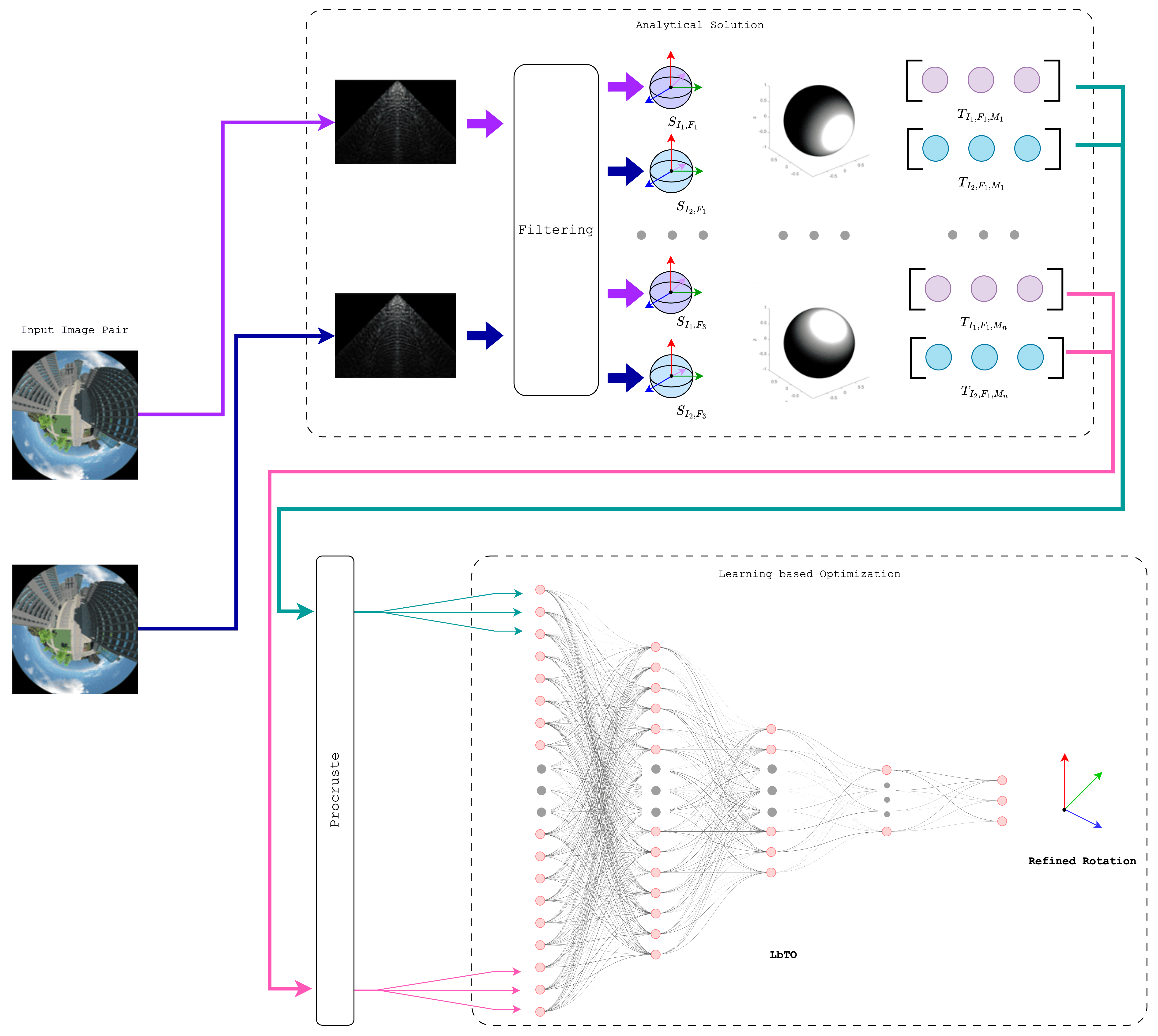
Figure 1: Overview of the novel efficient visual gyroscope. The proposed visual gyroscope method consists of two key computation blocks: the analytical computation of the spherical moment triplets and the learning-based triplet optimization, which conjunctively lead to a more accurate and efficient final image rotation estimation.

Most of the methods above encompass non-linear state equations and non-Gaussian noise assumptions, which impact the resulting accuracy and efficiency. In addition, these approaches demand greater computational and memory resources, while also being sensitive to minor changes in dynamic environments.

To address these challenges, this paper proposes a novel method, the Fast Visual Gyroscope (FVG), which computes more accurate and efficient 3D orientations of the camera for a given image with respect to a reference. As illustrated in Fig. 1, the FVG approach consists of two parts: an analytical solution from the Procrustes analysis of two sets of triplets from different images, and an additional optimization method that uses machine learning to optimize the final rotation estimations. Our approach offers a faster and more accurate computation of rotation estimates thanks to the efficiency gain from the new analytical step and the accuracy gain from the learning-based optimization of rotation estimates. The efficacy of our method was demonstrated against a baseline visual gyroscope method [10], highlighting the advantages of the fast visual gyroscope.

II Related Works

According to different operating principles, visual gyroscopes can be divided into different categories, including but not limited to the ones based on optical flow [13, 15], using image features [16, 17], Fourier transform [18, 19], particle filtering [10, 20] and hybrid solutions [21, 22].

The extended Kalman filter [23] is a tracking framework that linearizes measurements and evolution models through Taylor series expansions [18, 19]. Jiang et al. [24] introduced an EKF tracking approach utilizing pre-calibrated fiducials for initiation and achieving extendable tracking through dynamic calibration of line features. Kyrki et al. [8] integrated model-based and model-free cues using EKF but faced robustness issues with outliers, while Kragic et al. [9] extended their work by developing a method for automatic initialization of pose tracking based on robust feature matching.

The approximation in EKF can lead to poor representations of the nonlinear functions and probability distributions of interest. The sequential Monte Carlo method, or particle filters [10] could provide improved robustness over the Kalman filters. Qian et al. [25] describe an ad-hoc method for incorporating gyroscope measurements by sampling the rotation angles according to the measured angular velocities while applying a random walk to the position. Schon et al. [11] presented the marginalised particle filter (MPF) with concepts like automatic model-switching, improved orientation proposals, adaptive process noise and mixture proposals. Sadghzadeh et al. [12] employ the Bayesian based PF approach to estimate inertia tensor due to nonlinear and non-Gaussian models.

Optical flow represents the distribution of apparent velocities of brightness patterns in an image [13, 15, 26], and is used to estimate the projected motion of the relative displacement between the camera and the objects.

Feature-based gyroscopes [27, 16, 28, 17] use the detection and tracking of distinctive image features, such as corners, edges, or blobs, to estimate rotation. They can achieve higher accuracy and robustness than optical flow gyroscopes, but require more computation and memory resources. Feature-based gyroscopes are commonly used in robotics, augmented reality, or autonomous vehicles.

However, optical flow or feature-based methods are easily affected by small changes in the dynamic environment, as well as when the images change significantly (such as in the case of large movements) [19]. Based on harmonic analysis [29, 30], Makadia et al. [31] proposes a framework for studying image deformation applicable in the plane and on the sphere. These deformations have also been explored in learning-based methods [32, 33, 34] and have achieved great results. Similarly, Burel et al. [35] determine the 3D orientation from normalizing tensors which are obtained from spherical harmonics coefficients. Chirikjian et al. [29] shows good applications using this method.

Visual gyroscope technology using cameras has found wide applications in navigation, robotics, and augmented reality. The use of this technology is important as it enables accurate and responsive navigation thanks to the real-time tracking of changes in orientation.

Despite its benefits, there are also some challenges. These include reliance on visual features, which can be a challenge in low-light or featureless environments. The accuracy of visual gyroscope technology can also be affected by the position and orientation of the camera, as well as the distance and angle between the camera and the visual features in the environment.

Additionally, visual gyroscope technology requires significant processing power to analyze camera images and track visual features, which can be a challenge for low-power devices. Furthermore, accurate calibration of camera and computer vision algorithms is essential for precise orientation determination, and this process can be complex and time-consuming.

III Contribution

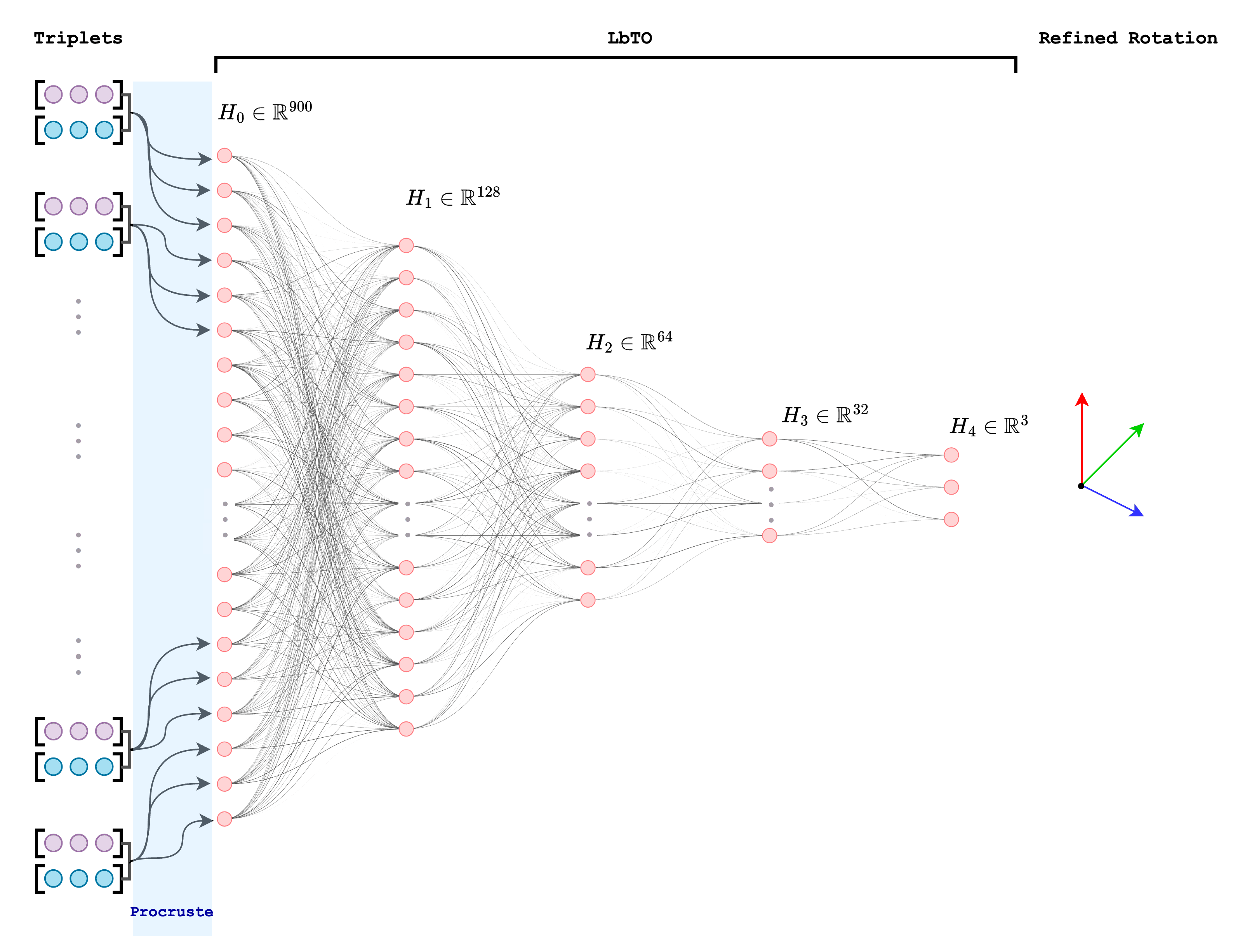
Figure 5: Input and structure of the proposed learning-based triplet optimizer. Given the input spherical moment triplets, rotations are obtained from triplets using procrustes analysis, and are then fed into an MLP to get refined rotation estimations. The supervised training of the MLP results in the number and type of filters and masks being optimized to get optimal rotation predictions.

In this paper, we designed a visual gyroscope to estimate 3D rotation using as input only spherical images. The overview of this algorithm is shown in Fig. 2 and Fig. 5.

The proposed fast visual gyroscope consists of an analytical step and a multi-layer perceptron (MLP) model, which is particularly noteworthy as it utilizes raw rotation estimates from analytical solutions as input. These unique features are extracted from spherical harmonics coefficients of spherical images, which are transformed into the frequency domain and filtered to enhance the number of features.

To ensure the equivariance property of the used feature, a multi-mask strategy is employed to reduce the influence of non-overlapping parts in different images, which is directly applied through the combination of different orders of spherical harmonics. Additionally, spherical moments are calculated from both filtered and original spherical harmonics coefficients.

The network is trained using a simulated scenario proposed in [36], with data augmentation implemented through a folder-sliding window structure algorithm to increase motion sampling.

Finally, the proposed pipeline is tested on experiments, providing a comprehensive evaluation of its efficacy. The innovative use of raw rotation input and spherical harmonics coefficients make the proposed fast visual gyroscope model a significant advancement in the field. The multi-mask strategy ensures the preservation of equivariance property, while data augmentation and filtering techniques enhance the features. This work provides a valuable contribution to the development of effective models for analyzing robotic movements.

IV Methods

According to the pipeline (Fig. 1) proposed in this paper, the initial step involves transforming the spherical image into the spherical harmonics domain, followed by filtering operations within this domain. Subsequently, spherical moments are directly computed in the spherical harmonics domain. The calculated spherical moments are then combined linearly to obtain masked spherical moments. Next, a rotation estimate is derived from the masked spherical moments, and this estimation is utilized as input for optimizing a multilayer perceptron.

Here we describe in more detail the three crucial steps of our algorithm. The first part introduces a rapid method for directly computing spherical moments in the spherical harmonics domain. The second part outlines the approach of obtaining masked spherical moments through linear combinations. The third part explores the structure of the MLP, loss functions, and training strategies.

IV-A From Spherical Harmonics to Spherical Moments

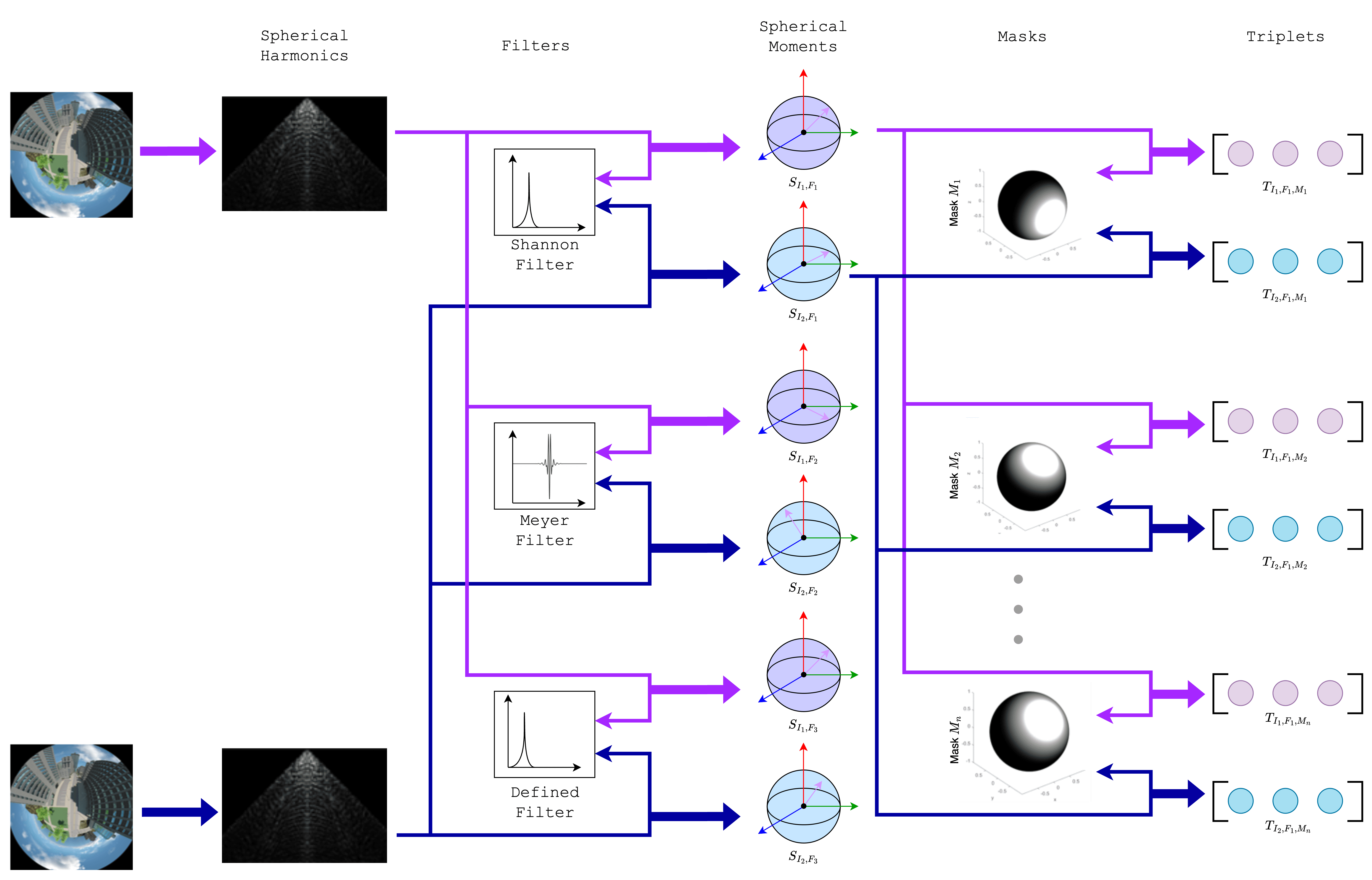
Figure 2: Image pre-processing for the analytical computation of triplets derived from spherical moments. First filtering and masking (total of 100 masks) are applied to the images, and then the spherical moments are computed before the feature triplets.

Generally, the method to compute spherical moments is composed of two steps: firstly, the image in the frequency domain is transformed to the spatial domain, via the inverse Fourier transform. Secondly, the image is projected onto a sphere, and then the spherical moments of the image are calculated.

Originally, spherical moments in image domain is defined as follows:

$$m_{ijk}=\iint_{s}x_{s}^{i}y_{s}^{j}z_{s}^{k}I(s)ds.$$ (1)

Thus, moments are computed as the integral of the image over the surface of an unitary sphere. But if the spherical moment could be directly calculated from the spherical harmonic coefficients, the calculation speed would be accelerated. The definition of spherical harmonics coefficients $\hat{I}_{lm}$:

$$\hat{I}_{lm}=\iint_{s}I(s)Y_{lm}^{*}(s)ds,$$ (2)

where $Y_{lm}^{*}$ is the conjugate of spherical harmonics of degree $l$ and order $m$ (integer between $-l$ and $l$), $I$ is original image over the unity sphere surface $s=(\theta,\varphi)$.

The calculation of $Y_{lm}$ is given by the following formula:

$$Y_{lm}(\theta,\phi)=(-1)^{m}\sqrt{\frac{2l+1}{4\pi}\frac{(l-m)!}{(l+m)!}}P_{l}^{m}(\cos\theta)e^{im\phi}=\Psi,$$ (3)

where $\theta$ is the elevation angle, $\phi$ is the azimuthal angle, $P_{l}^{m}(\cos\theta)$ is the associated Legendre polynomial, and $i$ is the imaginary unit.

The associated Legendre polynomial $P_{l}^{m}(\cos\theta)$ can be calculated using the recursion formula:

$$\begin{split}&(l-m+1)P_{l+1}^{m}(\cos\theta)-(l+m)P_{l}^{m}(\cos\theta)+\\ &(l+m)\frac{(l-m+1)}{\sin\theta}P_{l}^{m-1}(\cos\theta)=0,\end{split}$$ (4)

with the following initial conditions,

$$\begin{cases}P_{l}^{l}(\cos\theta)=(-1)^{l}(2l-1)!!\gamma\\ P_{l}^{-l}(\cos\theta)=(-1)^{l}\frac{(2l-1)!!}{(2l)!!}\gamma^{m/2}\frac{d^{|m|}}{d(\cos\theta)^{|m|}}(-\gamma)^{l}\end{cases},$$ (5)

where $\gamma=(1-\cos^{2}\theta)$. The normalization factor $\sqrt{\frac{2l+1}{4\pi}\frac{(l-m)!}{(l+m)!}}$ in equation (3) ensures that the spherical harmonics are orthonormal.

Substituting the solution for $I(s)$ from equation (2) into equation (1), the spherical moments can be computed from spherical harmonics coefficients as:

$$m_{ijk} =\sum_{l}\sum_{m}\iint_{s}x^{i}y^{j}z^{k}\hat{I}_{lm}\Psi ds,$$ (6)

$$=\sum_{l}\sum_{m}\hat{I}_{lm}\iint_{s}x^{i}y^{j}z^{k}\Psi ds,$$

$$=\sum_{l}\sum_{m}\hat{I}_{lm}C^{ijk}_{lm},$$

where we derive the moments coefficient equation in frequency domain as:

$$\small{\begin{array}[]{ll}\begin{aligned} C_{lm}^{ijk}&=\iint_{s}x^{i}y^{j}z^{k}\Psi ds,\\ &=\iint_{s}(r\sin\theta\cos\varphi)^{i}(r\sin\theta\sin\varphi)^{j}(r\cos\theta)^{k}\Psi ds,\\ &=\iint_{s}(\sin\theta)^{i+j}\cos\varphi^{i}\sin\varphi^{j}\cos\theta^{k}\Psi\sin\theta d\theta d\varphi,\\ &=\iint_{s}(\sin\theta)^{i+j+1}\cos\varphi^{i}\sin\varphi^{j}\cos\theta^{k}\Psi d\theta d\varphi.\end{aligned}\end{array}}$$ (7)

where, as a recall, $\Psi=Y_{lm}(\theta,\varphi)$.

Equation (6) provides our analytical closed-form expression for the set of spherical moment coefficients of different orders. This new analytical expression transforms convolution and integration operations into a multiplication operation, thus greatly reducing the computational complexity of the final expression. Furthermore, since the function $C_{lm}^{ijk}$ that we introduce is a basis function, we can reduce computational complexity by storing the values for each needed $(l,m,i,j,k)$ tuple.

IV-B Fast Implementation of Mask on Spherical Moments

A known common issue when using visual gyroscopes for the estimation of rotation on global features is that the presence of non-overlapping regions in two images could reduce the accuracy in ego-motion visual estimation. Since our analytical expression (6) would suffer from this problem as well, we propose the use of different masks to reduce the influence of non-overlapping regions before calculating the triplets.

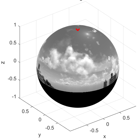
(a)

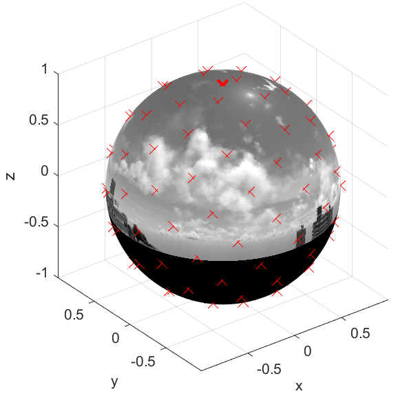
(b)

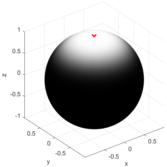
(c)

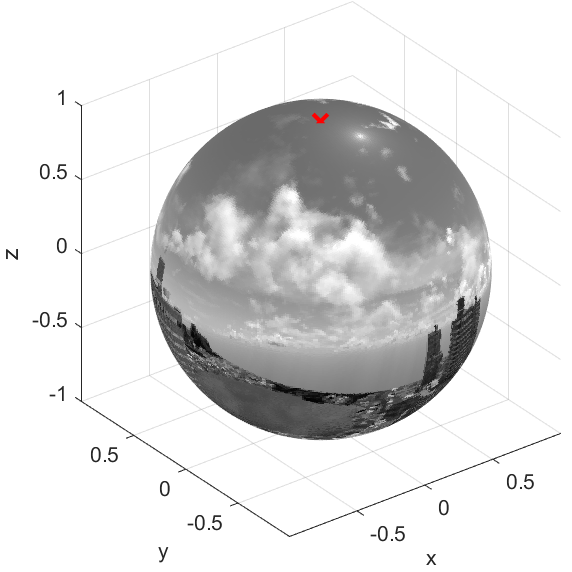
(d)

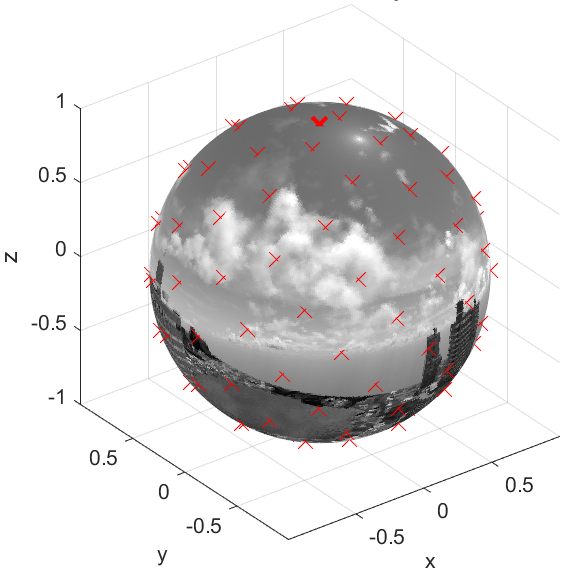
(e)

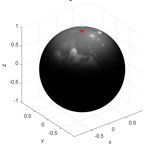
(f)

Figure 3: Masking method explained. (a) and (d) show the images on a half sphere and around the complete spherical surface. (b) presents an icosahedral sample delicately positioned on a half sphere. The figure (e) extends its scope to showcase the icosahedral sample enveloping the entire surface of a sphere. (c) and (f) introduce a mask on a sphere and an image overlaid with a mask.

A sampling method uniformly distributed according to azimuth and elevation will result in too many sampling points close to the poles and too few sampling points near the equator. Therefore, we used the sampling method of icosahedral distribution to avoid this problem as shown in Fig. 3.

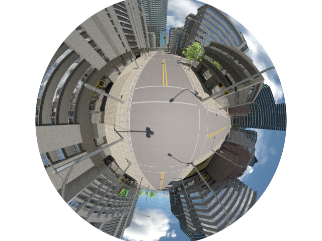
(a)

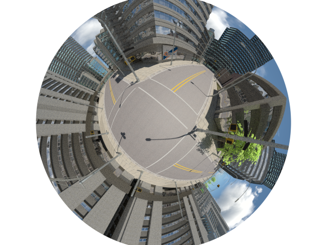
(b)

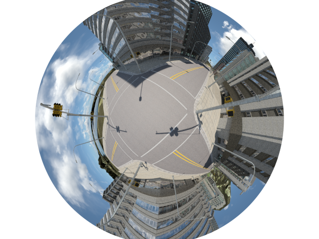
(c)

Figure 4: Images generated from the Blender simulation environment. We generate 500 images for the training and 150 for the testing of the MLP, by randomly sampling the rotation metrics. (a)-(c) show three examples of the generated images.

Taking into account the targeted application, a well adapted mask is the one of a round shape, with the weight 1 around the region center, and decreasing softly around the region border. Inspired by [37], a good candidate that holds these conditions is defined as:

$$\begin{cases}W(z_{s})=0&\left(-1<z_{s}<z_{0}-r\right)\\ W(z_{s})=e^{-\frac{\left(z-\left(z_{0}+r\right)\right)^{2}}{\sigma^{2}}}&\left(z_{0}-r\leq z_{s}\leq z_{0}+r\right)\\ W(z_{s})=1&\left(z_{0}+r<z_{s}<1\right)\\ \end{cases}.$$ (8)

The mask’s shape is determined by parameters $\sigma$ and range $r$, while $z_{0}$ represents the center of the mask. Such a shape is well adapted to recover the rotation around the z-axis. However, its formulation is quite complex for computing moments corresponding to the selected region. Instead of using equation (8), masks under polynomial form on the variate $z_{s}$ can be used:

$$W(x,y,z)=\sum_{l=0}^{n}\sum_{m=0}^{n}\sum_{p=0}^{n}a_{lmp}\cdot x^{l}\cdot y^{m}\cdot z^{p},$$ (9)

where $a_{lmp}$ are the coefficient of the polynomial. They are defined such that the equation (9) approximates the shape of the mask defined by the equation (8). According to the equation (1) and the equation (2):

$$m_{ijk}^{mask} =\sum_{l}\sum_{m}\iint_{s}x^{i}y^{j}z^{k}\hat{I}_{lm}e^{-\left(\frac{z-z_{0}}{\sigma}\right)^{g}}\Psi ds,$$ (10)

$$=\sum_{l}\sum_{m}\hat{I}_{lm}\iint_{s}x^{i}y^{j}z^{k}\sum_{h=0}^{\infty}\frac{\left(\frac{z-z_{0}}{\sigma}\right)^{gh}}{h!}\Psi ds,$$

$$=\sum_{l}\sum_{m}\hat{I}_{lm}\Upsilon_{mask}^{ijk},$$

where the coefficient can be replaced as:

$$\Upsilon_{mask}^{ijk} =\tiny{\iint_{s}x^{i}y^{j}z^{k}\Psi ds},$$ (11)

$$=\tiny{\iint_{s}(r\sin\theta\cos\varphi)^{i}(r\sin\theta\sin\varphi)^{j}(r\cos\theta)^{k}\Psi ds},$$

$$=\tiny{\iint_{s}x^{i}y^{j}z^{k}\Psi\sum_{h=0}^{\infty}\frac{\left(\frac{z-z_{0}}{\sigma}\right)^{gh}}{h!}ds}.$$

For the last sum part and the item with $z^{k}$:

$$z^{k}\sum_{h=0}^{\infty}\frac{\left(\frac{z-z_{0}}{\sigma}\right)^{gh}}{h!},$$ (12)

can be written as a linear combination of $z^{p}$, namely:

$$z^{k}\sum_{h=0}^{\infty}\frac{\left(\frac{z-z_{0}}{\sigma}\right)^{gh}}{h!}=\sum_{p=k}^{k+q}a_{p}z^{p}.$$ (13)

Therefore, we can get the coefficient with a mask from a linear combination of the higher order coefficients without the mask:

$$\Upsilon_{mask}^{ijk} =\iint_{s}x^{i}y^{j}\Psi\sum_{p=k}^{k+q}a_{i}z^{p}ds,$$ (14)

$$=\sum_{p=k}^{k+q}a_{i}\iint_{s}x^{i}y^{j}z^{p}\Psi ds,$$

$$=\sum_{p=k}^{k+q}C^{ijk}_{lm}.$$

Using the coefficient $\Upsilon_{mask}^{ijk}$ of spherical moments, it is possible to directly obtain masked spherical moments and subsequently calculate a set of triplet features. These triplet features provide valuable information about the relative positions and orientations of objects, which can aid in rotation estimation. With the set of triplet features, it is possible to obtain an analytical solution for rotation estimation. This solution can be further enhanced using various techniques, such as regularization or noise modeling, to improve its accuracy and robustness.

Overall, by leveraging the coefficient $\Upsilon_{mask}^{ijk}$ of spherical moments, one can obtain both spherical moments and triplet features, which can be used to obtain a reliable and accurate analytical solution for rotation estimation.

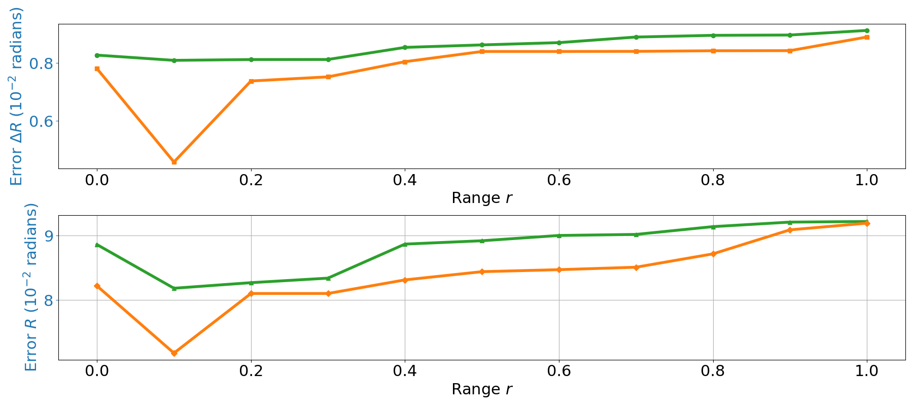
(a)

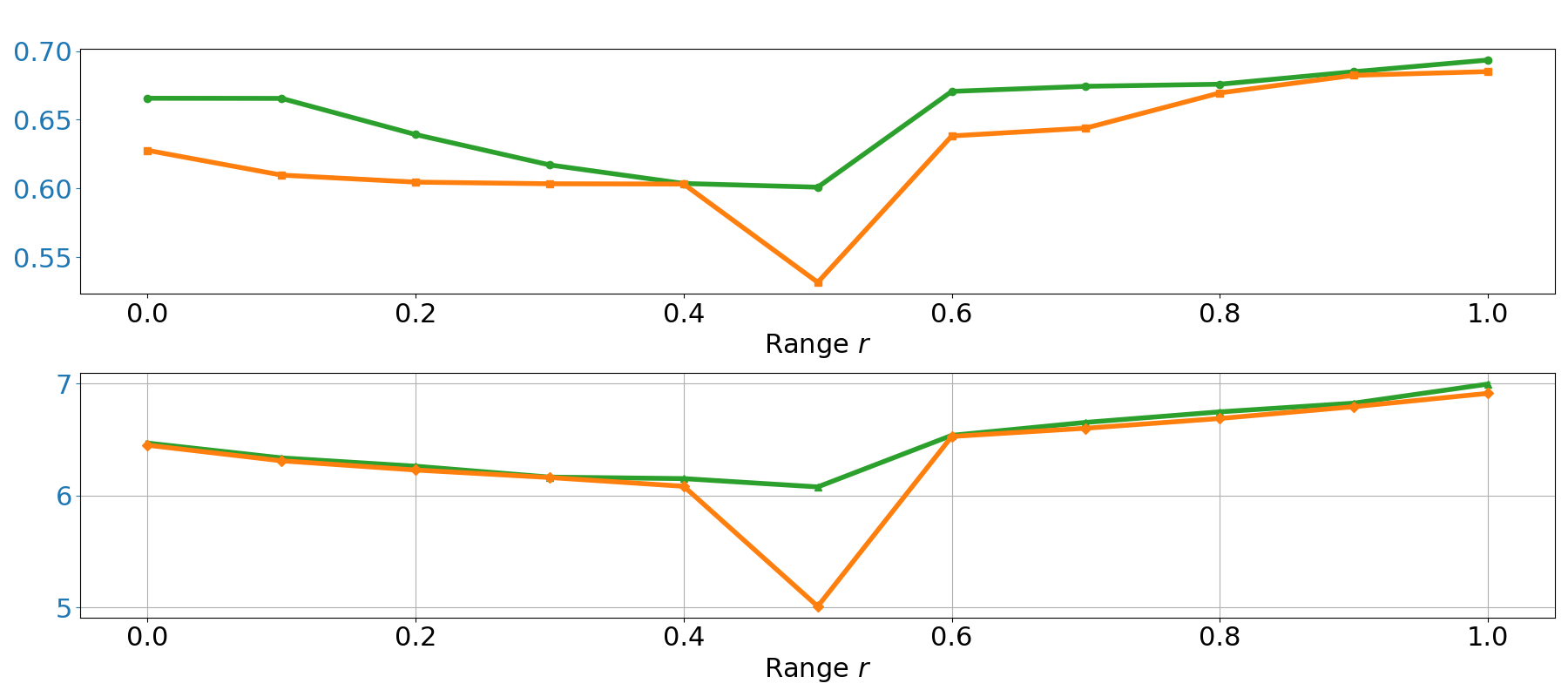
(b)

Figure 6: Analysis of the impact of mask range on the accuracy of rotation estimations. The full analytical-LbTO method (fast visual gyroscope) is compared to the analytical method alone, to reveal optimal range value and significantly higher accuracy of our proposed analytical-LbTO method. (a) displays the comparison of error for various values of the range $r$ in a pure rotation sequence with half sphere images, (b) shows comparison of error for various values of the range $r$ in pure rotation sequence with whole sphere image.

IV-C LbTO: Learning-based Triplet Optimizer

To further increase the accuracy of the predicted rotation estimation on spherical images, we introduce the third and last step in our method: a neural network based optimization of the type and number of masks and filters. Specifically, we train an MLP to choose the masks and filters that minimize the error between the predicted and ground truth rotation vectors. The MLP is trained and tested with synthesized fisheye camera data from Blender as shown in Fig. 4.

In terms of the neural network architecture, we use a three-layer 128x64x32 MLP (excluding input and output layers). During the training process, we combine a decaying learning rate, SWA learning rate schedules, and the Adam optimizer in order to accelerate the MLP learning convergence, prevent overfitting, and enhance the generalization performance. And for the loss function we use Mean Squared Error (MSE).

Addressing the challenge of discontinuity in MSE loss functions requires careful consideration of degrees of freedom (DoF). While augmenting DoF presents a potential solution, it necessitates careful balance due to its impact on training time and real-time performance. For instance, Zhou et al. [38] proposed 5D and 6D continuous representations to mitigate discontinuity issues in computer vision deep learning approaches, focusing exclusively on rotational aspects. However, considering our emphasis on estimating rotations between adjacent images, where estimates typically hover near zero, we opt for the axis-angle representation. This choice ensures practicality without compromising accuracy, aligning seamlessly with the objectives of our study.

V Experiments

Due to the potential for errors in the ground truth caused by temperature drift and zero drift in the inertial measurement unit in real-world environments, all experiments are conducted in the Blender simulation environment.

The experiment involves pure 3D rotation motion, which tests the algorithm’s ability to estimate rotation accurately without the influence of other factors.

We perform the experiment with a dataset generated in the Blender simulation environment, which consisted of 500 images, 30% of which are used for testing and 70% for training. The rapidity of our proposed fast visual gyroscope method is demonstrated by its implementation with 100 masks, taking only 20 milliseconds to apply all masks.

To study the impact of the learning based optimization step in our three-step visual gyroscope approach, we conduct an experiment in which we evaluate the impact of the range on the accuracy of predicted rotation estimates. Our experiment demonstrates the criticality of the learning based optimization, which leads to a much more accurate rotation estimation than had we used the analytical steps alone. Fig. 6(a) shows that when only half of the spherical image is available, we can determine that $r=0.1$ is the optimal choice for minimizing errors through empirical experimentation with different range values. In this case, selecting a mask with a smaller radius is beneficial to prevent interference from the edges of the spherical image, which can lead to errors. This approach is effective for estimating both the rotation difference, $\Delta R$, and the overall rotation, $R$, between two images.

The rationale behind this finding is that when considering only half of the sphere, the value $r=0.1$ ensures that the mask does not extend to the boundaries of the spherical image. If we were to increase the value of $r$ further, the impact of the spherical image boundaries on error would become more significant relative to the reduction in error achieved by expanding the field of view. Therefore, the choice of $r=0.1$ strikes a balance between these two effects, ultimately minimizing the error.

Similarly, the data in Fig. 6(b) clearly indicates that when considering the entire spherical surface, through experimentation with different range values, we can ascertain that $r=0.5$ emerges as the most effective choice for minimizing errors. This conclusion holds true not only for the estimation of rotation $\Delta R$ but also for the cumulative rotation estimation $R$ between two images.

The rationale behind this outcome remains consistent with the prior scenario. When dealing with the entire spherical surface, the value $r=0.5$ notably amplifies the reduction in error achieved through the expansion of the field of view. This reaffirms the earlier theory that $r=0.1$ minimizes the error on the half spherical surface. It is worth noting that the analytical solution method can suffer from inaccuracies due to its dependence on the used masks. However, the results obtained using the LbTO are closer to the ground truth, indicating the effectiveness of the proposed approach in estimating the rotation angles. This conclusion is crucial for our problem, as it helps determine the optimal parameter configuration to achieve as accurate a rotation estimation as possible. Such analysis contributes to improving the performance and accuracy of image processing algorithms.

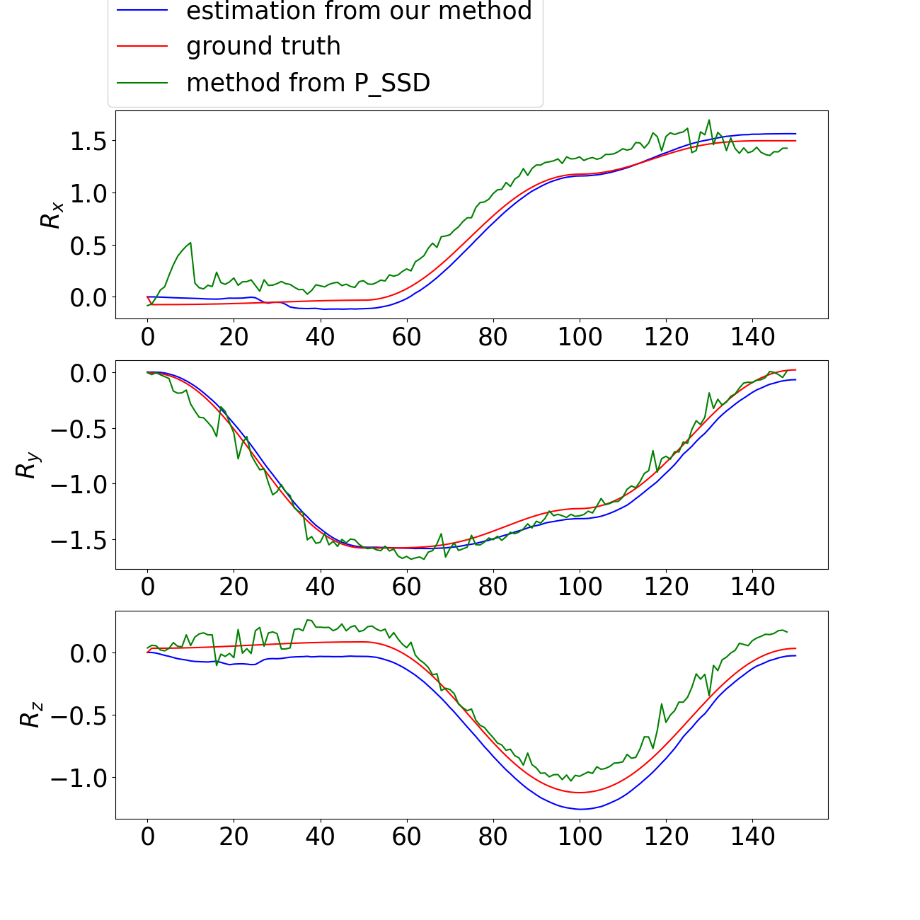
(a)

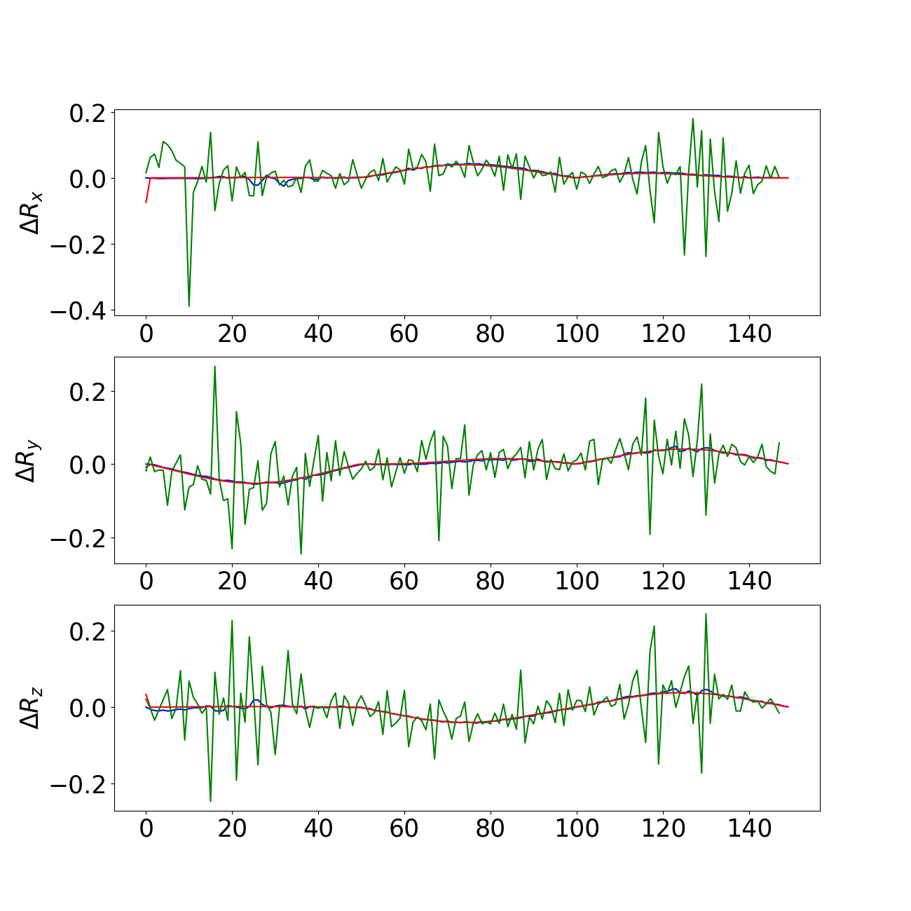
(b)

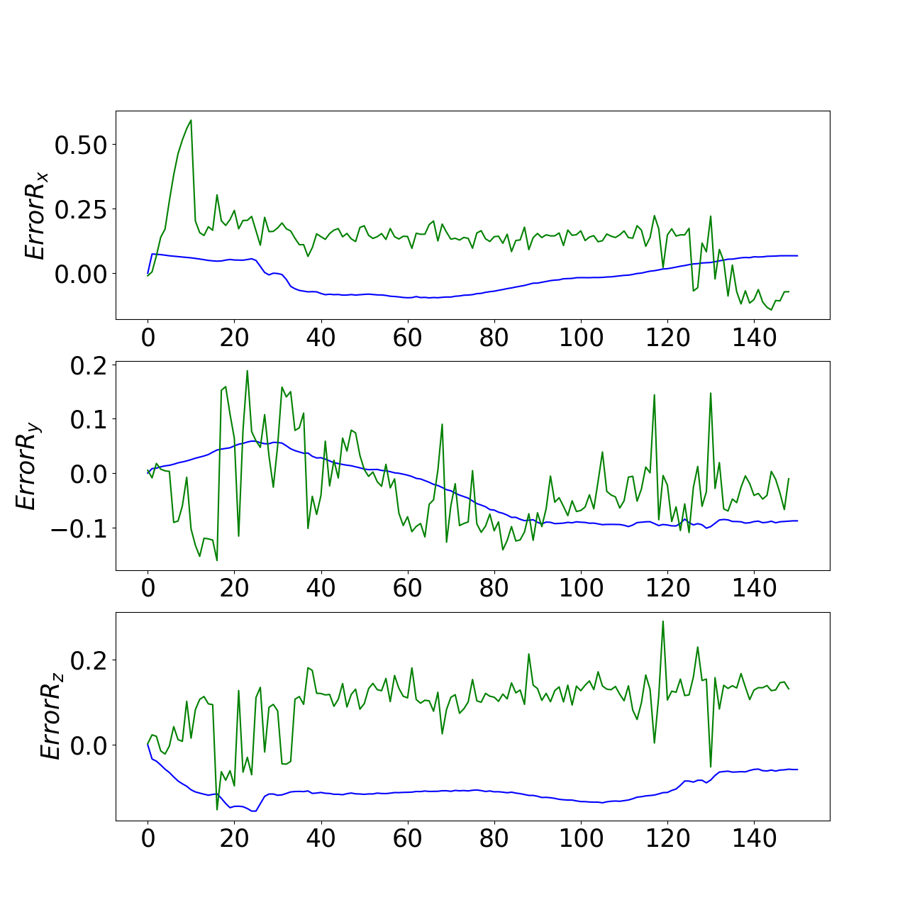
(c)

Figure 7: Performance benchmark against ground-truth data and baseline VG approach in a simulated environment. Our proposed analytical-LbTO VG method is evaluated against a baseline VG approach [7] to reveal higher accuracy and less noisy predictions. (a) Comparison of different approaches to estimate $\theta$, (b): Comparison of different approaches to estimate $\Delta\theta$, (c): The error of estimating the rotation angle. All comparisons are done along the three spatial axes for our method and the baseline VG method with ground-truth data shown for reference. The $x$, $y$, and $z$ rotations are expressed in terms of axis angles and plotted against the image number on the $x$-axis and the angle of rotation in radians on the $y$-axis.

Fig. 7 displays the results of comparison with the method from [5], which introduces a new visual gyroscope named P_SDD using dual-fisheye cameras to accurately estimate orientation by projecting images onto a sphere.

The same conclusion can be drawn in Fig. 7(b), which shows the rotations between 2 images. Fig. 7(c) depicts the errors in estimation, which further confirm the effectiveness of the neural network model in accurately estimating the rotation.

Our method proves to be more reliable compared to P_SDD, which exhibits much higher error varability when estimating the rotation between adjacent images, and our comparative analysis of average errors shows that our method outperforms P_SDD, with improvements in accuracy on the $xyz$ axes of [65%, 10%, 3%], resulting in an overall accuracy increase of 26%.

VI Conclusion and Discussion

This paper highlights the advantages of using visual gyroscopes for 3D rotation estimation. Visual gyroscopes, being versatile and cost-effective, can easily integrate into devices like smartphones and autonomous robots without significant added cost or complexity.

The proposed approach combines the analytical solution of visual gyroscopes with machine learning optimization, demonstrating effectiveness and accuracy. The machine learning optimization provides a crucial advantage, enhancing the accuracy. Experiments show superior performance, surpassing traditional methods in accuracy and robustness when estimating rotation.

The results suggest that visual gyroscopes are a useful tool for applications in computer vision, robotics, and augmented reality. In computer vision, accurate 3D rotation estimation aids object tracking and image stabilization. In robotics, this precision is important for autonomous robots in dynamic environments. In augmented reality, precise 3D rotation estimation aligns virtual objects with the real world for a more immersive user experience.

In conclusion, our proposed approach for 3D rotation estimation using visual gyroscopes and machine learning optimization offers versatility, cost-effectiveness, accuracy, and robustness. Our contribution holds the potential to transform computer vision, robotics, and augmented reality and to make it a powerful and accessible technology for various applications.

References

- [1] Guillaume Caron and Fabio Morbidi “Spherical visual gyroscope for autonomous robots using the mixture of photometric potentials” In 2018 IEEE International Conference on Robotics and Automation (ICRA), 2018, pp. 820–827 IEEE
- [2] Peter Corke, Dennis Strelow and Sanjiv Singh “Omnidirectional visual odometry for a planetary rover” In 2004 IEEE/RSJ International Conference on Intelligent Robots and Systems (IROS)(IEEE Cat. No. 04CH37566) 4, 2004, pp. 4007–4012 IEEE
- [3] Wilfried Hartmann, Michal Havlena and Konrad Schindler “Visual gyroscope for accurate orientation estimation” In 2015 IEEE Winter Conference on Applications of Computer Vision, 2015, pp. 286–293 IEEE
- [4] Taragay Oskiper, Zhiwei Zhu, Supun Samarasekera and Rakesh Kumar “Visual odometry system using multiple stereo cameras and inertial measurement unit” In 2007 IEEE Conference on Computer Vision and Pattern Recognition, 2007, pp. 1–8 IEEE
- [5] Antoine N André and Guillaume Caron “Photometric Visual Gyroscope for Full-View Spherical Camera” In Proceedings of the IEEE/CVF Conference on Computer Vision and Pattern Recognition, 2022, pp. 5232–5235
- [6] Laura Ruotsalainen et al. “A two-dimensional pedestrian navigation solution aided with a visual gyroscope and a visual odometer” In Gps Solutions 17 Springer, 2013, pp. 575–586
- [7] Cheng Chen, Wennan Chai and Hubert Roth “A single frame depth visual gyroscope and its integration for robot navigation and mapping in structured indoor environments” In Journal of Intelligent & Robotic Systems 80 Springer, 2015, pp. 365–374
- [8] Ville Kyrki and Danica Kragic “Integration of model-based and model-free cues for visual object tracking in 3d” In Proceedings of the 2005 IEEE International Conference on Robotics and Automation, 2005, pp. 1554–1560 IEEE
- [9] Danica Kragic and Ville Kyrki “Initialization and system modeling in 3-d pose tracking” In 18th International Conference on Pattern Recognition (ICPR’06) 4, 2006, pp. 643–646 IEEE
- [10] Fakhreddine Ababsa and Malik Mallem “Robust circular fiducials tracking and camera pose estimation using particle filtering” In 2007 IEEE International Conference on Systems, Man and Cybernetics, 2007, pp. 1159–1164 IEEE
- [11] Thomas Schon, Fredrik Gustafsson and P-J Nordlund “Marginalized particle filters for mixed linear/nonlinear state-space models” In IEEE Transactions on signal processing 53.7 IEEE, 2005, pp. 2279–2289
- [12] Nargess Sadeghzadeh-Nokhodberiz, Javad Poshtan and Zahra Shahrokhi “Particle filtering based gyroscope fault and attitude estimation with uncertain dynamics fusing camera information” In 2014 22nd Iranian Conference on Electrical Engineering (ICEE), 2014, pp. 1221–1226 IEEE
- [13] Haipeng Li, Kunming Luo and Shuaicheng Liu “GyroFlow: Gyroscope-guided unsupervised optical flow learning” In Proceedings of the IEEE/CVF International Conference on Computer Vision, 2021, pp. 12869–12878
- [14] Deokhwa Hong et al. “Visual gyroscope: Integration of visual information with gyroscope for attitude measurement of mobile platform” In 2008 International Conference on Control, Automation and Systems, 2008, pp. 503–507 IEEE
- [15] James Goppert, Scott Yantek and Inseok Hwang “Invariant Kalman filter application to optical flow based visual odometry for UAVs” In 2017 Ninth International Conference on Ubiquitous and Future Networks (ICUFN), 2017, pp. 99–104 IEEE
- [16] Ruihang Miao et al. “UniVIO: Unified direct and feature-based underwater stereo visual-inertial odometry” In IEEE Transactions on Instrumentation and Measurement 71 IEEE, 2021, pp. 1–14
- [17] Lei Yu et al. “A Tightly Coupled Feature-Based Visual-Inertial Odometry With Stereo Cameras” In IEEE Transactions on Industrial Electronics 70.4 IEEE, 2022, pp. 3944–3954
- [18] Merwan Birem, Richard Kleihorst and Norddin El-Ghouti “Visual odometry based on the Fourier transform using a monocular ground-facing camera” In Journal of Real-Time Image Processing 14.3 Springer, 2018, pp. 637–646
- [19] Timo Schairer, Benjamin Huhle and Wolfgang Straßer “Increased accuracy orientation estimation from omnidirectional images using the spherical Fourier transform” In 2009 3DTV Conference: The True Vision-Capture, Transmission and Display of 3D Video, 2009, pp. 1–4 IEEE
- [20] Fakhreddine Ababsa and Malik Mallem “Robust line tracking using a particle filter for camera pose estimation” In Proceedings of the ACM symposium on Virtual reality software and technology, 2006, pp. 207–211
- [21] Jean-Yves Didier, Fakhr-Eddine Ababsa and Malik Mallem “Hybrid camera pose estimation combining square fiducials localization technique and orthogonal iteration algorithm” In International Journal of Image and Graphics 8.01 World Scientific, 2008, pp. 169–188
- [22] Federico Camposeco, Andrea Cohen, Marc Pollefeys and Torsten Sattler “Hybrid camera pose estimation” In Proceedings of the IEEE Conference on Computer Vision and Pattern Recognition, 2018, pp. 136–144
- [23] Greg Welch and Gary Bishop “An introduction to the Kalman filter” Chapel Hill, NC, USA, 1995
- [24] Bolan Jiang and Ulrich Neumann “Extendible tracking by line auto-calibration” In Proceedings IEEE and ACM International Symposium on Augmented Reality, 2001, pp. 97–103 IEEE
- [25] Gang Qian, Rama Chellappa and Qinfen Zheng “Bayesian structure from motion using inertial information” In Proceedings. International Conference on Image Processing 3, 2002, pp. III–III IEEE
- [26] Zhuyun Zhou et al. “Event-Free Moving Object Segmentation from Moving Ego Vehicle” In arXiv preprint arXiv:2305.00126, 2023
- [27] Juan Jose Tarrio and Sol Pedre “Realtime edge-based visual odometry for a monocular camera” In Proceedings of the IEEE International Conference on Computer Vision, 2015, pp. 702–710
- [28] Minh-Duc Hua et al. “Feature-based recursive observer design for homography estimation and its application to image stabilization” In Asian Journal of Control 21.4 Wiley Online Library, 2019, pp. 1443–1458
- [29] Gregory S Chirikjian and Alexander B Kyatkin “Engineering applications of noncommutative harmonic analysis: with emphasis on rotation and motion groups” CRC press, 2000
- [30] Michael I. Miller and Laurent Younes “Group actions, homeomorphisms, and matching: A general framework” In International Journal of Computer Vision 41 Springer, 2001, pp. 61–84
- [31] Ameesh Makadia and Kostas Daniilidis “Direct 3d-rotation estimation from spherical images via a generalized shift theorem” In 2003 IEEE Computer Society Conference on Computer Vision and Pattern Recognition, 2003. Proceedings. 2, 2003, pp. II–217 IEEE
- [32] Clara Fernandez-Labrador et al. “Corners for layout: End-to-end layout recovery from 360 images” In IEEE Robotics and Automation Letters 5.2 IEEE, 2020, pp. 1255–1262
- [33] Zongwei Wu, Guillaume Allibert, Christophe Stolz and Cédric Demonceaux “Depth-adapted CNN for RGB-D cameras” In Proceedings of the Asian Conference on Computer Vision, 2020
- [34] Zongwei Wu et al. “Depth-adapted CNNs for RGB-D semantic segmentation” In arXiv preprint arXiv:2206.03939, 2022
- [35] Gilles Burel and Hugues Henoco “Determination of the orientation of 3D objects using spherical harmonics” In Graphical Models and Image Processing 57.5 Elsevier, 1995, pp. 400–408
- [36] Zichao Zhang, Henri Rebecq, Christian Forster and Davide Scaramuzza “Benefit of large field-of-view cameras for visual odometry” In 2016 IEEE International Conference on Robotics and Automation (ICRA), 2016, pp. 801–808 IEEE
- [37] Manikandan Bakthavatchalam, Omar Tahri and François Chaumette “A direct dense visual servoing approach using photometric moments” In IEEE Transactions on Robotics 34.5 IEEE, 2018, pp. 1226–1239
- [38] Yi Zhou et al. “On the continuity of rotation representations in neural networks” In Proceedings of the IEEE/CVF Conference on Computer Vision and Pattern Recognition, 2019, pp. 5745–5753