Identification of High-dimensional ARMA Models with Binary-Valued Observations

Xin Li lixin2020@amss.ac.cn    Ting Wang wangting@ustb.edu.cn    Jin Guo guojin@ustb.edu.cn    Yanlong Zhao ylzhao@amss.ac.cn The Key Laboratory of Systems and Control, Institute of Systems Science, Academy of Mathematics and Systems Science, Chinese Academy of Sciences, Beijing 100190, PR China School of Intelligence Science and Technology, University of Science and Technology Beijing, Beijing 100083, PR China School of Automation and Electrical Engineering, University of Science and Technology Beijing, Beijing 100083, PR China
Abstract

This paper studies system identification of high-dimensional ARMA models with binary-valued observations. Compared with existing quantized identification of ARMA models, this problem is more challenging since the accessible information is much less. Different from the identification of FIR models with binary-valued observations, the prediction of original system output and the parameter both need to be estimated in ARMA models. We propose an online identification algorithm consisting of parameter estimation and prediction of original system output. The parameter estimation and the prediction of original output are strongly coupled but mutually reinforcing. By analyzing the two estimates at the same time instead of analyzing separately, we finally prove that the parameter estimate can converge to the true parameter with convergence rate O(1/k)𝑂1𝑘O(1/k) under certain conditions. Simulations are given to demonstrate the theoretical results.

keywords:
ARMA models, Set-valued systems, Binary-valued observations, Parameter estimation, Convergence, Convergence rate.
\UseRawInputEncoding
thanks: Corresponding author: Yanlong Zhao.

,, ,

1 Introduction

With the development of informatization and digital communications, set-valued systems have increasingly emerged in our life due to its wide application (Wang et al. (2010)). Examples of such systems include switching sensors for measuring automobile exhaust gas (Wang et al. (2003),Wang et al. (2002)), the healthy or unhealthy state in complex diseases (Bradfield et al. (2012); Bi et al. (2015)) and target recognition systems with multiple target categories (Wang et al. (2016)). Different from traditional systems with accurate output, the information that set-valued systems provide is which set the output belongs to. If output can only belong to two sets, the system is called the binary-valued observation system. For example, an oxygen sensor in automative emission control can only obtain whether the oxygen content is bigger than a certain threshold. The identification of set-valued systems is more difficult since the obtained information is less than the traditional systems.

Recently, researches on identification of set-valued systems constitutes a vast body of literature. Wang et al. (2003) proposed the empirical measure method to investigate the identification errors, time complexity, input design, and impact of disturbances and unmodeled dynamics on identification accuracy and complexity for linear systems with binary-valued information. The asymptotic efficiency of this method require the inverse of the distributed function of the noise be uniformly bounded. Wang et al. (2018) proposed a non-truncated empirical measure method for finite impulse response (FIR) systems and the asymptotically efficiency in sense of Cramér-Rao (CR) lower bound was proved. Casini et al. (2007) studied worst-case identification of systems equipped with binary-valued sensors. An upper bound on time complexity was given for identification of FIR systems and the optimal input design problem was solved for gain systems. Godoy et al. (2011) introduced the expectation maximization (EM) algorithm into identification of quantized systems and they gave some simulation results to demonstrate the convergency. In Zhao et al. (2016), an EM-type algorithm was proposed for FIR systems and it was proved that the algorithm is convergent with exponential convergence rate. You (2015) proposed a recursive estimator using the set-valued innovations under the minimum mean square error criterion. The quantization scheme was designed by the prediction of system output, which makes quantization thresholds variable. For quantizers with fixed thresholds, Guo and Zhao (2013) proposed a recursive projection algorithm for FIR models, which was proved to be convergent with convergence rate O(lnk/k)𝑂𝑘𝑘O(\ln k/k). Wang et al. (2021) extended the algorithm to the case of matrix input and vector output, and gave a faster convergence rate O(1/k)𝑂1𝑘O(1/k).

However, most of the literature we mentioned before consider FIR systems with set-valued observations. There are only few works studying quantized identification of autoregressive moving average (ARMA) systems. Those are Marelli et al. (2013) and Yu et al. (2016)). Marelli et al. (2013) quantified the effect of finite-level quantization and packet dropouts on identification of ARMA models. Using the maximum likelihood criterion like Godoy et al. (2011), an algorithm switching from the EM based method to the quasi-Newton-based method is proposed. When the number of sample N𝑁N is smaller than a certain value N0subscript𝑁0N_{0}, the EM-based method is used to estimate the parameter. When N𝑁N is bigger than N0subscript𝑁0N_{0}, the quasi-Newton-based method is used with the initial value being the EM-based estimate. However, how to determine the value of N0subscript𝑁0N_{0} is not given in the paper. Besides, the quasi-Newton-based method cannot ensure the convergence of the estimate error even if the initial value is the true parameter. Yu et al. (2016) studied identification of ARMA models with colored measurement noise and time-varying quantizers. The estimator and the quantizer are jointly designed to identify the system. However, there exist time-invariant quantizers with constant thresholds in practical systems, which cannot be designed. If the system input keeps unchanged, the time-varying quantizers can provide certain information by changing the thresholds, but the time-invariant quantizers can provide very limited information since the thresholds are constant. The identification with time-invariant quantizers in our paper will be more difficult since the information is less. Yu et al. (2016) mentioned the time-invariant quantizer is easy to implement but at the expense of infinite quantization levels, which implies the time-invariant quantizers with finite quantization levels may not achieve identification.

This paper studies the identification of high-dimensional ARMA models with time-invariant and binary-valued quantizers. The quantizers are easy to implement, but the accessible information is much less than that with infinite-level quantizers, which brings difficulties for identification. Different from FIR systems in Guo and Zhao (2013), the identification of ARMA models is more complicated since the original system output and the parameter both need to be estimated by using binary-valued observations.

The parameters of high-dimensional ARMA models are identified by a recursive projection algorithm which only needs binary-valued observations. The main contributions of this paper can be summarized as follows:

  1. i)

    Compared to Wang et al. (2023), the identification of high-dimensional ARMA models with binary-valued observations under persistent excitation and fixed threshold is studied for the first time. The Assumption 1 in Wang et al. (2023) only holds for one dimension. Different form FIR systems, the correlation of the vector with system input and unknown system output need to be considered. Meanwhile, the binary observations with a fixed threshold supply less information than the ones with adjustable thresholds.

  2. ii)

    An online identification algorithm is proposed for the high-dimensional ARMA models by using only binary-valued observations. The algorithm consists of parameter estimation and prediction of original system output. Using the prediction of original system output, the system input and the binary-valued observation, the parameter is estimated by the recursive projection algorithm. Based on the parameter estimate and the system input, the original system output is predicted according to the system model.

  3. iii)

    The proposed algorithm is proved to be convergent under certain conditions and the convergence rate can achieve O(1/k)𝑂1𝑘O(1/k) which is at the same order as that for FIR systems in Wang et al. (2021). More than this, when the coefficients of the regression term are small, the model we consider degenerates into FIR model. In this case, our conclusion is consistent with that in Wang et al. (2021). The main difficulty of analysis lies in the strong coupling of parameter estimation and prediction of original system output. Coupled Lyapunov functions are constructed respectively for parameter estimation and prediction of original system output. By analyzing the two Lyapunov functions jointly, the convergence and convergence rate are finally given.

The rest of this paper is organized as follows. Section 2 formulates the identification of high-dimensional ARMA models with binary-valued observations. Section 3 gives an online identification algorithm based on prediction of the original system output. Section 4 introduces the properties of the identification algorithm, including convergence and convergence rate. In Section 5, simulations are given to demonstrate the theoretical results. Section 6 concludes this paper and gives some related work.

2 Problem formulation

Consider the high-dimensional ARMA model with binary-valued observations:

{yk=A(z)yk1+B(z)uk,zk=yk+dk,sk=I{zkC},casessubscript𝑦𝑘absent𝐴𝑧subscript𝑦𝑘1𝐵𝑧subscript𝑢𝑘subscript𝑧𝑘absentsubscript𝑦𝑘subscript𝑑𝑘subscript𝑠𝑘absentsubscript𝐼subscript𝑧𝑘𝐶otherwise\begin{cases}\begin{aligned} y_{k}&=A(z)y_{k-1}+B(z)u_{k},\\ z_{k}&=y_{k}+d_{k},\\ s_{k}&=I_{\left\{z_{k}\leq C\right\}},\end{aligned}\end{cases} (1)

where z𝑧z is a delay operator, A(z)=a1+a2z++apzp1𝐴𝑧subscript𝑎1subscript𝑎2𝑧subscript𝑎𝑝superscript𝑧𝑝1A(z)=a_{1}+a_{2}z+\cdots+a_{p}z^{p-1}, B(z)=b1+b2z++bqzq1𝐵𝑧subscript𝑏1subscript𝑏2𝑧subscript𝑏𝑞superscript𝑧𝑞1B(z)=b_{1}+b_{2}z+\cdots+b_{q}z^{q-1}, 1zA(z)1𝑧𝐴𝑧1-zA(z) and B(z)𝐵𝑧B(z) have no common roots. dkRsubscript𝑑𝑘𝑅d_{k}\in R is the noise. ukRsubscript𝑢𝑘𝑅u_{k}\in R is the input. skRsubscript𝑠𝑘𝑅s_{k}\in R is the binary-valued observation. CR𝐶𝑅C\in R is the fixed threshold, and I{zkC}subscript𝐼subscript𝑧𝑘𝐶I_{\{z_{k}\leq C\}} is defined as

I{zkC}={1,ifzkC;0,ifzk>C.subscript𝐼subscript𝑧𝑘𝐶cases1ifsubscript𝑧𝑘𝐶0ifsubscript𝑧𝑘𝐶I_{\{z_{k}\leq C\}}=\begin{cases}1,&\textrm{if}\quad z_{k}\leq C;\\ 0,&\textrm{if}\quad z_{k}>C.\\ \end{cases}

Let ϕk=[yk1,,ykp,uk,,ukq+1]Tsubscriptitalic-ϕ𝑘superscriptsubscript𝑦𝑘1subscript𝑦𝑘𝑝subscript𝑢𝑘subscript𝑢𝑘𝑞1𝑇\phi_{k}=\left[y_{k-1},\ldots,y_{k-p},u_{k},\ldots,u_{k-q+1}\right]^{T}, θ=[a1,,\theta=[a_{1},\ldots, ap,b1,,bq]Ta_{p},b_{1},\ldots,b_{q}]^{T}. Then, system (1) can be written as

{zk=ϕkTθ+dk,sk=I{zkC}.casessubscript𝑧𝑘absentsuperscriptsubscriptitalic-ϕ𝑘𝑇𝜃subscript𝑑𝑘subscript𝑠𝑘absentsubscript𝐼subscript𝑧𝑘𝐶otherwise\begin{cases}\begin{aligned} z_{k}&=\phi_{k}^{T}\theta+d_{k},\\ s_{k}&=I_{\left\{z_{k}\leq C\right\}}.\end{aligned}\end{cases} (2)

Our goal is to estimate the parameter θ𝜃\theta by using the binary-valued observation sksubscript𝑠𝑘s_{k} and input uksubscript𝑢𝑘u_{k}.

We have the following assumptions on the parameters, noise and input.

Assumption 1.

The high-dimensional ARMA model satisfies the stability condition, i.e. all roots of 1zA(z)=1a1zap1zp1apzp=01𝑧𝐴𝑧1subscript𝑎1𝑧subscript𝑎𝑝1superscript𝑧𝑝1subscript𝑎𝑝superscript𝑧𝑝01-zA(z)=1-a_{1}z-\cdots-a_{p-1}z^{p-1}-a_{p}z^{p}=0 lie outside the unit circle.

Remark 1 (Woodward et al. (2017), Theorem 3.2).

Under Assumption 2 and Remark 3, the original system output yksubscript𝑦𝑘y_{k} in system (1) are bounded if uksubscript𝑢𝑘u_{k} are bounded.

Remark 2.

Let A=[a1a2ap10010]𝐴matrixsubscript𝑎1subscript𝑎2subscript𝑎𝑝100missing-subexpressionmissing-subexpressionmissing-subexpression10A=\begin{bmatrix}a_{1}&a_{2}&\cdots&a_{p}\\ 1&0&\cdots&0\\ &\ddots&\ddots&\vdots\\ &&1&0\end{bmatrix}. Since

|λIA|=|λa1a2ap1λ01λ|𝜆𝐼𝐴matrix𝜆subscript𝑎1subscript𝑎2subscript𝑎𝑝1𝜆0missing-subexpressionmissing-subexpressionmissing-subexpression1𝜆\displaystyle|\lambda I-A|=\begin{vmatrix}\lambda-a_{1}&-a_{2}&\cdots&-a_{p}\\ -1&\lambda&\cdots&0\\ &\ddots&\ddots&\vdots\\ &&-1&\lambda\end{vmatrix} (3)
=λpa1λp1ap1λap,absentsuperscript𝜆𝑝subscript𝑎1superscript𝜆𝑝1subscript𝑎𝑝1𝜆subscript𝑎𝑝\displaystyle=\lambda^{p}-a_{1}\lambda^{p-1}-\cdots-a_{p-1}\lambda-a_{p},

For any eigenvalues of A, denoted as λ1,λ2,,λpsubscript𝜆1subscript𝜆2subscript𝜆𝑝\lambda_{1},\lambda_{2},\ldots,\lambda_{p}, we find that {λi,i=1,,p}formulae-sequencesubscript𝜆𝑖𝑖1𝑝\left\{\lambda_{i},i=1,\ldots,p\right\} are the reciprocal of the roots of the polynomial 1zA(z)1𝑧𝐴𝑧1-zA(z). Hence, under Assumption 1, we get

|λi|<1,i=1,,p.formulae-sequencesubscript𝜆𝑖1for-all𝑖1𝑝|\lambda_{i}|<1,\forall i=1,\ldots,p.
Assumption 2.

Under Assumption 1, since the spectral radius of matrix A is less than 1, there exists a nonsingular matrix G𝐺G that makes the norm of GAG1<h<1norm𝐺𝐴superscript𝐺11\|GAG^{-1}\|<h<1 Isaacson, et al. (1994), where \|\cdot\| is the Euclidean norm in this paper, i.e. for any xn𝑥superscript𝑛x\in\mathcal{R}^{n}, x=x(1)2++x(n)2norm𝑥𝑥superscript12𝑥superscript𝑛2\|x\|=\sqrt{x(1)^{2}+\cdots+x(n)^{2}}. Assume that G,h𝐺G,h are known. Let g1=λmin(GTG)subscript𝑔1subscript𝜆𝑚𝑖𝑛superscript𝐺𝑇𝐺g_{1}=\lambda_{min}(G^{T}G) and g2=λmax(GTG)subscript𝑔2subscript𝜆𝑚𝑎𝑥superscript𝐺𝑇𝐺g_{2}=\lambda_{max}(G^{T}G).

Remark 3.

Under Assumption 2,

ph2𝑝superscript2\displaystyle ph^{2}
>\displaystyle> tr(G1TATGTGAG1)𝑡𝑟superscriptsuperscript𝐺1𝑇superscript𝐴𝑇superscript𝐺𝑇𝐺𝐴superscript𝐺1\displaystyle tr({G^{-1}}^{T}A^{T}G^{T}GAG^{-1})
\displaystyle\geq g1tr(G1TATAG1)subscript𝑔1𝑡𝑟superscriptsuperscript𝐺1𝑇superscript𝐴𝑇𝐴superscript𝐺1\displaystyle g_{1}tr({G^{-1}}^{T}A^{T}AG^{-1})
=\displaystyle= g1tr(AG1G1TAT)subscript𝑔1𝑡𝑟𝐴superscript𝐺1superscriptsuperscript𝐺1𝑇superscript𝐴𝑇\displaystyle g_{1}tr(AG^{-1}{G^{-1}}^{T}A^{T})
\displaystyle\geq g1g2tr(ATA)subscript𝑔1subscript𝑔2𝑡𝑟superscript𝐴𝑇𝐴\displaystyle\dfrac{g_{1}}{g_{2}}tr(A^{T}A)
=\displaystyle= g1g2(a12++ap2+p1)subscript𝑔1subscript𝑔2superscriptsubscript𝑎12superscriptsubscript𝑎𝑝2𝑝1\displaystyle\dfrac{g_{1}}{g_{2}}(a_{1}^{2}+\cdots+a_{p}^{2}+p-1)

then we have a12++ap2g2g1ph2superscriptsubscript𝑎12superscriptsubscript𝑎𝑝2subscript𝑔2subscript𝑔1𝑝superscript2a_{1}^{2}+\cdots+a_{p}^{2}\leq\dfrac{g_{2}}{g_{1}}ph^{2}.

Assumption 3.

Let ΩΩ\Omega denote the set of parameters satisfying Assumption 1 and 2. The parameter θ𝜃\theta belongs to a convex compact set ΘΘ\Theta and ΘΘ\Theta is the subset of ΩΩ\Omega, i.e. θΘΩ.𝜃ΘΩ\theta\in\Theta\subseteq\Omega. What’s more, B=supvΘv.𝐵subscript𝑠𝑢𝑝𝑣Θnorm𝑣B=\mathop{sup}\limits_{v\in\Theta}\parallel v\parallel.

Assumption 4.

The noise {d(k),k=1,2,}formulae-sequence𝑑𝑘𝑘12\left\{d(k),k=1,2,\ldots\right\} is a sequence of independent and identically distributed(i.i.d) random variables with E{dk}=0𝐸subscript𝑑𝑘0E\{d_{k}\}=0 and known distribution function F()𝐹F(\cdot) , and the associated density function is continuous with f(x)=dF(x)/dx0𝑓𝑥d𝐹𝑥d𝑥0f(x)={\rm d}F(x)/{\rm d}x\neq 0.

Remark 4.

In Assumption 4, we assume the distribution function is known, which is an important factor in our approach to derive estimates of the unknown parameter θ𝜃\theta. If the noise d𝑑d is normally distributed and the variance is unknown, we can use the method in Wang et al. (2006) to transform the system model into one with known noise, and then estimate the original variance and unknown parameters simultaneously.

Assumption 5.

The input {u(k),k=1,2,}formulae-sequence𝑢𝑘𝑘12\left\{u(k),k=1,2,\ldots\right\} is bounded with |uk|M<.subscript𝑢𝑘𝑀|u_{k}|\leq M<\infty.

Let Ui=[ui,ui1,,uipq+1]Tsubscript𝑈𝑖superscriptsubscript𝑢𝑖subscript𝑢𝑖1subscript𝑢𝑖𝑝𝑞1𝑇U_{i}=[u_{i},u_{i-1},\ldots,u_{i-p-q+1}]^{T}, there exists a constant δ1>0subscript𝛿10\delta_{1}>0 and an integer m>0𝑚0m>0 such that

1mi=kk+m1UiUiTδ1Ip+q,k=1,2,,formulae-sequence1𝑚superscriptsubscript𝑖𝑘𝑘𝑚1subscript𝑈𝑖superscriptsubscript𝑈𝑖𝑇subscript𝛿1subscript𝐼𝑝𝑞𝑘12\dfrac{1}{m}\sum_{i=k}^{k+m-1}U_{i}U_{i}^{T}\geq\delta_{1}I_{p+q},\quad k=1,2,\ldots,

where Ip+qsubscript𝐼𝑝𝑞I_{p+q} is the (p+q)𝑝𝑞(p+q)-dimensional identity matrix.

3 Identification algorithm

In this section, the parameter estimator and the predictor of original output will be jointly designed. First, the definition of the projection operator is given.

Definition 1.

For a given convex compact set ΛRnΛsuperscript𝑅𝑛\Lambda\subset R^{n}, the projection operator ΠΛsubscriptΠΛ\Pi_{\Lambda} is defined as ΠΛ(x)=argminλΛxλsubscriptΠΛ𝑥𝑎𝑟𝑔subscript𝜆Λnorm𝑥𝜆\Pi_{\Lambda}(x)=arg\min_{\lambda\in\Lambda}\|x-\lambda\|, xRnfor-all𝑥superscript𝑅𝑛\forall x\in R^{n}.

The projection operator has the following property.

Remark 5 (Calamai and Moré (1987)).

The projection operator given in Definition 1 follows ΠΛ(x1)ΠΛ(x2)x1x2normsubscriptΠΛsubscript𝑥1subscriptΠΛsubscript𝑥2normsubscript𝑥1subscript𝑥2\|\Pi_{\Lambda}(x_{1})-\Pi_{\Lambda}(x_{2})\|\leq\|x_{1}-x_{2}\|, x1,x2Rnfor-allsubscript𝑥1subscript𝑥2superscript𝑅𝑛\forall x_{1},x_{2}\in R^{n}.

Then, the identification algorithm including parameter estimator θ^k=[a^1k,,a^pk,b^1k,,b^pk]Tsubscript^𝜃𝑘superscriptsuperscriptsubscript^𝑎1𝑘superscriptsubscript^𝑎𝑝𝑘superscriptsubscript^𝑏1𝑘superscriptsubscript^𝑏𝑝𝑘𝑇\hat{\theta}_{k}=[\hat{a}_{1}^{k},\ldots,\hat{a}_{p}^{k},\hat{b}_{1}^{k},\ldots,\hat{b}_{p}^{k}]^{T} and output predictor y^k1subscript^𝑦𝑘1\hat{y}_{k-1} is given as follows.

{θ^k=ΠΘ{θ^k1+γkφk(F(CφkTθ^k1)sk)},φk=[y^k1,,y^kp,uk,,ukq+1]T,y^k1=φk1Tθ^k1,\left\{\begin{aligned} &\hat{\theta}_{k}=\Pi_{\Theta}\left\{\hat{\theta}_{k-1}+\dfrac{\gamma}{k}\varphi_{k}(F(C-\varphi_{k}^{T}\hat{\theta}_{k-1})-s_{k})\right\},\\ &\varphi_{k}=\left[\hat{y}_{k-1},\ldots,\hat{y}_{k-p},u_{k},\ldots,u_{k-q+1}\right]^{T},\\ &\hat{y}_{k-1}=\varphi_{k-1}^{T}\hat{\theta}_{k-1},\end{aligned}\right. (4)

where γ𝛾\gamma is the step size that can be designed.

Remark 6.

The prediction of the original output y^ksubscript^𝑦𝑘\hat{y}_{k} is bounded since θ^kΘsubscript^𝜃𝑘Θ\hat{\theta}_{k}\in\Theta satisfies stability condition (see Assumptions 2 and 3).

Remark 7.

By Remarks 1, 6, and Assumption 5, there exist constant M1>0subscript𝑀10M_{1}>0 and M2>0subscript𝑀20M_{2}>0 such that ϕkM1normsubscriptitalic-ϕ𝑘subscript𝑀1\|\phi_{k}\|\leq M_{1}, φkM2normsubscript𝜑𝑘subscript𝑀2\|\varphi_{k}\|\leq M_{2}, where ϕk=[yk1,,ykp,uk,,ukq+1]Tsubscriptitalic-ϕ𝑘superscriptsubscript𝑦𝑘1subscript𝑦𝑘𝑝subscript𝑢𝑘subscript𝑢𝑘𝑞1𝑇\phi_{k}=[y_{k-1},\ldots,y_{k-p},u_{k},\ldots,u_{k-q+1}]^{T}, φk=[y^k1,,y^kp,uk,,ukq+1]Tsubscript𝜑𝑘superscriptsubscript^𝑦𝑘1subscript^𝑦𝑘𝑝subscript𝑢𝑘subscript𝑢𝑘𝑞1𝑇\varphi_{k}=[\hat{y}_{k-1},\ldots,\hat{y}_{k-p},u_{k},\ldots,u_{k-q+1}]^{T}.

4 Properties of the identification algorithm

In this section, the convergence and convergence rate of the identification algorithm will be obtained. Denote ek=θ^kθsubscript𝑒𝑘subscript^𝜃𝑘𝜃e_{k}=\hat{\theta}_{k}-\theta as the estimation error. We have

Lemma 1 (Guo and Zhao (2013), Lemma 8).

Under Assumptions 3, 4 and 5, we have

eiej(ij)M2j+1,normsubscript𝑒𝑖subscript𝑒𝑗𝑖𝑗subscript𝑀2𝑗1\|e_{i}-e_{j}\|\leq\dfrac{(i-j)M_{2}}{j+1}, for ij0.𝑖𝑗0i\geq j\geq 0.

Lemma 2 (Chen and Guo (1987), Lemma 1).

Under Assumption 5, there exists a constant c0>0subscript𝑐00c_{0}>0 s.t.

λmin(i=kk+p+m1ϕiϕiT)subscript𝜆superscriptsubscript𝑖𝑘𝑘𝑝𝑚1subscriptitalic-ϕ𝑖superscriptsubscriptitalic-ϕ𝑖𝑇\displaystyle\lambda_{\min}\left(\sum_{i=k}^{k+p+m-1}\phi_{i}\phi_{i}^{T}\right) c0λmin(1mi=k+pk+p+m1UiUiT)absentsubscript𝑐0subscript𝜆1𝑚superscriptsubscript𝑖𝑘𝑝𝑘𝑝𝑚1subscript𝑈𝑖superscriptsubscript𝑈𝑖𝑇\displaystyle\geq c_{0}\lambda_{\min}\left(\dfrac{1}{m}\sum_{i=k+p}^{k+p+m-1}U_{i}U_{i}^{T}\right)
c0δ1,k>0,formulae-sequenceabsentsubscript𝑐0subscript𝛿1for-all𝑘0\displaystyle\geq c_{0}\delta_{1},\quad\forall k>0,

which implies that there exist constant N=p+m𝑁𝑝𝑚N=p+m and δ=c0δ1N𝛿subscript𝑐0subscript𝛿1𝑁\delta=\dfrac{c_{0}\delta_{1}}{N} such that

1Ni=kk+N1ϕiϕiTδIp+q,k>0,formulae-sequence1𝑁superscriptsubscript𝑖𝑘𝑘𝑁1subscriptitalic-ϕ𝑖superscriptsubscriptitalic-ϕ𝑖𝑇𝛿subscript𝐼𝑝𝑞for-all𝑘0\dfrac{1}{N}\sum_{i=k}^{k+N-1}\phi_{i}\phi_{i}^{T}\geq\delta I_{p+q},\quad\forall k>0,

where ϕisubscriptitalic-ϕ𝑖\phi_{i} and p𝑝p are defined in system (1), Uisubscript𝑈𝑖U_{i}, m𝑚m and δ1subscript𝛿1\delta_{1} are defined in Assumption 5.

Lemma 3.

For the iteration

{vk=(1αk)vk1+βkwk+O(1k2),wk=awk1+vk1,\left\{\begin{aligned} v_{k}&=\left(1-\dfrac{\alpha}{k}\right)v_{k-1}+\dfrac{\beta}{k}w_{k}+O\left(\dfrac{1}{k^{2}}\right),\\ w_{k}&=aw_{k-1}+v_{k-1},\end{aligned}\right. (5)

where a,β>0𝑎𝛽0a,\beta>0, vk,wkRsubscript𝑣𝑘subscript𝑤𝑘𝑅v_{k},w_{k}\in R, we can get the following assertions: The vector (vk,wk)Tsuperscriptsubscript𝑣𝑘subscript𝑤𝑘𝑇(v_{k},w_{k})^{T} converges to zero if and only if α>0,a<1formulae-sequence𝛼0𝑎1\alpha>0,a<1, and η>0𝜂0\eta>0, where η=α+βa1𝜂𝛼𝛽𝑎1\eta=\alpha+\dfrac{\beta}{a-1}. And, the convergence rate is

(vk,wk)T={O(1kη),0<η<1;O(lnkk),η=1;O(1k),η>1.superscriptsubscript𝑣𝑘subscript𝑤𝑘𝑇cases𝑂1superscript𝑘𝜂0𝜂1𝑂𝑙𝑛𝑘𝑘𝜂1𝑂1𝑘𝜂1(v_{k},w_{k})^{T}=\begin{cases}O\left(\dfrac{1}{k^{\eta}}\right),&0<\eta<1;\\ O\left(\dfrac{lnk}{k}\right),&\eta=1;\\ O\left(\dfrac{1}{k}\right),&\eta>1.\end{cases} (6)
Lemma 4.

For a sequence {xn>0,n=1,2,}formulae-sequencesubscript𝑥𝑛0𝑛12\{x_{n}>0,n=1,2,\ldots\}, we have:

xn+xn+1++xn+N1N=O(1nt)xn=O(1nt)subscript𝑥𝑛subscript𝑥𝑛1subscript𝑥𝑛𝑁1𝑁𝑂1superscript𝑛𝑡subscript𝑥𝑛𝑂1superscript𝑛𝑡\dfrac{x_{n}+x_{n+1}+\cdots+x_{n+N-1}}{N}=O\left(\dfrac{1}{n^{t}}\right)\Leftrightarrow x_{n}=O\left(\dfrac{1}{n^{t}}\right)

where t>0𝑡0t>0 and N𝑁N is a positive integer.

Theorem 1 (Convergence).

Under Assumptions 1-5, the parameter estimate θ^ksubscript^𝜃𝑘\hat{\theta}_{k} given in algorithm (4) converges to the true parameter of system (2) in mean square sense, i. e.

limkE{ekTek}=0,subscript𝑘𝐸superscriptsubscript𝑒𝑘𝑇subscript𝑒𝑘0\lim_{k\rightarrow\infty}E\{e_{k}^{T}e_{k}\}=0,

if

h(1+g2fMM2pg1fmδ(M2+2M1))<1.1subscript𝑔2subscript𝑓𝑀subscript𝑀2𝑝subscript𝑔1subscript𝑓𝑚𝛿subscript𝑀22subscript𝑀11h\left(1+\dfrac{g_{2}f_{M}M_{2}\sqrt{p}}{g_{1}f_{m}\delta}(M_{2}+2M_{1})\right)<1. (7)

where h,g1,g2subscript𝑔1subscript𝑔2h,g_{1},g_{2} is given in Assumption 2, fMsubscript𝑓𝑀f_{M} and fmsubscript𝑓𝑚f_{m} are the maximum and minimum of the function f(x)𝑓𝑥f(x) on the interval [CBM2,C+BM2][CBM1,C+BM1]𝐶𝐵subscript𝑀2𝐶𝐵subscript𝑀2𝐶𝐵subscript𝑀1𝐶𝐵subscript𝑀1[C-BM_{2},C+BM_{2}]\cup[C-BM_{1},C+BM_{1}], C𝐶C is the quantization threshold, M1subscript𝑀1M_{1} and M2subscript𝑀2M_{2} are given in Remark 7, δ𝛿\delta is given in Lemma 2, respectively.

Proof 1.

By algorithm (4), we have

eknormsubscript𝑒𝑘absent\displaystyle\left\|e_{k}\right\|\leq ek1+γkφk(F(CφkTθ^k1)sk).normsubscript𝑒𝑘1𝛾𝑘subscript𝜑𝑘𝐹𝐶superscriptsubscript𝜑𝑘𝑇subscript^𝜃𝑘1subscript𝑠𝑘\displaystyle\left\|e_{k-1}+\dfrac{\gamma}{k}\varphi_{k}\left(F\left(C-\varphi_{k}^{T}\hat{\theta}_{k-1}\right)-s_{k}\right)\right\|. (8)

About sksubscript𝑠𝑘s_{k}, we have Esk=EI{zkC}=E(I{dkCϕkTθ}=F(CϕkTθ)Es_{k}={EI}_{\left\{z_{k}\leq C\right\}}={E(I}_{\left\{d_{k}\leq C-\phi_{k}^{T}\theta\right\}}=F(C-\phi_{k}^{T}\theta). There exists ξksubscript𝜉𝑘\xi_{k} between CφkTθ^k1𝐶superscriptsubscript𝜑𝑘𝑇subscript^𝜃𝑘1C-\varphi_{k}^{T}{\widehat{\theta}}_{k-1} and CϕkTθ𝐶superscriptsubscriptitalic-ϕ𝑘𝑇𝜃C-\phi_{k}^{T}\theta , which makes the following equation true

F(CφkTθ^k1)F(CϕkTθ)𝐹𝐶superscriptsubscript𝜑𝑘𝑇subscript^𝜃𝑘1𝐹𝐶superscriptsubscriptitalic-ϕ𝑘𝑇𝜃\displaystyle F\left(C-\varphi_{k}^{T}{\hat{\theta}}_{k-1}\right)-F\left(C-\phi_{k}^{T}\theta\right)
=f(ξk)((φkϕk)Tθ^k1+ϕkTek1).absent𝑓subscript𝜉𝑘superscriptsubscript𝜑𝑘subscriptitalic-ϕ𝑘𝑇subscript^𝜃𝑘1superscriptsubscriptitalic-ϕ𝑘𝑇subscript𝑒𝑘1\displaystyle=-f\left(\xi_{k}\right)\cdot\left((\varphi_{k}-\phi_{k})^{T}{\hat{\theta}}_{k-1}+\phi_{k}^{T}e_{k-1}\right). (9)

Because of CBM2CφkTθ^k1C+BM2𝐶𝐵subscript𝑀2𝐶superscriptsubscript𝜑𝑘𝑇subscript^𝜃𝑘1𝐶𝐵subscript𝑀2C-BM_{2}\leq C-\varphi_{k}^{T}{\hat{\theta}}_{k-1}\leq C+BM_{2} and C+BM1CϕkTθC+BM1𝐶𝐵subscript𝑀1𝐶superscriptsubscriptitalic-ϕ𝑘𝑇𝜃𝐶𝐵subscript𝑀1C+BM_{1}\leq C-\phi_{k}^{T}\theta\leq C+BM_{1}, f(x)𝑓𝑥f\left(x\right) has maximum and minimum values in the bounded area [CBM2,C+BM2][C+BM1,C+BM1]𝐶𝐵subscript𝑀2𝐶𝐵subscript𝑀2𝐶𝐵subscript𝑀1𝐶𝐵subscript𝑀1\left[C-BM_{2},C+BM_{2}\right]\cup\left[C+BM_{1},C+BM_{1}\right], recorded as fM,fmsubscript𝑓𝑀subscript𝑓𝑚{f_{M},f}_{m}, hence fmf(x)fMsubscript𝑓𝑚𝑓𝑥subscript𝑓𝑀f_{m}\leq f(x)\leq f_{M}.

Let Rk=E{ekTek}subscript𝑅𝑘𝐸superscriptsubscript𝑒𝑘𝑇subscript𝑒𝑘R_{k}=E\{e_{k}^{T}e_{k}\}, Vk=E{(φkϕk)TGTG(φkϕk)}subscript𝑉𝑘𝐸superscriptsubscript𝜑𝑘subscriptitalic-ϕ𝑘𝑇superscript𝐺𝑇𝐺subscript𝜑𝑘subscriptitalic-ϕ𝑘V_{k}=E\left\{\left(\varphi_{k}-\phi_{k}\right)^{T}G^{T}G\left(\varphi_{k}-\phi_{k}\right)\right\}, F^k=F(CφkTθ^k1)subscript^𝐹𝑘𝐹𝐶superscriptsubscript𝜑𝑘𝑇subscript^𝜃𝑘1\hat{F}_{k}=F\left(C-\varphi_{k}^{T}\hat{\theta}_{k-1}\right). By (8) and (9), we have

RkRk1subscript𝑅𝑘subscript𝑅𝑘1\displaystyle R_{k}\leq R_{k-1}
+\displaystyle+ 2γkE[φkTek1(F^ksk)]+γ2k2E[φkTφk(F^ksk)2]2𝛾𝑘𝐸delimited-[]superscriptsubscript𝜑𝑘𝑇subscript𝑒𝑘1subscript^𝐹𝑘subscript𝑠𝑘superscript𝛾2superscript𝑘2𝐸delimited-[]superscriptsubscript𝜑𝑘𝑇subscript𝜑𝑘superscriptsubscript^𝐹𝑘subscript𝑠𝑘2\displaystyle\dfrac{2\gamma}{k}E\left[\varphi_{k}^{T}e_{k-1}\left({\hat{F}}_{k}-s_{k}\right)\right]+\dfrac{\gamma^{2}}{k^{2}}E\left[\varphi_{k}^{T}\varphi_{k}\left({\hat{F}}_{k}-s_{k}\right)^{2}\right]
=\displaystyle= Rk1+2γkE[φkTek1(F^ksk)]+O(1k2)subscript𝑅𝑘12𝛾𝑘𝐸delimited-[]superscriptsubscript𝜑𝑘𝑇subscript𝑒𝑘1subscript^𝐹𝑘subscript𝑠𝑘𝑂1superscript𝑘2\displaystyle R_{k-1}+\dfrac{2\gamma}{k}E\left[\varphi_{k}^{T}e_{k-1}\left({\hat{F}}_{k}-s_{k}\right)\right]+O\left(\dfrac{1}{k^{2}}\right)
=\displaystyle= Rk12γf(ξk)kE[(φkϕk+ϕk)Tek1×\displaystyle R_{k-1}-\dfrac{2\gamma f\left(\xi_{k}\right)}{k}E\left[(\varphi_{k}-\phi_{k}+\phi_{k})^{T}e_{k-1}\times\right.
((φkϕk)Tθ^k1+ϕkTek1)]+O(1k2)\displaystyle\left.\left((\varphi_{k}-\phi_{k})^{T}{\hat{\theta}}_{k-1}+\phi_{k}^{T}e_{k-1}\right)\right]+O\left(\dfrac{1}{k^{2}}\right)
=\displaystyle= Rk12γf(ξk)kE[(ϕkTek1)2+φkTek1(φkϕk)Tθ^k1\displaystyle R_{k-1}-\dfrac{2\gamma f\left(\xi_{k}\right)}{k}E\left[(\phi_{k}^{T}e_{k-1})^{2}+\varphi_{k}^{T}e_{k-1}(\varphi_{k}-\phi_{k})^{T}{\hat{\theta}}_{k-1}\right.
+(φkϕk)Tek1ϕkTek1]+O(1k2)\displaystyle\left.+(\varphi_{k}-\phi_{k})^{T}e_{k-1}\phi_{k}^{T}e_{k-1}\right]+O\left(\dfrac{1}{k^{2}}\right)
\displaystyle\leq Rk12γfmkE(ϕkTek1)2+subscript𝑅𝑘1limit-from2𝛾subscript𝑓𝑚𝑘𝐸superscriptsuperscriptsubscriptitalic-ϕ𝑘𝑇subscript𝑒𝑘12\displaystyle R_{k-1}-\dfrac{2\gamma f_{m}}{k}E(\phi_{k}^{T}e_{k-1})^{2}+
2γfMkE[|φkTek1(φkϕk)Tθ^k1|+\displaystyle\dfrac{2\gamma f_{M}}{k}E\left[|\varphi_{k}^{T}e_{k-1}(\varphi_{k}-\phi_{k})^{T}{\hat{\theta}}_{k-1}|+\right.
|(φkϕk)Tek1ϕkTek1|]+O(1k2).\displaystyle\left.|(\varphi_{k}-\phi_{k})^{T}e_{k-1}\phi_{k}^{T}e_{k-1}|\right]+O\left(\dfrac{1}{k^{2}}\right). (10)

Let y~k=y^kyksubscript~𝑦𝑘subscript^𝑦𝑘subscript𝑦𝑘\tilde{y}_{k}=\hat{y}_{k}-y_{k}, by Remark 3 and Assumption 3, we have E|(φkϕk)Tθ^k1|g2g1ph21g1Vk𝐸superscriptsubscript𝜑𝑘subscriptitalic-ϕ𝑘𝑇subscript^𝜃𝑘1subscript𝑔2subscript𝑔1𝑝superscript21subscript𝑔1subscript𝑉𝑘E\left|\left(\varphi_{k}-\phi_{k}\right)^{T}\hat{\theta}_{k-1}\right|\leq\sqrt{\dfrac{g_{2}}{g_{1}}ph^{2}\dfrac{1}{g_{1}}V_{k}}.

Similarly, E|((φkϕk)Tek1)|2g2g1ph21g1Vk𝐸superscriptsubscript𝜑𝑘subscriptitalic-ϕ𝑘𝑇subscript𝑒𝑘12subscript𝑔2subscript𝑔1𝑝superscript21subscript𝑔1subscript𝑉𝑘E\left|\left(\left(\varphi_{k}-\phi_{k}\right)^{T}e_{k-1}\right)\right|\leq 2\sqrt{\dfrac{g_{2}}{g_{1}}ph^{2}\dfrac{1}{g_{1}}V_{k}}.

Rksubscript𝑅𝑘absent\displaystyle R_{k}\leq Rk12γfmkE(ϕkTek1)2+2γfMk×\displaystyle R_{k-1}-\dfrac{2\gamma f_{m}}{k}E(\phi_{k}^{T}e_{k-1})^{2}+\dfrac{2\gamma f_{M}}{k}\times
(E{φkTφk}E{ek1Tek1}g2g12ph2Vk+\displaystyle\left(\sqrt{E\{\varphi_{k}^{T}\varphi_{k}\}E\{e_{k-1}^{T}e_{k-1}\}\dfrac{g_{2}}{g_{1}^{2}}ph^{2}V_{k}}+\right.
E{ϕkTϕk}E{ek1Tek1}4g2g12ph2Vk)+O(1k2)\displaystyle\left.\sqrt{E\{\phi_{k}^{T}\phi_{k}\}E\{e_{k-1}^{T}e_{k-1}\}4\dfrac{g_{2}}{g_{1}^{2}}ph^{2}V_{k}}\right)+O\left(\dfrac{1}{k^{2}}\right)
\displaystyle\leq Rk12γfmkE(ϕkTek1)2+γfMhk×\displaystyle R_{k-1}-\dfrac{2\gamma f_{m}}{k}E(\phi_{k}^{T}e_{k-1})^{2}+\dfrac{\gamma f_{M}h}{k}\times
(M2+2M1)(α1Rk1+g2pg12α1Vk)+O(1k2).subscript𝑀22subscript𝑀1subscript𝛼1subscript𝑅𝑘1subscript𝑔2𝑝superscriptsubscript𝑔12subscript𝛼1subscript𝑉𝑘𝑂1superscript𝑘2\displaystyle(M_{2}+2M_{1})\left(\alpha_{1}R_{k-1}+\dfrac{g_{2}p}{g_{1}^{2}\alpha_{1}}V_{k}\right)+O\left(\dfrac{1}{k^{2}}\right).

Take the average of k,k+1,,k+N1𝑘𝑘1𝑘𝑁1k,k+1,\ldots,k+N-1 moments, and let R¯k=Rk++Rk+N1Nsubscript¯𝑅𝑘subscript𝑅𝑘subscript𝑅𝑘𝑁1𝑁\overline{R}_{k}=\dfrac{R_{k}+\cdots+R_{k+N-1}}{N},V¯k=Vk++Vk+N1Nsubscript¯𝑉𝑘subscript𝑉𝑘subscript𝑉𝑘𝑁1𝑁\overline{V}_{k}=\dfrac{V_{k}+\cdots+V_{k+N-1}}{N}, we have

R¯kR¯k1subscript¯𝑅𝑘subscript¯𝑅𝑘1\displaystyle\overline{R}_{k}\leq\overline{R}_{k-1} 2γfmN(k+N1)i=kk+N1E(ϕiTei1)22𝛾subscript𝑓𝑚𝑁𝑘𝑁1superscriptsubscript𝑖𝑘𝑘𝑁1𝐸superscriptsuperscriptsubscriptitalic-ϕ𝑖𝑇subscript𝑒𝑖12\displaystyle-\dfrac{2\gamma f_{m}}{N\left(k+N-1\right)}\sum_{i=k}^{k+N-1}{E\left(\phi_{i}^{T}e_{i-1}\right)^{2}}
+γfMhk𝛾subscript𝑓𝑀𝑘\displaystyle+\dfrac{\gamma f_{M}h}{k} (M2+2M1)(α1R¯k1+g2pg12α1V¯k)+O(1k2).subscript𝑀22subscript𝑀1subscript𝛼1subscript¯𝑅𝑘1subscript𝑔2𝑝superscriptsubscript𝑔12subscript𝛼1subscript¯𝑉𝑘𝑂1superscript𝑘2\displaystyle(M_{2}+2M_{1})\left(\alpha_{1}\overline{R}_{k-1}+\dfrac{g_{2}p}{g_{1}^{2}\alpha_{1}}\overline{V}_{k}\right)+O\left(\dfrac{1}{k^{2}}\right).

For any ki,jk+N1formulae-sequence𝑘𝑖𝑗𝑘𝑁1k\leq i,j\leq k+N-1, by Lemma 1, we have

i=kk+N1(ϕiTei1)2=superscriptsubscript𝑖𝑘𝑘𝑁1superscriptsuperscriptsubscriptitalic-ϕ𝑖𝑇subscript𝑒𝑖12absent\displaystyle\sum_{i=k}^{k+N-1}\left(\phi_{i}^{T}e_{i-1}\right)^{2}= i=kk+N1ej1TϕiϕiTej1+O(1k)superscriptsubscript𝑖𝑘𝑘𝑁1superscriptsubscript𝑒𝑗1𝑇subscriptitalic-ϕ𝑖superscriptsubscriptitalic-ϕ𝑖𝑇subscript𝑒𝑗1𝑂1𝑘\displaystyle\sum_{i=k}^{k+N-1}{e_{j-1}^{T}\phi_{i}\phi_{i}^{T}e_{j-1}+O\left(\dfrac{1}{k}\right)}
=\displaystyle= ej1T(i=kk+N1ϕiϕiT)ej1+O(1k).superscriptsubscript𝑒𝑗1𝑇superscriptsubscript𝑖𝑘𝑘𝑁1subscriptitalic-ϕ𝑖superscriptsubscriptitalic-ϕ𝑖𝑇subscript𝑒𝑗1𝑂1𝑘\displaystyle e_{j-1}^{T}\left(\sum_{i=k}^{k+N-1}{\phi_{i}\phi_{i}^{T}}\right)e_{j-1}+O\left(\frac{1}{k}\right).

By Lemma 2, we have

2γfmN(k+N1)i=kk+N1(ϕiTei1)22𝛾subscript𝑓𝑚𝑁𝑘𝑁1superscriptsubscript𝑖𝑘𝑘𝑁1superscriptsuperscriptsubscriptitalic-ϕ𝑖𝑇subscript𝑒𝑖12\displaystyle-\dfrac{2\gamma f_{m}}{N\left(k+N-1\right)}\sum_{i=k}^{k+N-1}\left(\phi_{i}^{T}e_{i-1}\right)^{2}
=\displaystyle= 2γfmN2kNi=kk+N1(ϕiTei1)2+O(1k2)2𝛾subscript𝑓𝑚superscript𝑁2𝑘𝑁superscriptsubscript𝑖𝑘𝑘𝑁1superscriptsuperscriptsubscriptitalic-ϕ𝑖𝑇subscript𝑒𝑖12𝑂1superscript𝑘2\displaystyle-\dfrac{2\gamma f_{m}}{N^{2}k}N\sum_{i=k}^{k+N-1}\left(\phi_{i}^{T}e_{i-1}\right)^{2}+O\left(\dfrac{1}{k^{2}}\right)
=\displaystyle= 2γfmN2kj=kk+N1ej1T(i=kk+N1ϕiϕiT)ej1+O(1k2)2𝛾subscript𝑓𝑚superscript𝑁2𝑘superscriptsubscript𝑗𝑘𝑘𝑁1superscriptsubscript𝑒𝑗1𝑇superscriptsubscript𝑖𝑘𝑘𝑁1subscriptitalic-ϕ𝑖superscriptsubscriptitalic-ϕ𝑖𝑇subscript𝑒𝑗1𝑂1superscript𝑘2\displaystyle-\dfrac{2\gamma f_{m}}{N^{2}k}\sum_{j=k}^{k+N-1}{e_{j-1}^{T}\left(\sum_{i=k}^{k+N-1}{\phi_{i}\phi_{i}^{T}}\right)e_{j-1}}+O\left(\dfrac{1}{k^{2}}\right)
\displaystyle\leq 2γfmδNkj=kk+N1ej1Tej1+O(1k2)2𝛾subscript𝑓𝑚𝛿𝑁𝑘superscriptsubscript𝑗𝑘𝑘𝑁1superscriptsubscript𝑒𝑗1𝑇subscript𝑒𝑗1𝑂1superscript𝑘2\displaystyle-\dfrac{2\gamma f_{m}\delta}{Nk}\sum_{j=k}^{k+N-1}{e_{j-1}^{T}e_{j-1}}+O\left(\dfrac{1}{k^{2}}\right)
=\displaystyle= 2γfmδkR¯k1+O(1k2).2𝛾subscript𝑓𝑚𝛿𝑘subscript¯𝑅𝑘1𝑂1superscript𝑘2\displaystyle-\dfrac{2\gamma f_{m}\delta}{k}\overline{R}_{k-1}+O\left(\dfrac{1}{k^{2}}\right). (12)

Hence

R¯ksubscript¯𝑅𝑘absent\displaystyle\overline{R}_{k}\leq (1γk(2fmδfMhα1(M2+2M1)))R¯k11𝛾𝑘2subscript𝑓𝑚𝛿subscript𝑓𝑀subscript𝛼1subscript𝑀22subscript𝑀1subscript¯𝑅𝑘1\displaystyle\left(1-\dfrac{\gamma}{k}\left(2f_{m}\delta-f_{M}h\alpha_{1}\left(M_{2}+2M_{1}\right)\right)\right)\overline{R}_{k-1} (13)
+γfMhg2pkα1g12(M2+2M1)V¯k+O(1k2).𝛾subscript𝑓𝑀subscript𝑔2𝑝𝑘subscript𝛼1superscriptsubscript𝑔12subscript𝑀22subscript𝑀1subscript¯𝑉𝑘𝑂1superscript𝑘2\displaystyle+\dfrac{\gamma f_{M}hg_{2}p}{k\alpha_{1}g_{1}^{2}}\left(M_{2}+2M_{1}\right)\overline{V}_{k}+O\left(\dfrac{1}{k^{2}}\right).

Then, we need to analyze the convergence of V¯ksubscript¯𝑉𝑘\overline{V}_{k}. We already know

y~ksubscript~𝑦𝑘\displaystyle\tilde{y}_{k} =A(z)(y^k1yk1)+(A^k(z)A(z))y^k1absent𝐴𝑧subscript^𝑦𝑘1subscript𝑦𝑘1subscript^𝐴𝑘𝑧𝐴𝑧subscript^𝑦𝑘1\displaystyle=A(z)(\hat{y}_{k-1}-y_{k-1})+\left(\hat{A}_{k}(z)-A(z)\right)\hat{y}_{k-1}
+(B^k(z)B(z))uk=A(z)y~k1+φkTek.subscript^𝐵𝑘𝑧𝐵𝑧subscript𝑢𝑘𝐴𝑧subscript~𝑦𝑘1superscriptsubscript𝜑𝑘𝑇subscript𝑒𝑘\displaystyle\quad+\left(\hat{B}_{k}(z)-B(z)\right)u_{k}=A(z)\tilde{y}_{k-1}+\varphi_{k}^{T}e_{k}.

Let βk+1=(y~k,y~k1,,y~kp+1)Tsubscript𝛽𝑘1superscriptmatrixsubscript~𝑦𝑘subscript~𝑦𝑘1subscript~𝑦𝑘𝑝1𝑇\beta_{k+1}=\begin{pmatrix}\tilde{y}_{k},\tilde{y}_{k-1},\ldots,\tilde{y}_{k-p+1}\end{pmatrix}^{T}. Then βk+1=Aβk+(φkTek,0,,0)Tsubscript𝛽𝑘1𝐴subscript𝛽𝑘superscriptsuperscriptsubscript𝜑𝑘𝑇subscript𝑒𝑘00𝑇\beta_{k+1}=A\beta_{k}+(\varphi_{k}^{T}e_{k},0,\ldots,0)^{T} By Assumption 2, we have Ahnorm𝐴\|A\|\leq h, hence

Vk+1=E{βk+1TGTGβk+1}subscript𝑉𝑘1𝐸superscriptsubscript𝛽𝑘1𝑇superscript𝐺𝑇𝐺subscript𝛽𝑘1\displaystyle V_{k+1}=E\{\beta_{k+1}^{T}G^{T}G\beta_{k+1}\} (14)
=\displaystyle= E{βkTGTG1TATGTGAG1Gβk}𝐸superscriptsubscript𝛽𝑘𝑇superscript𝐺𝑇superscriptsuperscript𝐺1𝑇superscript𝐴𝑇superscript𝐺𝑇𝐺𝐴superscript𝐺1𝐺subscript𝛽𝑘\displaystyle E\{\beta_{k}^{T}G^{T}{G^{-1}}^{T}A^{T}G^{T}GAG^{-1}G\beta_{k}\}
+2E{βkTATGTG(φkTek00)}+g2E(φkTek)22𝐸superscriptsubscript𝛽𝑘𝑇superscript𝐴𝑇superscript𝐺𝑇𝐺matrixsuperscriptsubscript𝜑𝑘𝑇subscript𝑒𝑘00subscript𝑔2𝐸superscriptsuperscriptsubscript𝜑𝑘𝑇subscript𝑒𝑘2\displaystyle+2E\left\{\beta_{k}^{T}A^{T}G^{T}G\begin{pmatrix}\varphi_{k}^{T}e_{k}\\ 0\\ \vdots\\ 0\end{pmatrix}\right\}+g_{2}E\left(\varphi_{k}^{T}e_{k}\right)^{2}
\displaystyle\leq h2Vk+2Eg2(φkTek)2βkTATGTGAβk+g2M22Rksuperscript2subscript𝑉𝑘2𝐸subscript𝑔2superscriptsuperscriptsubscript𝜑𝑘𝑇subscript𝑒𝑘2superscriptsubscript𝛽𝑘𝑇superscript𝐴𝑇superscript𝐺𝑇𝐺𝐴subscript𝛽𝑘subscript𝑔2superscriptsubscript𝑀22subscript𝑅𝑘\displaystyle h^{2}V_{k}+2E\sqrt{g_{2}\left(\varphi_{k}^{T}e_{k}\right)^{2}\beta_{k}^{T}A^{T}G^{T}GA\beta_{k}}+g_{2}M_{2}^{2}R_{k}
\displaystyle\leq h2Vk+2hg2M22βE{ek2}βVk+g2M22Rksuperscript2subscript𝑉𝑘2subscript𝑔2superscriptsubscript𝑀22superscript𝛽𝐸superscriptsubscript𝑒𝑘2superscript𝛽subscript𝑉𝑘subscript𝑔2superscriptsubscript𝑀22subscript𝑅𝑘\displaystyle h^{2}V_{k}+2h\sqrt{\dfrac{g_{2}M_{2}^{2}}{\beta^{\prime}}E\{e_{k}^{2}\}\beta^{\prime}V_{k}}+g_{2}M_{2}^{2}R_{k}
\displaystyle\leq h2Vk+h(g2M22βRk+βVk)+g2M22Rksuperscript2subscript𝑉𝑘subscript𝑔2superscriptsubscript𝑀22superscript𝛽subscript𝑅𝑘superscript𝛽subscript𝑉𝑘subscript𝑔2superscriptsubscript𝑀22subscript𝑅𝑘\displaystyle h^{2}V_{k}+h\left(\dfrac{g_{2}M_{2}^{2}}{\beta^{\prime}}R_{k}+\beta^{\prime}V_{k}\right)+g_{2}M_{2}^{2}R_{k}
=\displaystyle= (h2+βh)Vk+g2M22(hβ+1)Rk,(β>0).superscript2superscript𝛽subscript𝑉𝑘subscript𝑔2superscriptsubscript𝑀22superscript𝛽1subscript𝑅𝑘superscript𝛽0\displaystyle\left(h^{2}+\beta^{\prime}h\right)V_{k}+g_{2}M_{2}^{2}\left(\dfrac{h}{\beta^{\prime}}+1\right)R_{k},\quad(\beta^{\prime}>0).

Taking the average of N moments for (14) and connecting with (13) together, we can get

{R¯k(1γk(2fmδfMhα1(M2+2M1)))R¯k1+γfMhg2pkα1g12(M2+2M1)V¯k+O(1k2),V¯k(h2+βh)V¯k1+g2M22(hβ+1)R¯k1.\left\{\begin{aligned} \overline{R}_{k}&\leq\left(1-\dfrac{\gamma}{k}\left(2f_{m}\delta-f_{M}h\alpha_{1}\left(M_{2}+2M_{1}\right)\right)\right)\overline{R}_{k-1}\\ &\quad+\dfrac{\gamma f_{M}hg_{2}p}{k\alpha_{1}g_{1}^{2}}\left(M_{2}+2M_{1}\right)\overline{V}_{k}+O\left(\dfrac{1}{k^{2}}\right),\\ \overline{V}_{k}&\leq\left(h^{2}+\beta^{\prime}h\right)\overline{V}_{k-1}+g_{2}M_{2}^{2}\left(\dfrac{h}{\beta^{\prime}}+1\right)\overline{R}_{k-1}.\end{aligned}\right. (15)

By Lemmas 3 and 4, what must be satisfied are

  1. i.

    γ(2fmδfMhα1(M2+2M1))>0,𝛾2subscript𝑓𝑚𝛿subscript𝑓𝑀subscript𝛼1subscript𝑀22subscript𝑀10\gamma\left(2f_{m}\delta-f_{M}h\alpha_{1}\left(M_{2}+2M_{1}\right)\right)>0,

  2. ii.

    η=γ(2fmδfMhα1(M2+2M1))+γfMhg2pα1g12(2M1+M2)g2M22(hβ+1)(h2+βh)1>0.𝜂𝛾2subscript𝑓𝑚𝛿subscript𝑓𝑀subscript𝛼1subscript𝑀22subscript𝑀1𝛾subscript𝑓𝑀subscript𝑔2𝑝subscript𝛼1superscriptsubscript𝑔122subscript𝑀1subscript𝑀2subscript𝑔2superscriptsubscript𝑀22superscript𝛽1superscript2superscript𝛽10\eta=\gamma\left(2f_{m}\delta-f_{M}h\alpha_{1}\left(M_{2}+2M_{1}\right)\right)\\ +\dfrac{\dfrac{\gamma f_{M}hg_{2}p}{\alpha_{1}g_{1}^{2}}\left(2M_{1}+M_{2}\right)g_{2}M_{2}^{2}\left(\dfrac{h}{\beta^{\prime}}+1\right)}{\left(h^{2}+\beta^{\prime}h\right)-1}>0.

Choose the best α1,βsubscript𝛼1superscript𝛽\alpha_{1},\beta^{\prime} to maximize η𝜂\eta: β=1hsuperscript𝛽1\beta^{\prime}=1-h and α1=g2M2pg1(1h)subscript𝛼1subscript𝑔2subscript𝑀2𝑝subscript𝑔11\alpha_{1}=\dfrac{g_{2}M_{2}\sqrt{p}}{g_{1}(1-h)}. Then the condition changes to

η=2γ(fmδg2fMhM2pg1(1h)(M2+2M1))>0,𝜂2𝛾subscript𝑓𝑚𝛿subscript𝑔2subscript𝑓𝑀subscript𝑀2𝑝subscript𝑔11subscript𝑀22subscript𝑀10\eta=2\gamma\left(f_{m}\delta-\dfrac{g_{2}f_{M}hM_{2}\sqrt{p}}{g_{1}(1-h)}(M_{2}+2M_{1})\right)>0, (16)

which implies (7).

Remark 8.

The condition (7) in Theorem 1 is sufficient rather than necessary. Generally speaking, the condition is naturally satisfied for a relatively small hh.

Theorem 2 (Convergence rate).

Under Assumptions 1-5, the mean square convergence rate of the estimate given in algorithm (4) can achieve O(1/k)𝑂1𝑘O(1/k), i. e.

E{ekTek}=O(1k),𝐸superscriptsubscript𝑒𝑘𝑇subscript𝑒𝑘𝑂1𝑘E\{e_{k}^{T}e_{k}\}=O\left(\dfrac{1}{k}\right),

by choosing the step size to satisfy

γ>12(fmδg2fMhM2pg1(1h)(M2+2M1)),𝛾12subscript𝑓𝑚𝛿subscript𝑔2subscript𝑓𝑀subscript𝑀2𝑝subscript𝑔11subscript𝑀22subscript𝑀1\displaystyle\gamma>\dfrac{1}{2\left(f_{m}\delta-\dfrac{g_{2}f_{M}hM_{2}\sqrt{p}}{g_{1}(1-h)}(M_{2}+2M_{1})\right)}, (17)

where hh, g1subscript𝑔1g_{1}, g2subscript𝑔2g_{2}, δ𝛿\delta, fmsubscript𝑓𝑚f_{m}, fMsubscript𝑓𝑀f_{M}, M1subscript𝑀1M_{1}, M2subscript𝑀2M_{2}, B𝐵B are all the same as those in Theorem 1.

Proof 2.

By (16) and Lemma 3, let

η=2γ(fmδg2fMhM2pg1(1h)(M2+2M1))>1,𝜂2𝛾subscript𝑓𝑚𝛿subscript𝑔2subscript𝑓𝑀subscript𝑀2𝑝subscript𝑔11subscript𝑀22subscript𝑀11\eta=2\gamma\left(f_{m}\delta-\dfrac{g_{2}f_{M}hM_{2}\sqrt{p}}{g_{1}(1-h)}(M_{2}+2M_{1})\right)>1, (18)

then, γ>12(fmδg2fMhM2pg1(1h)(M2+2M1)).𝛾12subscript𝑓𝑚𝛿subscript𝑔2subscript𝑓𝑀subscript𝑀2𝑝subscript𝑔11subscript𝑀22subscript𝑀1\gamma>\dfrac{1}{2\left(f_{m}\delta-\dfrac{g_{2}f_{M}hM_{2}\sqrt{p}}{g_{1}(1-h)}(M_{2}+2M_{1})\right)}.

Remark 9.

According to the definition of fMsubscript𝑓𝑀f_{M} and fmsubscript𝑓𝑚f_{m}, the variance of the noise cannot be too large or too small, otherwise it will affect convergence and convergence rate.

Remark 10.

We can find that when hh converges to 0, the model (1) degenerates into FIR model, and the condition in Theorem 2 changes to γ>12fmδ𝛾12subscript𝑓𝑚𝛿\gamma>\dfrac{1}{2f_{m}\delta}, which is the same condition as that in Theorem 1 of Wang et al. (2021).

5 Simulation

Consider the system with binary-valued observations

{yk=ayk1+buk,sk=I{yk+dkC},\left\{\begin{matrix}y_{k}=ay_{k-1}+bu_{k},\\ s_{k}=I_{\{y_{k}+d_{k}\leq C\}},\end{matrix}\right. (19)

where θ=[a,b]T𝜃superscript𝑎𝑏𝑇\theta=[a,b]^{T} is unknown, the system noise dkN(0,2)similar-tosubscript𝑑𝑘𝑁02d_{k}\sim N(0,2), and the threshold C=0𝐶0C=0.

5.1 The case with [a,b]T=[0.02,1]Tsuperscript𝑎𝑏𝑇superscript0.021𝑇[a,b]^{T}=[-0.02,1]^{T}

(1) Convergence of the identification algorithm

Let Ω={(x1,x2)||x1|<0.03,0<x2<1.1}Ωconditional-setsubscript𝑥1subscript𝑥2formulae-sequencesubscript𝑥10.030subscript𝑥21.1\Omega=\{(x_{1},x_{2})\big{|}|x_{1}|<0.03,0<x_{2}<1.1\}, and θ^0=[0,0.9]Tsubscript^𝜃0superscript00.9𝑇\hat{\theta}_{0}=[0,0.9]^{T}. The inputs is given as follows uk=1+0.01ωksubscript𝑢𝑘10.01subscript𝜔𝑘u_{k}=1+0.01\omega_{k} as k𝑘k is odd and uk=0subscript𝑢𝑘0u_{k}=0 as k𝑘k is even, where ωksubscript𝜔𝑘\omega_{k} is uniformly distributed in [0,1]01[0,1]. By (19), we can get that the outputs yksubscript𝑦𝑘y_{k} satisfies 1yk1.01b/(1a2)1subscript𝑦𝑘1.01𝑏1superscript𝑎21\leq y_{k}\leq 1.01b/(1-a^{2}) as k𝑘k is odd and |yk|(1.01×|ab|)/(1a2)subscript𝑦𝑘1.01𝑎𝑏1superscript𝑎2|y_{k}|\leq(1.01\times|ab|)/(1-a^{2}) as k𝑘k is even. By setting N=2𝑁2N=2, we can get δ>0.47𝛿0.47\delta>0.47, h=0.030.03h=0.03, |y^k|<(1.1×1.01)/(1h2)subscript^𝑦𝑘1.11.011superscript2|\hat{y}_{k}|<(1.1\times 1.01)/(1-h^{2}), M12<M22<2.26superscriptsubscript𝑀12superscriptsubscript𝑀222.26M_{1}^{2}<M_{2}^{2}<2.26, fM/fm=e(B2M22)/(2σ2)<2subscript𝑓𝑀subscript𝑓𝑚superscript𝑒superscript𝐵2superscriptsubscript𝑀222superscript𝜎22f_{M}/f_{m}=e^{(B^{2}M_{2}^{2})/(2\sigma^{2})}<2.

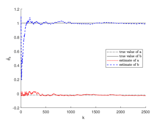
Then, the condition of Theorem 1 is satisfied. By the identification algorithm (4) with γ=3𝛾3\gamma=3, we can get the estimates of the parameters. Fig. 1 shows that the estimate θ^ksubscript^𝜃𝑘\hat{\theta}_{k} converges to the true parameter [0.02,1]Tsuperscript0.021𝑇[-0.02,1]^{T}, which is consistent with Theorem 1.

Refer to caption
Figure 1: Trajectories of estimates

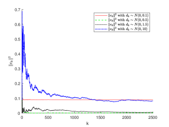
Let θ^0=[0,0.7]Tsubscript^𝜃0superscript00.7𝑇\hat{\theta}_{0}=[0,0.7]^{T}. The trajectories of the square of estimation error ek2superscriptnormsubscript𝑒𝑘2\|e_{k}\|^{2} with different variances of noise are given in Fig. 2, which shows that too small noise variance will affect the convergence, and too large noise variance will affect the convergence rate (fm,fMsubscript𝑓𝑚subscript𝑓𝑀f_{m},f_{M} are affected).

(2) Convergence rate of the estimation error

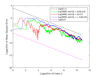
Fig. 3 shows the logarithm of the parameter estimation error vs the logarithm of the index k𝑘k with different initial estimates. From Fig. 3, we can see that the logarithms of the parameter estimation error with different initial estimates are all bounded by two linear functions of log(k)𝑘\log(k), which implies that the convergence rate of ekTeksuperscriptsubscript𝑒𝑘𝑇subscript𝑒𝑘e_{k}^{T}e_{k} is O(1/k)𝑂1𝑘O(1/k) and the initial estimates has almost no effect on the convergence rate. These results are consistent with Theorem 2.
Refer to caption
Figure 2: Trajectories of ek2superscriptnormsubscript𝑒𝑘2\|e_{k}\|^{2} with different variances of noise
Refer to caption
Figure 3: Trajectories of Log(MSE) with different θ^0subscript^𝜃0\hat{\theta}_{0}
Refer to caption
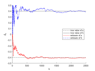
Figure 4: Trajectories of estimates with u=5𝑢5u=5

5.2 The case with [a,b]T=[0.4,0.4]Tsuperscript𝑎𝑏𝑇superscript0.40.4𝑇[a,b]^{T}=[-0.4,0.4]^{T}

The conclusion of our theorem is sufficient but not necessary. Consider another system with parameters θ=[a,b]T=[0.4,0.4]T𝜃superscript𝑎𝑏𝑇superscript0.40.4𝑇\theta=[a,b]^{T}=[-0.4,0.4]^{T} and the inputs uk=5subscript𝑢𝑘5u_{k}=5 as k𝑘k is odd and uk=0subscript𝑢𝑘0u_{k}=0 as k𝑘k is even. Let γ=2𝛾2\gamma=2, θ^0=[0.5,0.25]Tsubscript^𝜃0superscript0.50.25𝑇\hat{\theta}_{0}=[-0.5,0.25]^{T}. Obviously, the condition is not satisfied at this time. However, Fig. 4 shows the trajectories of the estimates θ^ksubscript^𝜃𝑘\hat{\theta}_{k} that can achieve to the true parameter.

6 Conclusions

This paper studies the identification of high-dimensional ARMA models with binary-valued observations. An online identification algorithm is proposed, which consists of parameter estimation and prediction of the original output. It is proved that the estimates can achieve the true parameter in mean square sense. The convergence rate of the proposed identification algorithm for high-dimensional ARMA models can achieve as the same convergence rate O(1/k) as the algorithm in Wang et al. (2021) for FIR models.

There are many meaningful future works. If the variance of noise is unknown, it can be estimated along with the parameters (see Wang et al. (2006)) by the proposed algorithm in this paper. It is worth studying whether the estimates still have good properties. Besides, the identification of ARMA models with multi-threshold quantized observations and the relationship between convergence rate and quantization level can be studied by referring to Guo and Zhao (2014). What’s more, there are some other interesting problems. For examples, how to construct an optimal identification algorithm in the sense of CR lower bound? How to apply the proposed algorithm to adaptive tracking control of systems with binary-valued observations?

Appendix

Appendix A Proof of Lemma 3

Proof 3.

The first equation in (5) is about wksubscript𝑤𝑘w_{k}, we first consider this type (replaced by wk1subscript𝑤𝑘1w_{k-1}):

{vk=(1αk)vk1+βkwk1+O(1k2),wk=awk1+vk1,\left\{\begin{aligned} v_{k}&=\left(1-\dfrac{\alpha}{k}\right)v_{k-1}+\dfrac{\beta}{k}w_{k-1}+O\left(\dfrac{1}{k^{2}}\right),\\ w_{k}&=aw_{k-1}+v_{k-1},\end{aligned}\right. (20)

where a,β>0𝑎𝛽0a,\beta>0. Obviously, first we make a<1,α>0formulae-sequence𝑎1𝛼0a<1,\alpha>0, otherwise it will not converge.

Let Ak=(1αkβk1a)subscript𝐴𝑘matrix1𝛼𝑘𝛽𝑘1𝑎A_{k}=\begin{pmatrix}1-\dfrac{\alpha}{k}&\dfrac{\beta}{k}\\ 1&a\end{pmatrix}, Bksubscript𝐵𝑘B_{k}=(O(1k2),0)Tsuperscriptmatrix𝑂1superscript𝑘20𝑇\begin{pmatrix}O\left(\dfrac{1}{k^{2}}\right),0\end{pmatrix}^{T} and Zk=(vk,wk)subscript𝑍𝑘superscriptmatrixsubscript𝑣𝑘subscript𝑤𝑘Z_{k}=\begin{pmatrix}v_{k},w_{k}\end{pmatrix}^{\prime}. Then (20) can be written as

Zk=AkZk1+Bk==AkA1Z0+l=1ki=l+1kAiBl.subscript𝑍𝑘subscript𝐴𝑘subscript𝑍𝑘1subscript𝐵𝑘subscript𝐴𝑘subscript𝐴1subscript𝑍0superscriptsubscript𝑙1𝑘superscriptsubscriptproduct𝑖𝑙1𝑘subscript𝐴𝑖subscript𝐵𝑙Z_{k}=A_{k}Z_{k-1}+B_{k}=\cdots=A_{k}\cdots A_{1}Z_{0}+\sum\limits_{l=1}^{k}\prod\limits_{i=l+1}^{k}A_{i}B_{l}.

We first calculate the eigenvalues λ1(k),λ2(k)subscript𝜆1𝑘subscript𝜆2𝑘\lambda_{1}(k),\lambda_{2}(k)and the corresponding eigenvectors p1(k),p2(k)subscript𝑝1𝑘subscript𝑝2𝑘p_{1}(k),p_{2}(k) of Aksubscript𝐴𝑘A_{k},

λ1(k)=1αaαβk(1a)+β[α(a1)+β]k2(a1)3+O(1k3)subscript𝜆1𝑘1𝛼𝑎𝛼𝛽𝑘1𝑎𝛽delimited-[]𝛼𝑎1𝛽superscript𝑘2superscript𝑎13𝑂1superscript𝑘3\lambda_{1}(k)=1-\dfrac{\alpha-a\alpha-\beta}{k(1-a)}+\dfrac{\beta[\alpha(a-1)+\beta]}{k^{2}(a-1)^{3}}+O\left(\dfrac{1}{k^{3}}\right)

λ2(k)=aβk(1a)β[α(a1)+β]k2(a1)3+O(1k3).subscript𝜆2𝑘𝑎𝛽𝑘1𝑎𝛽delimited-[]𝛼𝑎1𝛽superscript𝑘2superscript𝑎13𝑂1superscript𝑘3\lambda_{2}(k)=a-\dfrac{\beta}{k(1-a)}-\dfrac{\beta[\alpha(a-1)+\beta]}{k^{2}(a-1)^{3}}+O\left(\dfrac{1}{k^{3}}\right).

p1(k)=(111a+α(a1)+βk(a1)3+O(1k2)),subscript𝑝1𝑘matrix111𝑎𝛼𝑎1𝛽𝑘superscript𝑎13𝑂1superscript𝑘2p_{1}(k)=\begin{pmatrix}1\\ \dfrac{1}{1-a}+\dfrac{\alpha(a-1)+\beta}{k(a-1)^{3}}+O\left(\dfrac{1}{k^{2}}\right)\end{pmatrix},

p2(k)=(βk(a1)β[α(a1)+β]k2(a1)3+O(1k3)1).subscript𝑝2𝑘matrix𝛽𝑘𝑎1𝛽delimited-[]𝛼𝑎1𝛽superscript𝑘2superscript𝑎13𝑂1superscript𝑘31p_{2}(k)=\begin{pmatrix}\dfrac{\beta}{k(a-1)}-\dfrac{\beta[\alpha(a-1)+\beta]}{k^{2}(a-1)^{3}}+O\left(\dfrac{1}{k^{3}}\right)\\ 1\end{pmatrix}.

Hence we get the characteristic matrix Pksubscript𝑃𝑘P_{k} and its inverse,

Pk=(1βk(a1)β[α(a1)+β]k2(a1)3+O(1k3)11a+α(a1)+βk(a1)3+O(1k2)1),subscript𝑃𝑘1𝛽𝑘𝑎1limit-from𝛽delimited-[]𝛼𝑎1𝛽superscript𝑘2superscript𝑎13𝑂1superscript𝑘311𝑎𝛼𝑎1𝛽𝑘superscript𝑎13𝑂1superscript𝑘21P_{k}=\left(\begin{aligned} 1\quad\quad\dfrac{\beta}{k(a-1)}-\dfrac{\beta[\alpha(a-1)+\beta]}{k^{2}(a-1)^{3}}+&O\left(\dfrac{1}{k^{3}}\right)\\ \dfrac{1}{1-a}+\dfrac{\alpha(a-1)+\beta}{k(a-1)^{3}}+O\left(\dfrac{1}{k^{2}}\right)&\quad\quad 1\end{aligned}\right),

Pk1=(pk11,pk12pk21,pk22)superscriptsubscript𝑃𝑘1matrixsuperscriptsubscript𝑝𝑘11superscriptsubscript𝑝𝑘12superscriptsubscript𝑝𝑘21superscriptsubscript𝑝𝑘22P_{k}^{-1}=\begin{pmatrix}p_{k}^{11},p_{k}^{12}\\ p_{k}^{21},p_{k}^{22}\end{pmatrix}, where

pk11=1βk(1a)2+3β2+2βα(a1)k2(1a)4+O(1k3)superscriptsubscript𝑝𝑘111𝛽𝑘superscript1𝑎23superscript𝛽22𝛽𝛼𝑎1superscript𝑘2superscript1𝑎4𝑂1superscript𝑘3p_{k}^{11}=1-\dfrac{\beta}{k(1-a)^{2}}+\dfrac{3\beta^{2}+2\beta\alpha(a-1)}{k^{2}(1-a)^{4}}+O\left(\dfrac{1}{k^{3}}\right),

pk12=βk(1a)+β[α(a1)+2β]k2(a1)3+O(1k3)superscriptsubscript𝑝𝑘12𝛽𝑘1𝑎𝛽delimited-[]𝛼𝑎12𝛽superscript𝑘2superscript𝑎13𝑂1superscript𝑘3p_{k}^{12}=\dfrac{\beta}{k(1-a)}+\dfrac{\beta[\alpha(a-1)+2\beta]}{k^{2}(a-1)^{3}}+O\left(\dfrac{1}{k^{3}}\right),

pk21=1a1+α(a1)+2βk(1a)3+O(1k2)superscriptsubscript𝑝𝑘211𝑎1𝛼𝑎12𝛽𝑘superscript1𝑎3𝑂1superscript𝑘2p_{k}^{21}=\dfrac{1}{a-1}+\dfrac{\alpha(a-1)+2\beta}{k(1-a)^{3}}+O\left(\dfrac{1}{k^{2}}\right),

pk22=1βk(1a)2+3β2+2βα(a1)k2(1a)4+O(1k3)superscriptsubscript𝑝𝑘221𝛽𝑘superscript1𝑎23superscript𝛽22𝛽𝛼𝑎1superscript𝑘2superscript1𝑎4𝑂1superscript𝑘3p_{k}^{22}=1-\dfrac{\beta}{k(1-a)^{2}}+\dfrac{3\beta^{2}+2\beta\alpha(a-1)}{k^{2}(1-a)^{4}}+O\left(\dfrac{1}{k^{3}}\right).

Let η=α+βa1𝜂𝛼𝛽𝑎1\eta=\alpha+\dfrac{\beta}{a-1}, and since Ak=Pk(λ1(k)00λ2(k))Pk1subscript𝐴𝑘subscript𝑃𝑘matrixsubscript𝜆1𝑘00subscript𝜆2𝑘superscriptsubscript𝑃𝑘1A_{k}=P_{k}\begin{pmatrix}\lambda_{1}(k)&0\\ 0&\lambda_{2}(k)\end{pmatrix}P_{k}^{-1}, we have

AkA1=i=1kPi(λ1(i)00λ2(i))Pi1=Pk{i=2k(λ1(i)00λ2(i))Pi1Pi1}(λ1(1)00λ2(1))P11.missing-subexpressionsubscript𝐴𝑘subscript𝐴1superscriptsubscriptproduct𝑖1𝑘subscript𝑃𝑖matrixsubscript𝜆1𝑖00subscript𝜆2𝑖superscriptsubscript𝑃𝑖1missing-subexpressionabsentsubscript𝑃𝑘superscriptsubscriptproduct𝑖2𝑘matrixsubscript𝜆1𝑖00subscript𝜆2𝑖superscriptsubscript𝑃𝑖1subscript𝑃𝑖1matrixsubscript𝜆1100subscript𝜆21superscriptsubscript𝑃11\begin{aligned} &\quad A_{k}\cdots A_{1}=\prod\limits_{i=1}^{k}P_{i}\begin{pmatrix}\lambda_{1}(i)&0\\ 0&\lambda_{2}(i)\end{pmatrix}P_{i}^{-1}\\ &=P_{k}\left\{\prod\limits_{i=2}^{k}\begin{pmatrix}\lambda_{1}(i)&0\\ 0&\lambda_{2}(i)\end{pmatrix}P_{i}^{-1}P_{i-1}\right\}\begin{pmatrix}\lambda_{1}(1)&0\\ 0&\lambda_{2}(1)\end{pmatrix}P_{1}^{-1}.\end{aligned}

Consider

(λ1(k)00λ2(k))Pk1Pk1matrixsubscript𝜆1𝑘00subscript𝜆2𝑘superscriptsubscript𝑃𝑘1subscript𝑃𝑘1\displaystyle\begin{pmatrix}\lambda_{1}(k)&0\\ 0&\lambda_{2}(k)\end{pmatrix}P_{k}^{-1}P_{k-1}
=\displaystyle= (1ηk+O(1k2)O(1k2)O(1k2)a+1k(βa1)+O(1k2)),matrix1𝜂𝑘𝑂1superscript𝑘2𝑂1superscript𝑘2𝑂1superscript𝑘2𝑎1𝑘𝛽𝑎1𝑂1superscript𝑘2\displaystyle\begin{pmatrix}1-\dfrac{\eta}{k}+O\left(\dfrac{1}{k^{2}}\right)&O\left(\dfrac{1}{k^{2}}\right)\\ O\left(\dfrac{1}{k^{2}}\right)&a+\dfrac{1}{k}(\dfrac{\beta}{a-1})+O\left(\dfrac{1}{k^{2}}\right)\end{pmatrix},

and

i=2ksuperscriptsubscriptproduct𝑖2𝑘\displaystyle\prod\limits_{i=2}^{k} (1ηk+O(1k2))=ei=2kln(1ηi+O(1k2))1𝜂𝑘𝑂1superscript𝑘2superscript𝑒superscriptsubscript𝑖2𝑘1𝜂𝑖𝑂1superscript𝑘2\displaystyle\left(1-\dfrac{\eta}{k}+O\left(\dfrac{1}{k^{2}}\right)\right)=e^{\sum\limits_{i=2}^{k}\ln\left(1-\dfrac{\eta}{i}+O\left(\dfrac{1}{k^{2}}\right)\right)}
=\displaystyle= ei=2kηi+O(1i2)=eηlnk+C1=C2kη.superscript𝑒superscriptsubscript𝑖2𝑘𝜂𝑖𝑂1superscript𝑖2superscript𝑒𝜂𝑘subscript𝐶1subscript𝐶2superscript𝑘𝜂\displaystyle e^{-\sum\limits_{i=2}^{k}\dfrac{\eta}{i}+O\left(\dfrac{1}{i^{2}}\right)}=e^{-\eta\ln k+C_{1}}=C_{2}k^{-\eta}.

Then i=2k(λ1(i)00λ2(i))Pi1Pi1=O(1kη),superscriptsubscriptproduct𝑖2𝑘matrixsubscript𝜆1𝑖00subscript𝜆2𝑖superscriptsubscript𝑃𝑖1subscript𝑃𝑖1𝑂1superscript𝑘𝜂\prod\limits_{i=2}^{k}\begin{pmatrix}\lambda_{1}(i)&0\\ 0&\lambda_{2}(i)\end{pmatrix}P_{i}^{-1}P_{i-1}=O\left(\dfrac{1}{k^{\eta}}\right), and AkA1=O(1kη)subscript𝐴𝑘subscript𝐴1𝑂1superscript𝑘𝜂A_{k}\cdots A_{1}=O\left(\dfrac{1}{k^{\eta}}\right) for η>0𝜂0\eta>0, otherwise it will not converge. Similarly, we can get i=lkAi=O((lk)η)superscriptsubscriptproduct𝑖𝑙𝑘subscript𝐴𝑖𝑂superscript𝑙𝑘𝜂\prod\limits_{i=l}^{k}A_{i}=O\left(\left(\dfrac{l}{k}\right)^{\eta}\right).

Then

l=1kBli=l+1kAi=l=1kO((l+1k)η)O(1l2)superscriptsubscript𝑙1𝑘subscript𝐵𝑙superscriptsubscriptproduct𝑖𝑙1𝑘subscript𝐴𝑖superscriptsubscript𝑙1𝑘𝑂superscript𝑙1𝑘𝜂𝑂1superscript𝑙2\displaystyle\sum\limits_{l=1}^{k}B_{l}\prod\limits_{i=l+1}^{k}A_{i}=\sum\limits_{l=1}^{k}O\left((\dfrac{l+1}{k})^{\eta}\right)O\left(\dfrac{1}{l^{2}}\right)
=\displaystyle= O(l=1k(l+1)η2kη)={O(1k),η1;O(lnkk),η=1.\displaystyle O\left(\sum\limits_{l=1}^{k}\dfrac{(l+1)^{\eta-2}}{k^{\eta}}\right)=\left\{\begin{aligned} &O\left(\dfrac{1}{k}\right),&\eta\neq 1;\\ &O\left(\dfrac{lnk}{k}\right),&\eta=1.\end{aligned}\right.

Hence for any Z0=(v0,w0)Tsubscript𝑍0superscriptsubscript𝑣0subscript𝑤0𝑇Z_{0}=(v_{0},w_{0})^{T} and

Zk=AkA1Z0+l=1ki=l+1kAiBl={O(1kη),0<η<1;O(lnkk),η=1;O(1k),η>1.Z_{k}=A_{k}\cdots A_{1}Z_{0}+\sum\limits_{l=1}^{k}\prod\limits_{i=l+1}^{k}A_{i}B_{l}\\ =\left\{\begin{aligned} &O(\dfrac{1}{k^{\eta}}),&0<\eta<1;\\ &O(\dfrac{lnk}{k}),&\eta=1;\\ &O(\dfrac{1}{k}),&\eta>1.\end{aligned}\right.

Considering (5) and substituting the second formula into the first, we have

{vk=(1αβk)vk1+aβkwk1+O(1k2),wk=awk1+vk1.\left\{\begin{aligned} v_{k}&=\left(1-\dfrac{\alpha-\beta}{k}\right)v_{k-1}+\dfrac{a\beta}{k}w_{k-1}+O\left(\dfrac{1}{k^{2}}\right),\\ w_{k}&=aw_{k-1}+v_{k-1}.\end{aligned}\right.

According to the above discussion, the conditions to be met are 0<a<1,αβ>0formulae-sequence0𝑎1𝛼𝛽00<a<1,\alpha-\beta>0, and η=α+βa1>0𝜂𝛼𝛽𝑎10\eta=\alpha+\dfrac{\beta}{a-1}>0.

To sum up, The vector (vk,wk)Tsuperscriptsubscript𝑣𝑘subscript𝑤𝑘𝑇(v_{k},w_{k})^{T} converges to zero if and only if η>0𝜂0\eta>0 and α>0𝛼0\alpha>0. And, the convergence rate can be obtained.

Appendix B Proof of Lemma 4

Proof 4.

i) If xn++xn+N1N=O(1nt),subscript𝑥𝑛subscript𝑥𝑛𝑁1𝑁𝑂1superscript𝑛𝑡\dfrac{x_{n}+\cdots+x_{n+N-1}}{N}=O\left(\dfrac{1}{n^{t}}\right), then

0xnNxn++xn+N1N=O(1nt)0subscript𝑥𝑛𝑁subscript𝑥𝑛subscript𝑥𝑛𝑁1𝑁𝑂1superscript𝑛𝑡0\leq\dfrac{x_{n}}{N}\leq\dfrac{x_{n}+\cdots+x_{n+N-1}}{N}=O\left(\dfrac{1}{n^{t}}\right)

xn=O(1nt).absentsubscript𝑥𝑛𝑂1superscript𝑛𝑡\Rightarrow x_{n}=O\left(\dfrac{1}{n^{t}}\right).

ii) If xn=O(1nt),subscript𝑥𝑛𝑂1superscript𝑛𝑡x_{n}=O\left(\dfrac{1}{n^{t}}\right), then xn+l=O(1(n+l)t)=O(1nt),l=1,,N1.formulae-sequencesubscript𝑥𝑛𝑙𝑂1superscript𝑛𝑙𝑡𝑂1superscript𝑛𝑡𝑙1𝑁1x_{n+l}=O\left(\dfrac{1}{(n+l)^{t}}\right)=O\left(\dfrac{1}{n^{t}}\right),l=1,\ldots,N-1. Hence xn++xn+N1N=O(1nt).subscript𝑥𝑛subscript𝑥𝑛𝑁1𝑁𝑂1superscript𝑛𝑡\dfrac{x_{n}+\cdots+x_{n+N-1}}{N}=O\left(\dfrac{1}{n^{t}}\right). The lemma is proved.

References

  • Bi et al. (2015) Wenjian Bi, Guolian Kang, Yanlong Zhao, et al. SVSI: Fast and powerful set-valued system identification approach to identifying rare variants in sequencing studies for ordered categorical traits. Annals of human genetics, 79(4):294–309, 2015.
  • Bradfield et al. (2012) Jonathan P. Bradfield, H. Rob Taal, Nicholas J. Timpson, et al. A genome-wide association meta-analysis identifies new childhood obesity loci. Nature genetics, 44(5):526, 2012.
  • Calamai and Moré (1987) Paul H. Calamai and Jorge J. Moré. Projected gradient methods for linearly constrained problems. Mathematical programming, 39(1):93–116, 1987.
  • Casini et al. (2007) Marco Casini, Andrea Garulli, and Antonio Vicino. Time complexity and input design in worst-case identification using binary sensors. In 46th IEEE Conference on Decision and Control, pages 5528–5533, 2007.
  • Chen and Guo (1987) Han-Fu Chen and Lei Guo. Adaptive control via consistent estimation for deterministic systems. International Journal of Control, 45(6):2183–2202, 1987.
  • Godoy et al. (2011) Boris I. Godoy, Graham C. Goodwin, Juan C. Agüero, Damián Marelli, and Torbjörn Wigren. On identification of FIR systems having quantized output data. Automatica, 47(9):1905–1915, 2011.
  • Guo and Zhao (2013) Jin Guo and Yanlong Zhao. Recursive projection algorithm on FIR system identification with binary-valued observations. Automatica, 49(11):3396–3401, 2013.
  • Guo and Zhao (2014) Jin Guo and Yanlong Zhao. Identification of the gain system with quantized observations and bounded persistent excitations. Science China Information Sciences, 57(012205):1–15, 2014.
  • Marelli et al. (2013) Damián Marelli, Keyou You, and Minyue Fu. Identification of ARMA models using intermittent and quantized output observations. Automatica, 49(2):360–369, 2013.
  • Wang et al. (2002) Le Yi Wang, Yong-Wha Kim, and Jing Sun. Prediction of oxygen storage capacity and stored NOx by HEGO sensors for improved LNT control strategies. In ASME International Mechanical Engineering Congress and Exposition, 777–785, 2002.
  • Wang et al. (2003) Le Yi Wang, Ji-Feng Zhang, and G. George Yin. System identification using binary sensors. IEEE transactions on automatic control, 48(11):1892–1907, 2003.
  • Wang et al. (2006) Le Yi Wang, G. George Yin, and Ji-Feng Zhang. Joint identification of plant rational models and noise distribution functions using binary-valued observations. Automatica, 42:535–547, 2006.
  • Wang et al. (2010) Le Yi Wang, G. George Yin, Ji-Feng Zhang, and Yanlong Zhao. System identification with quantized observations. Springer, 2010.
  • Wang et al. (2016) Ting Wang, Wenjian Bi, Yanlong Zhao, and Wenchao Xue. Radar target recognition algorithm based on RCS observation sequence – set-valued identification method. Journal of Systems Science and Complexity, 29(3):573–588, 2016.
  • Wang et al. (2018) Ting Wang, Jianwei Tan, and Yanlong Zhao. Asymptotically efficient non-truncated identification for FIR systems with binary-valued outputs. Science China Information Sciences, 61(12):129208, 2018.
  • Wang et al. (2021) Ting Wang, Min Hu, and Yanlong Zhao. Adaptive tracking control of FIR systems under binary-valued observations and recursive projection identification. IEEE Transactions on Systems, Man, and Cybernetics: Systems, 51(9):5289–5299, 2021.
  • Woodward et al. (2017) Wayne A Woodward, Henry L Gray, and Alan C Elliott. Applied time series analysis with R. CRC press, 2017.
  • You (2015) Keyou You. Recursive algorithms for parameter estimation with adaptive quantizer. Automatica, 52:192–201, 2015.
  • Yu et al. (2016) Chengpu Yu, Keyou You, and Lihua Xie. Quantized identification of ARMA systems with colored measurement noise. Automatica, 66:101–108, 2016.
  • Isaacson, et al. (1994) Eugene Isaacson, & Herbert Bishop Keller (1994). Analysis of numerical methods. Courier Corporation.
  • Zhang et al. (2019) Hang Zhang, Ting Wang, and Yanlong Zhao. FIR system identification with set-valued and precise observations from multiple sensors. Science China Information Sciences, 62(5):52203, 2019.
  • Zhang et al. (2021) Hang Zhang, Ting Wang, and Yanlong Zhao. Asymptotically efficient recursive identification of FIR systems with binary-valued observations. IEEE Transactions on Systems, Man, and Cybernetics: Systems, 51(5):2687–2700, 2021.
  • Zhao et al. (2016) Yanlong Zhao, Wenjian Bi, and Ting Wang. Iterative parameter estimate with batched binary-valued observations. Science China Information Sciences, 59(5):052201, 2016.
  • Wang et al. (2023) Ting Wang, Xin Li, Jin Guo, and Yanlong Zhao. Identification of ARMA models with binary-valued observations. Automatica, 149, 110832, 2023.