Propensity Score Alignment of Unpaired Multimodal Data
Abstract
Multimodal representation learning techniques typically rely on paired samples to learn common representations, but paired samples are challenging to collect in fields such as biology where measurement devices often destroy the samples. This paper presents an approach to address the challenge of aligning unpaired samples across disparate modalities in multimodal representation learning. We draw an analogy between potential outcomes in causal inference and potential views in multimodal observations, which allows us to use Rubin’s framework to estimate a common space in which to match samples. Our approach assumes we collect samples that are experimentally perturbed by treatments, and uses this to estimate a propensity score from each modality, which encapsulates all shared information between a latent state and treatment and can be used to define a distance between samples. We experiment with two alignment techniques that leverage this distance—shared nearest neighbours (SNN) and optimal transport (OT) matching—and find that OT matching results in significant improvements over state-of-the-art alignment approaches in both a synthetic multi-modal setting and in real-world data from NeurIPS Multimodal Single-Cell Integration Challenge.
1 Introduction
Large-scale multimodal representation learning techniques such as CLIP (Radford et al., 2021) have lead to remarkable improvements in zero-shot classification performance and have enabled the recent success in conditional generative models. However, the effectiveness of multimodal methods hinges on the availability of paired samples—such as images and their associated captions—across data modalities. This reliance on paired samples is most obvious in the InfoNCE loss (Gutmann & Hyvärinen, 2010; van den Oord et al., 2018) used in CLIP (Radford et al., 2021) which explicitly learns representations to maximize the true matching between images and their captions.
While paired image captioning data is abundant on the internet, paired multimodal data is often challenging to collect in scientific experiments. Take, for instance, experiments in biology, where unpaired data are the norm for technical reasons: RNA sequencing, protein expression assays, and the collection of microscopy images for cell painting experimental assays are all destructive processes. Because of this, we cannot collect multiple different measurements from the same cell, and can only explicitly group cells by their experimental condition.
If we could accurately match unpaired samples across modalities, we could use the aligned samples as proxies for paired samples and apply existing multimodal representation learning techniques. However, matching across modalities is challenging for two reasons. Firstly, observations from various modalities often exist in entirely different spaces. For instance, microscopy images of cells are in pixel space, while gene expression assays provide data in the form of mRNA abundance counts. Secondly, even if measurements were taken in the same space, determining an appropriate distance metric for matching remains a non-trivial task. For example, when matching images of distinct cells in different microscopy images, we would ideally want a metric that is more sensitive to features describing the underlying state of the cell than features related to biologically-irrelevant cell appearance, such as the orientation of the cell.
To understand the matching problem more abstractly, we can think of the multiple modalities as potential “views”, of the same underlying latent state, , where we only get to observe one view for any individual unit (e.g. an individual cell in our motivating example). Observing, or accurately inferring would address the first issue by providing a common space in we could match samples. However, inferring the latent variable is hopelessly underspecified without making strong assumptions on the data generating processes of both modalities (Xi & Bloem-Reddy, 2023). Furthermore, for complex systems such as biological samples, may still be extremely high-dimensional, and as a result, the second challenge remains: what is the “right” metric is for measuring similarity between samples in this space?
We address both challenges in this paper by appealing to classical ideas from Rubin (1974), in the case where we additionally observe a label for each unit , e.g., indexing an experiment that it belongs to. By making the assumption that perturbs the observations via their shared latent state, we identify an observable link between modalities with the same underlying . Our key observation is that the propensity score, defined as , satisfies three properties: 1) It provides a common space for matching, 2) it maximally coarsens , retaining only relevant information and 3) under certain assumptions, it is estimable from observations of individual modalities alone (Proposition 3.1).
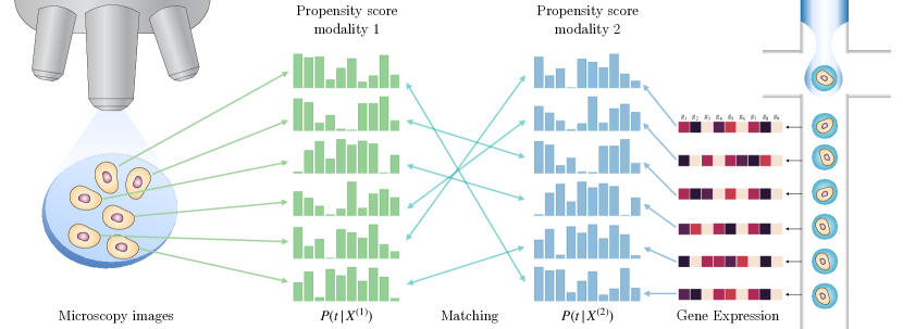
In practice, the propensity score is straightforward to estimate: one simply trains two classifiers—one for each modality—to predict which treatment was applied to the respective modalities, and then match across modalities based on the similarity between predicted treatments within each treatment group. The proposed methodology is generic across modalities—it can be applied to match observations between any modality for which a classifier can be efficiently trained. However, we cannot naively use bipartite matching, as the same sample unit does not appear in both modalities. To address this, we use soft matching techniques to estimate the missing modality for each sample unit by combining multiple observations. We experiment with two different matching approaches from the recent literature: shared nearest neighbours (SNN) matching (Lance et al., 2022; Cao & Gao, 2022) and optimal transport (OT) matching Villani (2009); Schiebinger et al. (2019), and find that OT matching with distances defined on the propensity score lead to significant improvement on real world multi-modal matching tasks from the NeurIPS Multimodal Single-Cell Integration Challenge Lance et al. (2022). We found similarly large improvements on synthetic image-based benchmarks.
Finally, we show how our matching procedure can be used for cross-modality prediction tasks. We estimate a function that translates between modalities by integrating over the coupling matrix output by our alignment procedure. Our approach uses a two-sample stochastic gradient estimator to get an unbiased estimate of the gradient of the resulting loss. In our experiments, this approach gave very strong performance, even outperforming methods that had access to the ground truth matching.
2 Related work
Unpaired Data Dealing with unpaired data is important in translation tasks, either for images (Liu et al., 2017; Zhu et al., 2017; Almahairi et al., 2018), or more recently for biological modalities (Amodio & Krishnaswamy, 2018; Yang et al., 2021). In particular, Yang et al. (2021) formalize this setting as being generated by a shared underlying latent variable, which has also been identified as a useful modelling assumption for identifiability analyses in multi-view or multi-modal representation learning (Gresele et al., 2020; Sturma et al., 2023). Our work also exploits this modelling assumption for theoretical justification, but, unlike previous works, our method does not depend on performing inference over the latent space, thus avoiding the identifiability issue. Specifically, since we do not require modality translation, we do not require an encoder-decoder structure (Yang et al., 2021), which embeds modality-specific reconstruction information in the latent space that can be detrimental for the simpler matching task.
Optimal Transport Matching Optimal transport is commonly used to solve a similar problem in single-cell biology known as cell trajectory inference. In this case, to are random variables measured at different time points in a shared (metric) space, and OT matching can be achieved by minimizing the metric (Schiebinger et al., 2019; Tong et al., 2020). Recent work (Demetci et al., 2022) tackles our multi-modal alignment problem by using the Gromov-Wasserstein distance, which leverages local metric structure within pairs of points from each modality (Demetci et al., 2022). In addition to this “pure” OT approach, Gossi et al. (2023) use OT on contrastive learning representations, though this approach requires matched pairs for training, while Cao et al. (2022) use OT in the latent space of a multi-modal VAE.
Perturbations and Heterogeneity Many methods treat observation-level heterogeneity as another dimension to globally integrate, even when cluster labels are observed (Butler et al., 2018; Korsunsky et al., 2019; Foster et al., 2022). This is sensible when clusters correspond to noise rather than the signal of interest. However, it is well known in causal representation learning that heterogeneity—particularly heterogeneity arising from different perturbations—has theoretical benefits (Khemakhem et al., 2020; Squires et al., 2023; Ahuja et al., 2023; Buchholz et al., 2023; von Kügelgen et al., 2023). There, the benefits (weakly) increase with the number of perturbations, which is also true of our setting (Proposition 3.2). In the context of aligning unpaired data, only Yang et al. (2021) leverage this heterogeneity in their method. Specifically, they require VAE representations to classify experimental labels in addition to reconstructing modalities, while our method only requires a representation to classify labels. Yang et al. (2021) treat the classifier objective as a regularizer, but our theory suggests that it is responsible for their matching performance. In our experiments, we found that requiring reconstruction led to worse matching performance with equivalent architectures.
3 Propensity Score Multi-modal Matching
We consider multimodal settings where there exist two potential views, from two different modalities indexed by and experiment that perturbs a shared latent state of these observations. The observations will typically be in very different spaces: for example, may be the space of images of cells under a microscope, and may be the space of gene expression data. This process defines a jointly distributed random variable , from which we observe only a single modality, its index, and treatment assignment, (we will always denote random variables by upper-case letters, and samples by their corresponding lower-case letter). Our aim is to match or estimate the samples from the missing modality that would correspond to the realization of the missing random variable. Importantly, we match within treatment groups, and the treatment variable is only used to learn a common space in which to match.
We assume each modality arises from a common latent random variable as follows,
| (1) |
where indexes the experimental perturbations, ensures that has a non-trivial affect on the distribution of the latent variables, and we can take to represent a base environment. Note that the structural equations are deterministic after accounting for the randomness in and : it represents purely the measurement process that captures the latent state. For example, in a microscopy image, this would be the microscope and camera that maps a cell to pixels. The modality specific noise variables, , play the role of measurement noise and modality-specific factors of variation: e.g. , could describe the layout and orientation of cells on a slide.
Under this model, if were observable, an optimal matching can be constructed by simply matching the modalities with the most similar . However, is latent, and inference on the model described by Section 3 is arguably more difficult than the matching problem itself due to theoretical difficulties such as identifiability and disentangling from the modality-specific noise terms .
Instead, we see that the interventions provide an observable link between the modalities, thereby revealing information about . Specifically, we use the propensity score with respect to , which we define as
| (2) |
as a proxy for the latent . Now, although we cannot compute this directly as is latent, we make the observation that if is injective for , then we can compute the compute the propensity score from each of the observed modalities, since it will be that , for both and . Not only does the propensity score reveal shared information, classical causal inference (Rubin, 1974) states that it captures all information shared between the latent and treatment, and does so minimally, in terms of having minimum dimension and entropy. We collect these observations into the following proposition.
Proposition 3.1.
In the model described by Section 3, further assume that are injective for . Then, the propensity score in either modality is equal to the propensity score given by , i.e., as random variables. This implies
| (3) |
for each , where is the mutual information. Furthermore, any other function satisfying is such that .
The proof can be found in the Appendix. The above shows that computing the propensity score on either modality is equivalent to computing it on the unobserved shared latent, which captures all the shared information observable in . The final statement implies that it is of minimal dimension and entropy, and thus it discards the modality-specific information that may be counterproductive to matching.
Number of Perturbations Note that point-wise equality of the propensity score does not necessarily imply equality of the latents , due to potential non-injectivity. In fact, suppose that is supported in . The propensity score maps into the -dimensional simplex, where is the number of perturbations, which can be parameterized by coordinates in (essentially, the logits of the classifier). Under mild conditions, the propensity score necessarily compresses information about if the latent dimension exceeds the number of perturbations, echoing impossibility results from the causal representation learning literature (Squires et al., 2023).
Proposition 3.2.
Suppose that has a smooth density for each . Then, if , the propensity score , restricted to its strictly positive part, is non-injective.
The proof can be found in the Appendix. Note the above only states an impossibility result when . When , it can be seen from the proof of Proposition 3.2 that the injectivity of the propensity score depends on the injectivity of the following expression in :
| (4) |
which then depends on the latent process itself. If the above is non-injective, this is a fundamental indeterminacy that cannot be resolved without making strong assumptions on point-wise latent variable recovery, as we have already seen that the propensity score contains the maximal shared information, as shown in Proposition 3.1. Nonetheless, note that in Equation 4 is injective if any of the subset of its entries are, clearly outlining the benefits of collecting data from a larger number of perturbations for matching.
Key Assumptions Our results thus far rely on two key modelling assumptions,
-
•
(A1): has a non-trivial effect on , but does not affect , implying that interventions are able to target the common underlying process without changing modality-specific properties.
-
•
(A2): Injectivity of in the propensity score derivation, , which implies each modality contains complete information about the underlying process.
(A1) is justifiable insofar as modalities represent different measurements of an isolated system, such as in biological studies where might correspond to an underlying cell state and modalities refer to different single-cell measurements. However, in practice, even different measurement devices may be more or less sensitive to the biological variation implied by . We weaken this assumption in a simplified case in Section 3.
(A2) requires that no information about the latent state is lost in the observation process. Note that the injectivity is in the sense of as a function of both and , which allows observations that have a shared but differ by their value in , and the function remains injective. For example, rotated images with the exact same content can have a shared , but remain injective due to the rotation being captured in .
Relaxing Assumption 1
Consider the propensity score
| (5) |
where we do not necessarily require , and thus we obtain
| (6) | |||
see the proof of Proposition 3.1 for details.
Suppose that the two observed modalities are indeed generated by a shared , but where the indices of modality are potentially permuted, and with values differing by modality specific information:
| (7) |
where denotes a permutation of the sample indices. Under (A1), we would be able to find some such that for each .
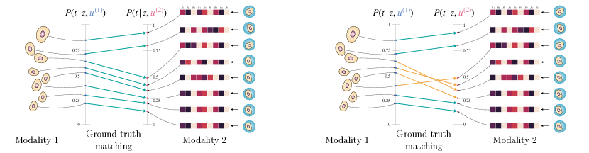
Matching via OT can allow us to relax (A1) in a very particular way. Consider the simple case where , so that can be written in a single dimension, e.g., . In this case, exact OT is equivalent to sorting and , and matching the sorted versions 1-to-1. Under (A1), the sorted versions will be exactly equal. A relaxed version of (A1) that would still result in the correct ground truth matching is to assume that affects and differently, but that the difference is order preserving, or monotone. Denote as the true pairing, noting that we use the same index . We require the following:
| (8) |
This says that, even if , that their relative orderings will still coincide. Then, exact OT will still recover the ground truth matching. See Figure 2 for a visual example of this type of monotonicity. For example, suppose that is a chemical perturbation of a cell, and thus , can be seen as a measure of biological response to the perturbation, e.g., in a treated population, indicates samples had a stronger response than sample , as perceived by the first modality indexed by . Then, this monotonocity states that we should see the same in the other modality as well, if the samples and truly corresponded to and .
When is not a binary treatment and the propensity scores are multidimensional, a condition known as cyclic monotonicity is sufficient for recovering the true matching, see Appendix A for details. However, unlike the 1-d case, we are not aware of more intuitive conditions under which we should expect cyclic monotonicity to hold.
4 Methodology
For the remainder, we will drop from our notation, and use to denote observations from modality 1, and to denote observations from modality 2 whenever it does not cause confusion to do so. Given a multimodal dataset with observations and , we wish to compute a matching matrix (or coupling) between the two modalities. We define a matching matrix where represents the likelihood of being matched to . We always perform matching only within observations with the same value of , so that in practice we obtain a matrix for each .
Our method approximates the propensity scores by training separate classifiers that predicts given for each modality. We denote the estimated propensity score by and respectively, where
| (9) |
This results in the transformed datasets and , where , are in the dimensional simplex. We use this correspondence to compute a cross-modality distance function:
| (10) |
where in practice, we typically compute the Euclidean distance in of the logit-transformed classification scores. Given this distance function, we rely on existing matching techniques to constructing a matching matrix. In our experiments, we found OT matching gave the best performance, but we also evaluated Shared Nearest Neighbour matching; details of the latter can be found in Appendix B.
4.1 Optimal Transport Matching
The propensity score distance allows us to easily compute a cost function associated with transporting mass between modalities, . Let denote the uniform distribution over and respectively. Discrete OT aims to solve the problem of optimally redistributing mass from to in terms of incurring the lowest cost. Let denote the cost matrix. The Kantorovich formulation of optimal transport aims to solve the following constrained optimization problem:
This is a linear program, and for , it can be shown that the optimal solution is a bipartite matching between and . We refer to this as exact OT; in practice we add an entropic regularization term, resulting in a soft matching, that ensures smoothness and uniqueness, and can be solved efficiently using Sinkhorn’s algorithm. Entropic OT takes the following form:
where , the entropy of the joint distribution implied by . This approach regularizes towards a higher entropy solution, which has been shown to have statistical benefits (Genevay et al., 2018), but nonetheless for small enough serves as a computationally appealing approximation to exact OT.
5 Cross-modality prediction
Given a matching matrix , we can interpret this as the probability that each sample, , from modality (1) is matched to sample in modality (2); that is . As a downstream task, and as an evaluation metric for , we can use this matching to estimate a cross-modal prediction model, , that maps from modality (2) to (1) by minimizing the following loss,
| (11) |
However, this requires evaluating for all examples from modality (2) for each of the examples in modality (1). Of course, we can avoid this cost with stochastic gradient descent by sampling from modality via for each training example , but to get an unbiased estimate of , we need two samples from modality (2) for each sample from modality (1),
| (12) |
By taking two samples as in equation (12), we get an unbiased estimator of , whereas a single sample would have resulted in optimizing an upper-bound on equation (11); for details, see Hartford et al. (2017) where a similar issue arises in the gradient of their causal effect estimator.
6 Experiments
We evaluate our proposed methodology on two datasets. The first is a synthetic interventional image dataset generated satisfying the assumptions of Section 3. The second is a real-world single-cell CITE-seq data obtained from the NeurIPS 2021 Multimodal single-cell data integration competition (Lance et al., 2022), which provides a ground truth matching by allowing for a small number of cell surface proteins to be measured simultaneously to RNA sequencing. Note the CITE-seq dataset is not interventional—we use the cell type as the classification target instead. All details are made available in the Appendix. In both cases the ground truth matching is known to make evaluation possible, but hidden during training.
Baselines In terms of the problem setting, the most closely related method is Gromov-Wasserstein optimal transport (SCOT) (Demetci et al., 2022), which explicitly computes a cross-modality cost for optimal transport matching by leveraging the local geometry within each modality. For the CITE-seq data, graph-linked VAE (scGLUE), which has access to specific biological metadata that connects the biological modalities, can also be used for matching.222A variant of scGLUE was the top entrant in the NeurIPS 2021 Multi-modal single-cell data integration competition, from which we source our data. However, ground truth matchings were made available in the training set in that case, which fundamentally changes the nature and difficulty of the problem. However, neither of the preceding approaches use the experimental label information, which is a key component of our method. In fact, the only method to our knowledge that leverages such information is the VAE approach developed in Yang et al. (2021), which also minimizes a classification loss from the latent space, which we will consider our main baseline. For all methods besides SCOT, we use both SNN and OT to perform the final matching in the latent space. Note that when combined with OT, our VAE baseline also resembles Cao et al. (2022).
Model Details For our method and the VAE, we use the general architecture of a linear classification head on top of a suitable encoder. The architecture of this encoder is always the same between the VAE and our method. For the image dataset, we use the convolutional neural network from Yang et al. (2021) as the encoder, and for the CITE-seq dataset, we use fully-connected MLPs for both RNA (top 200 PC’s) and protein data. Optimization was performed using Adam with a one-cycle learning rate scheduler. We use the standard cross-entropy loss to train our classifiers for propensity score estimation. For other methods, we use existing implementations with suggested default settings.
Matching Details Both SNN and OT use the Euclidean distance function to determine neighbours and compute the cost matrix, respectively. SCOT uses the correlation distance by default, and we found that this resulted in better performance than Euclidean distance. We use only a single neighbour for SNN matching, which interestingly resulted in the best performance. Both SCOT and OT solve the entropic regularized OT, for these we use a regularization parameter of .
| Method | MSE | Trace |
|---|---|---|
| (Med (Q1, Q3)) | (Med (Q1, Q3)) | |
| SCOT | 0.0354 | 0.5964 |
| VAE+SNN | 0.0622 | 3.116 |
| (0.0571, 0.0676) | (2.818, 3.213) | |
| VAE+OT | 0.0324 | 7.733 |
| (0.0316, 0.0350) | (7.473, 7.794) | |
| PS+SNN | 0.0552 | 7.924 |
| (0.0530, 0.0558) | (7.569, 9.504) | |
| PS+OT | 0.0316 | 18.329 |
| (0.0300, 0.0330) | (17.068, 18.987) | |
| Rand | 0.0709 | N/A |
| (0.0707, 0.0714) |
| Method | FOSCTTM | Trace |
|---|---|---|
| (Median (Q1, Q3)) | (Median (Q1, Q3)) | |
| SCOT | 0.4596 | 0.0200 |
| GLUE+SNN | 0.4412 | 0.0362 |
| GLUE+OT | 0.5309 | 0.0323 |
| VAE+SNN | 0.3816 | 0.0612 |
| (0.3760, 0.3822) | (0.0588, 0.0634) | |
| VAE+OT | 0.3953 | 0.0814 |
| (0.3912, 0.4045) | (0.0777, 0.8895) | |
| PS+SNN | 0.3126 | 0.0941 |
| (0.3121, 0.3160) | (0.0880, 0.0989) | |
| PS+OT | 0.3049 | 0.1163 |
| (0.3008, 0.3078) | (0.1093, 0.1250) |
Evaluation Metrics We report three evaluation metrics. The trace metric computes the average mass that the matching matrix places on the true matches (higher is better), and FOSCTTM reports the Fraction Of Samples Closer Than the True Match (FOSCTTM) ((Demetci et al., 2022), (Liu et al., 2019)) (lower is better, 0.5 corresponds to random guessing). For synthetic images where we know the ground true latent, we report the MSE to the true latent after matching. Full details of these metrics are given in Section D.1.
Modality Prediction We also consider one metric that examines whether matched samples are useful for downstream tasks. For this, we chose the cross-modality prediction task of predicting protein levels from RNA expression in the CITE-seq dataset. To do this, we train a supervised learning model (in our case, a 2-layer MLP with either MSE loss or the unbiased gradients loss in Section 5) using samples generated by different matching matrices . As baselines, we also train on pairs from the ground truth matching () and random sampling (). In view of the performance observed in Table 1 and Table 2, we only considered resulting from matching with OT using the propensity score and VAE embeddings.
| Method | (MSE) | (Unbiased)333 This refers to training the predictor with the unbiased MSE (Equation 11). The evaluation is still using as defined by the standard MSE. |
|---|---|---|
| (Med (Q1, Q3)) | (Med (Q1, Q3)) | |
| Rand | 0.1383 | 0.1727 |
| (0.1372, 0.1402) | (0.1701, 0.1731) | |
| VAE+OT | 0.1493 | 0.1142 |
| (0.1179, 0.1724) | (0.0786, 0.1594) | |
| PS+OT | 0.2174 | 0.2331 |
| (0.2062, 0.2228) | (0.2069, 0.2504) | |
| True Pairs | 0.2243 | N/A444The standard and unbiased MSE are equivalent in this case. |
| (0.2234, 0.2257) |
6.1 Validation Cross-Entropy Monitor
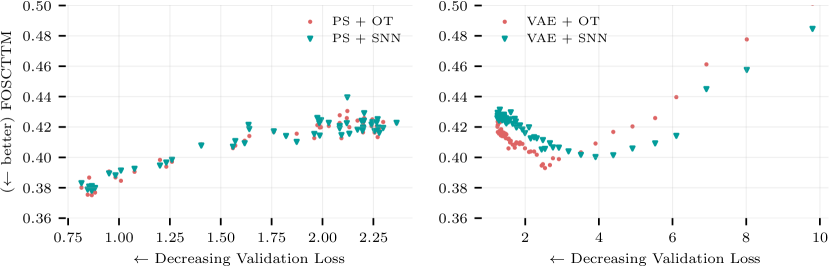
When the assumptions are satisfied, the success of our propensity score method hinges on how well we can learn the conditional distributions . Thus, the validation cross entropy can be used as a tractable metric that can serve as a model selection monitor for the matching performance, which would be unknown in practice. The effectiveness of such a monitor is validated in our experiments, even on real-world CITE-seq data, where we see that a lower validation loss typically corresponds to higher matching performance which is not the case for the VAE (Figure 3). We suspect that this is precisely due to the additional requirement that the VAE minimize a reconstruction loss, in addition to the classification cross-entropy.
6.2 Results
We checkpoint the classifier and VAEs at the lowest validation loss and report their metrics on a held out test set over 10 random seeds. Note that this does not necessarily select the embedding model that exhibits optimal matching, but instead the best model to select without validating against ground truth matching metrics, see Figure 3. We further used 10 random seeds for training the MLP used for modality prediction. scGLUE is trained according to the public implementation, which uses learning rate reduction and early stopping strategies. SCOT is a non-iterative approach and thus we directly report its results.
We found that OT matching on propensity scores consistently outperforms other methods on all metrics, typically followed by SNN matching on propensity scores, or OT matching on VAE embeddings. Furthermore, both the VAE and propensity score, which leverage experimental label information, tend to perform better. This suggests that using the propensity score as embeddings for matching, and using OT to perform the final matching both independently improve matching performance. Curiously, SCOT performs well on the MSE metric for image data, but only places slightly above random in the trace metric. This indicates that it matches scenes with similar latent coordinates, without placing any significant weight on the exact ground truth. This suggests that exact matches may not be necessary for a method to be useful for downstream tasks.
Surprisingly, using the propensity score embeddings with OT matching appears to improve generalization in the modality prediction task (Table 3), when using the unbiased MSE over a model trained on ground truth pairings (indeed, we observed that the ground truth model had a lower training loss, but higher test loss). This reveals an unexpected benefit of (soft) matching: we can sample from the conditional to minimize the loss Equation 11, which, with a suitable , results in improved generalization compared to the naive MSE. This hinges strongly on the quality of —the resulting from the VAE embeddings results in worse generalization, and in practice the quality of the matching, at least in absolute terms, remains hidden.
7 Conclusion
This work presents a simple algorithm for aligning unpaired data from different modalities. The method is both very general—only requiring a classifier to be trained on each modality—and highly effective for matching, which we show both theoretically and empirically. As a downstream task, we demonstrate the effectiveness of the resulting matchings for cross modality prediction, which leads to better generalization than the ground truth matching on the dataset we evaluated. We suspect that this improved generalization is the result of implicitly enforcing invariance to modality specific information, but more work is needed to evaluate the conditions under which this improved generalization occurs.
References
- Ahuja et al. (2023) Ahuja, K., Mahajan, D., Wang, Y., and Bengio, Y. Interventional causal representation learning. In ICML, 2023.
- Almahairi et al. (2018) Almahairi, A., Rajeshwar, S., Sordoni, A., Bachman, P., and Courville, A. Augmented cyclegan: Learning many-to-many mappings from unpaired data. In ICML, 2018.
- Amodio & Krishnaswamy (2018) Amodio, M. and Krishnaswamy, S. Magan: Aligning biological manifolds. In ICML, 2018.
- Buchholz et al. (2023) Buchholz, S., Rajendran, G., Rosenfeld, E., Aragam, B., Schölkopf, B., and Ravikumar, P. Learning linear causal representations from interventions under general nonlinear mixing. In NeurIPS, 2023.
- Butler et al. (2018) Butler, A., Hoffman, P., Smibert, P., Papalexi, E., and Satija, R. Integrating single-cell transcriptomic data across different conditions, technologies, and species. Nature Biotechnology, 36(5):411–420, 2018.
- Cao et al. (2022) Cao, K., Gong, Q., Hong, Y., and Wan, L. A unified computational framework for single-cell data integration with optimal transport. Nature Communications, 13(1):7419, 2022.
- Cao & Gao (2022) Cao, Z.-J. and Gao, G. Multi-omics single-cell data integration and regulatory inference with graph-linked embedding. Nature Biotechnology, 40(10):1458–1466, 2022.
- Demetci et al. (2022) Demetci, P., Santorella, R., Sandstede, B., Noble, W. S., and Singh, R. Scot: single-cell multi-omics alignment with optimal transport. Journal of Computational Biology, 29(1):3–18, 2022.
- Flamary et al. (2021) Flamary, R., Courty, N., Gramfort, A., Alaya, M. Z., Boisbunon, A., Chambon, S., Chapel, L., Corenflos, A., Fatras, K., Fournier, N., Gautheron, L., Gayraud, N. T., Janati, H., Rakotomamonjy, A., Redko, I., Rolet, A., Schutz, A., Seguy, V., Sutherland, D. J., Tavenard, R., Tong, A., and Vayer, T. Pot: Python optimal transport. Journal of Machine Learning Research, 22(78):1–8, 2021.
- Foster et al. (2022) Foster, A., Vezér, Á., Glastonbury, C. A., Creed, P., Abujudeh, S., and Sim, A. Contrastive mixture of posteriors for counterfactual inference, data integration and fairness. In ICML, 2022.
- Genevay et al. (2018) Genevay, A., Peyré, G., and Cuturi, M. Learning generative models with sinkhorn divergences. In AISTATS, 2018.
- Gossi et al. (2023) Gossi, F., Pati, P., Chouvardas, P., Martinelli, A. L., Kruithof-de Julio, M., and Rapsomaniki, M. A. Matching single cells across modalities with contrastive learning and optimal transport. Briefings in Bioinformatics, 24(3), 2023.
- Gresele et al. (2020) Gresele, L., Rubenstein, P. K., Mehrjou, A., Locatello, F., and Schölkopf, B. The incomplete rosetta stone problem: Identifiability results for multi-view nonlinear ica. In UAI, 2020.
- Gutmann & Hyvärinen (2010) Gutmann, M. and Hyvärinen, A. Noise-contrastive estimation: A new estimation principle for unnormalized statistical models. In AISTATS, 2010.
- Hartford et al. (2017) Hartford, J., Lewis, G., Leyton-Brown, K., and Taddy, M. Deep iv: A flexible approach for counterfactual prediction. In ICML, 2017.
- Khemakhem et al. (2020) Khemakhem, I., Kingma, D. P., Monti, R. P., and Hyvärinen, A. Variational autoencoders and nonlinear ICA: A unifying framework. In AISTATS, 2020.
- Korsunsky et al. (2019) Korsunsky, I., Millard, N., Fan, J., Slowikowski, K., Zhang, F., Wei, K., Baglaenko, Y., Brenner, M., Loh, P.-r., and Raychaudhuri, S. Fast, sensitive and accurate integration of single-cell data with harmony. Nature Methods, 16(12):1289–1296, 2019.
- Lance et al. (2022) Lance, C., Luecken, M. D., Burkhardt, D. B., Cannoodt, R., Rautenstrauch, P., Laddach, A., Ubingazhibov, A., Cao, Z.-J., Deng, K., Khan, S., et al. Multimodal single cell data integration challenge: Results and lessons learned. In NeurIPS 2021 Competitions and Demonstrations Track, pp. 162–176, 2022.
- Liu et al. (2019) Liu, J., Huang, Y., Singh, R., Vert, J.-P., and Noble, W. S. Jointly Embedding Multiple Single-Cell Omics Measurements. In 19th International Workshop on Algorithms in Bioinformatics (WABI 2019), 2019.
- Liu et al. (2017) Liu, M.-Y., Breuel, T., and Kautz, J. Unsupervised image-to-image translation networks. NeurIPS, 2017.
- Radford et al. (2021) Radford, A., Kim, J. W., Hallacy, C., Ramesh, A., Goh, G., Agarwal, S., Sastry, G., Askell, A., Mishkin, P., Clark, J., et al. Learning transferable visual models from natural language supervision. In ICML, 2021.
- Rubin (1974) Rubin, D. B. Estimating causal effects of treatments in randomized and nonrandomized studies. Journal of Educational Psychology, 66(5):688, 1974.
- Schiebinger et al. (2019) Schiebinger, G., Shu, J., Tabaka, M., Cleary, B., Subramanian, V., Solomon, A., Gould, J., Liu, S., Lin, S., Berube, P., et al. Optimal-transport analysis of single-cell gene expression identifies developmental trajectories in reprogramming. Cell, 176(4):928–943, 2019.
- Spivak (2018) Spivak, M. Calculus on Manifolds: a Modern Approach to Classical Theorems of Advanced Calculus. CRC press, 2018.
- Squires et al. (2023) Squires, C., Seigal, A., Bhate, S. S., and Uhler, C. Linear causal disentanglement via interventions. In ICML, 2023.
- Sturma et al. (2023) Sturma, N., Squires, C., Drton, M., and Uhler, C. Unpaired multi-domain causal representation learning. In NeurIPS, 2023.
- Tong et al. (2020) Tong, A., Huang, J., Wolf, G., Van Dijk, D., and Krishnaswamy, S. Trajectorynet: A dynamic optimal transport network for modeling cellular dynamics. In ICML, 2020.
- van den Oord et al. (2018) van den Oord, A., Li, Y., and Vinyals, O. Representation learning with contrastive predictive coding. arXiv preprint arXiv:1807.03748, 2018.
- Villani (2009) Villani, C. Optimal Transport: Old and New, volume 338. Springer, 2009.
- von Kügelgen et al. (2023) von Kügelgen, J., Besserve, M., Wendong, L., Gresele, L., Kekić, A., Bareinboim, E., Blei, D. M., and Schölkopf, B. Nonparametric identifiability of causal representations from unknown interventions. In NeurIPS, 2023.
- Xi & Bloem-Reddy (2023) Xi, Q. and Bloem-Reddy, B. Indeterminacy in generative models: Characterization and strong identifiability. In AISTATS, 2023.
- Yang et al. (2021) Yang, K. D., Belyaeva, A., Venkatachalapathy, S., Damodaran, K., Katcoff, A., Radhakrishnan, A., Shivashankar, G., and Uhler, C. Multi-domain translation between single-cell imaging and sequencing data using autoencoders. Nature Communications, 12(1):31, 2021.
- Zhu et al. (2017) Zhu, J.-Y., Park, T., Isola, P., and Efros, A. A. Unpaired image-to-image translation using cycle-consistent adversarial networks. In Proceedings of the IEEE international conference on computer vision, pp. 2223–2232, 2017.
Appendix A Cyclic monotonicity
We can see the monotonicity requirement Equation 8 as the monotonicity of the function with graph . In higher dimensions, we require that the “graph” satisfies the following cyclic monotonicity property (Villani, 2009):
Definition A.1.
The collection is said to be -cyclically monotone for some cost function , if for any , and any subset of pairs , we have
| (13) |
Importantly, we define , so that the sequence represents a cycle.
Note in our setting, the OT cost function is the Euclidean distance, . It is known that the OT solution must satisfy cyclic monotonicity. Thus, if the true pairing is uniquely cyclically monotone, we can recover it with OT.
Appendix B Shared Nearest Neighbours Matching
Using the propensity score distance, we can compute nearest neighbours both within and between the two modalities. We follow Cao & Gao (2022) and compute the normalized shared nearest neighbours (SNN) between each pair of observations as the entry of the matching matrix. For each pair of observations , we define four sets:
-
•
: the k nearest neighbours of amongst . is considered a neighbour of itself.
-
•
: the k nearest neighbours of amongst .
-
•
: the k nearest neighbours of amongst .
-
•
: the k nearest neighbours of amongst . is considered a neighbour of itself.
Intuitively, if and correspond to the same underlying propensity score, their nearest neighbours amongst observations from each modality should be the same. This is measured as a set difference between and , and likewise for and . Then, a modified Jaccard index is computed as follows. Define
| (14) |
the sum of the number of shared neighbours measured in each modality. Then, we compute the following Jaccard distance to populate the unnormalized matching matrix:
| (15) |
where notice that , since each set contains distinct neighbours, and thus , as with the standard Jaccard index. Then, we normalize each row to produce the final matching matrix:
| (16) |
Note is always well defined because and are always considered neighbours of themselves.
Lemma B.1.
has at least one non-zero entry in each of its rows and columns for any number of neighbours .
Proof.
We prove that for at least one in each , which is equivalent to . Fix an arbitrary . by definition is the same set for every . By the assumption of it is non-empty, so there exists . Since is a neighbour of itself, we have , showing that . The same reasoning applied to 11 and 12 also shows that for at least one in each . ∎
Appendix C Omitted Proofs
C.1 Proof of Proposition 3.1
Proof.
Let denote the observed modality and be the unique corresponding latent values. By injectivity,
| (17) |
for , since we assumed in Section 3. Since this holds pointwise, it shows that as random variables. Now, a classical result of Rubin (1974) gives that , and that for any other function (a balancing score) such that , we have . The first property written in information theoretic terms yields,
| (18) |
since as random variables, as required. ∎
C.2 Proof of Proposition 3.2
Proof.
In what follows, we write to be the restriction to its domain where it is strictly positive. The -th dimension of the propensity score can be written as
| (19) |
which, when restricted to be strictly positive, maps to the relative interior of the -dimensional probability simplex. Consider the following transformation:
| (20) | |||
| (21) |
where is constant in , and that . Ignoring the constant first dimension, we can view as an invertible map to . Under this convention, the map is smooth ( is smooth, and the densities are smooth by assumption). Since it is smooth, it cannot be injective if (Spivak, 2018). Finally, since is bijective, this implies that cannot be injective. ∎
Appendix D Experimental Details
D.1 Evaluation Metrics
We can evaluate how well samples are matched using the ground truth provided by our datasets. In these cases, the dataset sizes are necessarily balanced, so that . In each case, the metric is a function of a matching matrix , which recall we compute within samples with the same . Our reported results are then averaged over each cluster. We randomize the order of the datasets before performing the matching to avoid pathological cases.
Trace Metric Assuming the given indices correspond to the true matching, we can compute the average weight on correct matches, which is the normalized trace of :
| (22) |
As a baseline, notice that a uniformly random matching that assigns for each cell yields and hence will obtain a metric of . This metric however does not capture potential failure modes of matching. For example, exactly matching one sample, while adversarially matching dissimiliar samples for the remainder also yields a trace of , which is equal to that of a random matching.
Latent MSE Because the image dataset is synthetic, we have access to the ground truth latent values that generated the images, . We compute matched latents as , the mean projection according to the matching matrix. Then, to evaluate the quality of the matching, we compute the MSE:
| (23) |
FOSCTTM For the CITE-seq dataset, we can use the Fraction Of Samples Closer Than the True Match (FOSCTTM) (Demetci et al., 2022; Liu et al., 2019) as an alternative matching metric. First, we distribute the mass of to as , resulting in a projection of the first modality in the space of the second modality. Then, we can compute a cross-modality distance as follows. For each point in , we compute the Euclidean distance to each point in , and compute the fraction of samples in that are closer than the true match. We also repeat this for each point in , computing the fraction of samples in in this case. That is, assuming again that the given indices correspond to the true matching, we compute:
| (24) | |||
| (25) |
where notice that this is a function of through the computation . As a baseline, we should expect a random matching, when distances between points are randomly distributed, to have an FOSCTTM of .
D.2 Models
In this section we describe experimental details pertaining to the propensity score and VAE (Yang et al., 2021). SCOT (Demetci et al., 2022) and scGLUE (Cao & Gao, 2022) are used according to tutorials and recommended default settings by the authors.
Loss Functions The propensity score approach minimizes the standard cross-entropy loss for both modalities, as implemented in PyTorch 2.0.1. The VAE includes, in addition to the standard ELBO loss (with parameter on the KL term), two cross-entropy losses based on classifiers from the latent space: one, weighted by a parameter to classify as in the propensity score, and another, weighted by a parameter , that classifies which modality the latent point belongs to.
Hyperparameters and Optimization We use the Adam optimizer with learning rate and one cycle learning rate scheduler. We follow Yang et al. (2021) and set , , but found that (compared to in Yang et al. (2021)) resulted in better performance. We used batch size 256 in both instances and trained for either 100 epochs (image) or 250 epochs (CITE-seq).
Architecture For the synthetic image dataset, we use an 5-layer convolutional network (channels ) with batch normalization and leaky ReLU activations, with linear heads for classification (propensity score and VAE) and posterior mean and variance estimation (VAE). For the VAE, the decoder consists of convolutional transpose layers that reverse those of the encoder. For the CITE-seq dataset, we use a 5-layer MLP with constant hidden dimension , with batch normalization and ReLU activations (adapted from the fully connected VAE in Yang et al. (2021)) as both the encoder and VAE decoder. We use the same architecture for both modalities, RNA-seq (as we process the top 200 PCs) and protein.
Optimal Transport We used POT (Flamary et al., 2021) to solve the entropic OT problem, using the log-sinkhorn solver, with regularization strength .
D.3 Data
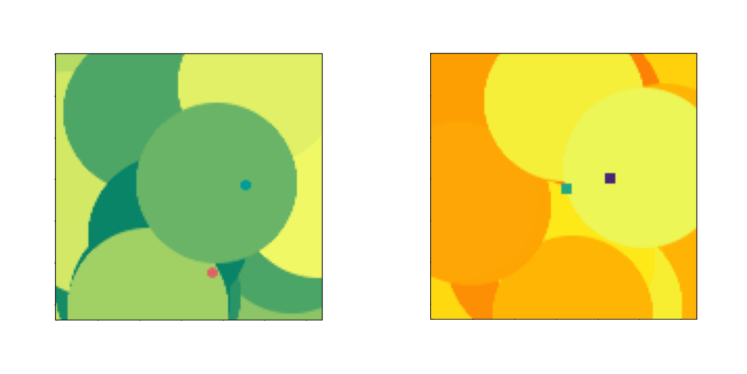
Synthetic Data We follow the data generating process Section 3 to generate coloured scenes of two simple objects (circles, or squares) in various orientations and with various backgrounds. The position of the objects are encoded in the latent variable , which is perturbed by a do-intervention (setting to a fixed value) randomly sampled for each . Each object has an and coordinate, leading to a -dimensional , for which we consider separate interventions each, leading to different settings. The modality then corresponds to whether the objects are circular or square, and a fixed transformation of , while the modality-specific noise controls background distortions. Scenes are generated using a rendering engine from PyGame as . Example images are given in Figure 4.
CITE-seq Data
We also use the CITE-seq dataset from Lance et al. (2022) as a real-world benchmark (obtained from GEO accession GSE194122). These consist of paired RNA-seq and surface level protein measurements, and their cell type annotations over different cell types. We used scanpy, a standard bioinformatics package, to perform PCA dimension reduction on RNA-seq by taking the first 200 principal components. The protein measurements (134-dimensional) was processed in raw form. For more details, see Lance et al. (2022).