FLEXIS: FLEXible Frequent Subgraph Mining using Maximal Independent Sets
Abstract.
Frequent Subgraph Mining (FSM) is the process of identifying common subgraph patterns that surpass a predefined frequency threshold. While FSM is widely applicable in fields like bioinformatics, chemical analysis, and social network anomaly detection, its execution remains time-consuming and complex. This complexity stems from the need to recognize high-frequency subgraphs and ascertain if they exceed the set threshold. Current approaches to identifying these patterns often rely on edge or vertex extension methods. However, these strategies can introduce redundancies and cause increased latency. To address these challenges, this paper introduces a novel approach for identifying potential -vertex patterns by combining two frequently observed -vertex patterns. This method optimizes the breadth-first search, which allows for quicker search termination based on vertices count and support value. Another challenge in FSM is the validation of the presumed pattern against a specific threshold. Existing metrics, such as Maximum Independent Set (MIS) and Minimum Node Image (MNI), either demand significant computational time or risk overestimating pattern counts. Our innovative approach aligns with the MIS and identifies independent subgraphs. Through the “Maximal Independent Set” metric, this paper offers an efficient solution that minimizes latency and provides users with control over pattern overlap. Through extensive experimentation, our proposed method achieves an average of 10.58x speedup when compared to GraMi and an average 3x speedup when compared to T-FSM.
1. Introduction
Frequent Subgraph Mining (FSM) has seen significant interest recently due to its applications in various domains such as chemical analysis (Kong et al., 2022), bioinformatics (Mrzic et al., 2018), social network anomaly detection (Bindu and Thilagam, 2016), and Android malware detection (Martinelli et al., 2013). FSM involves identifying recurring subgraphs in a larger graph that exceed a predefined frequency threshold. Despite its growing importance, FSM poses challenges due to its time-consuming and complex nature, especially as it requires identifying high-frequency subgraphs and verifying if they surpass a set threshold - an NP-complete problem. FSM is generally solved in two steps, namely, (1) Generation Step: identifying potential high-frequency subgraphs within the large graph, and (2) Metric Step: determining if these subgraphs occur more than a predefined threshold. Thus, to effectively solve the problem, determining an efficient method for both steps is important.
Considerable research efforts have been directed towards both steps of this approach. Generation Step has been tackled using techniques based on edge extension or vertex extension. In the case of edge extension methods, there are two main approaches. (1) A possible edge subgraph is derived from two frequent -subgraphs. The process of merging two viable subgraphs sharing identical edge subgraphs is detailed in multiple works (Kuramochi and Karypis, 2004, 2005). However, these approaches are either used for transactional graphs, in which the occurrence of patterns in multiple graphs is considered, as opposed to our single graph approach, or the extension is on an edge level. The main disadvantage of this approach is that during the breadth-first search, the candidate pattern graphs with the same number of vertices are placed at different levels hence curbing the early termination criteria based on the number of vertices and support value. (2) The other approach involves the addition of an edge to all frequent -subgraphs followed by eliminating redundancies (Yuan et al., 2023; Elseidy et al., 2014). This approach generates a lot of redundancies and removing them takes a considerable amount of time.
In the case of the vertex extension methods as illustrated by works such as (Chen et al., 2020, 2022; Yao et al., 2020; Chen et al., 2021), the potential -vertex subgraphs are established by exhaustively generating all feasible extensions of -vertex frequent subgraphs, and eliminating redundancies. This method is similar to the second edge extension method and thus suffers from the same drawbacks.
This paper proposes to identify potentially frequent subgraph patterns directly in the pattern space. Our approach generates -vertex candidate patterns by merging two -vertex patterns that have been already identified as frequent. The implementation of this merging strategy tackles several non-trivial challenges, including the identification of suitable merge points that maintain the graph’s meaningful connectivity, handling labels and attributes on vertices and edges to ensure coherent merged patterns, and ensuring that the merged patterns are unique and non-redundant by checking for automorphisms and determining canonical forms.
The Metric Step in Frequent Subgraph Mining has seen advancements, particularly with the Maximum Independent Set (MIS) metric. This metric is known for its accuracy and calculates pattern frequency by counting disjoint, independent patterns in the data graph. However, its NP-complete nature requires considerable computational time. An alternative, the Mininum Image (MNI), finds the maximum count of independent sets for a pattern but can result in non-disjoint sets and potential vertex overlap, leading to pattern count overestimation. (Yuan et al., 2023) introduced a fractional-score method based on MNI, reducing overestimation by factoring in each vertex’s contribution to a pattern. Despite fewer false positives, this method still faces significant inaccuracies (Yuan et al., 2023). A limitation of both MIS and MNI is the lack of user control over the overlap between identified patterns.
In contrast, our proposed approach introduces a mechanism to align with the MIS, which exclusively identifies independent patterns without vertex overlap. This is achieved through the utilization of Maximal Independent Set (mIS). mIS is an approximation of MIS. We leverage a mathematical relationship that exists between these metrics, which enables us to establish the lower bound of support for the mIS metric, based on the support for the MIS metric. The upper bound corresponds to the support value for MIS. Users can define the degree of overlap with the MIS metric by selecting the interpolation level, referred to as the slider value. This way, they have control over the extent of overlap with the MIS metric, offering a metric applicable across various applications. For instance, in network analysis, a degree of overestimation may be acceptable, whereas, in fields like chemical composition analysis or biomedical research, precision is of paramount importance, even if it means potentially missing some patterns. While the overlap chosen by the user may lead to missing some patterns, it ensures that the patterns identified are accurate.
This paper makes the following contributions,
-
•
It proposes an innovative method for generating candidate subgraph patterns by merging two frequently occurring smaller subgraph patterns, each with vertices, to efficiently form potential larger subgraph patterns with vertices to effectively prune the search space.
-
•
The paper introduces a new metric based on the Maximal Independent Set, allowing for the enumeration of pattern graphs within a data graph, with a user-defined slider for controlling the overlap with MIS metric, enhancing both accuracy and flexibility in frequent subgraph mining.
-
•
It conducts extensive experiments to demonstrate the efficiency of the proposed algorithms, showing a significant improvement in computational time and memory usage compared to existing graph mining methods like GraMi and T-FSM.
2. Preliminaries
In this section, we introduce the definitions and terminologies for the terms used in the rest of the paper.
2.1. General Graph Terminologies
2.1.1. Articulation Vertex
An articulation vertex (AV) in an undirected graph is a vertex whose removal disconnects the graph. An AV in a directed graph is defined by making all directed edges undirected and then using the definition for undirected graphs.
2.1.2. Graph Isomorphism
Two labeled graphs and , where each vertex has label , are isomorphic if there exists a bijection such that for any two vertices , and for each .
2.1.3. Automorphism
An automorphism of a graph is a special case of graph isomorphism, where a graph is mapped onto itself. Formally, an automorphism of a labeled graph is a bijection such that for any two vertices , and for each . An automorphism is thus a permutation of . The set of all automorphisms of a graph can be produced using generators. Generators are a compact subset of automorphisms whose composition results in the generation of its automorphisms.
Graph (Figure 1(a)) has two automorphisms: (1) the identity permutation (1,2,3) which maps each vertex onto itself and
(2) permutation (3,2,1) which maps and to each other and onto itself - note this holds because and have the same color (label). In this instance, the set of generators is the same as the set of automorphisms. If all vertices in had the same label, it would have six automorphisms corresponding to the 3! permutations of its vertices. These can be generated by using two generators: (2,1,3) which swaps and and (1,3,2) which swaps and .
2.1.4. Subgraph Isomorphism
Given vertex-labeled data and pattern graphs and , respectively, and a set of labels , where each vertex has a label : is subgraph isomorphic to (is a subgraph of) if there exists an injective function such that (1) for all and (2) for all . Note: our definition of subgraph isomorphism does not require an edge in if one exists between the corresponding vertices in .
2.1.5. Bliss
The Bliss library (Junttila and Kaski, 2007a, 2011) is used to determine whether two vertex-labeled graphs (undirected or directed) and are isomorphic. It computes (1) a hash (which may not be unique) and (2) a canonical form (which is unique) for both and . If the hashes are unequal, and are quickly determined to be non-isomorphic. If the hashes are equal, their canonical forms are checked and if equal, and are isomorphic. Bliss also computes generators and automorphisms of a graph.
2.2. Graph Mining
Frequent subgraph mining (FSM) identifies pattern graphs that are subgraphs of a given data graph that occur a certain number of times. This paper focuses on FSM (Bringmann and Nijssen, 2008) on labeled, directed graphs. However, our techniques can be trivially extended to unlabeled and/or undirected graphs. Figure 1 illustrates these concepts. Both patterns (Figure 1(a)) and (Figure 1(b)) are subgraphs of data graph (Figure 1(c)). Specifically, can be seen to be a subgraph of using six functions that map to: (i) , (ii) , (iii) , (iv) , (v) , (vi) .
Recall that we approach the graph mining problem in two steps: generation (derive candidate subgraphs) and metric (determine which candidate subgraphs occur in the data graph and are frequent). Using this terminology, both and may be viewed as candidate subgraphs. Although we have not yet formally defined how we count occurrences (i.e., the metric), a threshold of 7 would result in being classified as infrequent in .
2.2.1. Anti-monotone Property
Let and be subgraphs of data graph such that is a subgraph of and is a k-size pattern while is -size pattern. Anti-monotone property states the number of instances of number of instances of in .
2.3. Generation Step terminologies
2.3.1. Core Graph and Marked Vertex
A core graph is obtained from a pattern graph by disconnecting one of its vertices along with its incident edges. denotes the core graph obtained by disconnecting vertex from pattern graph . The disconnected vertex is referred to as the marked vertex of the core graph. denotes the core graph (Figure 2(a)) formed by disconnecting vertex from pattern ; is the marked vertex of .
2.3.2. Core Graph Isomorphism
Two core graphs are isomorphic iff the core graphs with marked vertices excluded are isomorphic. For example, is isomorphic to .
2.3.3. Core Groups
The set of all core graphs generated from patterns of the same size, grouped by isomorphic core graphs, is collectively referred to as core groups. A single core group is represented as a ¡key, value¿ pair, where the key is a core graph without the marked vertex and the value is a list of all core graphs that are isomorphic to the key and to each other. Three core groups are generated from pattern graphs and (Figure 1(a) and Figure 1(b)): , , .
2.3.4. Extended Core Graphs
Although the preceding definitions assume that only vertices are labeled, there exist applications where edges are also labeled. We are able to transform edge-labeled graphs into vertex-labeled graphs as follows: an edge with label is replaced with two edges and . The newly introduced vertex is assigned label . Figure 2(c) shows the extended CoreGraph of Figure 2(a), in which is introduced in edge and is introduced in edge .
2.4. Metric Step
The metric step counts the number of occurrences of each candidate pattern in the data graph and determines whether it is frequent. We next review metrics such as MIS, MNI and FS that have been used in the literature to determine subgraph frequency counts and introduce our metric, the mIS, a key contribution of this paper. The MIS is the gold standard in pattern frequency counting due to its accuracy in providing exact counts. However, its high computational complexity has made it challenging to use. The MNI serves as a faster, approximate alternative to MIS but can significantly overestimate pattern counts. The Fractional-Score (FS) metric is a variation of MNI that attempts to address the overestimation but still occasionally overestimates certain patterns. To address these drawbacks, we propose mIS, a metric that preserves the independent set property of MIS while providing the flexibility to choose between overestimation or underestimation of patterns. Additionally, mIS has the advantage of running with similar runtimes as MNI, making it a practical choice for subgraph mining tasks.
Let be the set of all possible mappings from . Each mapping represents an injective function represented by a list of of pairs of the form which maps each to vertex .
2.4.1. Independent Set
An independent set , is a subset of where for any two distinct mappings , in , and for any vertex pair and any vertex pair , it holds that . That is there are no two mappings that share the same vertex in . For instance, in the case of pattern , an independent set could be any one of the mappings in Figure 3 except Figure 3(e).
2.4.2. Maximum Independent Set (MIS) (Kuramochi and Karypis, 2005)
MIS is an independent set of maximum size among all independent sets; i.e., there is no other independent set with a greater number of mappings. For pattern , Figure 3(d) is the MIS.
2.4.3. Maximal Independent Set (mIS)
mIS is an independent set such that there is no possible addition of a mapping that preserves independence. For pattern , maximal independent sets are depicted in Figures 3(c) and 3(d). However, Figures 3(a) and 3(b) are not mIS, since additional mappings can be added that preserve independence.
2.4.4. Mininum Image (MNI) (Elseidy et al., 2014)
Recall that is the set of all possible mappings from . Let be the injective mapping used in mapping . For each vertex , define as the set of unique images of in under these mappings. MNI of in is . For in , , , giving an MNI of 3 (Figure 3(e)).
2.4.5. Fractional-Score (Yuan et al., 2023)
A Fractional-Score based method is an extension of MNI, which uses fractional scores to reduce overestimation. The fractional score is determined based on the contribution of each vertex to its neighbors. For instance, in Figure 1, for data graph and pattern graph, the contribution of to is , this is because there are two vertices with the same label that can equally contribute to. With this value, the total contribution of each vertex to a specific label is calculated to be . However, this value is still more than the MIS value of 2. Thus, the fractional score method still overestimates the support value.
3. FLEXIS
The FLExible Frequent Subgraph Mining using MaXimal Independent Set (FLEXIS) framework presents an approach for discovering frequent subgraphs within a data graph.
3.1. Methodological Contributions
3.1.1. Contribution 1
The previous section introduced a new metric mIS which adopts the best features of MIS and MNI. It crucially retains the independence property (i.e., that vertices do not overlap) of MIS and thus overcomes the overestimation problem of MNI (Yuan et al., 2023). Like MNI, mIS can be computed quickly, whereas computing MIS is expensive due to its NP-hardness. In addition, mIS provides a user-controlled parameter that can be used to tune the accuracy-speed trade-off of the algorithm. The theoretical basis for this is the important approximation result included below.
Theorem 3.1.
Given a pattern graph with vertices. Let denote the number of mappings in a maximal (mIS) independent set and the number of mappings in a maximum independent set. Then .
Proof.
follows immediately from the definitions of mIS and MIS. If the second inequality is false, we have . The mappings of the mIS together comprise distinct vertices in the data graph due to the independence property of mIS. Each of these vertices from the mIS can be allocated to a different mapping of MIS. However, since , it follows that there is at least one mapping in MIS whose data graph vertices do not include any of the mIS vertices. Then, can be added to the mIS, contradicting that it was maximal. ∎
We show that the bound in Theorem 3.1 is tight using the example in Figure 4 with pattern containing vertices. An MIS computation yields mappings shown in blue, green, yellow, and orange. A mIS computation either picks the same 4 mappings as MIS or picks the single mapping (i.e., ) shown in red. The latter scenario gives , yielding a tight bound.
red: , blue: , green: , yellow: , orange:
In classical FSM, patterns that occur at least (the support) times in the data graph are considered frequent. We instead consider a pattern to be frequent if it occurs at least times.
| (1) |
where denotes the number of vertices in the pattern and the user-defined parameter is in the range . Notice that when , and when , . The choice of as one of the endpoints results from the second inequality of Theorem 3.1, which shows that mIS approximates MIS to within a factor of . Relative to the “gold standard” MIS metric, guarantees that there will be no false positives while guarantees there will be no false negatives. A in between trades off between these two scenarios. We discuss these with some examples below.
The number of occurrences of in (Figure 1) depends on the metric: e.g., MIS gives 2 (Figure 3(d)), while MNI gives 3 (Figure 3(e)). If run to completion, mIS gives either 1 (Figure 3(c)) or 2 (Figure 3(d)). Our implementation of mIS allows us to terminate when a given is reached. Thus, if , mIS could return the match shown in Figure 3(a) or Figure 3(b) in addition to Figure 3(c). Now, assume so that . If , is not considered frequent under MIS and mIS, but is frequent under MNI (which allows overlapping vertices). This example illustrates the additional pruning that occurs when using mIS relative to MNI. If as before, but giving , FLEXIS gives either Figure 3(c) and declares infrequent or Figure 3(d) and correctly declares frequent. However, if and , for a size-3 pattern. Now, FLEXIS terminates after finding Figure 3(a), Figure 3(b), or Figure 3(c). Here, FLEXIS correctly determines that is frequent.
When , FLEXIS overestimates the number of frequent patterns. This approximates the behavior of MNI, which also overestimates the number of frequent patterns, but never reports an infrequent pattern. However, early termination allows FLEXIS to run faster than MIS.
This versatility grants users the flexibility to fine-tune the trade-off between accuracy and processing time, tailoring the metric to suit the specific needs of their applications. It is important to emphasize that our approach achieves performance levels akin to both MNI and MIS but at significantly reduced computational time, maintaining nearly equivalent accuracy when compared to traditional methods.
3.1.2. Contribution 2
The concept of merging two -size frequent patterns to find possible -size frequent patterns has been utilized previously (Kuramochi and Karypis, 2005). In that work, the size of the pattern graph was defined as the number of edges, whereas we define size as the number of vertices. (A graph with 3 vertices and 2 edges thus has size 2 in their method and size 3 in ours.) This distinction is important because the vertex-based approach prunes the search space more effectively, resulting in better performance.
FLEXIS starts by identifying all size-2 patterns (edges) in the data graph. It then uses a matcher (vf3matcher) to determine which size-2 patterns are frequent. These are merged to create candidate patterns of size 3. The candidate patterns are evaluated to identify the frequent ones, which are then merged, etc. We illustrate this using size-3 patterns and (from Figure 1) and merging them to form size-4 candidate pattern graphs (Figure 5).
To gain intuition about why this approach prunes more efficiently relative to edge-based merging, consider a data graph with vertices and . No frequent pattern can have more than vertices because mIS does not permit overlap. Patterns of size 5 or more do not need to be considered and can be pruned. FLEXIS will not require more than three merging steps to generate candidates (, , ). Edge-based merging (Kuramochi and Karypis, 2005) requires more merging steps and incurs more runtime.
3.1.3. Summary
Our method has the following advantages, (1) mISis closely related to the actual frequent pattern count metric MIS, while providing comparable or better speedup than MNI. (2) mISis the first metric that allows the user to control the accuracy-speed trade-off. (3) FLEXISis the first method that uses the merging of two frequent patterns based on vertices rather than edges, resulting in a faster search process
3.2. Algorithmic flow of FLEXIS
FLEXIS outlined in Algorithm 1 consists of the following steps:
-
(1)
Candidate Pattern Generation (Generation Step): Initially, FLEXIS generates all size-2 candidate patterns (i.e., edges) () from the data graph (4).
-
(2)
Finding Frequent Patterns (Metric Step): All frequent patterns () within the candidate set are found by utilizing a modified version of Vf3Light (Carletti et al., 2018, 2019), with our custom metric mIS integrated, to ensure non-overlapping vertices (8). Note that the original implementation of Vf3Light uses the MNI metric.
-
(3)
Candidate Pattern Expansion (Next Generation Step): Subsequently, FLEXIS merges frequent patterns () to generate candidate patterns () that are one vertex larger (10).
-
(4)
Steps and continue until all frequent patterns are exhausted (6).
We explain in detail our approach in the Generation and the Metric Steps, in the following sections.
3.2.1. Generation Step
generateNewPatterns (Algorithm 2) combines -vertex frequent patterns to form -vertex candidate patterns. 4 of the function first computes core groups (Section 2.3) from the input set consisting of all -vertex frequent patterns. Each core group identified by is processed in 6 and each pair of core graphs and in the core group is considered in 7. The next step is to merge pairs of core graphs and (10): recall that all core graphs (excluding their marked vertices) in a core group are isomorphic; each core graph can be denoted by a common -vertex component and a disconnected marked vertex. Core graphs differ from each other in that their marked vertices may have different labels and may be attached to the vertices in in different ways. The merge step adds the marked vertices from and to to get a -vertex pattern. However, to generate all possible -vertex candidate patterns, we must explicitly consider every automorphism of (8 and 9). This process generates all non-clique candidate patterns. A modification to this process (merging in a third graph) generates all clique candidate patterns (12) and adds them to the set of candidate patterns. After generating all the , we use RemoveDuplicates to remove duplicate patterns in the candidate generation using Bliss’s canonical form (13).
Figure 5 depicts generateNewPatterns, the process of taking 3-vertex patterns, decomposing them into core graphs, and then merging them to form 4-vertex patterns. Non-clique patterns (such as the top two 4-vertex patterns in Figure 5) are formed by merging two core graphs, whereas clique patterns (such as the bottom 4-vertex pattern in Figure 5) are obtained by additionally merging in a third core graph. The merge operation (Line 8) is a key step within generateNewPatterns. We illustrate it below with examples:
Example 1 (simple merging)
Figure 6 shows three examples that use core graphs derived from patterns and (Figures 1(a) and 1(b)). In Figure 6(a), core graph is merged with itself. Here, two copies of the marked vertex are reattached to the core consisting of vertices and . Figure 6(b) similarly shows being merged with itself. Two copies of are reattached to the core ( and ). Finally, Figure 6(c) shows the result of merging and .
Example 2 (merging with automorphisms)
Next, we illustrate the more complicated scenario of merging with automorphisms in Figure 7. Figure 7(a) shows the 4-vertex pattern . We will merge core graph (obtained from by disconnecting from ) with itself. Figure 7(b) shows the simple merge where two copies of are reattached to .
However, , the triangle obtained by deleting from has an automorphism that maps and to each other (because both have red labels) and to itself. This gives a second merged graph (Figure 7(b)) obtained by reattaching to and attaching a copy of to as a result of the automorphism (we call this Case 1). If had instead originally been connected to (the sole blue vertex in ), the automorphism would not be used since it maps to itself (we call this Case 2). findAutomorphism (called in Line 6 of generateNewPatterns and shown in Algorithm 3) handles these intricacies. A key point is that findAutomorphism does not merely return automorphisms of . Instead, it additionally examines the nature of the connection of the marked vertex to using differentTopology to determine whether we are in Case 1 or Case 2.
We next provide the lemmas and theorem used in the Generation Step.
Lemma 3.2.
Lemma 3.3.
Let be a connected non-clique graph with at least three vertices. has at least two nAV that are not joined by an edge.
Proof.
Since is not a clique, . Consider two vertices and in such that . From Lemma 3.2, and are nAVs. Since , they are not joined by an edge. Thus satisfy the lemma. ∎
Lemma 3.4.
Every connected, non-clique -vertex pattern graph can be generated by merging two connected -vertex pattern graphs (i.e., by the Merge function).
Proof.
Consider any non-clique k-vertex candidate pattern graph . From Lemma 3.3, has two non-articulation vertices and . The two -vertex graphs and , formed respectively by separately removing and from are connected. The process of forming core groups from -vertex patterns in generateNewPatterns(4) removes from and from , giving the common core graph (i.e., with both and removed). The Merge function, essentially the reverse of this process, constructs by starting with the common core graph and adding and with the appropriate edges. ∎
Clique generation: We next extend the idea of merging -vertex pattern graphs to form -vertex cliques. As before, we begin by merging two -vertex pattern graphs. If both are cliques, there is a possibility that they are both sub-patterns of a -vertex clique. Note that the pattern generated by merging two cliques using Merge is not itself a clique (the two marked vertices are not joined by an edge). Therefore, we need to find and merge a suitable third -vertex pattern graph that will supply the missing edge.
Figure 8 shows an example.
Merging Clique Example
We start by merging patterns and (note that both are 3-cliques). Core graphs (obtained from ) and (obtained from ) are merged to form (). has the potential to form a clique by adding an edge between the two marked vertices. We will now identify a third pattern to merge with to complete the clique. An exhaustive search to find such a pattern can be very expensive. We streamline the search by focusing on another core graph obtained from pattern . The idea is that merging two core graphs along one of the 4-clique’s four edges and then a third graph along a diagonal can potentially complete the missing edge of the clique. All core graphs in the core group with ID and a marked vertex label matching that of (i.e., a yellow vertex) are examined to locate the missing edge. In the example, meets these criteria. Merging with gives the clique. Should this core graph be absent, the pattern does not qualify as a candidate clique.
A final post-processing step confirms that all other sub-cliques of size 3 are frequent. In our example, this would mean checking that pattern is frequent.
That is in general,
-
•
Consider two (k-1) cliques whose core graphs have a common (k-2)-subclique in addition to the one marked vertex each.
-
•
After merging the two core graphs, we get a k-clique minus the edge between the two marked vertices ().
-
•
To generate the clique, we need to find a third (k-1) clique, whose (k-2)-subclique core graph is different from the first two, but comes from the same pattern as one of the first two. Also, the marked vertex of the third core graph must have the same label as the marked vertex of the second core graph.
-
•
If such a CoreGraph is found, we merge it with to generate the clique.
-
•
In the post-processing step, we check if all the (k-1)-size sub-graphs of the generated clique are frequent. If yes, the generated clique is set as a candidate pattern. Otherwise, the generated clique is discarded.
The generation of the clique pattern is an extension of the non-clique pattern generation (Algorithm 2). We present the algorithm for generating Clique, as shown in Algorithm 4. The algorithm first starts by checking if the frequent pattern graphs are cliques, as this must be true for the candidate pattern graph to be a clique (trivially true, checked in 4). Then the algorithm strategically searches through the CoreGroups to determine if the missing Clique, which contains the missing edge of the candidate clique is present (7, 8 and 9). Upon finding the required Clique, the algorithm merges the two cliques to form the candidate clique pattern (10). This pattern is then added to the candidate pattern set (12).
Lemma 3.5.
Every clique -size candidate pattern graph can be generated by using three -size frequent clique patterns.
Proof.
Removing a single edge, , from (a clique of -size) results in a non-clique graph, , with vertices as non-articulation vertices. Then according to Lemma 3.4 every non-clique -size pattern graph can be generated by merging two -size frequent patterns. Thus, can be reconstructed from two -size patterns. Since in , every vertex is interconnected except for and , the two -size patterns used to form this non-clique must themselves be cliques.
To reintroduce and restore the complete clique structure of , we seek a third -size pattern that includes both and . This pattern must share a -size subgraph (an anchor) with , ensuring compatibility for the merging process. By definition, merging requires one of ’s vertices to be the marked vertex, and the other to be part of the anchor. By the same reasoning as above this subgraph will also be a clique.
Thus, three (k-1)-size clique patterns are required to form a k-size clique. ∎
Theorem 3.6.
Every candidate pattern can be generated by FLEXIS.
Proof.
The proof follows by induction on the number of vertices . For (the base case), we began by computing all frequent edges in the data graph. In the inductive step, we use Lemmas 3.4 and 3.5 to argue that all -patterns can be generated by merging two or three -patterns.
At each stage, prior to merging, candidate patterns are discarded if they are not frequent. A pattern can only be frequent if all of its - sub-patterns are frequent. Therefore, discarding infrequent sub-patterns does not eliminate any frequent patterns. ∎
3.2.2. Metric/Matcher Step
We check the frequency of the candidate patterns using mIS metric (Section 3.1.1). A candidate pattern is deemed frequent based on a user defined parameter () and support parameter () (Equation 1). We now explain the modifications to Vf3Light for using this metric.
Algorithmic Implementation of Matcher Step
Vf3Light (Carletti et al., 2018, 2019), is a subgraph matching algorithm that is used to find all the embeddings of a pattern graph in the data graph. Vf3Light is a fast and efficient depth-first search-based algorithm that uses matching order and properties of graph isomorphism for early termination and effective pruning. VF3Light finds embeddings that may have automorphisms and overlapping vertices across embeddings. Both of these properties are not desirable for mIS. Thus, we modify VF3Light Vf3LightM) to find mIS of data vertices given the pattern graph. FLEXIS incorporates the following modifications to VF3Light (this description assumes familiarity with VF3Light):
-
(1)
Pruning: Once the embedding succeeds, none of the vertices from that embedding can be used again (independent set violation). So, we modified the matching engine to stop the search for new embeddings with the same root vertex if a match is found. This is done by setting a flag if a match is found. The flag is reset when the root vertex is unstacked from the recursion stack
-
(2)
Independent Set: To make sure the embeddings do not have overlapping vertices, we use a bitmap to store the used vertices. The bitmap is set when a vertex is used in an embedding. The bitmap is shared across different instances of VFState for the same pattern graph to avoid expensive copies.
3.3. Complexity Discussion
A formal asymptotic analysis of FLEXIS is not meaningful because of the inherent complexity of the FSM problem and its subproblems: graph isomorphism and subgraph isomorphism, which are not known to be in . Concretely, the runtime of the algorithm depends on three factors: (1) the number of iterations #iter of the while loop (line 4, Algorithm 1), (2) the run-time of the candidate generation step (generateNewpatterns), and (3) the runtime of the metric step (VF3Matcher). #iter depends inversely on the threshold (the lower its value, the greater the number of candidate patterns and frequent patterns at each iteration and the greater is #iter). depends on Bliss performance to solve the graph isomorphism () problem multiple times. There is presently no polynomial-time algorithm for , nor a proof of NP-completeness. Indeed, this is an active area of research in theoretical Computer Science. The Bliss runtime is not polynomially bounded and depends on characteristics of the input graph, including size and symmetry. Finally, depends on counting the number of instances of a pattern graph in a data graph. This is related to subgraph matching, which is NP-complete. FLEXIS uses VF3Light, which is a backtracking method whose worst-case complexity is exponential.
4. Results
In this section, we evaluate FLEXIS and compare it with GraMi and T-FSM. For this, we utilize the code provided by the authors for GraMi and T-FSM. The original version of GraMi uses Java 17.0.7 and T-FSM uses C++. We implement our method in C++ compiled by g++11. We ran our experiments on Xeon CPU E5-4610 v2 (2.30GHz) on Ubuntu 22.04. Our system has 192 GB DDR3 memory.
Datasets We use real-world graph datasets with varied numbers of vertices, edges and labels. The datasets included are as follows,
- (1)
-
(2)
The soc-Epinions1 (Richardson et al., 2003) is derived from the online social network Epinions.com, a consumer review website.
-
(3)
The Slashdot (Leskovec et al., 2009) reveals user interconnections on Slashdot’s tech news platform.
- (4)
-
(5)
MiCo (Elseidy et al., 2014) dataset is Microsoft co-authorship information.
Table 1 shows the properties of these data graphs. refers to the maximum degree of the graph, is the number of distinct vertex labels, and is the number of distinct edge labels. Vertex and edge labels are randomly assigned to vertices and edges, respectively.
| datagraph | |||||
| Gnutella | 6301 | 48 | 5 | 20777 | 5 |
| Epinions | 75879 | 1801 | 5 | 508837 | 5 |
| Slashdot | 82168 | 2511 | 5 | 948464 | 5 |
| wiki-Vote | 7115 | 893 | 5 | 103689 | 5 |
| MiCo | 100000 | 21 | 29 | 1080298 | 106 |
Metrics The support threshold , in conjunction with a given data graph, and the user defined parameter , serves as the input for the proposed system. The assessment of our system encompasses the execution time incurred during the mining process, analysis of the frequent pattern obtained, and the quantification of memory utilization. We compare our method to both the modifications of the state-of-art algorithm GraMi, namely the AGrami, where is set to , and the baseline GraMi version. We also compare our algorithm with the newest graph mining system T-FSM. In T-FSM we compare our method with both the MNI version and the fractional score version. Conversely, for our developed algorithm denoted as FLEXIS, we present two distinct variants. The first variant entails an implementation absent of any approximation mechanisms. In contrast, the second variant pursues the generation of maximal frequent patterns, a subset of which intersects optimally with those identified by GraMi and T-FSM. Since the problem can run for a long time in the case of large graphs, we restrict the time that both the algorithms run to 30 minutes, after which the system times out. If an algorithm times out then the corresponding values will be missing in the graphs.
4.1. Experimental Setup
Our method uses an undirected data loader and a directed matching algorithm. Thus, to determine the efficiency of performance, only looking at the undirected version might not be fair. Since GraMi has both undirected and directed versions we choose to consider the directed version of GraMi. Moreover, T-FSM proposes a better undirected version of GraMi with some optimizations. Thus, instead of considering the original undirected GraMi, we use the T-FSM version of GraMi, referred to as T-FSM-MNI. We also compare our algorithm with the T-FSM fractional score model (referred in paper as T-FSM). It is important to note that our observations between GraMi and T-FSM do not follow directly from their paper. This is because we consider directed GraMi, while their paper considered the undirected version. Also, since the paper itself postulated the equivalent performance of their MNI version with that of GraMi and better performance of their fractional-score method when compared to GraMi, we do not reinforce this point again in this paper, rather here we use their important observations.
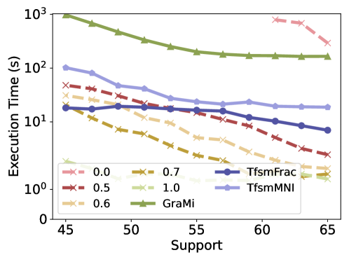


We evaluate the performance of FLEXIS, GraMi, and T-FSM in terms of the time taken to compute frequent subgraphs. The outcomes of both systems were recorded, with a predetermined time limit of minutes. For the sake of clarity for all the other subsequent graphs, we denote GraMi as “GraMi”, T-FSM fractional-based algorithm is shown as “TfsmFrac” while T-FSM MNI is shown as “TfsmMNI”, while numeric identifiers are used for different configurations of FLEXIS, unless mentioned otherwise. Since, FLEXIS is characterized by a parameter range spanning ( slider ()), we use the value chosen for the representation.
4.2. Methodology to select
It is commonly known that the number of times a pattern occurs is overestimated by MNI and as a consequence, the number of patterns classified as frequent is more than the actual value for GraMi. And a similar explanation also holds for T-FSM-MNI. If we take a closer look at the functioning of T-FSM using fractional-score, there is still a considerable overestimation. However, this overestimation is much less than that of GraMi. In contrast, our method spans from over-estimating to under-estimating, with over-estimation happening at a lower value and under-estimation possibly at a higher value. Thus, we postulate that we will merge closer to GraMi at a lower value of , to the T-FSM-MNI at a similar value and to T-FSM, at the same or higher value, depending on the efficiency of fractional-score with those datasets. We follow the following method to determine the most suitable value to compare with GraMi and T-FSM.
-
•
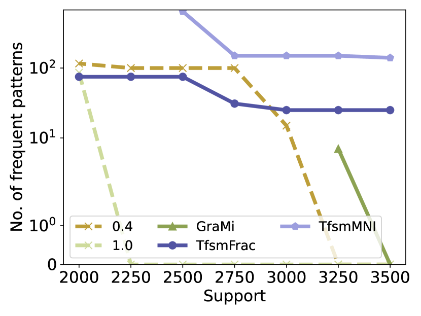
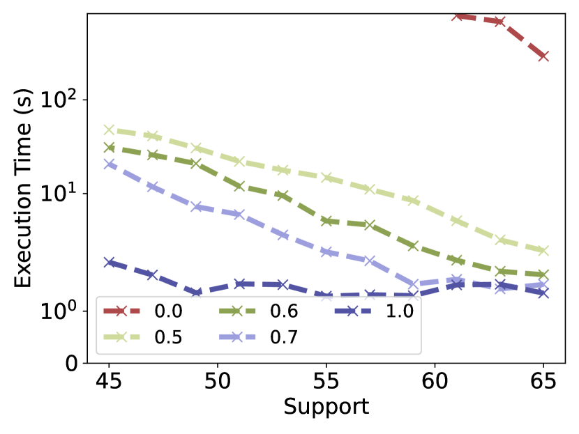
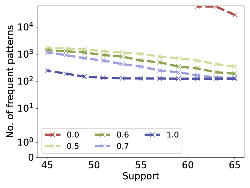
Comparison with different values: We show the time taken (Figure 13(a)) and the number of frequent patterns (Figure 13(b)) for varied values of . As expected, the number of patterns found decreases with an increase in , because of a reduction in overestimation. Also, the time required to find the patterns decreases with an increase in , as the number of patterns searched for decreases. Thus, to be fair in comparison with GraMi and T-FSM, we need to determine the value of in which the number of patterns found matches with that of GraMi and T-FSM.
-
•
Choosing a suitable value: From our experiments, as shown in the Figure 9 most of the values of the execution time of T-FSM (lowest among the other comparing methods) falls closer to our slider value of 0.5. But, as can be seen in the Table 3 the number of frequent patterns in all the three algorithms, namely FLEXIS, GraMi and T-FSM merge at 0.4. To show the similarity in the frequent patterns determined, we used graph isomorphim, and present the results in Table 3. In the table, refers to frequent patterns generated by GraMi, FLEXIS, and T-FSM respectively, and represents the number of vertices. The isomorophism between, GraMi and FLEXIS, T-FSM and FLEXIS are shown as, and respectively. We show only one dataset because of the lack of space. Thus, for the fairness of comparison for the rest of the paper, we will consider the value as .
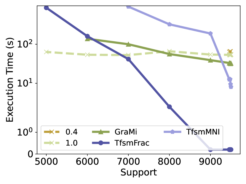
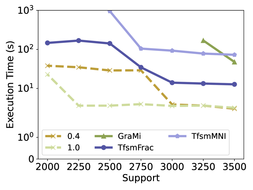
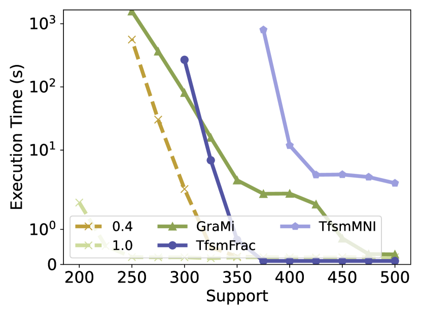
4.3. Execution Time
Execution Time for the Gnutella dataset, across varied slider values, along with GraMi and T-FSM is as shown in Figure 9. For MiCo, Epinions, Slashdot, and wiki-Vote datagraphs in Figure 10. Across Epinions, Slashdot and wiki-Vote, slider performs with an average speed up of 3.02x over T-FSM fractional and 10.58x over GraMi. While with Gnutella, slider with an average speedup of 1.97x over T-FSM fractional and 7.90x over GraMi. Notably, the number of frequent subgraphs exhibits a growth pattern as the support value is decreased.
4.4. Memory Usage
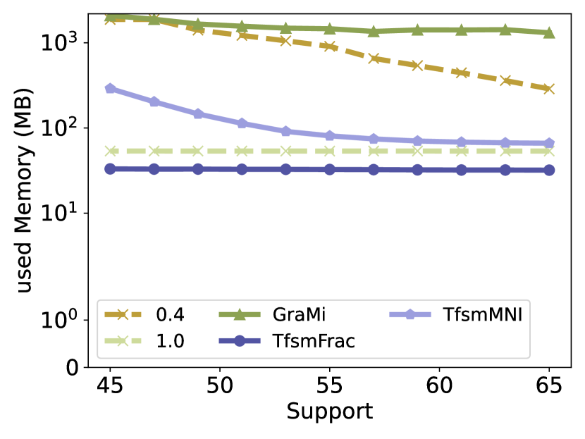
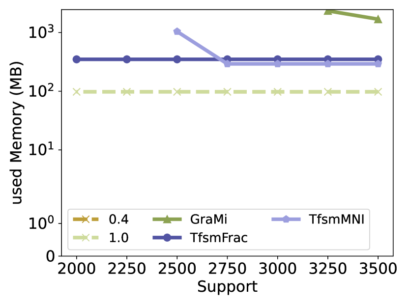
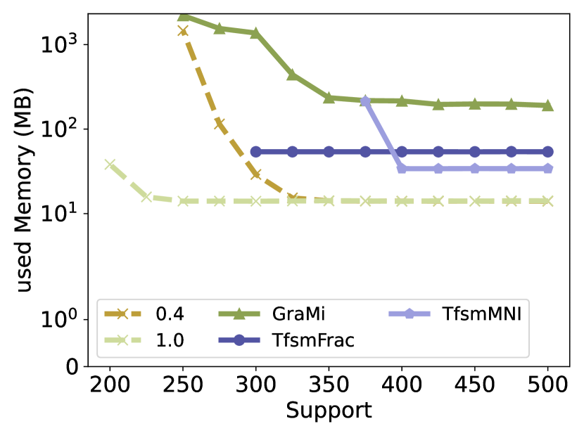
Figure 11 presents memory utilization patterns observed during the processing of the Epinions and wiki-Vote data graphs by FLEXIS, GraMi and T-FSM. It is important to note that instances, where execution was prematurely terminated due to reaching predefined timeout constraints, do not have corresponding memory utilization values represented. As shown in Figure 11, GraMi and T-FSM Fractional uses 8.79x and 1.01x memory than FLEXIS () in average across wiki-Vote, Epinions, and Slashdot. We postulate that the differences in memory utilization patterns emerge between the three systems due to their distinct storage strategies. Specifically, GraMi maintains an expansive repository of both frequent and infrequent graphs, hence higher memory demand. T-FSM is built on top of GraMi and has similar memory requirements, but since T-FSM performs a memory-bound search in the data graph it has lower memory requirements when compared to GraMi. On the contrary, FLEXIS approach stores only the frequent graphs at each level. Since, for the determination of the potential candidates for -size pattern only requires -size pattern, thereby adapting a more resource-efficient memory management framework. It is important to note that with the addition of Gnutella, GraMi and T-FSM Fractional uses 5.83x and 0.64x more memory than FLEXIS. The decrease in memory improvement achieved by FLEXIS can be attributed to more searches required for the Gnutella dataset. This leads to a higher number of frequent and searched patterns.
We can also observe, that as the support value decreases, the memory utilization proportionately increases. This phenomenon occurs due to the greater number of patterns being recognized as frequent as the support threshold decreases. This trend is consistent across both GraMi and our method FLEXIS. In the context of our approach, a reduction in the value corresponds to an elevated count of frequent patterns, consequently translating to an increase in memory requirement. It is crucial to acknowledge that this increased memory allocation, with a decrease in support, in our approach is essential, as the nature of the mining problem necessitates the retention of identified frequent subgraphs. In stark contrast to GraMi, our approach refrains from incurring any excess memory overhead beyond that required to store the indispensable patterns. Thus, our approach effectively harnesses considerably less memory in comparison to GraMi. In comparison to T-FSM, FLEXIS sometimes have higher memory consumption (Gnutella and MiCo), while other times ours are more efficient (Epinions, Slashdot, and wiki-Vote). This is because the memory utilization reported is the maximum utilization and it is possible that at a particular time in the entire process, we might have had a slightly higher memory utilization.
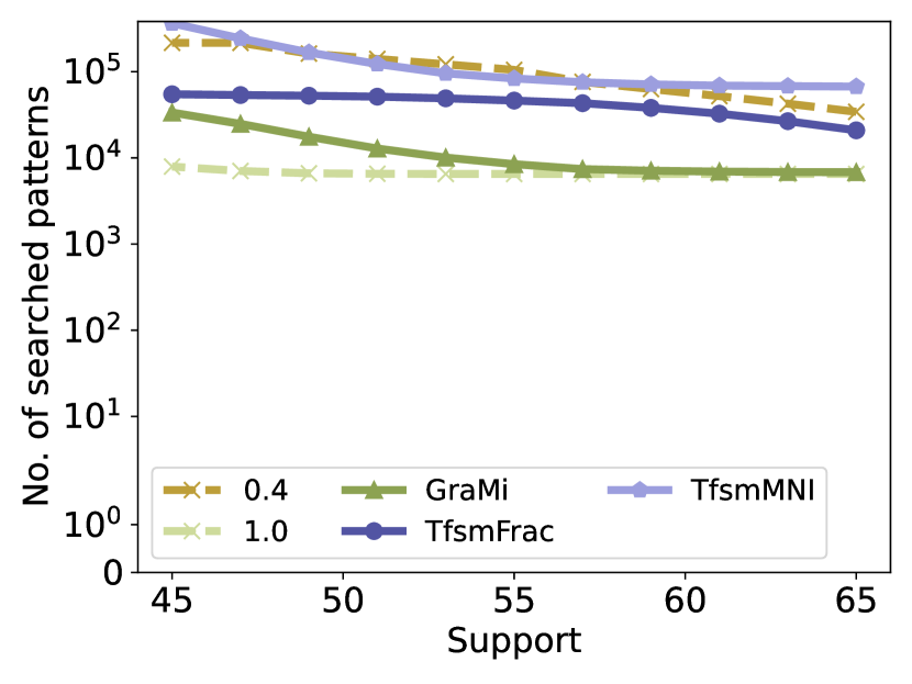
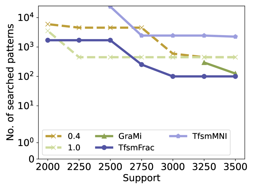
No. of searched patterns for different support values for Gnutella.
for MNI,
for mIS, and
for MNI-Fractional.
T-FSM’s version of MNI is used due to its higher efficiency than GraMi (Yuan et al., 2023)
support
57
75043
34236
43110
59
70910
27022
38035
61
68727
19865
32573
63
67853
13044
26657
65
67025
10431
20879
4.5. Frequent Subgraph Instances
Table 2 shows that we conducted fewer searches when compared to GraMi and T-FSM algorithms, for a value of . The reason we conducted fewer searches is because of our way of choosing which patterns to look for. We focused only on exploring graphs that could be made from the frequent graphs we found earlier. In contrast to GraMi, which spends time looking at all the possible extensions that could come from the frequent graphs in previous steps.
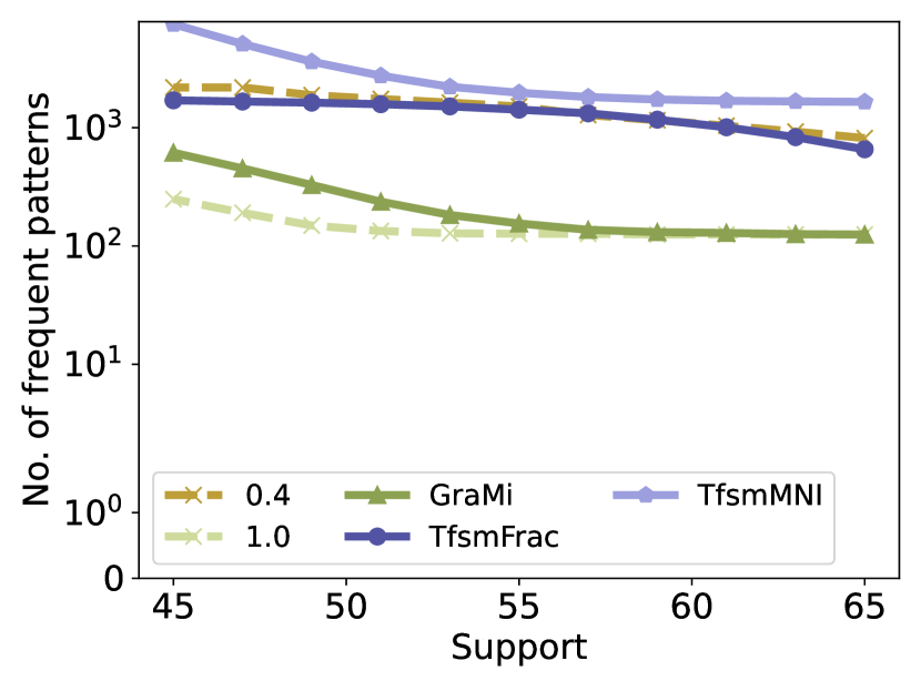
However, FLEXIS searches more candidate patterns as the effective threshold reduces as decreases. Specifically, FLEXIS () searches 7.2x and 5.7x more than GraMi and T-FSM fractional. This might be because, we find more frequent patterns in at when compared to GraMi and T-FSM, as shown in Figures 12(a) and 12(b). Precisely we found 8.8x and 2.4x more than frequent patterns than GraMi and T-FSM. Note as the number of found patterns increases, the number of patterns that can be combined to form a new candidate pattern also increases.
| 1600 | 2 | 125 | 100 | 75 | 100 | 50 |
| 1700 | 2 | 108 | 100 | 75 | 86 | 50 |
4.6. Difference in identified Frequent Patterns
As can be noticed in Table 3, there is not a complete intersection between both, this can be attributed to the following reasons,
-
•
Difference in the approach: Our method uses an undirected data processing and directed matcher method, while GraMi uses fully directed search. So there is a possibility that we are getting some frequent patterns, which GraMi does not find.
-
•
Difference in over-estimation: In lower slider values, mIS tends to over-estimate due to the approximation applied to the threshold value. In contrast, the overestimation of GraMi is due to the recounting of the same vertices, considering automorphism and so on. Thus, the over-estimated patterns might not match between FLEXIS and GraMi.
5. Related Work
The solution to the FSM problem can be largely derived from a two-step process, primarily extended from the work of (Nguyen et al., 2022). The initial step, referred to as the ‘Generation step’, involves the creation of all possible candidate patterns and potential subgraph candidates. Following this, the candidate subgraph space is streamlined by pruned automorphisms. Lastly, the ‘Metric step’ is the number of isomorphic instances among the selected candidates within the data graph, determining whether it exceeds predefined support. Many of the algorithms presented in the context of Subgraph Isomorphism focus on modifying one or more of these components to enhance overall performance.
In the generation step, all possible subgraphs can be achieved through two main methods: edge extension and vertex extension. In the edge extension methods, a candidate subgraph is derived from an existing frequent candidate by adding an edge. This process can be accomplished in two distinct ways. Initially, the path extension approach is employed, where vertices within the frequent subgraph are expanded by adding edges, as illustrated in previous works such as Peregrine, GSpan, Pangolin, and Arabesque (Jamshidi et al., 2020; Yan and Han, 2002; Chen et al., 2020; Teixeira et al., 2015). Alternatively, the utilization of level-wise methods becomes prominent, wherein two frequent subgraphs of order combine to form a subgraph of order (Kuramochi and Karypis, 2005). In the context of vertex extension methods, the frequent subgraphs are expanded by adding a vertex (Chen et al., 2020; Teixeira et al., 2015). Notably, there has been limited exploration into the extension of level-wise notions within the context of vertex extension scenarios. In this paper, we introduce a novel approach that integrates the level-wise methodology into vertex extension methods.
Within the generation step, the redundant and automorphic candidate graphs must be eliminated. The common practice involves the utilization of canonical representations to eliminate redundant candidate graphs that are generated. Diverse canonical representations exist, including the Minimum DFS Code representation (Yan and Han, 2002), Bliss (Junttila and Kaski, 2007b), Eigen Value representations (Zhao et al., 2020), Canonical Adjacency matrix representations, as well as Breadth First Canonical String and Depth First Canonical String representations (Jiang et al., 2013), among others. Given its exceptional efficiency, Bliss is selected as the method of choice in this paper.
The last step of FSM is the ‘Metric’ phase, wherein the generated candidates are compared with the data graphs to ascertain the frequency of occurrence (matches) of a specific candidate within the data graph. This comparison also involves assessing whether the match count exceeds a predefined threshold. Subgraph isomorphism methods are employed for match determination. Varied iterations of this phase exist within the literature. The gold standard is utilizing the Maximum Independent Set (Fiedler and Borgelt, 2007), which identifies the maximal number of disjoint subgraph isomorphisms in the primary graph, an NP-complete problem in itself. An alternative, SATMargin (Liu and Li, 2022), employs random walks, framing the subgraph mining challenge as an SAT problem and employing an SAT algorithm (such as CryptoMiniSat (Soos et al., 2019)) for its resolution. Notably, the most prevailing approximation method is MNI (Bringmann and Nijssen, 2008), which tends to overestimate the number of isomorphic patterns by allowing certain overlaps. MNI finds extensive utilization either directly or with subsequent optimization strategies (Elseidy et al., 2014; Jamshidi et al., 2020; Chen et al., 2020, 2021). In the context of GraMi (Elseidy et al., 2014), graph mining is conceptualized as a Constraint Satisfaction Problem (CSP) that uses MNI to prune the search space. Other metrics that are an extension to MNI, such as a fractional score, which alleviates the over-estimation of MNI have also been proposed (Yuan et al., 2023). While this method succeeds in reducing the overestimation to a limit, it still shows a substantial overestimation. Therefore, this paper introduces an innovative metric termed ’Maximal Independent Set,’ an approximation of the Maximum Independent Set that provides the users with a slider to control the overlap that is required with the Maximum Independent set. While we might also overestimate, it can be brought to the minimum if the user chooses to. Notably, our proposed method diverges from the concepts of maximal frequent subgraph as discussed in SATMargin (Liu and Li, 2022) and Margin (Thomas et al., 2010), wherein the focus is on determining the maximum feasible size of a frequent subgraph, as opposed to utilizing it as a metric, as shown in our study.
While tangential to the core focus of this paper, the subsequent passages are included to provide a definitive categorization of our study.
FSM algorithms can be classified into two distinct categories: 1) Transactional methods, and 2) Single-graph methods. Transactional algorithms (Liu and Li, 2022; Thomas et al., 2010), define a frequent pattern as one that occurs across a set number of graphs. In other words, within a collection of data graphs, a pattern is deemed frequent if it emerges in more than support () data graphs. Conversely, the single graph paradigm considers a pattern frequent if it repeats a predefined number of times within a single large graph (Elseidy et al., 2014; Nguyen et al., 2021; Mawhirter et al., 2021; Jamshidi et al., 2020; Chen et al., 2022). This paper squarely falls within the realm of Single-graph methods. Notably, there exist other methodological extensions within FSM that aim to ascertain precise support counts (Nguyen et al., 2020), solely consider closed-form solutions (Nguyen et al., 2021) or delve into weighted subgraph mining (Le et al., 2020). These extensions, however, lie outside the scope of our current investigation.
Moreover, Subgraph Mining can be achieved through diverse ways, spanning CPU-based approaches (Elseidy et al., 2014; Mawhirter and Wu, 2019; Mawhirter et al., 2021; Aberger et al., 2017; Shi et al., 2020; Jamshidi et al., 2020), GPU-accelerated techniques (Chen et al., 2020; Guo et al., 2020b, a; Chen et al., 2022), Distributed Systems (Salem et al., 2021), near-memory architectures (Dai et al., 2022), and out-of-core systems (Zhao et al., 2020). In this present study, we focus exclusively on CPU-based architectures. However, it is important to note that our proposed method exhibits adaptability for potential extension to GPU and other architectural frameworks.
6. Conclusion
In this paper, we introduce a novel metric based on maximal independent sets (MIS) that enables users to fine-tune the level of overlap they require with the original results. This level of customizability can be invaluable, particularly in applications where precision is paramount. We also proposed an innovative technique for efficiently generating the candidate search space by merging previously identified frequent subgraphs. This approach significantly reduced the computational overhead associated with graph mining, making it more accessible and practical. By incorporating these methods we showed that our method performs better than the existing state-of-art GraMi and T-FSM. In essence, our contributions pave the way for more effective and versatile graph mining techniques, expanding their utility across a wide spectrum of applications.
References
- (1)
- Aberger et al. (2017) Christopher R Aberger, Andrew Lamb, Susan Tu, Andres Nötzli, Kunle Olukotun, and Christopher Ré. 2017. Emptyheaded: A relational engine for graph processing. ACM Transactions on Database Systems (TODS) 42, 4 (2017), 1–44.
- Bindu and Thilagam (2016) PV Bindu and P Santhi Thilagam. 2016. Mining social networks for anomalies: Methods and challenges. Journal of Network and Computer Applications 68 (2016), 213–229.
- Bringmann and Nijssen (2008) Björn Bringmann and Siegfried Nijssen. 2008. What is frequent in a single graph?. In Advances in Knowledge Discovery and Data Mining: 12th Pacific-Asia Conference, PAKDD 2008 Osaka, Japan, May 20-23, 2008 Proceedings 12. Springer, Springer Berlin Heidelberg, Berlin, Heidelberg, 858–863. https://doi.org/10.1007/978-3-540-68125-0_84
- Carletti et al. (2018) Vincenzo Carletti, Pasquale Foggia, Antonio Greco, Alessia Saggese, and Mario Vento. 2018. The VF3-light subgraph isomorphism algorithm: when doing less is more effective. In Structural, Syntactic, and Statistical Pattern Recognition: Joint IAPR International Workshop, S+ SSPR 2018, Beijing, China, August 17–19, 2018, Proceedings 9. Springer, Springer Berlin Heidelberg, Berlin, Heidelberg, 315–325. https://doi.org/10.1007/978-3-319-97785-0_30
- Carletti et al. (2019) Vincenzo Carletti, Pasquale Foggia, Antonio Greco, Mario Vento, and Vincenzo Vigilante. 2019. VF3-Light: a lightweight subgraph isomorphism algorithm and its experimental evaluation. Pattern Recognition Letters 125 (2019), 591–596. https://doi.org/10.1016/j.patrec.2019.07.001
- Chen et al. (2022) Xuhao Chen et al. 2022. Efficient and Scalable Graph Pattern Mining on GPUs. In 16th USENIX Symposium on Operating Systems Design and Implementation (OSDI 22). UNENIX Association, 2560 Ninth St. Suite 215 Berkeley, CA, 857–877.
- Chen et al. (2021) Xuhao Chen, Roshan Dathathri, Gurbinder Gill, Loc Hoang, and Keshav Pingali. 2021. Sandslash: a two-level framework for efficient graph pattern mining. In Proceedings of the ACM International Conference on Supercomputing. ACM, Association for Computing Machinery, New York, NY, USA, 378–391. https://doi.org/10.48550/arXiv.2011.03135
- Chen et al. (2020) Xuhao Chen, Roshan Dathathri, Gurbinder Gill, and Keshav Pingali. 2020. Pangolin: An efficient and flexible graph mining system on cpu and gpu. Proceedings of the VLDB Endowment 13, 8 (2020), 1190–1205.
- Clark and Holton (2005) John Clark and Derek Allan Holton. 2005. A first look at graph theory. World Scientific, Singapore.
- Dai et al. (2022) Guohao Dai, Zhenhua Zhu, Tianyu Fu, Chiyue Wei, Bangyan Wang, Xiangyu Li, Yuan Xie, Huazhong Yang, and Yu Wang. 2022. Dimmining: pruning-efficient and parallel graph mining on near-memory-computing. In Proceedings of the 49th Annual International Symposium on Computer Architecture. Association for Computing Machinery, New York, NY, USA, 130–145. https://doi.org/10.1145/3470496.3527388
- Elseidy et al. (2014) Mohammed Elseidy, Ehab Abdelhamid, Spiros Skiadopoulos, and Panos Kalnis. 2014. Grami: Frequent subgraph and pattern mining in a single large graph. Proceedings of the VLDB Endowment 7, 7 (2014), 517–528. https://doi.org/10.14778/2732286.2732289
- Fiedler and Borgelt (2007) Mathias Fiedler and Christian Borgelt. 2007. Support computation for mining frequent subgraphs in a single graph. In MLG. Association for Computing Machinery, New York, NY, USA.
- Guo et al. (2020b) Wentian Guo, Yuchen Li, Mo Sha, Bingsheng He, Xiaokui Xiao, and Kian-Lee Tan. 2020b. Gpu-accelerated subgraph enumeration on partitioned graphs. In Proceedings of the 2020 ACM SIGMOD International Conference on Management of Data. Association for Computing Machinery, New York, NY, USA, 1067–1082.
- Guo et al. (2020a) Wentian Guo, Yuchen Li, and Kian-Lee Tan. 2020a. Exploiting reuse for GPU subgraph enumeration. IEEE Transactions on Knowledge and Data Engineering 34, 9 (2020), 4231–4244.
- Jamshidi et al. (2020) Kasra Jamshidi, Rakesh Mahadasa, and Keval Vora. 2020. Peregrine: a pattern-aware graph mining system. In Proceedings of the Fifteenth European Conference on Computer Systems. Association for Computing Machinery, New York, NY, USA, 1–16. https://doi.org/10.48550/arXiv.2004.02369
- Jiang et al. (2013) Chuntao Jiang, Frans Coenen, and Michele Zito. 2013. A survey of frequent subgraph mining algorithms. The Knowledge Engineering Review 28, 1 (2013), 75–105. https://doi.org/10.1017/S0269888912000331
- Junttila and Kaski (2007a) Tommi Junttila and Petteri Kaski. 2007a. Engineering an efficient canonical labeling tool for large and sparse graphs. In Proceedings of the Ninth Workshop on Algorithm Engineering and Experiments and the Fourth Workshop on Analytic Algorithms and Combinatorics, David Applegate, Gerth Stølting Brodal, Daniel Panario, and Robert Sedgewick (Eds.). SIAM, Philadelphia, 135–149. https://doi.org/10.1137/1.9781611972870.13
- Junttila and Kaski (2007b) Tommi Junttila and Petteri Kaski. 2007b. Engineering an efficient canonical labeling tool for large and sparse graphs. In 2007 Proceedings of the Ninth Workshop on Algorithm Engineering and Experiments (ALENEX). SIAM, Society for Industrial and Applied Mathematics, Philadelphia, Pennsylvania, 135–149. https://doi.org/10.5555/2791188.2791201
- Junttila and Kaski (2011) Tommi Junttila and Petteri Kaski. 2011. Conflict Propagation and Component Recursion for Canonical Labeling. In Theory and Practice of Algorithms in (Computer) Systems – First International ICST Conference, TAPAS 2011, Rome, Italy, April 18–20, 2011. Proceedings (Lecture Notes in Computer Science), Alberto Marchetti-Spaccamela and Michael Segal (Eds.), Vol. 6595. Springer, Berlin, Heidelberg, 151–162. https://doi.org/10.1007/978-3-642-19754-3_16
- Kingan (2022) Sandra R. Kingan. 2022. Graphs and Networks. Wiley, Hoboken, NJ.
- Kong et al. (2022) Xiangzhe Kong, Wenbing Huang, Zhixing Tan, and Yang Liu. 2022. Molecule generation by principal subgraph mining and assembling. Advances in Neural Information Processing Systems 35 (2022), 2550–2563.
- Kuramochi and Karypis (2004) M. Kuramochi and G. Karypis. 2004. An efficient algorithm for discovering frequent subgraphs. IEEE Transactions on Knowledge and Data Engineering 16, 9 (2004), 1038–1051. https://doi.org/10.1109/TKDE.2004.33
- Kuramochi and Karypis (2005) Michihiro Kuramochi and George Karypis. 2005. Finding frequent patterns in a large sparse graph. Data mining and knowledge discovery 11, 3 (2005), 243–271. https://doi.org/10.1007/s10618-005-0003-9
- Le et al. (2020) Ngoc-Thao Le, Bay Vo, Lam BQ Nguyen, Hamido Fujita, and Bac Le. 2020. Mining weighted subgraphs in a single large graph. Information Sciences 514 (2020), 149–165. https://doi.org/10.1016/j.ins.2019.12.010
- Leskovec et al. (2010a) Jure Leskovec, Daniel Huttenlocher, and Jon Kleinberg. 2010a. Predicting positive and negative links in online social networks. In Proceedings of the 19th international conference on World wide web. Association for Computing Machinery, New York, NY, USA, 641–650.
- Leskovec et al. (2010b) Jure Leskovec, Daniel Huttenlocher, and Jon Kleinberg. 2010b. Signed networks in social media. In Proceedings of the SIGCHI conference on human factors in computing systems. Association for Computing Machinery, New York, NY, USA, 1361–1370.
- Leskovec et al. (2007) Jure Leskovec, Jon Kleinberg, and Christos Faloutsos. 2007. Graph evolution: Densification and shrinking diameters. ACM transactions on Knowledge Discovery from Data (TKDD) 1, 1 (2007), 2–es.
- Leskovec et al. (2009) Jure Leskovec, Kevin J Lang, Anirban Dasgupta, and Michael W Mahoney. 2009. Community structure in large networks: Natural cluster sizes and the absence of large well-defined clusters. Internet Mathematics 6, 1 (2009), 29–123.
- Liu and Li (2022) Muyi Liu and Pan Li. 2022. SATMargin: Practical Maximal Frequent Subgraph Mining via Margin Space Sampling. In Proceedings of the ACM Web Conference 2022. ACM, Association for Computing Machinery, New York, NY, USA, 1495–1505. https://doi.org/10.1145/3485447.3512196
- Martinelli et al. (2013) Fabio Martinelli, Andrea Saracino, and Daniele Sgandurra. 2013. Classifying android malware through subgraph mining. In International Workshop on Data Privacy Management. Springer, Berlin, Heidelberg, 268–283.
- Mawhirter et al. (2021) Daniel Mawhirter, Sam Reinehr, Connor Holmes, Tongping Liu, and Bo Wu. 2021. Graphzero: A high-performance subgraph matching system. ACM SIGOPS Operating Systems Review 55, 1 (2021), 21–37.
- Mawhirter and Wu (2019) Daniel Mawhirter and Bo Wu. 2019. Automine: harmonizing high-level abstraction and high performance for graph mining. In Proceedings of the 27th ACM Symposium on Operating Systems Principles. Association for Computing Machinery, New York, NY, USA, 509–523.
- Mrzic et al. (2018) Aida Mrzic, Pieter Meysman, Wout Bittremieux, Pieter Moris, Boris Cule, Bart Goethals, and Kris Laukens. 2018. Grasping frequent subgraph mining for bioinformatics applications. BioData mining 11, 1 (2018), 1–24.
- Nguyen et al. (2021) Lam BQ Nguyen, Loan TT Nguyen, Ivan Zelinka, Vaclav Snasel, Hung Son Nguyen, and Bay Vo. 2021. A method for closed frequent subgraph mining in a single large graph. IEEE Access 9 (2021), 165719–165733. https://doi.org/10.1109/ACCESS.2021.3133666
- Nguyen et al. (2020) Lam BQ Nguyen, Bay Vo, Ngoc-Thao Le, Vaclav Snasel, and Ivan Zelinka. 2020. Fast and scalable algorithms for mining subgraphs in a single large graph. Engineering Applications of Artificial Intelligence 90 (2020), 103539. https://doi.org/10.1016/j.engappai.2020.103539
- Nguyen et al. (2022) Lam BQ Nguyen, Ivan Zelinka, Vaclav Snasel, Loan TT Nguyen, and Bay Vo. 2022. Subgraph mining in a large graph: A review. Wiley Interdisciplinary Reviews: Data Mining and Knowledge Discovery 12, 4 (2022), e1454.
- Richardson et al. (2003) Matthew Richardson, Rakesh Agrawal, and Pedro Domingos. 2003. Trust management for the semantic web. In International semantic Web conference. Springer, Springer Berlin Heidelberg, Berlin, Heidelberg, 351–368.
- RIPEANU et al. (2002) Matei RIPEANU, Adriana IAMNITCHI, and Ian FOSTER. 2002. Mapping the Gnutella network. IEEE internet computing 6, 1 (2002), 50–57.
- Salem et al. (2021) Saeed Salem, Mohammed Alokshiya, and Mohammad Al Hasan. 2021. RASMA: a reverse search algorithm for mining maximal frequent subgraphs. BioData Mining 14 (2021), 1–23.
- Shi et al. (2020) Tianhui Shi, Mingshu Zhai, Yi Xu, and Jidong Zhai. 2020. Graphpi: High performance graph pattern matching through effective redundancy elimination. In SC20: International Conference for High Performance Computing, Networking, Storage and Analysis. IEEE, Insitute of Electrical and Electronics Engineers, Piscataway, NJ, USA, 1–14.
- Soos et al. (2019) Mate Soos, Armin Biere, M Heule, M Jarvisalo, and M Suda. 2019. CryptoMiniSat 5.6 with YalSAT at the SAT Race 2019. Proc. of SAT Race B-2019-1 (2019), 14–15.
- Teixeira et al. (2015) Carlos HC Teixeira, Alexandre J Fonseca, Marco Serafini, Georgos Siganos, Mohammed J Zaki, and Ashraf Aboulnaga. 2015. Arabesque: a system for distributed graph mining. In Proceedings of the 25th Symposium on Operating Systems Principles. Association for Computing Machinery, New York, NY, USA, 425–440.
- Thomas et al. (2010) Lini T Thomas, Satyanarayana R Valluri, and Kamalakar Karlapalem. 2010. Margin: Maximal frequent subgraph mining. ACM Transactions on Knowledge Discovery from Data (TKDD) 4, 3 (2010), 1–42. https://doi.org/10.1145/1839490.1839491
- Yan and Han (2002) Xifeng Yan and Jiawei Han. 2002. gspan: Graph-based substructure pattern mining. In 2002 IEEE International Conference on Data Mining, 2002. Proceedings. IEEE, Institute of Electrical and Electronics Engineers, Piscataway, NJ, USA, 721–724. https://doi.org/10.1109/ICDM.2002.1184038
- Yao et al. (2020) Pengcheng Yao, Long Zheng, Zhen Zeng, Yu Huang, Chuangyi Gui, Xiaofei Liao, Hai Jin, and Jingling Xue. 2020. A locality-aware energy-efficient accelerator for graph mining applications. In 2020 53rd Annual IEEE/ACM International Symposium on Microarchitecture (MICRO). IEEE, Institute of Electrical and Electronics Engineers, Piscataway, NJ, USA, 895–907.
- Yuan et al. (2023) Lyuheng Yuan, Da Yan, Wenwen Qu, Saugat Adhikari, Jalal Khalil, Cheng Long, and Xiaoling Wang. 2023. T-FSM: A Task-Based System for Massively Parallel Frequent Subgraph Pattern Mining from a Big Graph. Proc. ACM Manag. Data 1, 1, Article 74 (may 2023), 26 pages. https://doi.org/10.1145/3588928
- Zhao et al. (2020) Cheng Zhao, Zhibin Zhang, Peng Xu, Tianqi Zheng, and Jiafeng Guo. 2020. Kaleido: An efficient out-of-core graph mining system on A single machine. In 2020 IEEE 36th International Conference on Data Engineering (ICDE). IEEE, Insitute of Electrical and Electronics Engineers, Piscataway, NJ, USA, 673–684.