Burning Random Trees

Abstract

Let $\mathcal{T}$ be a Galton-Watson tree with a given offspring distribution $\xi$, where $\xi$ is a $\mathbb{Z}_{\geq 0}$-valued random variable with $\textsf{E}[\xi]=1$ and $0<\sigma^{2}:=\textsf{Var}[\xi]<\infty$. For $n\geq 1$, let $T_{n}$ be the tree $\mathcal{T}$ conditioned to have $n$ vertices. In this paper we investigate $b(T_{n})$, the burning number of $T_{n}$. Our main result shows that asymptotically almost surely $b(T_{n})$ is of the order of $n^{1/3}$.

1 Introduction

Graph burning is a discrete-time process that models influence spreading in a network. Vertices are in one of two states: either burning or unburned. In each round, a burning vertex causes all of its neighbours to burn and a new fire source is chosen: a previously unburned vertex whose state is changed to burning. The updates repeat until all vertices are burning. The burning number of a graph $G$, denoted $b(G)$, is the minimum number of rounds required to burn all of the vertices of $G$.

Graph burning first appeared in print in a paper of Alon [2], motivated by a question of Brandenburg and Scott at Intel, and was formulated as a transmission problem involving a set of processors. It was then independently studied by Bonato, Janssen, and Roshanbin [5, 6] who, in addition to introducing the name graph burning, gave bounds and characterized the burning number for various graph classes. The problem has since received wide attention (e.g. [3, 4, 11, 14, 15, 16]), with particular focus the so-called Burning Number Conjecture that each connected graph on $n$ vertices requires at most $\lceil\sqrt{n}\rceil$ turns to burn. This conjecture is best possible, as $b(P_{n})=\left\lceil\sqrt{n}\right\rceil$ for a path on $n$ vertices.

Clearly, $b(G)\leq b(T)$ for every spanning tree $T$ of $G$. Hence, the Burning Number Conjecture can be stated as follows:

Conjecture 1.1.

For any tree $T$ on $n$ vertices, $b(T)\leq\left\lceil\sqrt{n}\right\rceil$.

Although the conjecture feels obvious, it has resisted attempts at its resolution. It is easy to couple the process on any tree $T$ on $n$ vertices ($n-1$ edges) with the process on $C_{2(n-1)}$, a cycle on twice as many edges. (See Figure 1.) This yields

$$b(T)\leq\left\lceil\sqrt{2(n-1)}\right\rceil=\sqrt{2n}+O(1)\qquad(\sqrt{2}\approx 1.41421).$$

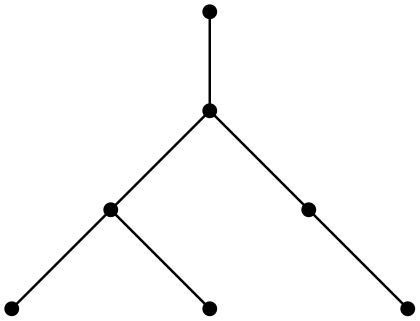
(a)

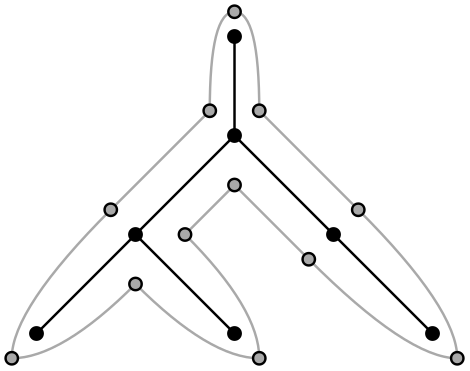
(b)

Figure 1: A tree $T$ (a) and a cycle corresponding to a depth-first search of $T$ (b). Any burning sequence for the cycle projects to a burning sequence for the tree.

In [4], it was proved that

$$b(T)\leq\sqrt{\frac{12}{7}n}+3\qquad(\sqrt{12/7}\approx 1.30931).$$

This bound was consecutively improved in [11] to

$$b(T)\leq\left\lceil\frac{\sqrt{24n+33}-3}{4}\right\rceil=\sqrt{\frac{3}{2}\,n}+O(1)\qquad(\sqrt{3/2}\approx 1.22475),$$

and currently, the best upper bound proved in [3], is

$$b(T)\leq\left\lceil\sqrt{\frac{4}{3}n}\right\rceil+1\qquad(\sqrt{4/3}\approx 1.15470).$$

Arguably, the strongest result in this direction shows that the conjecture holds asymptotically [16], that is,

$$b(T)\leq(1+o(1))\sqrt{n}.$$

We intend to investigate the burning number of random trees. Let $\mathcal{T}$ be a Galton-Watson tree with a given offspring distribution $\xi$, where $\xi$ is a $\mathbb{Z}_{\geq 0}$-valued random variable with

$$\textsf{E}[\xi]=1,\qquad\text{ and }\qquad 0<\sigma^{2}:=\textsf{Var}[\xi]<\infty.$$ (1)

In other words, the Galton-Watson tree is critical, of finite variance, and satisfies $\mathbb{P}(\xi=1)<1$. In particular, it implies that $0<\mathbb{P}(\xi=0)<1$.

For $n\geq 1$, let $T_{n}$ be the tree $\mathcal{T}$ conditioned to have $n$ vertices. The resulting random trees are essentially the same as the simply generated families of trees introduced by Meir and Moon [13]. This family contains many combinatorially interesting random trees such as uniformly chosen random plane trees, random unordered labelled trees (known as Cayley trees), and random $d$-ary trees. For more examples, see, Aldous [1] and Devroye [7].

Our main result shows that, with high probability, $b(T_{n})$ is of the order of $n^{1/3}$.

Theorem 1.2.

Let $T_{n}$ be a conditioned Galton-Watson tree of order $n$, subject to (1). For any $\epsilon=\epsilon(n)$ tending to $0$ as $n\to\infty$, we have

$$\textsf{Pr}\Big{(}(\epsilon n)^{1/3}\leq b(T_{n})\leq(n/\epsilon)^{1/3}\Big{)}=1-O(\epsilon).$$

The paper is structured as follows. First, we make a simple observation that the burning number can be reduced to the problem of covering vertices of the graph with balls, a slightly easier problem; see Section 2. Section 3 is devoted to the lower bound for the burning number whereas the upper bound is provided in Section 4. We finish the paper with a few natural questions; see Section 5.

2 Covering a Graph with Balls

In this section, we show a simple but convenient observation that reduces the burning number to the problem of covering the graph’s vertices with balls. Let $G=(V,E)$ be any graph. For any $r\in{\mathbb{N}}_{0}$ and vertex $v\in V$, we denote by $B_{r}(v)$ the ball of radius $r$ centered at $v$, that is, $B_{r}(v)=\{u\in V:d(u,v)\leq r\}$, where $d(u,v)$ denotes the distance between $u$ and $v$.

First, note that since the burning process is deterministic, a fire source $v$ makes all vertices in $B_{t}(v)$ burn after $t$ rounds but only those vertices are affected. As a result, the burning number can be reformulated as follows:

$$b(G)=\min\left\{k\in{\mathbb{N}}:\exists v_{0},v_{1},\ldots,v_{k-1}\in V\text{ such that }\bigcup_{r=0}^{k-1}B_{r}(v_{r})=V\right\}.$$

Dealing with balls of different radii is inconvenient so we will simplify the problem slightly by considering balls of the same radii. Let $\hat{b}(G)$ be the counterpart of $b(G)$ for this auxiliary covering problem, that is,

$$\hat{b}(G)=\min\left\{k\in{\mathbb{N}}:\exists v_{1},v_{2},\ldots,v_{k}\in V\text{ such that }\bigcup_{r=1}^{k}B_{k}(v_{r})=V\right\}.$$

Covering with $k$ balls of increasing radii (in particular, all of them of radii at most $k-1$) is not easier than covering with $k$ balls of radius $k$. Hence, $\hat{b}(G)\leq b(G)$. On the other hand, covering with $2k$ balls of increasing radii (in particular, $k$ of them of radii at least $k$) is not more difficult than covering with $k$ balls of radius $k$ implying that $b(G)\leq 2\hat{b}(G)$. We conclude that $\hat{b}(G)$ and $b(G)$ are of the same order:

Observation 2.1.

For any graph $G=(V,E)$,

$$\hat{b}(G)\leq b(G)\leq 2\hat{b}(G).$$

In particular, we may prove the bounds in our main result (Theorem 1.2) for $\hat{b}(G)$ instead of $b(G)$, which will be slightly easier.

3 Lower bound

For an arbitrary tree $\tau$ and $i\in{\mathbb{N}}$, let

$$P_{i}(\tau):=\left|\Big{\{}\{v,w\}:v,w\in V(\tau),\,d(v,w)=i\Big{\}}\right|.$$

In other words, $P_{i}(\tau)$ counts the number of unordered pairs of vertices which are distance $i$ apart in $\tau.$ We have the following result from [8] that upper bounds the expected number of such pairs in the random tree $T_{n}$:

Theorem 3.1 ([8, Theorem 1.3]).

There exists a constant $c>0$, dependent on the distribution of $\xi$, such that for all $n\in{\mathbb{N}}$ and $i\in{\mathbb{N}}$, $\textsf{E}[P_{i}(T_{n})]\leq cni$.

We use Theorem 3.1 to prove the following:

Proposition 3.2.

Let $k=k(n)=(\epsilon n)^{1/3}$, where $\epsilon=\epsilon(n)\to 0$ as $n\to\infty$. With probability $1-O(\epsilon)$, $\hat{b}(T_{n})\geq k$, that is, there is no partition of the vertices of $T_{n}$ into $k$ disjoint sets $U_{1},U_{2},\dots,U_{k}$ such that $\text{diam}(U_{j})\leq 2k$ for all $1\leq j\leq k$.

Since $b(T_{n})\geq\hat{b}(T_{n})$ (Observation 2.1), Proposition 3.2 implies the corresponding lower bound in Theorem 1.2.

Proof.

Let $Q_{j}(T_{n})=\sum_{i=1}^{j}P_{i}(T_{n})$, that is, $Q_{j}(T_{n})$ counts pairs of vertices in $T_{n}$ which are at most distance $j$ apart. From Theorem 3.1, for all $n,j\in{\mathbb{N}}$,

$$\textsf{E}[Q_{j}(T_{n})]=\sum_{i=1}^{j}\textsf{E}[P_{i}(T_{n})]\leq cn\sum_{i=1}^{j}i\leq cnj^{2}.$$

For a contradiction, suppose there is a partition $U_{1},U_{2},\dots,U_{k}$ of the vertices of $T_{n}$ as described in the statement of the proposition. Since every pair of vertices in a given $U_{j}$ is at most distance $2k$ apart, we must have

$$Q_{2k}(T_{n})\geq\sum_{j=1}^{k}\binom{|U_{j}|}{2}=\sum_{j=1}^{k}\left(\frac{|U_{j}|^{2}}{2}-\frac{|U_{j}|}{2}\right)=\frac{1}{2}\sum_{j=1}^{k}|U_{j}|^{2}-\frac{n}{2}.$$

By Jensen’s inequality, we get

$$\frac{1}{k}\sum_{j=1}^{k}|U_{j}|^{2}\geq\left(\frac{1}{k}\sum_{j=1}^{k}|U_{j}|\right)^{2}=\left(\frac{n}{k}\right)^{2}$$

and therefore

$$Q_{2k}(T_{n})\geq\frac{n^{2}}{2k}-\frac{n}{2}=\frac{n^{2}}{2k}\left(1-O(k/n)\right)=\frac{n^{2}}{2k}\left(1-o(n^{-2/3})\right).$$

On the other hand, $\textsf{E}[Q_{2k}(T_{n})]\leq 4cnk^{2}$. Thus, by Markov’s inequality,

$$\textsf{Pr}\left(Q_{2k}(T_{n})\geq\frac{n^{2}}{2k}-\frac{n}{2}\right) \leq \frac{\textsf{E}[Q_{2k}(T_{n})]}{\frac{n^{2}}{2k}}\left(1+o(n^{-2/3})\right)$$

$$= O\left(\frac{k^{3}}{n}\right)=O(\epsilon).$$

It follows that a partition of $V(T_{n})$ with the stated properties exists with probability $O(\epsilon)$, which finishes the proof of the proposition. ∎

4 Upper bound

For any rooted tree $\tau$ with root $r$, for $i\in{\mathbb{N}}_{0}$ we write $\ell_{i}(\tau):=\{v\in V(\tau)\,:\,d_{\tau}(r,v)=i\}$ for the set of vertices at depth $i$. Let $h(\tau)\in{\mathbb{N}}_{0}\cup\{\infty\}$ be the height of $\tau$, that is, $h(\tau):=\sup\{i\,:\,\ell_{i}(\tau)\neq\emptyset\}$. For any $v\in V(\tau)$, let $\tau_{v}$ the (full) sub-tree of $\tau$ rooted at $v$. For $k\in{\mathbb{N}}$, and $j\in\{0,1,\dots,k-1\}$, let

$$\mathcal{C}_{k}^{j}(\tau):=\bigcup_{i=0}^{\infty}\Big{\{}v\in\ell_{ik+j}(\tau)\,:\,h(\tau_{v})\geq k\Big{\}}.$$

So $\mathcal{C}_{k}^{j}(\tau)$ consists of all vertices whose depth is $j$ modulo $k$ with subtrees of height at least $k$.

We first show that placing balls of radius $2k$ at the root and at each vertex in $\mathcal{C}_{k}^{j}(\tau)$ covers the vertices of $\tau$.

Lemma 4.1.

Let $\tau$ be a tree rooted at $r$. For any $k\in{\mathbb{N}}$ and $j\in\{0,1,\dots,k-1\}$ we have

$$V(\tau)=\bigcup_{v\in\mathcal{C}_{k}^{j}(\tau)\cup\{r\}}B_{2k}(v).$$

Proof.

Fix $k\in{\mathbb{N}}$ and $j\in\{0,1,\dots,k-1\}$. Let $v\in V(\tau)$ and let $i$ be the smallest non-negative integer such that $d(r,v)<ik+j$ and let $a$ be the unique ancestor of $v$ in $\ell_{(i-2)k+j}(\tau)$, or $a=r$ if $i\in\{0,1\}$. Then $a$ is either the root $r$, or $d(r,a)\equiv j\pmod{k}$ and $h(\tau_{a})\geq k$. In either case, $a\in\mathcal{C}_{k}^{j}(\tau)\cup\{r\}$. Since $d(a,v)\leq 2k$, we have $v\in B_{2k}(a).$ This finishes the proof of the lemma. ∎

Lemma 4.1 provides a scheme to cover a general rooted tree $\tau$ with balls of radius $2k$. Observe that for any $j$, $|\mathcal{C}_{k}^{j}(\tau)|\leq 2k-1$ implies that $\hat{b}(\tau)\leq 2k$, and hence $b(\tau)\leq 4k$ by Observation 2.1. In particular, we conclude the following:

$$\text{if }\min_{j}|\mathcal{C}_{k}^{j}(\tau)|\leq 2k-1,\text{ then }b(\tau)\leq 4k.$$ (2)

Our next lemma estimates the probability that a vertex selected uniformly at random from the random tree $T_{n}$ has height at least $k$.

Lemma 4.2.

Consider the random tree $\tau=T_{n}$ on $n$ vertices. Then there exists a constant $c>0$, dependent on the distribution of $\xi$, such that the following property holds. Let $u$ be a vertex selected uniformly at random from $V(\tau)$, and let its subtree be denoted by $\tau_{u}$. Then, for all $k\geq 0$,

$$\textsf{Pr}\Big{(}h(\tau_{u})\geq k\Big{)}\leq c\left(\frac{1}{k}+\frac{1}{\sqrt{n}}\right).$$

To prove Lemma 4.2 we require some standard tools for conditioned Galton Watson trees, which we introduce now. Given a tree $\tau$ with $s$ vertices, let $v_{1},v_{2},\dots,v_{s}$ be the vertices of $\tau$ in depth-first search (dfs) order. We write $d_{i}$ for the number of children of $v_{i}$ and refer to $(d_{1},d_{2},\dots,d_{s})$ as the preorder degree sequence of $\tau$. The preorder degree sequence gives rise to a representation of $\tau$ as a lattice path $(j,y_{j})_{j=0}^{s}$ started from $(0,y_{0})=(0,0)$ with $s$ steps, where the $j$th step is given by $y_{j}=y_{j-1}+(d_{j}-1)$. See Figure 2 for an example.

(a)

(b)

Figure 2: A rooted tree $\tau$ with preorder degree sequence $(1,2,2,0,0,1,0)$ (a) and its lattice path representation (b).

Note that the lattice path corresponding to a tree with $s$ vertices always ends at the point $(s,y_{s})=(s,-1)$ and has a height strictly greater than $-1$ before then, evidenced by the fact that the height of the path at step $j$ is one less than the number of vertices in the “queue” of the dfs of the tree after $j$ vertices have been explored. As the next lemma summarizes, there is a bijective correspondence between ordered trees with $s$ vertices and lattice paths of this type.

Lemma 4.3 ([9, Lemma 15.2]).

A sequence $(d_{1},d_{2},\dots,d_{s})\in{\mathbb{N}}_{0}^{s}$ is the preorder degree sequence of a tree if and only if

$$\sum_{i=1}^{j}d_{i}\geq j\quad\forall\,j\in\{1,2,\dots,s-1\}$$

and

$$\sum_{i=1}^{s}d_{j}=s-1.$$

We also have the following useful property.

Lemma 4.4 ([9, Corollary 15.4]).

If $(d_{1},d_{2},\dots,d_{s})\in{\mathbb{N}}_{0}^{s}$ satisfies $\sum_{i=1}^{s}d_{i}=s-1$, then precisely one of the cyclic permutations of $(d_{1},d_{2},\dots,d_{s})$ is the preorder degree sequence of a tree.

Let $(\xi_{1}^{(s)},\xi_{2}^{(s)},\dots,\xi_{s}^{(s)})$ be the preorder degree sequence of a Galton-Watson tree $T_{s}$ with offspring distribution $\xi$ conditioned to have $s$ vertices, and let $(\widetilde{\xi}_{1}^{(s)},\widetilde{\xi}_{2}^{(s)},\dots,\widetilde{\xi}_{s}^{(s)})$ be a uniformly random cyclic permutation of $(\xi_{1}^{(s)},\xi_{2}^{(s)},\dots,\xi_{s}^{(s)})$. Let $\xi_{1},\xi_{2},\dots$ be a sequence of i.i.d. copies of $\xi$, and define, for any $j\geq 1$, $S_{j}=\sum_{i=1}^{j}\xi_{i}$. Lemmas 4.3 and 4.4 yield the following corollary:

Corollary 4.5.

The sequence $(\widetilde{\xi}_{1}^{(s)},\widetilde{\xi}_{2}^{(s)},\dots,\widetilde{\xi}_{s}^{(s)})$ has the same distribution as the sequence $(\xi_{1},\xi_{2},\dots,\xi_{s})$ conditioned on $S_{s}=s-1$.

Define the span of $\xi$ as

$$h=\gcd\{i\geq 1\,:\,\textsf{Pr}(\xi=i)>0\}.$$

We will use the following local limit theorems (see [10, Lemma 4.1 and (4.3)] and the sources referenced therein).

Lemma 4.6.

Suppose $\xi$ satisfies (1) and has span $h$. Then, as $s\to\infty$, uniformly for $m\equiv 0\pmod{h}$,

$$\textsf{Pr}(S_{s}=m)=\frac{h}{\sqrt{2\pi\sigma^{2}s}}\left(e^{-(m-s)^{2}/2s\sigma^{2}}+o(1)\right).$$

If $\mathcal{T}$ is the Galton-Watson tree with offspring distribution $\xi$, then for $s\equiv 1\pmod{h}$, as $s\to\infty$,

$$\textsf{Pr}(|\mathcal{T}|=s)=\frac{h}{\sqrt{2\pi\sigma^{2}s^{3}}}(1+o(1)).$$

We are now ready to prove Lemma 4.2.

Proof of Lemma 4.2.

Throughout the proof, we will use $c_{1},c_{2},\dots$ for non-explicit positive constants which do not depend on $n$ (but may depend on the distribution of $\xi$). Implicitly, we will assume throughout that $n\equiv 1\pmod{h}$, where $h$ is the span of $\xi$, so that $\textsf{Pr}(S_{n}=n-1)>0.$

We identify the random vertex $u$ with a random index of the dfs order on $T_{n}$. Consider $(\xi_{u}^{(n)},\xi_{u+1}^{(n)},\dots,\xi_{n}^{(n)},\xi_{1}^{(n)},\dots,\xi_{u-1}^{(n)}).$ It is clear that this sequence has the same distribution as $(\widetilde{\xi}_{1}^{(n)},\widetilde{\xi}_{2}^{(n)},\dots,\widetilde{\xi}_{n}^{(n)})$, which, in turn, has the same distribution as $(\xi_{1},\xi_{2},\dots,\xi_{n})$ conditioned on $S_{n}=n-1$ by Corollary 4.5.

For $k\in{\mathbb{N}}$ and $s\geq k$, let $\mathfrak{T}_{s}^{k}$ be the set of ordered trees with $s$ vertices and height at least $k$. For a sequence $(d_{1},d_{2},\dots,d_{s})\in{\mathbb{N}}_{0}^{s}$, we write $(d_{1},d_{2},\dots,d_{s})\in\mathfrak{T}_{s}^{k}$ if $(d_{1},d_{2},\dots,d_{s})$ is the preorder degree sequence of a tree in $\mathfrak{T}_{s}^{k}$. Note that for any $(d_{1},d_{2},\dots,d_{s})\in\mathfrak{T}_{s}^{k}$, we have $\sum_{i=1}^{s}d_{i}=s-1$. Then,

$$\textsf{Pr}(h(\tau_{u})\geq k) = \sum_{s=k}^{n}\textsf{Pr}((\widetilde{\xi}_{1}^{(n)},\widetilde{\xi}_{2}^{(n)},\dots,\widetilde{\xi}_{s}^{(n)})\in\mathfrak{T}_{s}^{k})$$ (3)

$$= \sum_{s=k}^{n}\textsf{Pr}((\xi_{1},\xi_{2},\dots,\xi_{s})\in\mathfrak{T}_{s}^{k}\,|\,S_{n}=n-1)$$

$$= \sum_{s=k}^{n}\frac{\textsf{Pr}((\xi_{1},\xi_{2},\dots,\xi_{s})\in\mathfrak{T}_{s}^{k},\,S_{n}=n-1)}{\textsf{Pr}(S_{n}=n-1)}$$

$$= \sum_{s=k}^{n}\frac{\textsf{Pr}((\xi_{1},\xi_{2},\dots,\xi_{s})\in\mathfrak{T}_{s}^{k})\cdot\textsf{Pr}\left(\sum_{i=s+1}^{n}\xi_{i}=n-s\right)}{\textsf{Pr}(S_{n}=n-1)}$$

$$= \sum_{s=k}^{n}\frac{\textsf{Pr}((\xi_{1},\xi_{2},\dots,\xi_{s})\in\mathfrak{T}_{s}^{k})\cdot\textsf{Pr}(S_{n-s}=n-s)}{\textsf{Pr}(S_{n}=n-1)}.$$

By Lemma 4.6, there is a constant $c_{1}>0$ such that for $s\in\{1,2,\dots,\lfloor n/2\rfloor\}$, we have

$$\frac{\textsf{Pr}(S_{n-s}=n-s)}{\textsf{Pr}(S_{n}=n-1)}\leq c_{1}.$$

Thus,

$$\sum_{s=k}^{\lfloor n/2\rfloor}\frac{\textsf{Pr}((\xi_{1},\xi_{2},\dots,\xi_{s})\in\mathfrak{T}_{s}^{k})\cdot\textsf{Pr}(S_{n-s}=n-s)}{\textsf{Pr}(S_{n}=n-1)} \leq c_{1}\sum_{s=k}^{\lfloor n/2\rfloor}\textsf{Pr}((\xi_{1},\xi_{2},\dots,\xi_{s})\in\mathfrak{T}_{s}^{k})$$

$$\leq c_{1}\sum_{s=k}^{\infty}\textsf{Pr}((\xi_{1},\xi_{2},\dots,\xi_{s})\in\mathfrak{T}_{s}^{k})$$

$$= c_{1}\,\textsf{Pr}(h(\mathcal{T})\geq k),$$

where, recall, $\mathcal{T}$ is the unconditioned Galton-Watson tree with offspring distribution $\xi$. By Kolmogorov’s Theorem [12, Theorem 12.7], there is a constant $c_{2}>0$ so that for any $k\geq 1$, we have $\textsf{Pr}(h(\mathcal{T})\geq k)\leq c_{2}/k$, and thus $c_{1}\,\textsf{Pr}(h(\mathcal{T})\geq k)\leq c_{3}/k$ for some constant $c_{3}>0$. This bounds the partial sum of (3) where $k\leq s\leq n/2$.

For the other partial sum, we first observe that

$$\textsf{Pr}((\xi_{1},\xi_{2},\dots,\xi_{s})\in\mathfrak{T}_{s}^{k})\leq\textsf{Pr}(|\mathcal{T}|=s).$$

By Lemma 4.6, there is a constant $c_{4}>0$ so that

$$\frac{\textsf{Pr}(|\mathcal{T}|=s)}{\textsf{Pr}(S_{n}=n-1)}\leq\frac{c_{4}}{n}$$

for all $n\geq 1$ and $\lceil n/2\rceil\leq s\leq n$. Using Lemma 4.6 again, we get that for all $j\geq 1$

$$\textsf{Pr}(S_{j}=j)\leq\frac{c_{5}}{\sqrt{j}}$$

for some constant $c_{5}>0$. It follows that

$$\sum_{s=\lceil n/2\rceil}^{n}\textsf{Pr}(S_{n-s}=n-s) = \sum_{j=0}^{n-\lceil n/2\rceil}\textsf{Pr}(S_{j}=j)$$

$$\leq 1+c_{5}\sum_{j=1}^{n-\lceil n/2\rceil}\frac{1}{\sqrt{j}}$$

$$\leq c_{6}\sqrt{n}$$

for some constant $c_{6}>0$, where the bound in the last line follows from a straightforward comparison of the sum with an integral. In all, we get that the partial sum of (3) with $n/2\leq s\leq n$ is at most $c_{7}/\sqrt{n}$ (for some constant $c_{7}>0$) for all $n$.

Finally, combining the two bounds, we conclude that (3) is upper bounded by $c_{8}\left(\frac{1}{k}+\frac{1}{\sqrt{n}}\right)$ for some constant $c_{8}>0$, as desired. This finishes the proof of the lemma. ∎

We now have all the ingredients to finalize the upper bound. The next theorem, as discussed earlier (see (2)), implies that $b(\tau)\leq 4k=O((n/\epsilon)^{1/3})$ with probability $1-O(\epsilon)$.

Theorem 4.7.

Let $\epsilon=\epsilon(n)\to 0$ as $n\to\infty$, and let $k=\lfloor\left(\frac{n}{\epsilon}\right)^{1/3}\rfloor$. Then, with probability $1-O(\epsilon)$, we have

$$\min_{j\in\{0,1,\dots,k-1\}}|\mathcal{C}_{k}^{j}(T_{n})|\leq 2k-1.$$

Proof.

Let $X_{j}=|\mathcal{C}_{k}^{j}(T_{n})|$ for $j\in\{0,1,\dots,k-1\}$, and let $Y$ be the number of vertices $v$ in $\tau=T_{n}$ such that $h(\tau_{v})\geq k$. Clearly, we have the identity $Y=\sum_{j=0}^{k-1}X_{i}.$

Now, observe that

$$\min_{j\in\{0,1,\dots,k-1\}}X_{j}\leq\frac{1}{k}\sum_{j=0}^{k-1}X_{j}=\frac{Y}{k}.$$

By Lemma 4.2, $\textsf{E}[Y]\leq c\left(\frac{n}{k}+\sqrt{n}\right)$. Therefore, by Markov’s inequality,

$$\textsf{Pr}\left(\frac{Y}{k}>2k-1\right)\leq\frac{\textsf{E}[Y]}{(2k-1)k}\leq\frac{c}{2k-1}\left(\frac{n}{k^{2}}+\frac{\sqrt{n}}{k}\right)=O\left(\frac{n}{k^{3}}\right)=O(\epsilon).$$

This completes the proof of the theorem. ∎

5 Future Directions

In this paper we showed that asymptotically almost surely (a.a.s.) $b(T_{n})$ is close to $n^{1/3}$, that is, a.a.s. $n^{1/3}/\omega\leq b(T_{n})\leq n^{1/3}\omega$, provided that $\omega=\omega(n)\to\infty$ as $n\to\infty$. Is it true that a.a.s. $b(T_{n})=\Theta(n^{1/3})$, that is, a.a.s. $c_{1}n^{1/3}\leq b(T_{n})\leq c_{2}n^{1/3}$ for some constants $c_{2}>c_{1}>0$? It is possible that there exists a constant $c_{3}>0$ (possibly depending on $\sigma^{2}$) such that a.a.s. $b(T_{n})=c_{3}n^{1/3}(1+o(1))$.

6 Acknowledgement

Part of this work was done during the 18th Annual Workshop on Probability and Combinatorics, McGill University’s Bellairs Institute, Holetown, Barbados (March 22–29, 2024).

References

• [1] David Aldous. The continuum random tree. ii. an overview. Stochastic Analysis, 167:23–70, 1991.
• [2] Noga Alon. Transmitting in the $n$-dimensional cube. Discrete Applied Mathematics, 37:9–11, 1992.
• [3] Paul Bastide, Marthe Bonamy, Anthony Bonato, Pierre Charbit, Shahin Kamali, Théo Pierron, and Mikaël Rabie. Improved pyrotechnics: Closer to the burning graph conjecture. arXiv preprint arXiv:2110.10530, 2021.
• [4] Stéphane Bessy, Anthony Bonato, Jeannette Janssen, Dieter Rautenbach, and Elham Roshanbin. Bounds on the burning number. Discrete Applied Mathematics, 235:16–22, 2018.
• [5] Anthony Bonato, Jeannette Janssen, and Elham Roshanbin. Burning a graph as a model of social contagion. In Algorithms and Models for the Web Graph: 11th International Workshop, WAW 2014, Beijing, China, December 17-18, 2014, Proceedings 11, pages 13–22. Springer, 2014.
• [6] Anthony Bonato, Jeannette Janssen, and Elham Roshanbin. How to burn a graph. Internet Mathematics, 12(1-2):85–100, 2016.
• [7] Luc Devroye. Branching processes and their applications in the analysis of tree structures and tree algorithms. In Probabilistic Methods for Algorithmic Discrete Mathematics, pages 249–314. Springer, 1998.
• [8] Luc Devroye and Svante Janson. Distances between pairs of vertices and vertical profile in conditioned Galton–Watson trees. Random Structures & Algorithms, 38(4):381–395, 2011.
• [9] Svante Janson. Simply generated trees, conditioned Galton–Watson trees, random allocations and condensation. Probability Surveys, 9:103, 2012.
• [10] Svante Janson. Asymptotic normality of fringe subtrees and additive functionals in conditioned Galton–Watson trees. Random Structures & Algorithms, 48(1):57–101, 2016.
• [11] Max R Land and Linyuan Lu. An upper bound on the burning number of graphs. In Algorithms and Models for the Web Graph: 13th International Workshop, WAW 2016, Montreal, QC, Canada, December 14–15, 2016, Proceedings 13, pages 1–8. Springer, 2016.
• [12] Russell Lyons and Yuval Peres. Probability on Trees and Networks, volume 42. Cambridge University Press, 2017.
• [13] Amram Meir and John W Moon. On the altitude of nodes in random trees. Canadian Journal of Mathematics, 30(5):997–1015, 1978.
• [14] Dieter Mitsche, Paweł Prałat, and Elham Roshanbin. Burning graphs: a probabilistic perspective. Graphs and Combinatorics, 33:449–471, 2017.
• [15] Dieter Mitsche, Paweł Prałat, and Elham Roshanbin. Burning number of graph products. Theoretical Computer Science, 746:124–135, 2018.
• [16] Sergey Norin and Jérémie Turcotte. The burning number conjecture holds asymptotically. arXiv preprint arXiv:2207.04035, 2022.