Temporally Consistent Unbalanced Optimal Transport
for Unsupervised Action Segmentation

Abstract

We propose a novel approach to the action segmentation task for long, untrimmed videos, based on solving an optimal transport problem. By encoding a temporal consistency prior into a Gromov-Wasserstein problem, we are able to decode a temporally consistent segmentation from a noisy affinity/matching cost matrix between video frames and action classes. Unlike previous approaches, our method does not require knowing the action order for a video to attain temporal consistency. Furthermore, our resulting (fused) Gromov-Wasserstein problem can be efficiently solved on GPUs using a few iterations of projected mirror descent. We demonstrate the effectiveness of our method in an unsupervised learning setting, where our method is used to generate pseudo-labels for self-training. We evaluate our segmentation approach and unsupervised learning pipeline on the Breakfast, 50-Salads, YouTube Instructions and Desktop Assembly datasets, yielding state-of-the-art results for the unsupervised video action segmentation task.

1 Introduction

While action recognition is a well-studied topic in the area of video understanding, datasets are typically comprised of short videos arising from distinctive action categories with tightly cropped temporal boundaries [17, 16]. In this paper, we study the less-explored setting of segmenting long, untrimmed videos of multi-stage activities, where each video contains multiple actions. A fine grained temporal understanding of videos is required for this task, which can be attained in a supervised learning setting given dense, per-frame annotations. Developing techniques to address this task in an unsupervised manner will allow large video collections to be utilized for learning without requiring expensive frame-level annotations.

The action segmentation task can be formulated as a dense classification problem, where each frame within a video is assigned to an action class. Specific to this task, however, is that individual actions occupy temporal blocks of frames. We call this phenomena the temporal consistency property. Current approaches in the unsupervised setting do not provide temporally consistent predictions “out-of-the-box”, necessitating post-processing methods based on hidden Markov models (HMMs) [22, 36, 42, 26, 23, 40, 11] to decode a segmentation from the learned representations. A critical assumption for these HMM methods is that the action order present within a video is known.

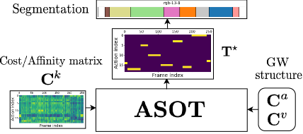
Figure 1: High-level overview of our action segmentation method, ASOT. Given a (noisy) cost/affinity matrix between video frames and actions, ASOT solves an optimal transport (OT) problem to yield temporally consistent segmentations.

Furthermore, successful approaches to unsupervised learning for image data based on joint representation learning and clustering [6, 45] have been adapted to the action segmentation task [23, 40], yielding state-of-the-art results. These methods use (regularized) optimal transport (OT) [9] to generate pseudo-labels for self-training, and jointly learn a video encoder and a set of action class embeddings. However, the OT formulation used in [23, 40] does not account for temporal consistency, which is inherent to the action segmentation task. In addition, the balanced assignment assumption is imposed, which yields pseudo-labels that are uniformly distributed among action classes. We argue this is unreasonable for action segmentation since datasets used [21, 2, 35] exhibit long-tailed class distributions [11].

Motivated by these observations, we propose Action Segmentation Optimal Transport (ASOT), a novel method for decoding a temporally consistent segmentation from a noisy affinity/matching cost matrix between video frames and action classes. ASOT involves solving a fused, unbalanced Gromov-Wasserstein (GW) optimal transport (OT) problem, which fuses visual information from the cost matrix with a structure-aware GW component that encourages temporal consistency. Unbalanced OT allows for only a subset of actions to be represented within a video. Fig. 1 illustrates the mechanics of ASOT.

Finally, we show that ASOT is generally applicable as a post-processing step for action segmentation pipelines. Unlike prior HMM-based approaches, ASOT handles order variations and repeated actions without knowing the action ordering. While we primarily evaluate ASOT in an unsupervised learning setting, we also show how ASOT is effective for post-processing of supervised methods. We thoroughly evaluate ASOT on the unsupervised action segmentation task, yielding state-of-the-art results. We provide an implementation of ASOT with training and evaluation code.

2 Related Work

Fully Supervised Action Segmentation.

Recent approaches for the action segmentation task in the fully-supervised setting have focused on developing appropriate model architectures. In particular, the temporal convolutional network (TCN) [24, 25] is widely used in the literature since it handles long-term dependencies through a temporal convolution layer. MS-TCN [13, 28] uses a multi-scale TCN so videos can be processed at a high temporal resolution. Recently, transformer style architectures are also being investigated [44, 5, 3], yielding promising results. Finally, some works propose additional segmentation refinement blocks on top of existing architectures [15, 1, 7]. Ad hoc smoothness losses are commonly included during training to encourage temporal consistency [13, 7, 44, 14]. We show how ASOT can be used as a post-processing step to further improve the performance of MS-TCN [28].

Unsupervised Action Segmentation.

In the unsupervised setting, learning by solving a proxy task is a common approach. Kukleva et al. [22] proposed CTE, which uses timestamp prediction as a proxy task. The output from intermediate network layers is used for the frame embeddings. UDE [36] and VTE [42] extend CTE with a discriminative embedding loss and visual reconstruction loss. These methods have two stages; representations are learned through the proxy task, and a clustering algorithm is subsequently used to recover actions. ASAL [26] alternate between representation learning and HMM parameter estimation using a generalized EM approach. Notably, TOT [23] and UFSA [40] are similar to our approach, performing joint representation learning and clustering using temporal OT.

However, TOT [23] suffers from three limitations: 1) a balanced assignment assumption is enforced on pseudo-labels, which we argue is unreasonable for long-tailed action class distributions encountered in action segmentation datasets [11], 2) temporal consistency is not addressed and 3) a single, fixed action ordering for all videos is assumed. UFSA [40] extends TOT [23] by relaxing 1) and 3) through two learned modules, an action transcript prediction module and a frame to transcript alignment module. In contrast, our method addresses all three limitations of TOT, handling order variations and repeated actions, by expanding the OT formulation, with no significant increase in learnable parameters or network architecture complexity from UFSA [40]. Furthermore, TOT [23] and UFSA [40] use a HMM approach to decode segmentations given a fixed (TOT) or estimated (UFSA) action ordering. In contrast, we can use ASOT for both pseudo-labelling and decoding.

We refer the reader to Ding et al. [11] for a comprehensive survey on the temporal action segmentation task.

Optimal Transport for Structured Prediction.

Optimal transport has been used for many alignment tasks in computer vision and machine learning, with too many applications to be listed here. See Khamis et al. [18] for a recent survey. Recent examples in computer vision include keypoint matching across image pairs [32, 29], point set registration [34] and training object detectors [10]. GW OT in particular, has been used for structured data, e.g., representation learning on graphs [43] and recently, aligning brains using fMRI scans[38]. For the first time, we use GW to exploit problem structure for a segmentation task. Our method has strong connections to post-processing methods for image segmentation problems, e.g., dense conditional random fields [20] and bilateral filtering [4], which is worth exploring in more detail in future work.

3 Optimal Transport on Structured Data

Our proposed method, ASOT, formulates the post-processing step of the temporal action segmentation task as an optimal transport problem. Specifically, we adopt a fused, unbalanced, Gromov-Wasserstein (FUGW OT) formulation. In this section, we will provide some background on optimal transport and specifically, the FUGW problem.

Preliminaries.

First, let $\langle\mathbf{A},\mathbf{B}\rangle\coloneqq\sum_{i,j}A_{ij},B_{ij}$ for $\mathbf{A},\mathbf{B}\in\mathbb{R}^{n\times m}$ and let $\mathbf{1}_{n}$ be a length $n$ vector of ones. Denote a dataset comprised of $B$ videos as $\mathcal{D}\coloneqq\{\mathcal{V}^{b}\}_{b=1}^{B}$. Each video is assumed to be comprised of $N$ frames, denoted $\mathcal{V}^{b}\coloneqq\{\mathcal{I}_{1}^{b},\dots,\mathcal{I}_{N}^{b}\}$. Furthermore, let $\mathbf{X}^{b}\coloneqq f_{\theta}(\mathcal{V}^{b})\in\mathbb{R}^{N\times D}$ denote frame-level embeddings for a single video, extracted using a deep network parameterized by $\theta$. Let (learnable) cluster centroids, which represent actions, be denoted $\mathbf{A}\coloneqq\left[\mathbf{a}_{1},\dots,\mathbf{a}_{K}\right]\in\mathbb{R}^{D\times K}$. Let $[n]\coloneqq\{1,\dots,n\}$ denote a discrete set with $n$ elements, and finally, let $\Delta_{K}\subset\mathbb{R}^{K}$ be the $K-1$ dimensional probability simplex and $\Delta_{K}^{N}\subset\mathbb{R}^{K\times N}$ denote the Cartesian product space comprised of $N$ such simplexes.

3.1 Kantorovich Optimal Transport

The classic optimal transport formulation is commonly known as the Kantorovich (KOT) formulation [37], and we focus on the discrete setting in this paper. Given histograms $\mathbf{p}\in\Delta_{n}$ and $\mathbf{q}\in\Delta_{m}$, and a ground cost $\mathbf{C}^{k}\in\mathbb{R}^{n\times m}_{+}$, the KOT problem solves for the minimum cost coupling $\mathbf{T}^{\star}$ between $\mathbf{p}$ and $\mathbf{q}$. Specifically, the problem is given by

$$\begin{array}[]{cc}\underset{\mathbf{T}\in\mathcal{T}_{\mathbf{p},\mathbf{q}}}{\text{minimize}}&\mathcal{F}_{\text{KOT}}(\mathbf{C}^{k},\mathbf{T})\coloneqq\langle\mathbf{C}^{k},\mathbf{T}\rangle,\end{array}$$ (1)

where $\mathcal{T}_{\mathbf{p},\mathbf{q}}\coloneqq\{\mathbf{T}\in\mathbb{R}_{+}^{n\times m}\mid\mathbf{T}\textbf{1}_{m}=\mathbf{p},\mathbf{T}^{\top}\textbf{1}_{n}=\mathbf{q}\}$ is commonly referred to as the transportation polytope. The coupling $\mathbf{T}$ can be interpreted as a soft assignment between elements in the support of $\mathbf{p}$ and $\mathbf{q}$, namely, two discrete sets denoted $[n]$ and $[m]$. In the context of action segmentation, coupling $\mathbf{T}\in\mathbb{R}^{N\times K}$ can be interpreted as an assignment between frames and actions.

3.2 Gromov-Wasserstein Optimal Transport

Gromov-Wasserstein (GW) optimal transport is an extension to the Kantorovich formulation, and is used for comparing histograms defined over incomparable spaces. Concretely, let $(\mathbf{C}^{v},\mathbf{p})\in\mathbb{R}^{n\times n}\times\Delta_{n}$ and $(\mathbf{C}^{a},\mathbf{q})\in\mathbb{R}^{m\times m}\times\Delta_{m}$ be two metric-measure pairs. The distance matrices, $\mathbf{C}^{v}$ (resp. $\mathbf{C}^{a})$ fully describe a metric defined over supports $[n]$ (resp. $[m]$). In the GW setting, there is no metric/cost defined between $[n]$ and $[m]$. The GW OT problem [30] replaces the KOT objective function in Eq. 1 with

$$\mathcal{F}_{\text{GW}}(\mathbf{C}^{v},\mathbf{C}^{a},\mathbf{T})\coloneqq\sum_{\begin{subarray}{c}i,k\in[n]\\ j,l\in[m]\end{subarray}}L(C_{ik}^{v},C_{jl}^{a})T_{ij}T_{kl},$$ (2)

where $L:\mathbb{R}\times\mathbb{R}\rightarrow\mathbb{R}$ is a cost function penalizing deviations between distance matrix elements. GW OT is commonly used to compare structured objects, e.g., graphs [30]. In our work, we use this GW formulation to encode structural priors over the transport map desirable for the video segmentation task (i.e., temporal consistency). This is achieved by setting $\mathbf{C}^{v}$ and $\mathbf{C}^{a}$ in a particular way, which will be described in detail in Sec. 4.2.

3.3 Fused GW Optimal Transport

The fused Gromov-Wasserstein (FGW) problem [41, 27, 38, 39] combines the KOT and GW OT formulations into a single optimization problem. The FGW formulation is useful when both a ground cost and a structural prior is available. FGW OT has been used previously in machine learning for graph classification and clustering [41] and aligning fMRI data [38]. Given parameter $\alpha\in[0,1]$, and letting $\mathbf{C}\coloneqq\{\mathbf{C}^{k},\mathbf{C}^{v},\mathbf{C}^{a}\}$, the FGW objective is given by

$$\mathcal{F}_{\text{FGW}}(\mathbf{C},\mathbf{T})\coloneqq\alpha\mathcal{F}_{\text{GW}}(\mathbf{C}^{v},\mathbf{C}^{a},\mathbf{T})+(1-\alpha)\mathcal{F}_{\text{KOT}}(\mathbf{C}^{k},\mathbf{T}).$$ (3)

For the temporal segmentation problem, the KOT component encodes visual similarity between the cluster/action representations and video frame embeddings. The GW component on the other hand, encodes desirable structural properties for resulting segmentations, i.e., temporal consistency. We will describe how parameters $\mathbf{C}$ are determined for action segmentation in Sec. 4.

3.4 Unbalanced Optimal Transport

Recently, there has been interest in unbalanced transport problems [38, 33, 8], where the constraint for $\mathbf{T}$ to lie in the transportation polytope $\mathcal{T}_{\mathbf{p},\mathbf{q}}$ (often referred to as the balanced assignment property) is relaxed. This can be achieved by replacing the marginal constraints on $\mathbf{T}$ with penalty terms in the objective function. Concretely, in this work, we will solve the optimization problem given by

$$\begin{array}[]{cc}\underset{\mathbf{T}\in\mathcal{T}_{\mathbf{p}}}{\text{minimize}}&\mathcal{F}_{\text{FGW}}(\mathbf{C},\mathbf{T})+\lambda\text{D}_{\text{KL}}(\mathbf{T}^{\top}\textbf{1}_{n}\|\mathbf{q}),\end{array}$$ (4)

where $\text{D}_{\text{KL}}(\mathbf{a}\|\mathbf{b})\coloneqq\sum_{i}a_{i}\log(a_{i}/b_{i})$ is the Kullback-Leibler divergence and $\mathcal{T}_{\mathbf{p}}\coloneqq\{\mathbf{T}\in\mathbb{R}_{+}^{n\times m}\mid\mathbf{T}\textbf{1}_{K}=\mathbf{p}\}$ is a partial polytope constraint over the row-sum marginal of $\mathbf{T}$. A penalty, weighted by $\lambda>0$, is applied between the column-sum marginal of $\mathbf{T}$ to $\mathbf{q}$. We will explain in Sec. 4.3 why the unbalanced formulation is important for the temporal segmentation task.

4 Action Segmentation Optimal Transport

In this section, we describe our proposed post-processing approach ASOT, for the action segmentation problem. First, we explain how to extract a temporally consistent segmentation from a (noisy) cost matrix between video frames and actions using optimal transport. These cost matrices are easily computed using learned video frame and action embeddings. Second, we introduce the fused, unbalanced Gromov-Wasserstein OT problem underlying ASOT. The importance of the unbalanced and GW components for the action segmentation problem will be described in detail. Finally, we discuss including entropy regularization, which allows us to develop a fast, iterative solution based on scaling algorithms [8, 33, 38, 30, 9].

4.1 Optimal Transport for Action Segmentation

Let $\mathbf{p}=\frac{1}{N}\textbf{1}_{N}$ and $\mathbf{q}=\frac{1}{K}\textbf{1}_{K}$ be histograms over the set of $N$ video frames and $K$ actions, denoted $[N]$ and $[K]$, respectively. An (optimal) coupling $\mathbf{T}^{\star}\in\mathbb{R}^{N\times K}$ between $[N]$ and $[K]$ can be interpreted as a (soft) assignment between video frames and actions. For frame $i$, we can predict the corresponding action using $j^{\star}=\mathop{\textrm{arg\,max}}_{j}\mathbf{T}_{ij}^{\star}$. Let $\mathbf{C}$ be the set of cost matrices for the KOT and GW sub-problems, which will be defined in Sec. 4.2. We solve the optimization problem in Eq. 4 for the coupling $\mathbf{T}^{\star}$.

4.2 Objective Function Formulation

Visual Information.

Given frame embeddings $\mathbf{X}$ and action embeddings $\mathbf{A}$, we can derive the matching cost matrix as $C^{k}_{ij}\coloneqq 1-\frac{\mathbf{x}_{i}^{\top}\mathbf{a}_{j}}{\|\mathbf{x}_{i}\|_{2}\|\mathbf{a}_{j}\|_{2}}$. This defines the KOT component of Eq. 4, and incorporates visual information from the videos through the frame encoder. However, the KOT component alone does not provide temporal consistency.

Structural Priors.

The GW component encourages temporal consistency over $\mathbf{T}$. Define the GW cost function as $L(a,b)\coloneqq ab$, radius parameter $r\in[0,1]$ and furthermore, let $\mathbf{C}^{v}\in\mathbb{R}^{N\times N}$ and $\mathbf{C}^{a}\in\mathbb{R}^{K\times K}$ be costs over video frames and action categories, respectively, given by

$$\mathbf{C}^{v}_{ik}\coloneqq\begin{cases}1/r&1\leq|i-k|\leq Nr\\ 0&\text{o/w}\end{cases},\,\,\mathbf{C}^{a}_{jl}\coloneqq\begin{cases}0&j=l\\ 1&\text{o/w}\end{cases}.$$ (5)

This GW formulation penalizes couplings with low temporal consistency. Specifically, assigning temporally adjacent frames (within a radius of $Nr$ frames) to different actions incurs a cost in the GW objective in Eq. 2. To see this, let $T_{ij}$ and $T_{kl}$ represent two assignment probabilities with $|i-k|\leq Nr$, $i\neq k$ (adjacent) and $j\neq l$ (different actions). A cost of $T_{ij}T_{kl}$ is incurred in Eq. 2, since $L(C_{ik}^{\mathbf{p}},C_{jl}^{\mathbf{q}})=1$. On the other hand, action changes outside of a temporal interval ($|i-k|>Nr$) incur no cost nor does mapping adjacent frames to the same action ($j=l$). Fig. 2(b) and 2(c) illustrates the effect of the GW component.

Finally, note that we can compute Eq. 2 efficiently as $\mathcal{F}_{\text{GW}}(\mathbf{C}^{v},\mathbf{C}^{a},\mathbf{T})=\langle\mathbf{C}^{v}\mathbf{T}\mathbf{C}^{a},\mathbf{T}\rangle$ since the loss $L(a,b)=ab$ can be factorized, following Peyré et al. [30].

4.3 Importance of Unbalanced Transport

For the temporal action segmentation task, a balanced assignment necessitates that each video frame is assigned to an action and furthermore, that each action is represented equally across the frames of a video. While assigning each video frame to an action is required for the segmentation task, not every action may occur within a video. The partial polytope constraint in Sec. 3.4, i.e., $\mathbf{T}\in\mathcal{T}_{\mathbf{p}}$, ensures that every frame is assigned to an action. However, we do not force every action to be evenly represented over video frames. Instead, we regularize the distribution of actions observed within a video towards uniformity using a KL-divergence penalty weighted by $\lambda>0$. Setting lower values for $\lambda$ allows ASOT to find a segmentation that faithfully replicate the learned embeddings, whereas a high $\lambda$ emphasises that the segmentation is balanced across actions. Fig. 2(b) and 2(d) illustrates balanced and unbalanced OT.

4.4 Fast Numerical Solver for ASOT

We add an entropy regularization term $-\epsilon H(\mathbf{T})$, where $H(\mathbf{T})\coloneqq-\sum_{i,j}T_{ij}\log T_{ij}$ and $\epsilon>0$, into the objective function in Eq. 4. We can solve the FUGW problem using projected mirror descent similar to [30], which is amenable for computation on GPUs. Our solver typically converges within 25 iterations, with each iteration having time complexity $O(NK)$ after exploiting the sparsity structure of $\mathbf{C}^{v}$ and $\mathbf{C}^{a}$. We provide more details and psuedocode in the appendix. The largest video we encountered (in the 50Salads [35] dataset) had $N=16k$ frames and $K=19$ action classes and takes 26.1ms on an Nvidia RTX 4090 GPU.

(a) Affinity matrix $1-\mathbf{C}^{k}$.

(b) ASOT solution.

(c) ASOT w/no GW ($\alpha=0$).

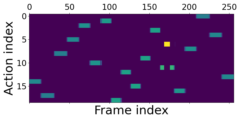
(d) ASOT w/out unbalanced OT.

Figure 2: A raw frame/action affinity matrix in a) is decoded using ASOT into a temporally consistent segmentation in b). Removing GW from b) destroys temporal consistency, shown in c). Forcing a balanced assignment to actions in b) yields temporally consistent, but unintuitive results, shown in d).

5 Unsupervised Learning Pipeline

In this section, we will describe our simple representation learning pipeline for unsupervised action segmentation. Core to our method is a self-training approach; we use ASOT described in Sec. 4 to generate pseudo-labels, which are then used to train a video frame encoder. Fig. 3 illustrates the representation learning pipeline.

Learning Problem.

Our unsupervised problem involves learning the parameters $\theta$ of a video frame encoder by minimizing the cross-entropy (CE) loss between frame/action embedding similarities and (soft) pseudo-labels computed by ASOT. Concretely, let $\mathbf{P}^{b}\in\Delta_{K}^{N}$ be normalized similarities for batch element $b$, defined element-wise as

$$P^{b}_{ij}\coloneqq\frac{\exp(\mathbf{X}^{b}\mathbf{A}^{\top}/\tau)_{ij}}{\sum_{l}\exp(\mathbf{X}^{b}\mathbf{A}^{\top}/\tau)_{il}},$$ (6)

where $\tau>0$ is a temperature scaling parameter. Next, soft-pseudo labels $\mathbf{T}^{b}\in\mathbb{R}^{K\times N}$ are derived from the solution to the optimization problem in Eq. 4, parameterized using a KOT cost matrix given by $\hat{\mathbf{C}}^{k}=\mathbf{C}^{k}+\rho\mathbf{R}$ where $\rho\geq 0$.

Here $\mathbf{R}$ is a temporal prior, introduced in [23], defined element-wise as $R_{ij}=\left|i/N-j/K\right|$. $\mathbf{R}$ regularizes the coupling towards a banded diagonal and encourages a canonical ordering of actions across videos. We find setting $\rho>0$ encourages correspondences between adjacent frames across videos, improving clustering performance.

Our representation learning loss is given by

$$\mathcal{L}_{\text{train}}(\theta)=-\frac{1}{B}\sum_{b=1}^{B}\sum_{i=1}^{N}\sum_{j=1}^{k}T^{b}_{ij}\log P^{b}_{ij}.$$ (7)

Same as in prior works [6, 23], we apply a stop-gradient through pseudo-labels $\mathbf{T}^{b}$. The learnable parameters include the feature extractor $\theta$ as well as action embeddings $\mathbf{A}$. We parameterize $f_{\theta}$ as a multi-layer perceptron (MLP) applied per frame, consistent with prior works [22, 26, 23].

Figure 3: The unsupervised training pipeline. Orange are learnable parameters, and arrows indicate computation/gradient flow.

6 Experimental Setup

Implementation Details.

The encoder MLP has one hidden layer and we use the Adam optimizer [19] with a learning rate of $10^{-3}$ and weight decay of $10^{-4}$. We use $k$-means to initialize the action embeddings. During training, we sample 256 frames randomly from uniformly spaced bins within each video, similar to [23]. A full description of hyperparameter settings is provided in the appendix. We set $K$ to be equal to the ground truth number of actions per activity category/dataset, consistent with prior works [22, 26, 23, 40].

Datasets.

We briefly describe the four video datasets we use to evaluate our method. All unsupervised methods are trained and evaluated on the same set of videos. While videos are subsampled during training for our method, we use full videos during testing. For Breakfast and YouTube Instructions, we train and evaluate our method per activity category and aggregate results.

• The Breakfast (BF) dataset [21] consists of approx. 1,700 videos, where each video captures a subject preparing a breakfast item. The dataset is split across activity categories, where each activity category corresponds to a particular item (e.g., scrambled egg, juice). Within each video, multiple actions are observed (e.g., crack egg, pour flour). Breakfast contains 10 activity categories with 48 actions across all activities, and videos range from a few seconds to several minutes. We use pre-computed Fisher vector features from images, consistent with prior works [22, 26, 23].

• The YouTube Instructions (YTI) dataset [2] includes 150 instructional videos belonging to 5 activity categories. The average video lasts approx. 2 minutes, and this dataset also has a large number of background frames. We use pre-computed image features provided by [2], consistent with prior works [22, 26, 23].

• The 50 Salads (FS) dataset [35] contains 50 videos of actors performing a cooking activity, totalling 4.5 hours in length. Consistent with prior works, we report results at two action granularity levels, i.e., Mid with 19 action classes and Eval with 12 action classes. The Eval level aggregates some actions in the Mid level into a single action. We use pre-computed features which were used in prior works [22, 26, 23].

• The Desktop Assembly (DA) dataset [23] includes 76 videos of actors performing an assembly activity. The activity comprises 22 actions conducted in a fixed order. Each video is approx. 1.5 minutes long, and we use the pre-computed features provided by [23].

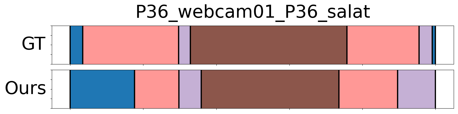
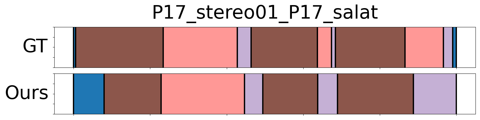
(a) Example videos from the “salat” activity class within the Breakfast dataset, exhibiting order variations and repeated actions. Both cases are handled by ASOT. Actions classes shown are cut fruit, peel fruit, fruit to bowl, background.

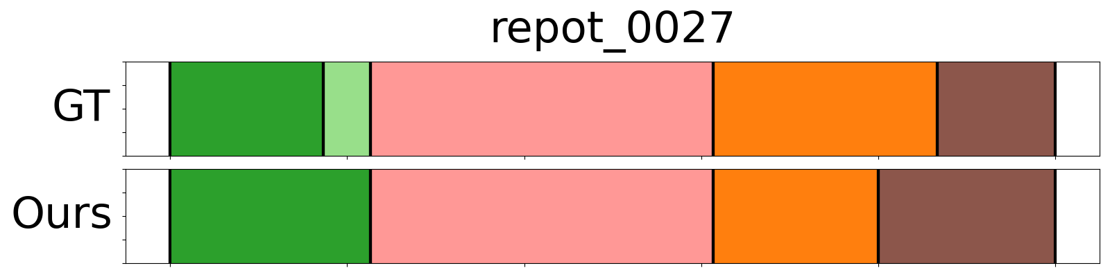
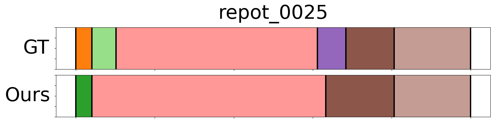
(b) Example videos from YTI (“repot” category). Actions classes shown are tap pot, take plant, loosen root, put soil, add top, water plant, place plant.

Figure 4: Example action segmentations for videos in the same activity category with differing action orderings. Different colors correspond to different actions. Videos of complex, multi-stage activities can be exhibit markedly different action orderings.

Evaluation Metrics.

We follow an evaluation protocol consistent with prior works on the unsupervised segmentation task [22, 26, 23, 42, 36], which we will now describe. Since no ground truth action labels are used during training, we perform Hungarian matching to match learned action clusters to ground truth actions using frame labels and predictions. We evaluate methods under two settings, where the Hungarian matching is performed per video (Unsup. per) and across the full dataset (Unsup. full). Matching per video does not require clusters to match to the same ground truth action across videos and yields more favorable results.

We comprehensively evaluate all methods using mean-over-frames (MoF), F1-score and mean intersection-over-union (mIoU). MoF measures the percentage of correct per-frame predictions and is susceptible to class imbalance issues in a dataset. The F1-score is defined on a per-segment basis, where a true positive is defined as having over 50% of the frames in a ground truth segment predicted correctly. The F1-score is complementary to MoF since large segments (from dominant classes) are treated a single segment. Finally, mIoU computes the IoU averaged over all classes, and is again complementary to both MoF and F1 because because it explicitly handles class imbalance.

Comparison Methods.

We compare our approach against multiple prior works on unsupervised action segmentation [22, 26, 23, 42, 36, 40]. Common to all of these prior approaches is that post-processing involves solving an inference problem in some underlying hidden Markov model (HMM). The states in the HMM correspond to learned action clusters, and observation likelihoods correspond to frame/cluster similarities. A core assumption around the HMM is that the action ordering is known for all videos, which informs the structure of the transition matrix.

All approaches apart from [40] assume a fixed action ordering for all videos a priori, whereas [40] estimates the action ordering per video using an action transcript prediction module. However, our unsupervised learning pipeline uses ASOT for post-processing and does not need these restrictive assumptions or additional learned modules.

We also add a comparison to unsupervised methods which perform Hungarian matching and evaluate per video (Unsup. per) [31, 12]. For our method, we can use the clusters and frame features learned over the full dataset but evaluate metrics using Hungarian matching per video. TW-FINCH (TWF) [31] applies clusters time-weighted frame features within a single video and uses cluster assignments for segmentation. ABD [12] uses a change detection approach applied over image similarities computed from adjacent video frames. As discussed previously, per video matching tends to yield (much) more favorable results.

		Breakfast	YouTube Instr.	50 Salads (Mid)	50 Salads (Eval)	Desktop Ass.
		MoF / F1 / mIoU	MoF / F1 / mIoU	MoF / F1 / mIoU	MoF / F1 / mIoU	MoF / F1 / mIoU
Per Video	TWF [31]	62.7 / 49.8 / 42.3	56.7 / 48.2 /     -	66.8 / 56.4 / 48.7	71.7 /     -     /     -	73.3 / 67.7 / 57.7
	ABD [12]	64.0 / 52.3 /     -	67.2 / 49.2 /     -	71.8 /     -     /     -	71.2 /     -     /     -	-     /     -     /     -
	ASOT (Ours)	63.3 / 53.5 / 35.9	71.2 / 63.3 / 47.8	64.3 / 51.1 / 33.4	64.5 / 58.9 / 33.0	73.4 / 68.0 / 47.6
Full	CTE∗ [22]	41.8 / 26.4 /     -	39.0 / 28.3 /     -	30.2 /     -     /     -	35.5 /     -     /     -	47.6 / 44.9 /     -
	CTE† [22]	47.2 / 27.0 / 14.9	35.9 / 28.0 /   9.9	30.1 / 25.5 / 17.9	35.0 / 35.5 / 21.6	-     /     -     /     -
	VTE [42]	48.1 /     -     /     -	-     / 29.9 /     -	24.2 /     -     /    -	30.6 /     -     /     -	-     /     -     /     -
	UDE [36]	47.4 / 31.9 /     -	43.8 / 29.6 /     -	-     /     -     /     -	42.2 / 34.4 /     -	-     /     -     /     -
	ASAL [26]	52.5 / 37.9 /     -	44.9 / 32.1 /     -	34.4 /     -     /     -	39.2 /     -     /     -	-     /     -     /     -
	TOT [23]	47.5 / 31.0 /     -	40.6 / 30.0 /     -	31.8 /     -     /     -	47.4 / 42.8 /     -	56.3 / 51.7 /     -
	TOT+ [23]	39.0 / 30.3 /     -	45.3 / 32.9 /     -	34.3 /     -     /     -	44.5 / 48.2 /     -	58.1 / 53.4 /     -
	UFSA (M) [40]	-     /     -     /     -	43.2 / 30.5 /     -	-     /     -     /     -	47.8 / 34.8 /     -	-     /     -     /     -
	UFSA (T) [40]	52.1 / 38.0 /     -	49.6 / 32.4 /     -	36.7 / 30.4 /     -	55.8 / 50.3 /     -	65.4 / 63.0 /     -
	ASOT (Ours)	56.1 / 38.3 / 18.6	52.9 / 35.1 / 24.7	46.2 / 37.4 / 24.9	59.3 / 53.6 / 30.1	70.4 / 68.0 / 45.9

Table 1: Summary of experimental results. For all evaluation metrics, higher is better and bold (respectively, underline) indicates the best (respectively second best) performing methods. A “-” indicates that a metric was not reported in the original paper. Note that “Full” and “Per Video” relate to the evaluation metrics being computed by applying Hungarian matching on a whole dataset and per video basis, respectively. For CTE [22], $\ast$ and $\dagger$ indicate results reported and reproduced using model checkpoints provided by the authors, respectively. Results were generated using one run, consistent with prior works, however we provide results for 5 runs for FS and DA in the appendix.

	Breakfast	YouTube Instr.	50 Salads (Mid)	50 Salads (Eval)	Desktop Ass.
	MoF / F1 / mIoU	MoF / F1 / mIoU	MoF / F1 / mIoU	MoF / F1 / mIoU	MoF / F1 / mIoU
Base	56.1 / 38.3 / 18.6	52.9 / 35.1 / 24.7	46.2 / 37.4 / 24.9	59.3 / 53.6 / 30.1	70.4 / 68.0 / 45.9
No $k$-means	57.7 / 36.0 / 17.1	49.5 / 34.1 / 21.3	42.1 / 34.5 / 22.1	55.2 / 52.7 / 28.2	56.8 / 61.7 / 35.6
No temp. prior	48.5 / 24.9 / 16.3	46.9 / 26.2 / 14.6	43.1 / 36.5 / 21.9	59.7 / 54.7 / 26.3	31.4 / 18.7 / 10.6
Balanced OT	29.7 / 29.3 / 17.8	39.4 / 31.4 / 14.6	39.7 / 39.8 / 25.3	35.7 / 41.8 / 24.9	56.5 / 72.7 / 37.8
No GW (train)	34.4 / 25.9 / 14.4	41.1 / 24.9 / 11.7	29.0 / 22.6 / 14.3	35.1 / 38.6 / 22.5	49.5 / 49.4 / 30.4
No GW (train & test)	32.6 / 21.3 / 10.4	38.0 / 21.8 / 11.9	17.3 /    4.2 /    8.9	25.8 / 21.3 / 14.8	45.4 / 42.0 / 26.5

Table 2: Ablation study results for the Unsup (full) setting. Effects are not additive. For all evaluation metrics, higher is better.

7 Results

7.1 State-of-the-Art Comparison

Our experimental results are presented in Tab. 1. For the Unsup. (full) setting, our method consistently outperforms all relevant prior works across all evaluation metrics. For the Breakfast dataset, our method yields comparable results to ASAL [26] and the recent joint representation learning and clustering approach UFSA [40], where UFSA (T) in Tab. 1 refers to the authors’ full model with a transformer frame encoder. However, we show major improvements over UFSA (T) for the FS (Mid) and DA datasets.

We note that our method uses a simple MLP frame encoder, whereas UFSA uses a more complex transformer encoder, on top of multiple additional learned modules. For a fairer comparison, we also present results for UFSA with a comparable MLP encoder, displayed as UFSA (M) in Tab. 1. Compared to UFSA (M), we show significant improvements for YTI and FS (Eval). Similar to UFSA, we believe our method’s ability to handle out-of-order alignments during segmentation contributes to the improved performance. Fig. 4 contains qualitative examples where actions are seen in different orders across videos within a dataset.

For the per video evaluation protocol, our method outperforms TWF [31] and ABD [12] on the BF and YTI datasts for MoF and F1, however for BF it performs poorly on mIoU. We believe this is because our method is more successfully finding segmentation boundaries for large classes, at the cost of failing to identify shorter, more underrepresented actions. In addition, our method appears to underperform on FS (Mid and Eval) and yield comparable results for DA. We emphasize that the results were optimized for the Unsup. (full) setting, where actions should be identified correctly across videos. An interesting avenue for future work is to investigate how to estimate action clusters using frame features from a single video for our method.

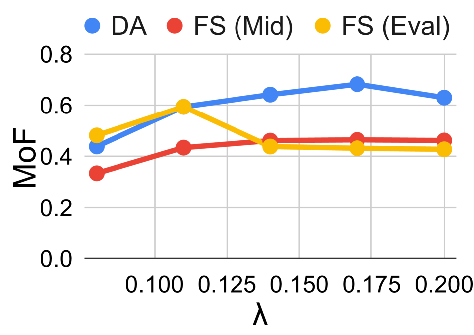
(a) Balanc. assign. weight $\lambda$

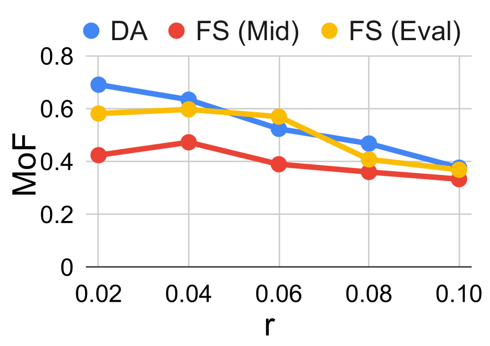
(b) GW radius $r$

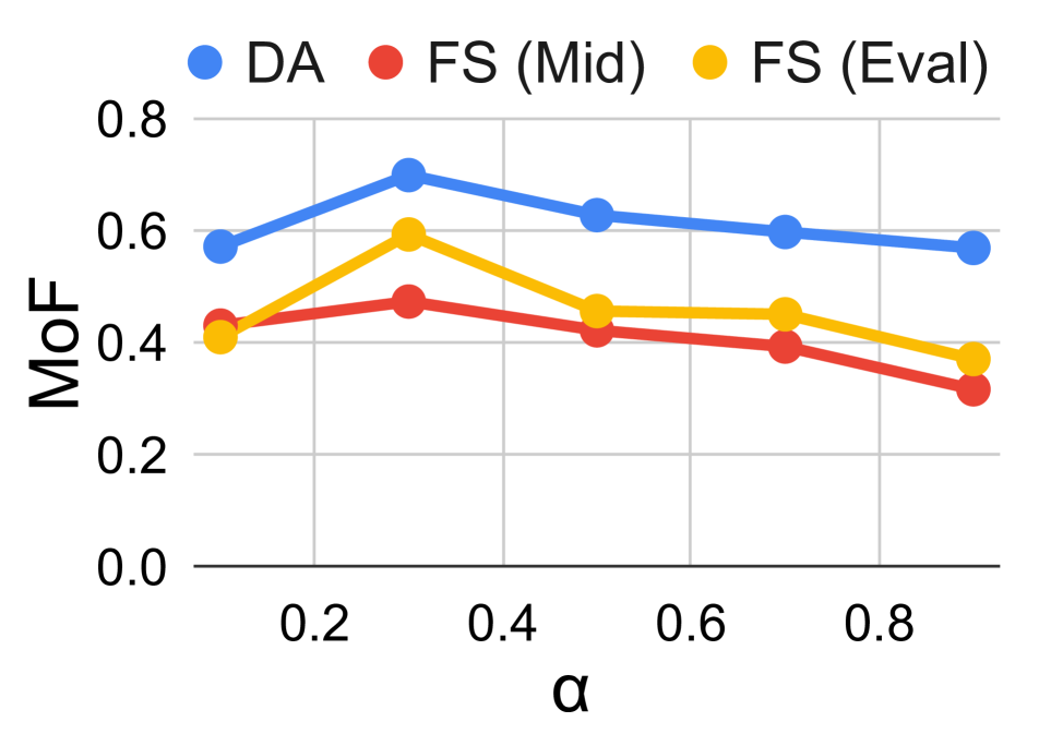
(c) GW weight $\alpha$

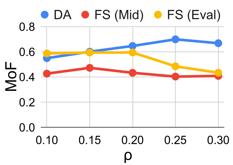
(d) Global temporal prior $\rho$

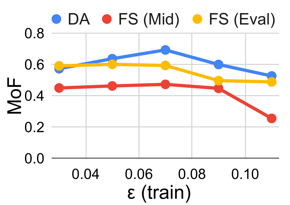
(e) Entropy reg. $\epsilon_{\text{train}}$

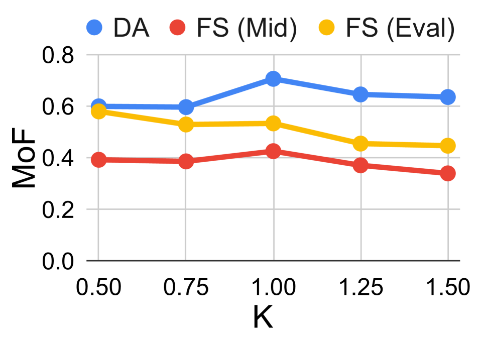
(f) Ratio of learned/true actions

Figure 5: Sensitivity analysis on FUGW OT hyperparameters.

7.2 Ablation Study

In this section, we analyze the effects of various choices in our learning pipeline and present the results in Table 2.

Temporal prior and $k$-means.

First, we ablate the effect of initialization of action clusters by switching $k$-means to random sampling (No $k$-means). We find that overall, using $k$-means is beneficial because the clusters are initialized to be more evenly represented within videos, yielding higher quality pseudo-labels at the start of training. Second, we remove the temporal prior (No temp. prior) described in Sec. 5. The prior appears to yield a positive effect overall.

Effect of (un)balanced assignment.

For ASOT, we first analyze the effect of forcing a balanced assignment to actions (Balanced OT), ignoring the unbalanced OT formulation described in Sec. 4.3. For the BF, YTI and FS datasets, we observed that dominant classes are common in the ground truth annotations, and forcing a balanced assignment to actions severely degrades performance overall. However for DA, enforcing a balanced assignment actually slightly improves performance. This is because the ground truth actions are (relatively) evenly represented across the DA dataset. Compare Figures 6(b) and 4 to Figure 6(a) to see class balance discrepancies across datasets.

Effect of GW structural prior.

Finally, we remove the GW problem described in Sec. 3.2 at training time only (No GW (train)), as well as at both training and test time (No GW (train & test)). We observe that removing the temporal consistency of the pseudo-labels alone is enough to compromise the performance of our method. As expected, also removing the temporal consistency of the test time segmentations further reduces performance.

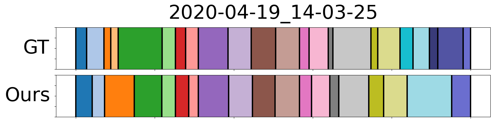
(a) Desktop Assembly

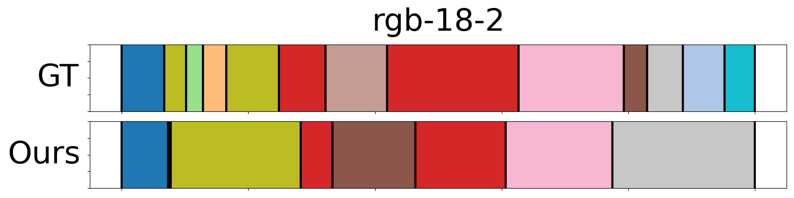
(b) 50 Salads (Eval)

Figure 6: Example segmentations from DA and FS (Eval). Note the dominant red class in FS, whereas DA is (roughly) balanced.

7.3 Sensitivity Analysis

In addition to the ablation studies, we performed a sensitivity analysis on the hyperparameters of our action segmentation OT method during training. These hyperparameters strongly influence the behavior of the pseudo-labels and resultant learned representations. We illustrate the results in Fig. 5 and perform this analysis using the desktop assembly (DA) and 50 Salads (FS) datasets at both the Eval and Mid granularity, using MoF as the metric.

Effect of $\lambda$, $r$ and $\alpha$.

As discussed in Sec. 7.2, a (more) balanced assignment benefits datasets such as DA and FS (Mid) with a large number of action classes. Unsurprisingly, MoF improves for DA and FS (Mid) for increasing $\lambda$, whereas FS (Eval), which has more dominant action classes, has an optimal point around $\lambda=0.11$. Furthermore, the GW radius $r$ is positively correlated to the resulting segment length. We can see that a small value of $r=0.02$ is enough for temporal consistency in FS (Mid and Eval) and DA, yielding the best MoF. Finally, MoF is relatively insensitive to the GW structure weight $\alpha$, except at the extremes. We find a value of $\alpha\in[0.2,0.5]$ to work well across all evaluated datasets.

Effect of $\rho$, $\epsilon_{\text{train}}$ and $K$.

Finally, we observe that higher values for the global temporal prior weight $\rho$ benefits DA. We believe this is because a (banded) diagonal coupling is a reasonable solution for datasets such as DA with relatively balanced action classes and identical action orderings across videos. However, FS (Eval and Mid) seem to benefit from removing the global prior altogether. The pseudo-labels at initialization appear to be high quality, and do not need additional guidance from the global structure.

Furthermore, we observe that the optimal value for entropy regularization for the OT problem, denoted $\epsilon_{\text{train}}$, should be set between 0.06 and 0.08. Low values for $\epsilon_{\text{train}}$ may result in numerical instability arising from the solver, while high values may result in incoherent segmentations. Finally, for datasets large number of classes (DA and FS Mid), setting number the of clusters $K$ to be equal to true number of actions $K_{\text{gt}}$ appears to be optimal. For FS (Eval) where dominant classes as present, performance actually improves by setting fewer clusters.

7.4 Post-Processing for Supervised Methods

We show the generality of ASOT as a post-processing method by applying it to the outputs of the supervised method MS-TCN++ [28] for the 50 Salads dataset. We use the recommended multi-scale configuration (MS) with three refinement layers as well as without refinement layers, i.e., single-scale (SS). [28] observed that the primary function of the refinement layers is to improve the temporal consistency of the predictions. Our results verify this finding, since SS with ASOT yields comparable performance with MS. Furthermore, applying ASOT to MS yields significant further improvements. See the appendix for hyperparameter settings and more details on this experiment.

	Accuracy	ED	F1@10	F1@25	F1@50
MS	83.5	72.6	80.1	77.2	69.4
SS	76.0	36.3	44.8	42.3	34.9
MS + ASOT	83.6	77.6	84.4	83.1	74.9
SS + ASOT	78.3	72.5	80.3	78.5	69.9

Table 3: ED and F1@$N$ refers to the segmental edit distance and F1 score at overlapping threshold of $N\%$, respectively. Acc. is the MoF accuracy. Higher is better for all metrics.

8 Discussion and Conclusion

In this paper we present a novel method for the unsupervised action segmentation task on long, untrimmed videos. Our post-processing approach ASOT, yields temporally consistent segmentations without prior knowledge of the action ordering, required by previous approaches. Furthermore, we show that in the unsupervised setting, ASOT produces pseudo-labels suitable for self-training. Future work will investigate the semi and fully-supervised action segmentation settings, which will require backpropagating through our ASOT problem. Finally, developing methods for unsupervised learning over all activity categories for challenging datasets such as Breakfast is an important direction for future work, and will require a more sophisticated learning pipeline than the one proposed in Sec. 5.

Acknowledgements.

This work was supported by an Australian Research Council (ARC) Linkage grant (project number LP210200931). Ming Xu thanks Akshay Asthana and Liang Zheng for helpful discussions about this work.

Appendix A Pseudo-code for ASOT

In Alg. 1, we present pseudo-code around the numerical solver for our action segmentation optimal transport (ASOT) algorithm. Our approach is based on projected mirror descent, similar to Peyre et al. [30]. We initialize the coupling $\mathbf{T}$ element-wise as $\mathbf{T}_{ij}=1/(NK)$. Each iteration then involves two steps, given by

1. Update step (Lines 6–16): The first-order update step is computed as a mirror descent step under the KL-divergence. The update step at iteration $t$ is given by $\hat{\mathbf{T}}^{t+1}=\mathbf{T}^{t}\odot\exp(-\phi\nabla_{\mathbf{T}}^{t}\mathcal{F}_{\text{ASOT}}(\mathbf{C},\mathbf{T}^{t}))$, where $\phi>0$ is a step size and

   $$\mathcal{F}_{\text{ASOT}}(\mathbf{C},\mathbf{T},\epsilon)\coloneqq \mathcal{F}_{\text{FGW}}(\mathbf{C},\mathbf{T})+$$

   $$\lambda\text{D}_{\text{KL}}(\mathbf{T}^{\top}\mathbf{1}_{n}\|\mathbf{q})-\epsilon H(\mathbf{T}).$$ (8)

2. Projection step (Lines 10–15): The projection step involves ensuring the polytope constraints are satisfied. This involves simply rescaling the rows of $\mathbf{T}$, to satisfy the frame-wise marginal constraint, i.e., $T^{t+1}_{ij}=p_{i}\hat{T}_{ij}^{t+1}/(\hat{\mathbf{T}}^{t+1}\mathbf{1}_{K})_{i}$.

Algorithm 1 Action Segmentation Optimal Transport

1:Video frame to action class affinity matrix $\mathbf{C}^{k}\in\mathbb{R}^{N\times K}$, derived from a video encoder and hyperparameters $\alpha\in[0,1]$, $r\in[0,1]$, $\lambda\geq 0$, $\epsilon>0$, $\phi>0$, $n_{\text{iter}}>0$.

2:Soft assignment probabilities $\mathbf{T}^{\star}\in\mathbb{R}^{N\times K}_{+}$.

3:function ASOT($\mathbf{C}^{k}$, $\alpha$, $r$, $\lambda$, $\epsilon$, $\phi$, $n_{\text{iter}}$)

4:     $\mathbf{p}\leftarrow\frac{1}{N}\mathbf{1}_{N}$ $\triangleright$ Frame marginals

5:     $\mathbf{q}\leftarrow\frac{1}{K}\mathbf{1}_{K}$ $\triangleright$ Balanced action marginals

6:     Construct $\mathbf{C}^{v}$, $\mathbf{C}^{a}$ using (5).

7:     $\mathbf{C}=\{\mathbf{C}^{k},\mathbf{C}^{v},\mathbf{C}^{a}\}$

8:     $\mathbf{T}^{0}\leftarrow\mathbf{p}\otimes\mathbf{q}$ $\triangleright$ $\otimes$ denotes the outer product

9:     for $t\leftarrow 0$ to $n_{\text{iter}}-1$ do

10:         $\hat{\mathbf{T}}^{t+1}=\mathbf{T}^{t}\odot\exp(-\phi\nabla_{\mathbf{T}}\mathcal{F}_{\text{ASOT}}(\mathbf{C},\mathbf{T}^{t}))$

11:         $T^{t+1}_{ij}=p_{i}\hat{T}_{ij}^{t+1}/(\hat{\mathbf{T}}^{t+1}\mathbf{1}_{K})_{i}\quad\forall i,j$

12:     end for

13:     return $\mathbf{T}^{n_{\text{iter}}}$

14:end function

We provide a full reference implementation for ASOT and training code at https://github.com/mingu6/action_seg_ot.

Appendix B Additional Details for Unsupervised Experiment

For both the training (pseudo-labelling) and inference phases, we use 25 iterations for projected mirror descent (see Sec. A). We use the same Gromov-Wasserstein (GW) radius parameter $r$ across training and inference, which is set at 0.04 for all datasets except for desktop assembly, which is set at 0.02. We observed that desktop assembly has smaller ground truth segments relative to video length, benefiting a lower value for $r$.

ASOT pseudo-labelling.

The ASOT hyperparameters used to generate pseudo-labels during the training phase of our unsupervised action segmentation pipeline are described as follows. The GW structure weight $\alpha$ is set to 0.3 for all datasets except for Breakfast where $\alpha=0.4$ and furthermore, entropy regularization weight $\epsilon=0.07$ for all datasets. Table 4 presents the remaining hyperparameters.

ASOT inference.

The hyperparameters used to generate segmentations from embeddings learned from our unsupervised learning pipeline are described as follows. First, we set the unbalanced weight $\lambda$ to a low value (0.01) for all datasets. At inference, ASOT will segment according to the underlying learned embeddings, and will not encourage a more balanced assignment to action classes. Second, we set $\alpha=0.6$ for all datasets except for Breakfast where $\alpha=0.7$, because a higher value for $\alpha$ results in stronger temporal consistency due to heavier weighting of the GW structure objective. Finally, we set $\epsilon=0.04$, since lower levels of entropy regularization yields sharper segmentations.

Representation learning.

We set the learning rate at $10^{-3}$ and weight decay to $10^{-4}$ for all datasets. We sample a batch of 2 videos, where for each video, we sample 256 frames randomly by partitioning each video into 256 uniform intervals and sampling a single frame from each interval. Our MLP architecture has a single hidden layer with ReLU activations. The hidden layer size is 128 for all datasets, with an output feature dimension of 40, with the exception of YouTube Instructions (YTI), which have sizes 32 and 32, respectively. Output features are $l_{2}$-normalized before applying ASOT. The smaller model size from YTI arises from the significantly higher dimensional input features compared to the remaining datasets.

	BF	YTI	FS (M)	FS (E)	DA
Unbalanced ($\lambda$)	0.1	0.12	0.15	0.11	0.16
Global prior ($\rho$)	0.2	0.15	0.15	0.15	0.25
Num. epochs	15	10	30	30	30

Table 4: Hyperparameter settings for ASOT used to generate pseudo-labels in the training phase of our unsupervised action segmentation pipeline. FS (M) and FS (E) represent the 50 Salads Mid and Eval splits, respectively.

Appendix C Experimental Setup (Supervised)

For the supervised example, the MS-TCN [28] architecture outputs logits $\mathbf{L}\in\mathbb{R}^{N\times K}$ directly instead of video frame and action embeddings. We can transform these logits into a cost matrix $\mathbf{C}^{k}$ using

$$C^{k}_{ij}=2\left(1-\frac{L_{ij}-L_{\text{min}}}{L_{\text{max}}-L_{\text{min}}}\right),$$ (9)

where $L_{\text{max}}\coloneqq\max_{i,j}L_{ij}$ and $L_{\text{min}}\coloneqq\min_{i,j}L_{ij}$. This is a simple method for converting the logits which model a frame/action affinity into a cost matrix with elements scaled between $[0,2]$.

We then apply ASOT to the cost matrix derived per video with hyperparameters $\lambda=0.05$, $\alpha=0.4$, $\epsilon=0.06$ and $r=0.01$. We evaluate our method using 5-fold cross validation, similar to [28].

Appendix D Additional Sensitivity Analysis

In addition to the sensitivity analysis under the MoF metric presented in Fig. 5, we present additional results for F1-score and mIoU in Fig. 7 and 8, respectively. The results follow very similar trends to MoF, however it is notable in Fig. 8(a) that mIoU performance collapses to almost 0 for $\lambda=0$, whereas MoF does not (see Fig. 5(a)). This is especially notable for the FS (Eval) dataset. This discrepancy between MoF and mIoU suggests the presence of unbalanced classes within the datasets, especially FS (Eval).

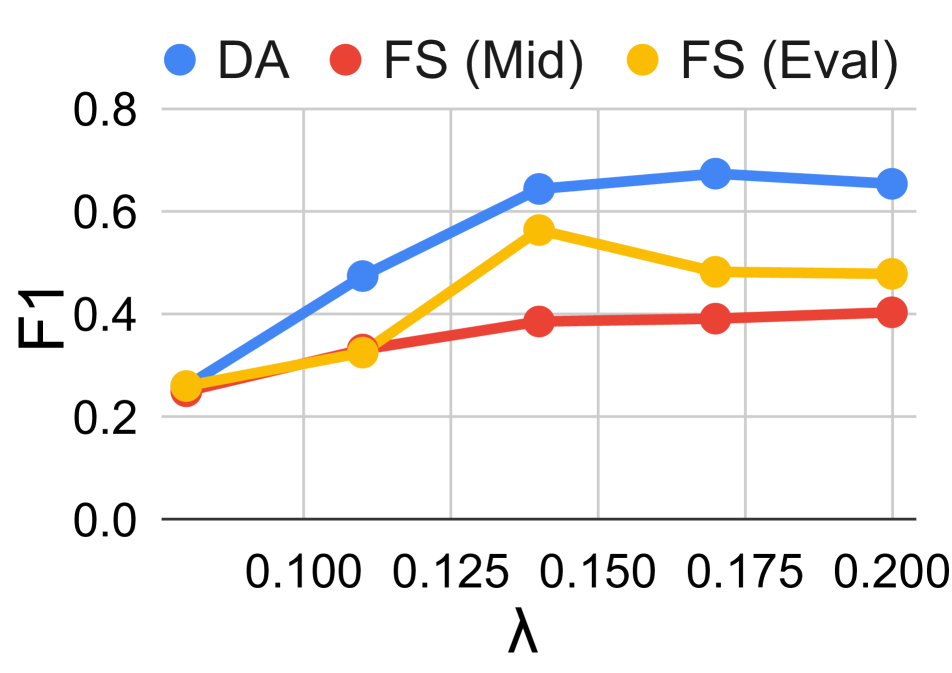
(a) Balanc. assign. weight $\lambda$

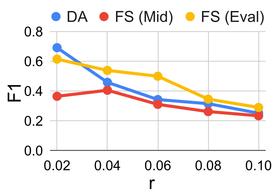
(b) GW radius $r$

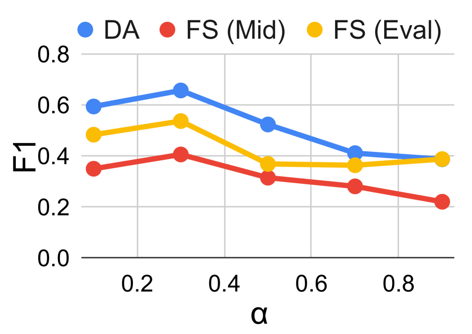
(c) GW weight $\alpha$

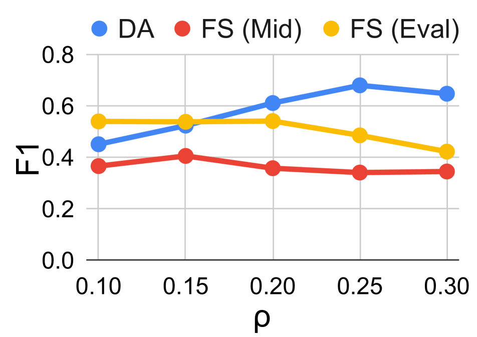
(d) Global temporal prior $\rho$

(e) Entropy reg. $\epsilon_{\text{train}}$

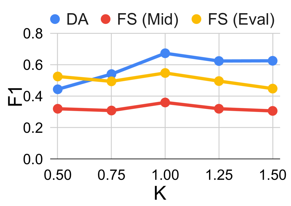
(f) Ratio of learned/true actions

Figure 7: Sensitivity analysis reporting F1-score on ASOT hyperparameters.

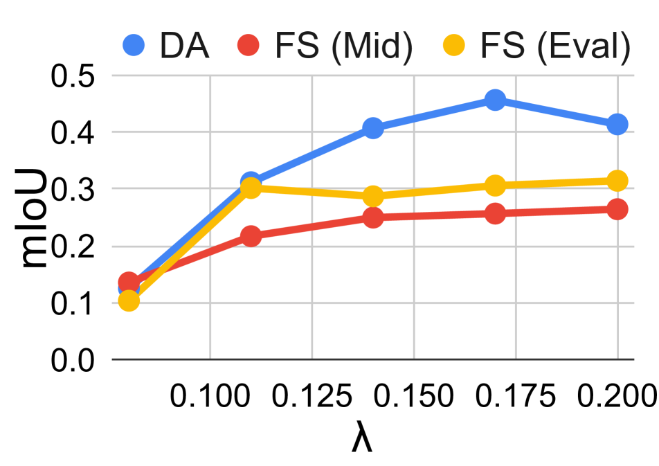
(a) Balanc. assign. weight $\lambda$

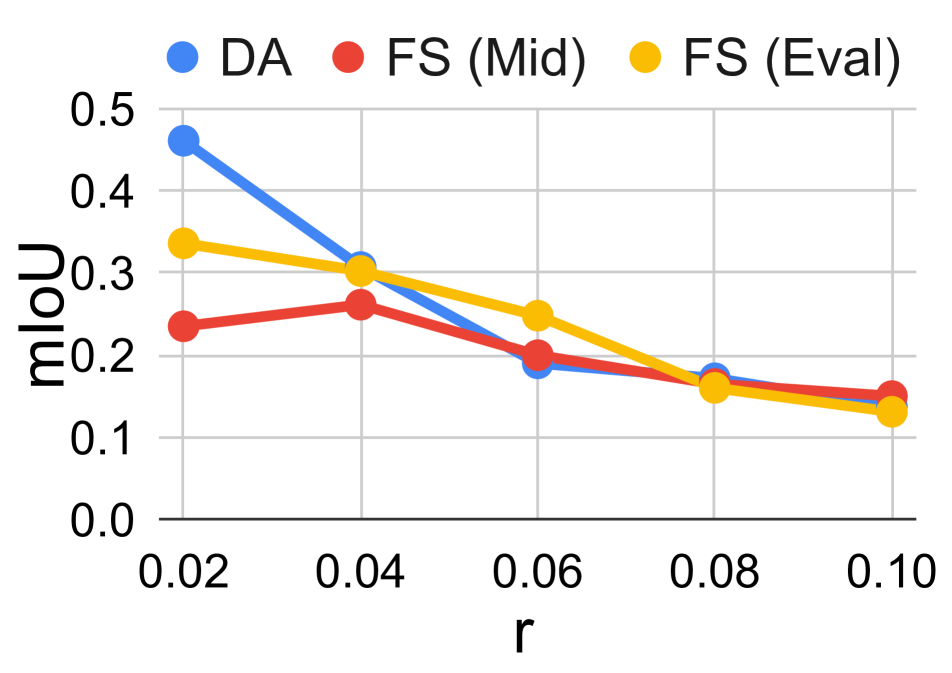
(b) GW radius $r$

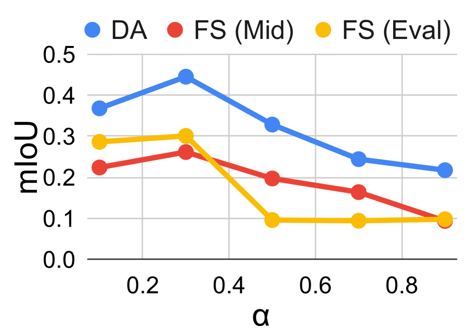
(c) GW weight $\alpha$

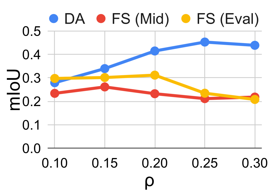
(d) Global temporal prior $\rho$

(e) Entropy reg. $\epsilon_{\text{train}}$

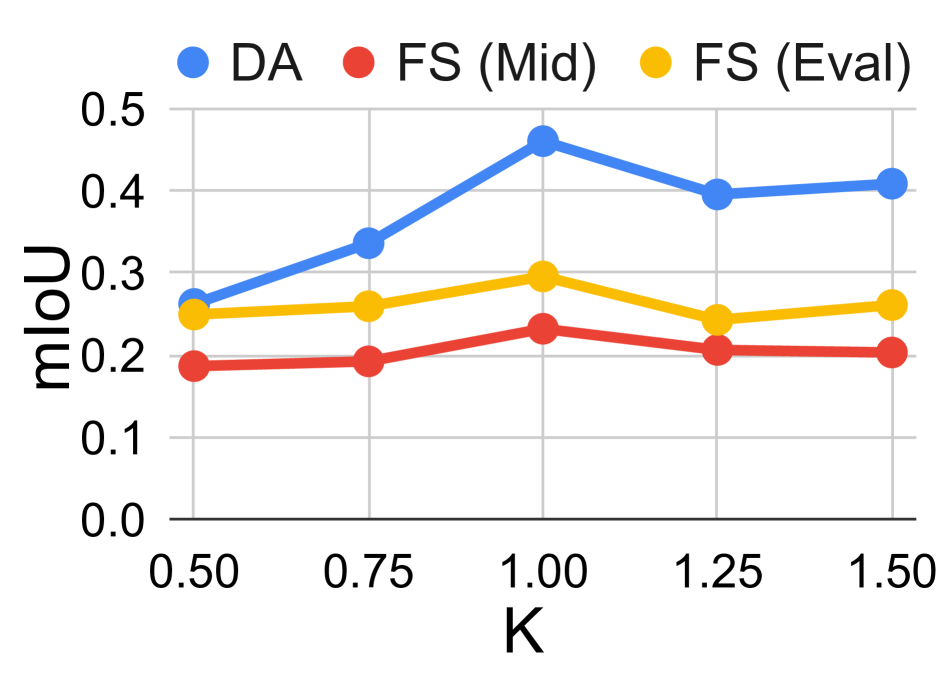
(f) Ratio of learned/true actions

Figure 8: Sensitivity analysis reporting mIoU-score on ASOT hyperparameters.

Appendix E Reproducibility

Our results in Tab. 1 and 2 were produced using one run, consistent with prior works in unsupervised action segmentation [22, 26, 23, 42, 36, 40]. To show the robustness of our methods, we used five runs on the 50 Salads and Desktop Assembly datasets with different random seeds. Differing random seeds impact the network initialization and sampling of batch indices for our training pipeline. We report the results of this experiment in Table (mean, std. err.) for the MoF metric (cf. Tab. 5).

Dataset	50 Salads (Mid)	50 Salads (Eval)	Desktop Ass.
MoF (%)	(43.0, 1.9)	(56.4, 2.8)	(62.9, 2.8)

Table 5: MoF results for five runs recorded as (mean, std. err.).

References

- [1] Hyemin Ahn and Dongheui Lee. Refining Action Segmentation With Hierarchical Video Representations. In Int. Conf. Comput. Vis., 2021.
- [2] Jean-Baptiste Alayrac, Piotr Bojanowski, Nishant Agrawal, Josef Sivic, Ivan Laptev, and Simon Lacoste-Julien. Unsupervised Learning From Narrated Instruction Videos. In IEEE Conf. Comput. Vis. Pattern Recog., June 2016.
- [3] Nicolas Aziere and Sinisa Todorovic. Multistage temporal convolution transformer for action segmentation. Image and Vision Computing, 2022.
- [4] Jonathan T. Barron and Ben Poole. The Fast Bilateral Solver. In Eur. Conf. Comput. Vis., 2016.
- [5] Nadine Behrmann, S. Alireza Golestaneh, Zico Kolter, Juergen Gall, and Mehdi Noroozi. Unified Fully and Timestamp Supervised Temporal Action Segmentation via Sequence to Sequence Translation. In Eur. Conf. Comput. Vis., 2022.
- [6] Mathilde Caron, Ishan Misra, Julien Mairal, Priya Goyal, Piotr Bojanowski, and Armand Joulin. Unsupervised Learning of Visual Features by Contrasting Cluster Assignments. In Adv. Neural Inform. Process. Syst., volume 33, 2020.
- [7] Min-Hung Chen, Baopu Li, Yingze Bao, Ghassan AlRegib, and Zsolt Kira. Action Segmentation With Joint Self-Supervised Temporal Domain Adaptation. In IEEE Conf. Comput. Vis. Pattern Recog., 2020.
- [8] Lenaic Chizat, Gabriel Peyré, Bernhard Schmitzer, and François-Xavier Vialard. Scaling Algorithms for Unbalanced Transport Problems. Mathematics of Computation, 87, 2016.
- [9] Marco Cuturi. Sinkhorn Distances: Lightspeed Computation of Optimal Transport. In Adv. Neural Inform. Process. Syst., volume 26, 2013.
- [10] Henri De Plaen, Pierre-François De Plaen, Johan A. K. Suykens, Marc Proesmans, Tinne Tuytelaars, and Luc Van Gool. Unbalanced Optimal Transport: A Unified Framework for Object Detection. In IEEE Conf. Comput. Vis. Pattern Recog., 2023.
- [11] Guodong Ding, Fadime Sener, and Angela Yao. Temporal Action Segmentation: An Analysis of Modern Techniques. IEEE Trans. Pattern Anal. Mach. Intell., 2023.
- [12] Zexing Du, Xue Wang, Guoqing Zhou, and Qing Wang. Fast and Unsupervised Action Boundary Detection for Action Segmentation. In IEEE Conf. Comput. Vis. Pattern Recog., 2022.
- [13] Yazan Abu Farha and Jurgen Gall. MS-TCN: Multi-Stage Temporal Convolutional Network for Action Segmentation. In IEEE Conf. Comput. Vis. Pattern Recog., 2019.
- [14] Dayan Guan, Jiaxing Huang, Aoran Xiao, and Shijian Lu. Domain Adaptive Video Segmentation via Temporal Consistency Regularization. In Int. Conf. Comput. Vis., 2021.
- [15] Yuchi Ishikawa, Seito Kasai, Yoshimitsu Aoki, and Hirokatsu Kataoka. Alleviating Over-segmentation Errors by Detecting Action Boundaries. In IEEE Wint. Conf. Applic. Comput. Vis., 2021.
- [16] Andrej Karpathy, George Toderici, Sanketh Shetty, Thomas Leung, Rahul Sukthankar, and Li Fei-Fei. Large-scale Video Classification with Convolutional Neural Networks. In IEEE Conf. Comput. Vis. Pattern Recog., 2014.
- [17] Will Kay, Joao Carreira, Karen Simonyan, Brian Zhang, Chloe Hillier, Sudheendra Vijayanarasimhan, Fabio Viola, Tim Green, Trevor Back, Paul Natsev, Mustafa Suleyman, and Andrew Zisserman. The Kinetics Human Action Video Dataset, 2017.
- [18] Abdelwahed Khamis, Russell Tsuchida, Mohamed Tarek, Vivien Rolland, and Lars Petersson. Earth Movers in The Big Data Era: A Review of Optimal Transport in Machine Learning, 2023.
- [19] Diederick P Kingma and Jimmy Ba. Adam: A method for stochastic optimization. In Int. Conf. Learn. Represent., 2015.
- [20] Krähenbühl, Philipp and Koltun, Vladlen. Efficient inference in fully connected crfs with gaussian edge potentials. In Adv. Neural Inform. Process. Syst., 2011.
- [21] Hilde Kuehne, Ali Arslan, and Thomas Serre. The Language of Actions: Recovering the Syntax and Semantics of Goal-Directed Human Activities. In IEEE Conf. Comput. Vis. Pattern Recog., 2014.
- [22] Anna Kukleva, Hilde Kuehne, Fadime Sener, and Jurgen Gall. Unsupervised Learning of Action Classes With Continuous Temporal Embedding. In IEEE Conf. Comput. Vis. Pattern Recog., June 2019.
- [23] Sateesh Kumar, Sanjay Haresh, Awais Ahmed, Andrey Konin, M. Zeeshan Zia, and Quoc-Huy Tran. Unsupervised Action Segmentation by Joint Representation Learning and Online Clustering. In IEEE Conf. Comput. Vis. Pattern Recog., June 2022.
- [24] Colin Lea, Michael D. Flynn, Rene Vidal, Austin Reiter, and Gregory D. Hager. Temporal Convolutional Networks for Action Segmentation and Detection. In IEEE Conf. Comput. Vis. Pattern Recog., 2017.
- [25] Peng Lei and Sinisa Todorovic. Temporal Deformable Residual Networks for Action Segmentation in Videos. In IEEE Conf. Comput. Vis. Pattern Recog., 2018.
- [26] Jun Li and Sinisa Todorovic. Action Shuffle Alternating Learning for Unsupervised Action Segmentation. In IEEE Conf. Comput. Vis. Pattern Recog., June 2021.
- [27] Mengyu Li, Jun Yu, Hongteng Xu, and Cheng Meng. Efficient Approximation of Gromov-Wasserstein Distance Using Importance Sparsification. Journal of Computational and Graphical Statistics, 2023.
- [28] Shijie Li, Yazan Abu Farha, Yun Liu, Ming-Ming Cheng, and Juergen Gall. MS-TCN++: Multi-Stage Temporal Convolutional Network for Action Segmentation. IEEE Trans. Pattern Anal. Mach. Intell., 2023.
- [29] Yanbin Liu, Linchao Zhu, Makoto Yamada, and Yi Yang. Semantic correspondence as an optimal transport problem. In IEEE Conf. Comput. Vis. Pattern Recog., 2020.
- [30] Gabriel Peyré, Marco Cuturi, and Justin Solomon. Gromov-Wasserstein Averaging of Kernel and Distance Matrices. In Int. Conf. Mach. Learn., Jun 2016.
- [31] Saquib Sarfraz, Naila Murray, Vivek Sharma, Ali Diba, Luc Van Gool, and Rainer Stiefelhagen. Temporally-Weighted Hierarchical Clustering for Unsupervised Action Segmentation. In IEEE Conf. Comput. Vis. Pattern Recog., 2021.
- [32] Paul-Edouard Sarlin, Daniel DeTone, Tomasz Malisiewicz, and Andrew Rabinovich. SuperGlue: Learning Feature Matching With Graph Neural Networks. In IEEE Conf. Comput. Vis. Pattern Recog., 2020.
- [33] Thibault Sejourne, Francois-Xavier Vialard, and Gabriel Peyré. The Unbalanced Gromov Wasserstein Distance: Conic Formulation and Relaxation. In Adv. Neural Inform. Process. Syst., 2021.
- [34] Zhengyang Shen, Jean Feydy, Peirong Liu, Ariel H Curiale, Ruben San Jose Estepar, Raul San Jose Estepar, and Marc Niethammer. Accurate Point Cloud Registration with Robust Optimal Transport. In Adv. Neural Inform. Process. Syst., 2021.
- [35] Sebastian Stein and Stephen J. McKenna. Combining Embedded Accelerometers with Computer Vision for Recognizing Food Preparation Activities. In ACM Int. Joi. Conf. Pervasive Ubiq. Comp., 2013.
- [36] Sirnam Swetha, Hilde Kuehne, Yogesh S Rawat, and Mubarak Shah. Unsupervised Discriminative Embedding For Sub-Action Learning in Complex Activities. In IEEE Int. Conf. Image Process., 2021.
- [37] Matthew Thorpe. Introduction to optimal transport, March 2018.
- [38] Alexis Thual, Quang Huy Tran, Tatiana Zemskova, Nicolas Courty, Rémi Flamary, Stanislas Dehaene, and Bertrand Thirion. Aligning individual brains with Fused Unbalanced Gromov-Wasserstein. In Adv. Neural Inform. Process. Syst., 2022.
- [39] Vayer Titouan, Nicolas Courty, Romain Tavenard, Chapel Laetitia, and Rémi Flamary. Optimal transport for structured data with application on graphs. In Int. Conf. Mach. Learn., Jun 2019.
- [40] Quoc-Huy Tran, Ahmed Mehmood, Muhammad Ahmed, Muhammad Naufil, Anas Zafar, Andrey Konin, and M. Zeeshan Zia. Permutation-Aware Action Segmentation via Unsupervised Frame-to-Segment Alignment, 2023.
- [41] Titouan Vayer, Laetitia Chapel, Remi Flamary, Romain Tavenard, and Nicolas Courty. Fused Gromov-Wasserstein Distance for Structured Objects. Algorithms, 13, 2020.
- [42] Rosaura G. VidalMata, Walter J. Scheirer, Anna Kukleva, David Cox, and Hilde Kuehne. Joint Visual-Temporal Embedding for Unsupervised Learning of Actions in Untrimmed Sequences. In IEEE Wint. Conf. Applic. Comput. Vis., 2021.
- [43] Hongteng Xu, Dixin Luo, Hongyuan Zha, and Lawrence Carin Duke. Gromov-Wasserstein Learning for Graph Matching and Node Embedding. In Int. Conf. Mach. Learn., 2019.
- [44] Fangqiu Yi, Hongyu Wen, and Tingting Jiang. Asformer: Transformer for action segmentation. In Brit. Mach. Vis. Conf., 2021.
- [45] Asano YM., Rupprecht C., and Vedaldi A. Self-labelling via simultaneous clustering and representation learning. In Int. Conf. Learn. Represent., 2020.