Probing Stochastic Ultralight Dark Matter with Space-based Gravitational-Wave Interferometers

Abstract

Ultralight particles are theoretically well-motivated dark matter candidates. In the vicinity of the solar system, these ultralight particles are described as a superposition of plane waves, resulting in a stochastic field with amplitude fluctuations on scales determined by the velocity dispersion of dark matter. In this work, we systematically investigate the sensitivity of space-based gravitational-wave interferometers to the stochastic ultralight dark matter field within the frequentist framework. We derive the projected sensitivity of a single detector using the time-delay interferometry and find that the stochastic effect will only diminish the performance of the detector marginally, unlike searches in other contexts where significant reductions are found. Furthermore, we explore the sensitivity of detector network in two typical configurations. We find that the well-separated configuration, where the distance between two detectors exceeds the coherence length of dark matter, is the optimal choice for ultralight dark matter detection due to a less chance of missing signal. This contrasts with the detection of stochastic gravitational-wave background, where the co-located and co-aligned configuration is preferred. Our results may provide useful insights for potential joint observations involving gravitational-wave detectors like LISA, Taiji and TianQin.

I Introduction

According to the standard model of cosmology $\Lambda$CDM, dark matter (DM) makes up the dominant part of matter in the universe, but its particle nature still remains mystery. Ultralight bosonic particles, like axion Peccei and Quinn (1977); Weinberg (1978); Wilczek (1978); Preskill et al. (1983); Abbott and Sikivie (1983); Dine and Fischler (1983), dilaton Damour and Polyakov (1994a, b); Capozziello and De Laurentis (2011) and dark photon Nelson and Scholtz (2011); Graham et al. (2016); Ema et al. (2019); Ahmed et al. (2020); Kolb and Long (2021), are viable candidates of DM, which not only have strong theoretical motivation but also can mitigate tensions of $\Lambda$CDM on small scales de Blok (2010); Boylan-Kolchin et al. (2011); Bullock and Boylan-Kolchin (2017); Tulin and Yu (2018). These ultralight particles typically have mass below $10$ eV Hu et al. (2000); Hui et al. (2017); Hui (2021), which implies that their occupation number in a de Broglie volume is numerous if they contribute a non-negligible fraction of the local DM. Therefore, quantum fluctuations are suppressed and these ultralight particles can be effectively described by classical waves. These waves with random initial phases travel at different velocities and interfere with each other, resulting in a stochastic field whose amplitude evolves randomly on the time scale (coherence time) and spatial scale (coherence length) determined by the velocity dispersion of DM Derevianko (2018); Foster et al. (2018, 2021).

Numerous experiments have been conducted or proposed, spanning different mass bands and exploring diverse phenomenological aspects of ultralight DM (ULDM) Van Tilburg et al. (2015); Arvanitaki et al. (2016); Hees et al. (2016); Geraci et al. (2019); Hochberg et al. (2016); Fayet (2018); Xia et al. (2021); An et al. (2023, 2021); Rogers and Peiris (2021); Fedderke and Mathur (2023); Arvanitaki and Dubovsky (2011); Cardoso et al. (2018); Davoudiasl and Denton (2019); Chen et al. (2020); Liang et al. (2023); Kim (2023); Khmelnitsky and Rubakov (2014); Wu et al. (2023); Sun et al. (2022); Cao and Tang (2023); Kim and Mitridate (2024); Luu et al. (2024). For instance, if ULDM couples with the Standard Model (SM) within the low-energy effective action, it could mediate an additional force that is potentially detectable in the fifth-force experiments Adelberger et al. (2003). Besides, this force is generally composition-dependent Damour and Donoghue (2010), i.e. its strength varies among different materials, and may induce violations of equivalence principle (EP), which can be probed by EP tests such as the Lunar Laser Ranging Williams et al. (2004); WILLIAMS et al. (2009), experiments conducted by the Eöt-Wash group Schlamminger et al. (2008); Wagner et al. (2012), and the MICROSCOPE mission et al. (2017); et al (2022).

ULDM can also imprint observable signatures in gravitational wave (GW) interferometers by exerting position-dependent oscillatory force on test masses Arvanitaki et al. (2018); Pierce et al. (2018); Grote and Stadnik (2019); Vermeulen et al. (2021). Constraints from both ground-based GW detectors like LIGO and Virgo Abbott et al. (2016) and spacecraft LISA-Pathfinder et al (2018) have been obtained Guo et al. (2019); Fukusumi et al. (2023); Miller and Mendes (2023), and projected sensitivities of space-based GW detectors such as LISA et al (2017), Taiji Hu and Wu (2017) and TianQin Luo et al. (2016) have also been derived Pierce et al. (2018); Morisaki and Suyama (2019); Yu et al. (2023), which shows the remarkable ability of GW detectors on exploring unknown parameter space. In the future, GW detectors are expected to improve current constraints by several times for dilaton-like scalar fields, and several orders of magnitude more if the vector field couples with the baryon number or baryon minus lepton number. In addition, it is worth mentioning that GW detectors will probe a different direction in the space of coupling parameters, complementing the EP tests. As the test masses in GW detectors are made of the same material, they are insensitive to the composition-dependent effects. As we will see, for the general parametrized dilaton interaction GW detectors will constraint the composition-independent coupling parameter $d^{*}_{g}$. In contrast, the EP tests are sensitive to the composition-dependent effects and give direct constraints on linear combinations of coupling parameters involving $d^{*}_{g}$ Bergé et al. (2018).

In most of previous works, the authors usually treat ULDM field as deterministic and neglect its stochastic property in deriving sensitivity of detectors for simplicity. However, it has been pointed out that accounting for the stochastic nature is crucial for interpreting the experiment results and deriving the appropriate constraints Centers et al. (2021); Lisanti et al. (2021).

In this work, we investigate the sensitivity of space-based GW interferometers to the stochastic ULDM field systematically within the frequentist framework, accounting for its stochastic nature through a general likelihood approach. While we take scalar field as an example, our method can be readily extend to vector and tensor fields. We first derive the sensitivity of a single detector using time-delay interferometry (TDI) Armstrong et al. (1999); Estabrook et al. (2000); Tinto and Dhurandhar (2021) and find that the stochastic effect will only mildly weaken the sensitivity, in contrast to other searches where the reductions are notable. We then investigate the sensitivity of detector network in two typical configurations using the general likelihood formalism. We introduce the overlap reduction function for ULDM, which measures correlation between ULDM signals in different detectors. We find that the well-separated configuration, where detectors are at distance exceeding the coherence length of ULDM field, outperforms the co-aligned and co-located configuration, since detectors in the well-separated configuration will probe independent patches of the stochastic field and reduce the probability of missing ULDM signal. This highlights the advantage of the well-separated configuration for ULDM detection, contrasting with the detection of stochastic gravitational wave background (SGWB) Allen and Romano (1999); Romano and Cornish (2017) where the co-aligned and co-located configuration is favored for its ability to enhance the signal-to-noise ratio through signal correlation.

This paper is organized as follows. In II, we derive and summarize some useful results of ULDM. In III, we specify the interactions between the ULDM and the SM and derive the power spectral density (PSD) of the ULDM signal in TDI channels. In IV.1, we derive the sensitivity of a single detector. The sensitivity of network is explored in IV.2, where we also compare ULDM detection with SGWB detection. Finally, we conclude in V.

In this paper, we use natural units ($c=\hbar=1$) unless explicitly stated otherwise.

II Theoretical Framework for Ultra-Light Dark Matter

In this section, we present the theoretical framework of ULDM and clarify notations for our later discussions. Similar treatments can be found in Refs. Derevianko (2018); Foster et al. (2018); Gramolin et al. (2022); Hui et al. (2021); Hui (2021); Nakatsuka et al. (2022).

II.1 The local ULDM field

The local ULDM filed $\Phi(t,\mathbf{x})$ can be described as a superposition of monochromatic plane waves

$$\Phi(x)=\sum_{\mathbf{v}}\frac{\sqrt{2\rho/N}}{m}\;e^{i\left(\omega t-\mathbf{k}\cdot\mathbf{x}+\theta_{\mathbf{v}}\right)},$$ (1)

where $\omega=m(1+v^{2}/2)$, $\mathbf{k}=m\mathbf{v}$, $m$ is the mass of ULDM particles, $\theta_{\mathbf{v}}$s are random phases drawn independently from the $[0,2\pi)$ uniform distribution, $\rho$  is the local energy density of DM, and $N$ denotes the total number of ULDM particles in the vicinity.

We decompose the sum over velocity in Eq. (1) into two steps,

$$\Phi(x)=\sum_{\mathbf{v}_{i}}\sum_{\mathbf{v}\in[\mathbf{v}_{i},\mathbf{v}_{i}+\Delta\mathbf{v})}\frac{\sqrt{2\rho/N}}{m}\;e^{i\left(\omega t-\mathbf{k}\cdot\mathbf{x}+\theta_{\mathbf{v}}\right)}.$$ (2)

We first sum up the components in a small velocity interval $\Delta\mathbf{v}$, which is small enough that we can ignore the difference between their velocities,

$$\sum_{\mathbf{v}\in[\mathbf{v}_{i},\mathbf{v}_{i}+\Delta\mathbf{v})}\frac{\sqrt{2\rho/N}}{m}\;e^{i\left(\omega t-\mathbf{k}\cdot\mathbf{x}+\theta_{\mathbf{v}}\right)}\simeq\frac{\sqrt{2\rho/N}}{m}e^{i\left[m(1+v_{i}^{2}/2)t-\mathbf{k}_{i}\cdot\mathbf{x}\right]}\sum_{\mathbf{v}\in[\mathbf{v}_{i},\mathbf{v}_{i}+\Delta\mathbf{v})}e^{i\theta_{\mathbf{v}}}.$$ (3)

The sum over random phases is equivalent to a random walk in the complex plane and can be written as

$$\sum_{\mathbf{v}\in[\mathbf{v}_{j},\mathbf{v}_{j}+\Delta\mathbf{v})}e^{i\theta_{\mathbf{v}}}=\beta_{j}e^{i\theta_{j}},$$ (4)

where $\theta_{j}$ is again a random phase distributed uniformly in $[0,2\pi)$, and $\beta_{j}$ a random variable governed by the Rayleigh distribution

$$P\left(\beta_{j}\right)=\frac{2\beta_{j}}{N_{j}}e^{-\beta^{2}_{j}/N_{j}}.$$ (5)

$N_{j}$ is the number of terms in the sum $\sum_{\mathbf{v}\in[\mathbf{v}_{i},\mathbf{v}_{i}+\Delta\mathbf{v})}$ or equivalently the number of ULDM particles in the velocity interval $[\mathbf{v}_{j},\mathbf{v}_{j}+\Delta\mathbf{v})$ given by

$$N_{j}=N\cdot\Delta_{j},\quad\Delta_{j}\equiv d^{3}v\;f(\mathbf{v}_{j}),$$ (6)

with $f(\mathbf{v})$ the normalized velocity distribution of DM.

Gathering the above results and rescaling $\beta_{j}$ by $\sqrt{N_{j}/2}$ to get rid of the $N_{j}$ dependence in Eq. (5), Eq. (1) can be simplified to the form

$$\Phi(x)=\frac{\sqrt{\rho}}{m}\sum_{\mathbf{v}_{j}}\sqrt{\frac{N_{j}}{N}}\;\beta_{j}e^{i\left(\omega_{j}t-\mathbf{k}_{j}\cdot\mathbf{x}+\theta_{j}\right)}=\frac{\sqrt{\rho}}{m}\sum_{\mathbf{v}_{j}}\sqrt{\Delta_{j}}\;\beta_{j}e^{i\left(\omega_{j}t-\mathbf{k}_{j}\cdot\mathbf{x}+\theta_{j}\right)},$$ (7)

or using $n,l$ to label the magnitude and direction of velocity, $\mathbf{v}=v_{n}\hat{e}_{l}$ ($|\hat{e}_{l}|=1$),

$$\Phi(x)=\frac{\sqrt{\rho}}{m}\sum_{n}\sum_{l}\sqrt{\Delta_{nl}}\;\beta_{nl}e^{i\left(\omega_{nl}t-\mathbf{k}_{nl}\cdot\mathbf{x}+\theta_{nl}\right)}.$$ (8)

Figure. 1 is a 3D snapshot of $\Phi(x)$ generating with Eq. (8). As illustrated, $\Phi(x)$ fluctuates stochastically on spatial scale $\lambda_{c}$, which is the coherence length of ULDM field defined in Eq. (18), and the field values at two points separated by a distance greater than $\lambda_{c}$ are uncorrelated.

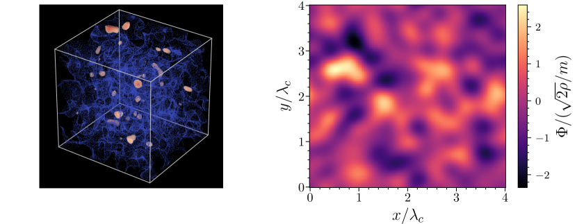
Figure 1: A realization of ULDM field $\Phi(t=0,\mathbf{x})$. (Left) The spatial distribution of density $\rho=\Phi^{2}$, with high-density regions in red and low-density regions in blue. (Right) A 2D slice of $\Phi(x)$ with constant $t$ and $z$. The patterns, arising from interference between waves, have a typical size $\lambda_{c}^{3}$. When $|\mathbf{x}_{1}-\mathbf{x}_{2}|\gg\lambda_{c}$, the field values $\Phi(t,\mathbf{x}_{1})$ and $\Phi(t,\mathbf{x}_{2})$ are independent from each other.

The spatial derivative of $\Phi(x)$ can be readily obtained by differentiating Eq. (8),

$$\nabla\Phi(x)=-i\sqrt{\rho}\sum_{n}\sum_{l}\sqrt{\Delta_{nl}}v_{n}\beta_{nl}e^{i\left(\omega_{nl}t-\mathbf{k}_{nl}\cdot\mathbf{x}+\theta_{nl}\right)}\hat{e}_{l}.$$ (9)

II.2 Two-point correlation function

ULDM field has a stochastic nature, and its statistical properties are encoded entirely in the correlation function. We calculate the two-point correlation function for ULDM from Eq. (8) directly (see Appendix A for details)

$$R_{\Phi}(\tau,\mathbf{d}):=\langle\Phi(x)\Phi(x^{\prime})\rangle=\frac{\rho}{m^{2}}\int d^{3}v\;f(\mathbf{v})\;\cos\left[m\left(1+\frac{v^{2}}{2}\right)\tau-m\mathbf{v}\cdot\mathbf{d}\right],$$ (10)

where $\tau\equiv t^{\prime}-t$, $\mathbf{d}\equiv\mathbf{x}^{\prime}-\mathbf{x}$, and $\langle\cdots\rangle$ denotes ensemble average. It is easy to check that

$$\left\langle\Phi^{2}(x)\right\rangle=\frac{\rho}{m^{2}}\int d^{3}vf(\mathbf{v})=\frac{\rho}{m^{2}}\;,$$ (11)

where we use the normalization condition of velocity distribution. Eq. (11) indicates that $\Phi$ constitutes the entire local DM content.

Correlation functions between the field and its spatial derivative $R_{i}(\tau,\mathbf{d})\equiv\langle\Phi(x)\partial^{\prime}_{i}\Phi(x^{\prime})\rangle$ and between spatial derivatives themselves $R_{ij}(\tau,\mathbf{d})\equiv\langle\partial_{i}\Phi(x)\partial^{\prime}_{j}\Phi(x^{\prime})\rangle$ can be derived from Eq. (8, 9) through straightforward but tedious calculation. However, there is a simple way to derive them. We note that $R_{ij}(\tau,\mathbf{d})\equiv\langle\partial_{i}\Phi(x)\partial^{\prime}_{j}\Phi(x^{\prime})\rangle=\partial_{i}\partial^{\prime}_{j}\langle\Phi(x)\Phi(x^{\prime})\rangle=-\partial^{\mathbf{d}}_{i}\partial^{\mathbf{d}}_{j}R_{\Phi}(\tau,\mathbf{d})$ with the superscript $\mathbf{d}$ indicating that the derivative acts on $\mathbf{d}$. Combining with Eq. (10), we have

$$R_{i}(\tau,\mathbf{d}) =\frac{\rho}{m}\int d^{3}v\;f(\mathbf{v})v_{i}\;\sin\left[m\left(1+\frac{v^{2}}{2}\right)\tau-m\mathbf{v}\cdot\mathbf{d}\right],$$ (12)

$$R_{ij}(\tau,\mathbf{d}) =\rho\int d^{3}v\;f(\mathbf{v})v_{i}v_{j}\;\cos\left[m\left(1+\frac{v^{2}}{2}\right)\tau-m\mathbf{v}\cdot\mathbf{d}\right].$$ (13)

II.3 Power spectral density of ULDM field

Due to the stochastic nature of ULDM field, the detector signal induced by its oscillation is also stochastic, with its properties characterized statistically by the power spectral density (PSD). As we will see, the signal PSD is related to the PSD of ULDM through the reponse function of detector. The two-sided PSD of ULDM is defined as the Fourier transform of the correlation function,

$$\begin{split}S_{\Phi}(f,\mathbf{d})&:=\int^{\infty}_{-\infty}d\tau\;e^{-i2\pi f\tau}\;R_{\Phi}(\tau,\mathbf{d})\\ &=\frac{\rho}{m^{2}}\int^{\infty}_{-\infty}d\tau\;e^{-i2\pi f\tau}\times\int dvv^{2}\int d\hat{\Omega}\;f(\mathbf{v})\;\cos\left[m\left(1+\frac{v^{2}}{2}\right)\tau-m\mathbf{v}\cdot\mathbf{d}\right]\\ &=\frac{\pi\rho}{m^{3}}v_{f}\int d\hat{\Omega}\;f(v_{f}\hat{\Omega})\;e^{-imv_{f}\hat{\Omega}\cdot\mathbf{d}},\end{split}$$ (14)

where $v_{f}=\sqrt{2(f/f_{c}-1)}$, $f_{c}=m/(2\pi)$, and we neglect the negative frequency part. From Eq. (14), we observe that $S_{\Phi}(f,\mathbf{d})$ has a structure closely related to the phase space structure of DM.

If the velocity distribution is isotropic, i.e.$~{}f(\mathbf{v})=f(v)$, then the directional integral in Eq. (14) can be performed analytically and we have

$$S^{\text{iso}}_{\Phi}(f,\mathbf{d})=\frac{\pi\rho}{m^{3}}f(v_{f})v_{f}\int d\hat{\Omega}\;e^{-imv_{f}\hat{\Omega}\cdot\mathbf{d}}=\frac{4\pi^{2}\rho}{m^{3}}v_{f}f(v_{f})\;\text{sinc}(mv_{f}d),$$ (15)

where $d\equiv|\mathbf{d}|$ and $\text{sinc}(x)\equiv\sin(x)/x$. In cases with a general velocity distribution, analytic results are not available and the integral needs to be performed numerically.

Another useful quantity is $S_{\Phi}(f,\hat{k})$, the “skymap” of ULDM field, which is the projection of $S_{\Phi}(f,\mathbf{d})$ onto the unit direction vector $\hat{k}$. We derive the explicit expression of $S_{\Phi}(f,\hat{k})$ in Appendix C.

III Detect ULDM with Space-based Gravitational-Wave Interferometers

III.1 Response of interferometer to ULDM

Now, we discuss how ULDM is responded in a GW laser interferometer in space. We first define some useful quantities for ULDM with mass $m$, including Compton frequency, coherence time, and coherence length,

$$f_{c} =\frac{mc^{2}}{2\pi\hbar}\approx 2.42\times\left(\frac{m}{10^{-17}~{}\text{eV}}\right)~{}\text{mHz},$$ (16)

$$\tau_{c} =\frac{\hbar}{mc^{2}\sigma^{2}}\approx 6.58\times 10^{7}\left(\frac{10^{-17}~{}\text{eV}}{m}\right)~{}\text{s},$$ (17)

$$\lambda_{c} =\frac{\hbar}{m\sigma c}\approx 1.97\times 10^{10}\left(\frac{10^{-17}~{}\text{eV}}{m}\right)~{}\text{km},$$ (18)

where $\sigma\sim 10^{-3}$ is the velocity dispersion of local DM. The sensitivity band of space-based GW interferometers, such as LISA and Taiji, is around several mHz, which corresponds to the ULDM with a mass around $10^{-17}$ eV. Consequently, the ULDM will have $\tau_{c}>T\sim 3\times 10^{7}~{}\text{s}$  and $\lambda_{c}\gg L\sim 10^{6}~{}\text{km}$, where $T$ is the total observation time and $L$ is the armlength of interferometer. This indicates that LISA will not have sufficient frequency resolution to resolve the spectrum $S_{\Phi}$, which has a characteristic width of about $1/\tau_{c}$ in the Fourier domain, and we can treat the ULDM as monochromatic. Thus, Eq. (9) can be approximated by

$$\nabla\Phi(x)\simeq-i\sqrt{\rho}e^{imt}\sum_{n}\sum_{l}\sqrt{\Delta_{nl}}v_{n}\beta_{nl}e^{-i\left(\mathbf{k}_{nl}\cdot\mathbf{x}-\theta_{nl}\right)}\hat{e}_{l}.$$ (19)

To proceed, we need to specify the coupling between ULDM and the SM. Here, we illustrate the physical effects with scalar ULDM, which is coupled with test mass through the trace of energy-momentum tensor. Note that our methodology can be readily extended to vector and tensor ULDM with different couplings. The action of test mass is given by Morisaki and Suyama (2019)

$$S=-\int m(\Phi)\sqrt{-\eta_{\mu\nu}dx^{\mu}dx^{\nu}},$$ (20)

from which we can obtain the non-relativistic equation of motion of test mass,

$$\frac{d^{2}\mathbf{x}}{dt}\simeq-k\alpha(\Phi)\nabla\Phi,\qquad\alpha(\Phi)\equiv\frac{\partial\ln\left[\kappa m(\Phi)\right]}{\partial(\kappa\Phi)},$$ (21)

where $\kappa\equiv\sqrt{4\pi G}$ is the inverse of the Planck mass. The dimensionless factor $\alpha(\Phi)$ is determined by the interactions between the ULDM and the SM. In this work, we consider the general parametrized interaction Damour and Donoghue (2010),

$$\mathcal{L}_{\Phi-\text{SM}}=\kappa\Phi\left[\frac{d_{e}}{4e^{2}}F_{\mu\nu}F^{\mu\nu}-\frac{d_{g}\beta_{3}}{2g_{3}}G^{A}_{\mu\nu}G^{A\mu\nu}-\sum_{i=e,u,d}(d_{m_{i}}+\gamma_{m_{i}}d_{g})m_{i}\bar{\psi}_{i}\psi_{i}\right],$$ (22)

where $d_{g}$, $d_{e}$ denote for the couplings of the ULDM to the electromagnetic and gluonic field terms, $d_{m_{i}}$ ($i=e,u,d$) the couplings to the fermionic mass terms, $F_{\mu\nu}$, $G^{A}_{\mu\nu}$ are the electromagnetic and gluon field strength tensors, $e$ the electron charge, $g_{3}$ the $\text{SU}(3)$ gauge coupling, $\beta_{3}$ the QCD beta function, and $\gamma_{m_{i}}$ the anomalous dimensions of fermion. Around the energy scale of nuclei, $\alpha(\Phi)$ is approximately given by Damour and Donoghue (2010)

$$\alpha(\Phi)\simeq d^{*}_{g}\simeq d_{g}+0.093(d_{\hat{m}}-d_{g}),\qquad d_{\hat{m}}\equiv\frac{d_{m_{d}}m_{d}+d_{m_{u}}m_{u}}{m_{d}+m_{u}}.$$ (23)

The velocity variation of test mass induced by the ULDM oscillation can be obtained by integrating Eq. (21),

$$\frac{d\mathbf{x}}{dt}=-\frac{\lambda}{im}\nabla\Phi,$$ (24)

where $\lambda\equiv\kappa\alpha(\Phi)\simeq\kappa d^{*}_{g}$. Then, the frequency modulation of laser in a single link due to the velocity variation (Doppler shift) is

$$\eta_{rs}(t)\equiv\frac{\delta\nu}{\nu_{0}}=-\hat{n}_{rs}\cdot\left(\frac{d\mathbf{x}}{dt}\bigg{|}_{t,\mathbf{x}_{r}}-\frac{d\mathbf{x}}{dt}\bigg{|}_{t-L,\mathbf{x}_{s}}\right)=\frac{\lambda}{im}\hat{n}_{rs}\cdot\left(\nabla\Phi\bigg{|}_{t,\mathbf{x}_{r}}-\nabla\Phi\bigg{|}_{t-L,\mathbf{x}_{s}}\right),$$ (25)

where $\hat{n}_{rs}$ is the unit vector pointing from the position of the sender spacecraft $\mathbf{x}_{s}$ to the receiver spacecraft $\mathbf{x}_{r}$. Substitute Eq. (19) into Eq. (25), we have

$$\eta_{rs}(t) =-\lambda\frac{\sqrt{\rho}}{m}\hat{n}_{rs}\cdot\left[e^{imt}\sum_{n,l}\sqrt{\Delta_{nl}}v_{n}\beta_{nl}e^{-i\left(\mathbf{k}_{nl}\cdot\mathbf{x}_{r}-\theta_{nl}\right)}\hat{e}_{l}\right.$$ (26)

$$\quad\quad\quad\quad\quad\quad\quad\quad\left.-e^{im(t-L)}\sum_{p,q}\sqrt{\Delta_{pq}}v_{p}\beta_{pq}e^{-i\left(\mathbf{k}_{pq}\cdot\mathbf{x}_{s}-\theta_{pq}\right)}\hat{e}_{q}\right]$$

$$\simeq-\lambda\frac{\sqrt{\rho}}{m}e^{imt}\left(1-e^{-imL}\right)\sum_{n,l}\sqrt{\Delta_{nl}}v_{n}\beta_{nl}e^{-i\left(\mathbf{k}_{nl}\cdot\mathbf{x}_{r}-\theta_{nl}\right)}\hat{e}_{l}\cdot\hat{n}_{rs}\;,$$

where we have used $L\ll\lambda_{c}$ in the last line.

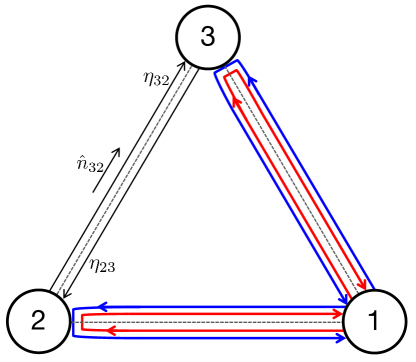
Figure 2: Illustration of the equilateral triangular configuration of space-based GW detectors such as LISA, Taiji and TianQin. The red and blue lines indicate the synthetic light path of $X$ channel.

From the single-link response Eq. (26), we can then construct the round-trip signal $\xi_{rsr}(t)$, Michelson interference signal $M(t)$ and signal $X(t)$. Their expressions are listed below:

$$\xi_{rsr}(t) =\eta_{rs}(t)+\eta_{sr}(t-L)$$

$$\simeq-\lambda\frac{\sqrt{\rho}}{m}e^{imt}\left(1-e^{-imL}\right)^{2}\sum_{n,l}\sqrt{\Delta_{nl}}v_{n}\beta_{nl}e^{-i\left(\mathbf{k}_{nl}\cdot\mathbf{x}_{r}-\theta_{nl}\right)}\hat{e}_{l}\cdot\hat{n}_{rs},$$ (27)

$$M(t) =\xi_{121}(t)-\xi_{131}(t)$$

$$\simeq-\lambda\frac{\sqrt{\rho}}{m}e^{imt}\left(1-e^{-imL}\right)^{2}\sum_{n,l}\sqrt{\Delta_{nl}}v_{n}\beta_{nl}e^{-i\left(\mathbf{k}_{nl}\cdot\mathbf{x}_{1}-\theta_{nl}\right)}\left[\hat{e}_{l}\cdot(\hat{n}_{12}-\hat{n}_{13})\right],$$ (28)

$$X(t) =\left[\xi_{131}(t)+\xi_{121}(t-2L)\right]-\left[\xi_{121}(t)+\xi_{131}(t-2L)\right]$$

$$\simeq\left(1-e^{-2imL}\right)M(t)\;.$$ (29)

III.2 The power spectral density of ULDM signal

The ULDM signal is characterized statistically by the corresponding PSD. For the Michelson interference, the auto-correlation function is given by

$$R_{M}(\tau)\equiv\langle M(t)M(t+\tau)\rangle=\frac{16\rho\lambda^{2}}{m^{2}}\sin^{4}\left(\frac{mL}{2}\right)I_{\text{vel}}\cos\left(m\tau\right),$$ (30)

where the velocity integral $I_{\text{vel}}$ is defined as

$$I_{\text{vel}}\equiv\int d^{3}v\;f(\mathbf{v})\left[\mathbf{v}\cdot(\hat{n}_{12}-\hat{n}_{13})\right]^{2}.$$ (31)

Due to Eq. (III.1), the auto-correlation function of $X$ follows that

$$R_{X}(\tau)\equiv\langle X(t)X(t+\tau)\rangle=4\sin^{2}\left(mL\right)R_{M}(\tau).$$ (32)

The two-sided PSDs are obtained by Fourier transforming the auto-correlation function. The results are

$$S_{M}(f)=\frac{8\rho\lambda^{2}}{m^{2}}\sin^{4}\left(\frac{mL}{2}\right)I_{\text{vel}}\times\delta\left(f-f_{c}\right)\simeq\frac{2\rho\lambda^{2}}{\pi^{2}f^{2}}\sin^{4}\left(\pi fL\right)I_{\text{vel}}T,\quad f=f_{c}\;,$$ (33)

where we replace the $\delta$ function by the finite observation time $T$, and similarly

$$S_{X}(f)=4\sin^{2}\left(2\pi fL\right)S_{M}(f),\quad f=f_{c}\;.$$ (34)

From Eqs. (33, 34), it is clear that ULDM signal will manifest as a monochromatic signal at the Compton frequency $f_{c}$ with its intensity being proportional to $T$.

For later convenience, we rewrite Eqs. (33, 34) in terms of the response function of TDI channel Yu et al. (2023) and $S_{\Phi}(f,\mathbf{d})$. Observe that for $T\ll\tau_{c}$, we have

$$\frac{\nabla_{\mathbf{d}}}{-im}S_{\Phi}(f,\mathbf{d})\simeq\frac{\rho}{m^{2}}\int d^{3}v\;\mathbf{v}f(\mathbf{v})e^{-im\mathbf{v}\cdot\mathbf{d}}\times\frac{1}{2}\delta\left(f-f_{c}\right).$$ (35)

This suggests that we can replace $\mathbf{v}$ in Eq. (31) by the operator $\nabla_{\mathbf{d}}/(-im)$ and Eq. (33) can be rewritten as

$$S_{M}(f)=\lambda^{2}\big{[}\Gamma_{M}(f)S_{\Phi}(f,\mathbf{d})\big{]}\Big{|}_{\mathbf{d}=\mathbf{0}},$$ (36)

where

$$\Gamma_{M}(f)=16\sin^{4}\left(\pi fL\right)\left[(\hat{n}_{12}-\hat{n}_{13})\cdot\frac{\nabla_{\mathbf{d}}}{-im}\right]^{2},$$ (37)

which is just the square of modulus of the response function of Michelson interference derived in Yu et al. (2023). In general, the two-sided PSD of the ULDM signal in a general TDI channel $O$ can be written as

$$S_{O}(f)=\lambda^{2}\big{[}\Gamma_{O}(f)S_{\Phi}(f,\mathbf{d})\big{]}\Big{|}_{\mathbf{d}=\mathbf{0}},$$ (38)

where $\Gamma_{O}$ is the square of modulus of the response function of $O$ channel.

III.3 Velocity integral

The information about phase space of DM is encoded into the velocity integral $I_{\text{vel}}$. Here, we list the results of integral for three interested velocity distributions for later use.

• The isotropic Maxwellian distribution:

  $$f(\mathbf{v})=\frac{1}{(2\pi\sigma^{2})^{3/2}}e^{-\frac{v^{2}}{2\sigma^{2}}},$$ (39)

  with variance $\langle v^{2}\rangle=3\sigma^{2}$, and $I^{\text{iso}}_{\text{vel}}=\sigma^{2}$.

• The $\delta$ distribution corresponds to the monochromatic plane waves:

  $$f(\mathbf{v})=\frac{1}{4\pi\sigma^{2}}\delta\left(v-\sigma\right),$$ (40)

  with variance $\langle v^{2}\rangle=\sigma^{2}$, and $I^{\delta}_{\text{vel}}=\sigma^{2}/3$.

• The boosted Maxwellian distribution in the Solar System Barycenter frame:

  $$f(\mathbf{v})=\frac{1}{(2\pi\sigma^{2})^{3/2}}e^{-\frac{(\mathbf{v}+\mathbf{v}_{\odot})^{2}}{2\sigma^{2}}},$$ (41)

  with $I^{\odot}_{\text{vel}}=\sigma^{2}(1+\cos^{2}\iota)$, where $\iota$ is the angle between $\mathbf{v}_{\odot}$ and $\hat{n}_{12}-\hat{n}_{13}$. $\mathbf{v}_{\odot}$ is the velocity of the solar system in the galactic rest frame and $|\mathbf{v}_{\odot}|\simeq\sigma$.

Note that the relative magnitudes of the velocity integrals: $I^{\odot}_{\text{vel}}\geq I^{\text{iso}}_{\text{vel}}>I^{\delta}_{\text{vel}}$. Also, besides the isotropic background contribution $\sigma^{2}$, $I^{\odot}_{\text{vel}}$ get an additional term $\sigma^{2}\cos^{2}\iota$ due to the boost of reference frame. When $\iota=0$ or $\pi$, i.e. $\hat{n}_{12}-\hat{n}_{13}$ aligned or anti-aligned with the velocity of Sun in the galactic rest frame, the signal power will get a factor of 2 enhancement compared to the isotropic case.

IV Sensitivity

IV.1 Sensitivity of A Single Detector

Since ULDM signal is contained entirely in the frequency bin with width $1/T$ centered at the Compton frequency of ULDM, the likelihood of data $\tilde{d}=\tilde{s}+\tilde{n}$, where $\tilde{s}$ and $\tilde{n}$ stand for the Fourier amplitude of signal and noise, is given by Derevianko (2018)

$$\mathcal{L}_{\text{stoch}}\left(\tilde{d}\Big{|}S_{O}(f_{c}),N_{O}(f_{c})\right)=\frac{1}{\pi T\left(S_{O}+N_{O}\right)}\exp\left[-\frac{|\tilde{d}|^{2}}{T\left(S_{O}+N_{O}\right)}\right],$$ (42)

where $S_{O}(f)$ and $N_{O}(f)$ are the two-sided PSDs of ULDM signal and noise in $O$ channel, respectively, and $T$ is the observation time which will be set to one year. Notice that the integral volume element of Eq. $(\ref{1d stoch amp pdf})$ is $d\Re[\tilde{d}]d\Im[\tilde{d}]$, the real part and imaginary part of $\tilde{d}$.

We choose the excess power $P=|\tilde{d}|^{2}/\left(TN_{O}\right)$ as the detection statistic. The likelihood of $P$ can be obtained from Eq. $(\ref{1d stoch amp pdf})$ through a variable transformation,

$$\mathcal{L}_{\text{stoch}}\left(P\Big{|}S_{O},N_{O}\right)=\frac{N_{O}}{S_{O}+N_{O}}\exp\left[-\frac{N_{O}}{S_{O}+N_{O}}P\right].$$ (43)

The sensitivity of a detector is defined as the minimum value of $d^{*}_{g}$ (or equivalently $\lambda$) that can be detected with a detection probability $\gamma$ under a false alarm rate $\alpha$ Kay (2001),

$$\gamma=\int^{\infty}_{P_{*}(\alpha)}dP\;\mathcal{L}_{\text{stoch}}\left(\tilde{d}\Big{|}S_{O}(\lambda_{\text{min}}),N_{O}\right),$$ (44)

where the threshold value $P_{*}(\alpha)$ is related to the false alarm rate $\alpha$ through

$$\alpha=\int^{\infty}_{P_{*}}dP\;\mathcal{L}_{\text{stoch}}\left(P\Big{|}\lambda=0,N_{O}\right).$$ (45)

If we observe $P>P_{*}$ in a specific realization of experiment, we conclude that the presence of a ULDM signal; if we observe $P<P_{*}$, we report the null result.

Substitute the likelihood Eq. (43) into Eqs. (44, 45), we have

$$S_{O}(\lambda_{\text{min}})=\left(\frac{\ln\alpha}{\ln\gamma}-1\right)N_{O},$$ (46)

or written in terms of the response function and the PSD of ULDM field using Eq. (38)

$$\lambda_{\text{min}}^{2}=\frac{N_{O}}{\Gamma_{O}S_{\Phi}}\left(\frac{\ln\alpha}{\ln\gamma}-1\right).$$ (47)

As an illustration, we derive the sensitivity of $X$ channel explicitly. Substitute Eqs. (33, 34) into Eq. (46),

$$d^{*}_{g,\text{stoch}}=\sqrt{\frac{m^{2}N_{X}}{32\rho\kappa^{2}\sin^{2}(mL)\sin^{4}\left(\frac{mL}{2}\right)I_{\text{vel}}T}\left(\frac{\ln\alpha}{\ln\gamma}-1\right)},$$ (48)

where $\ln\alpha/\ln\gamma\approx 58.4$ for $(\alpha,\gamma)=(0.05,0.95)$ .

For comparison, we rederive the sensitivity curve of deterministic field presented in Yu et al. (2023) with this frequentist formalism. The likelihood of the excess power $P$ for the deterministic filed is given by Centers et al. (2021)

$$\mathcal{L}_{\text{det}}\left(P\Big{|}S_{O},N_{O}\right)=e^{-\left(P+P_{s}\right)}I_{0}\left(2\sqrt{PP_{s}}\right),$$ (49)

where $P_{s}\equiv|\tilde{s}|^{2}/TN_{O}$, $|\tilde{s}|^{2}/T=S_{O}[I^{\delta}_{\text{vel}}]$, and $I_{0}$ is the modified Bessel function of the first kind. Following the same procedure outlined above, we have

$$d^{*}_{g,\text{det}}=\sqrt{\frac{3m^{2}N_{X}}{32\rho\kappa^{2}\sigma^{2}\sin^{2}(mL)\sin^{4}\left(\frac{mL}{2}\right)\;T}F(\alpha,\gamma)}$$ (50)

where $F(\alpha,\gamma)\approx 7.72$ for $(\alpha,\gamma)=(0.05,0.95)$.

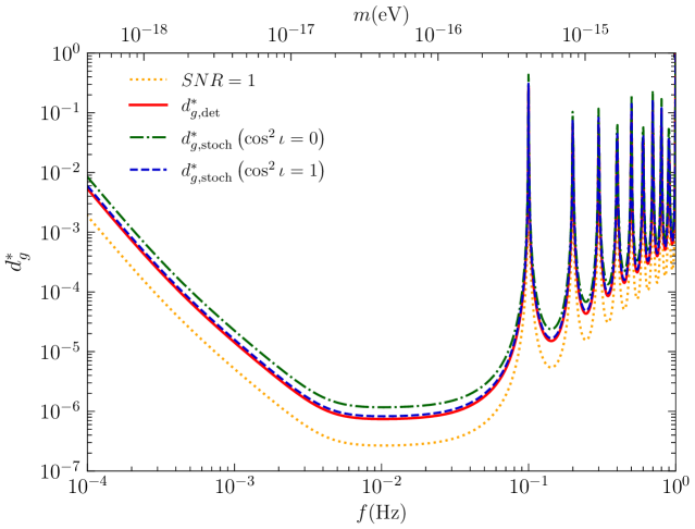
Figure 3: Comparison of sensitivities to the deterministic and stochastic fields, where we present sensitivity curves corresponding to four cases: the stochastic field with the boosted velocity distribution (dash) or isotropic distribution (dot dash), the deterministic field (solid), and the crude $\text{SNR}=1$ estimation (dot). Except for the $\text{SNR}=1$ case, the other three sensitivities correspond to a $95\%$ detection rate and a $5\%$ false alarm rate.

We present the sensitivities of a single detector to the deterministic and stochastic field with a $95\%$ detection rate and a $5\%$ false alarm rate in Fig 3. For illustration purposes, we adopt the parameters of Taiji, which are listed in Appendix B. As depicted in Fig. 3, the minimum value of $d^{*}_{g,\text{det}}$ derived here is greater than that, denote by $\text{SNR}=1$, derived in Yu et al. (2023). This discrepancy arises because the previous sensitivity curve was a rough estimation obtained by setting the signal-to-noise ratio (SNR) equal to one, and it only corresponds to a $22\%$ detection rate for $\alpha=0.05$ within this frequentist formalism. Comparing Eqs. (48, 50), we observe that for $I_{\text{vel}}=I^{\odot}_{\text{vel}}$ and $\cos^{2}\iota=1$, $d^{*}_{g,\text{stoch}}/d^{*}_{g,\text{det}}\approx 1.11$ for $(\alpha,\gamma)=(0.05,0.95)$. Thus, the stochastic effect of ULDM field leads to a mild diminishment in sensitivity.  Although the sensitivities of GW detector to the deterministic and stochastic fields are comparable, it is important to note that the signal models are disparate in the two scenarios, as evidenced by the comparison of Eq. (43) and Eq. (49).

It is pointed out that the stochastic effect will typically relax constraints or sensitivities by a factor ranging from $3$ to $10$ depending on experimental details compared to the deterministic case if the experimens probe the field $\Phi(x)$ directly Centers et al. (2021). We clarify that our results are not in conflict with these findings. In our scenario, a test mass couples with the gradient of the field rather than the field itself. Therefore, the signal, like Michelson interference response Eq. (III.1), involves terms containing $\mathbf{v}\cdot\hat{n}$, and the velocity integral $I_{\text{vel}}$ essentially represents the average of kinetic energy of ULDM particles projected onto the arms of detector. Eq. (33) indicates that the signal power is proportional to the projected kinetic energy of ULDM. Thus, a velocity distribution with a larger projected kinetic energy will yield a stronger signal, which compensates the reduction in sensitivity due to the statistical effect and facilitates probing smaller values of the coupling strength. As illustrated in III.3, the variance of velocity in the isotropic Maxwell distribution is three times larger than that in the $\delta$ distribution. Moreover, in the case of the boosted distribution, the projected kinetic energy receives an additional factor of $2$ enhancement when detector is at an ideal angle with respect to the direction of motion of the solar system, i.e. when detector directly faces the “DM wind”. This also suggests that when using the deterministic field to estimate the sensitivity of experiment which probes the gradient of ULDM field, one can adopt a larger average kinetic energy, such as $3\sigma^{2}$ instead of $\sigma^{2}$, to achieve a more accurate estimation of sensitivity.

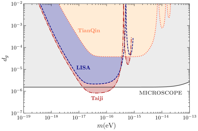
Figure 4: The projected sensitivities of space-based GW detectors with a $95\%$ detection rate and a $5\%$ false alarm rate, where we adopt the boosted velocity distribution and set $\cos^{2}\iota=1$. The $2\sigma$ constraint from the final results of MICROSCOPE et al (2022) is also shown. Note that in this plot we assume that all coupling parameters except $d_{g}$ are zero.

In Fig. 4, we present the projected sensitivities of space-based GW detectors LISA, Taiji and TianQin on $d_{g}$ with a $95\%$ detection rate and a $5\%$ false alaram rate, along with the $2\sigma$ constraint from the final results of MICROSCOPE. The sensitivities correspond to the boosted velocity distribution with $\cos^{2}\iota=1$. The noise parameters adopted for the three GW detectors are summarized in Appendix B. Since GW experiments are sensitive to the composition-independent effect, directly probing $d^{*}_{g}$, while MICROSCOPE are sensitive to the composition-dependent effect, probing a linear combination of $d^{*}_{g}(d_{\tilde{m}}-d_{g})$ and $d^{*}_{g}d_{e}$, we assume that all coupling parameters except $d_{g}$ are zero to ensure a comparison. As illustrated, LISA will approach the constraint given by MICROSCOPE, and Taiji will improve the constraint by a factor of $1.85$ around $4\times 10^{-17}$ eV. Note that the sensitivity is inversely proportional to the square root of the observation time if it is shorter than the coherence time of ULDM, as evident in Eq. (48), and it improves as $T^{1/4}$ if $T>\tau_{c}$ Derevianko (2018); Foster et al. (2018); Nakatsuka et al. (2022). Thus, considering the one-year observation time we used and the potential for longer mission lifetimes, the sensitivities derived here is conservative.

IV.2 Sensitivity of Two-Detector Network

For the specific signals $\tilde{s}_{1}$ and $\tilde{s}_{2}$, the likelihood of data of two detectors with uncorrelated, stationary and Gaussian noise is given by

$$\mathcal{L}\left(\tilde{d}_{1},\tilde{d}_{2}\Big{|}\tilde{s}_{1},\tilde{s}_{2},N_{1}(f),N_{2}(f)\right) =\prod^{n}_{i=1}\frac{1}{\pi TN_{1}(f_{i})}\exp\left[-\frac{\left|\tilde{d}_{1}(f_{i})-\tilde{s}_{1}(f_{i})\right|^{2}}{TN_{1}(f_{i})}\right]$$ (51)

$$\qquad\qquad\quad\times\prod^{n}_{j=1}\frac{1}{\pi TN_{2}(f_{j})}\exp\left[-\frac{\left|\tilde{d}_{2}(f_{j})-\tilde{s}_{2}(f_{j})\right|^{2}}{TN_{2}(f_{j})}\right]$$

where $N_{1}(f)$ and $N_{2}(f)$ are the two-sided noise PSD of detectors, respectively, and the subscripts $i$ and $j$ label the frequency bins. In our scenario, $N_{1}(f)$ and $N_{2}(f)$ correspond to the noise PSD of TDI channels of two space-based GW detectors, like LISA and Taiji. We can write the above likelihood in a more compact form,

$$\mathcal{L}\left(\mathbf{\tilde{d}}\Big{|}\mathbf{\tilde{s}},N_{1},N_{2}\right)=\frac{1}{\det\left[\pi T\mathbf{C}\right]}e^{-(\mathbf{\tilde{d}-\tilde{s}})^{\dagger}(T\mathbf{C})^{-1}(\mathbf{\tilde{d}-\tilde{s}})},$$ (52)

where $\mathbf{\tilde{d}}=[\tilde{d}_{1}(f_{1}),\tilde{d}_{2}(f_{1}),\dots,\tilde{d}_{1}(f_{n}),\tilde{d}_{2}(f_{n})]$, $\mathbf{\tilde{s}}=\left[\tilde{s}_{1}(f_{1}),\tilde{s}_{2}(f_{1}),\dots,\tilde{s}_{1}(f_{n}),\tilde{s}_{2}(f_{n})\right]$, and $\mathbf{C}=\text{diag}\left[N_{1}(f_{1}),N_{2}(f_{1}),\dots,N_{1}(f_{n}),N_{2}(f_{n})\right]$.

Given that the ULDM signal $\tilde{s}_{1}$ and $\tilde{s}_{2}$ are random variables and our interest lies in their statistical characteristics rather than a particular realization, we marginalize over $\mathbf{\tilde{s}}$

$$\mathcal{L}_{\text{stoch}}\left(\mathbf{\tilde{d}}\Big{|}\lambda,S_{\Phi},N_{1},N_{2}\right)=\int d\mathbf{\tilde{s}}\;\mathcal{L}\left(\mathbf{\tilde{d}}\Big{|}\mathbf{\tilde{s}},N_{1},N_{2}\right)\mathcal{L}\left(\mathbf{\tilde{s}}\Big{|}S_{\Phi}\right).$$ (53)

The marginalized likelihood is given by Cornish and Romano (2013)

$$\mathcal{L}_{\text{stoch}}\left(\mathbf{\tilde{d}}\Big{|}\lambda,S_{\Phi},N_{1},N_{2}\right)=\frac{1}{\det[\pi T\mathbf{\Sigma}]}e^{-\mathbf{\tilde{d}}^{\dagger}\left(T\mathbf{\Sigma}\right)^{-1}\mathbf{\tilde{d}}},$$ (54)

where $\mathbf{\Sigma}=\text{diag}\left[\Sigma_{1},\dots,\Sigma_{n}\right]$ is a block diagonal matrix with

$$\Sigma_{i}=\begin{bmatrix}N_{1}(f_{i})&\\ &N_{2}(f_{i})\end{bmatrix}+\lambda^{2}\int d\hat{k}\begin{bmatrix}\chi_{11}(f_{i},\hat{k},v)S_{\Phi}(f_{i},\hat{k})&\;\chi_{12}(f_{i},\hat{k},v)S_{\Phi}(f_{i},\hat{k})\\ \chi_{21}(f_{i},\hat{k},v)S_{\Phi}(f_{i},\hat{k})&\;\chi_{22}(f_{i},\hat{k},v)S_{\Phi}(f_{i},\hat{k})\end{bmatrix},$$ (55)

and

$$\chi_{ab}(f,\hat{k},v):=F_{a}(f,\hat{k},v)F^{*}_{b}(f,\hat{k},v)e^{-i2\pi fv\hat{k}\cdot\Delta\mathbf{x}_{ab}},$$ (56)

where $v$ is the velocity of ULDM particle, $F_{i}(f,\hat{k},v)$ is the response function of the TDI channel $O$ of the $a\textit{th}$ detector, and $\Delta\mathbf{x}_{ab}=\mathbf{x}_{a}-\mathbf{x}_{b}$ with $\mathbf{x}_{a}$ and $\mathbf{x}_{b}$ the position vectors of two detectors, respectively. Given that $v$ is related to $f$ through the dispersion relation of massive particles $v=\sqrt{1-f^{2}_{c}/f^{2}}$, $\chi_{ab}$ can also been viewed as dependent on the mass rather than the velocity of ULDM particle.

Analogous to SGWB detection Allen and Romano (1999); Romano and Cornish (2017), we define the overlap reduction function (ORF) of ULDM as

$$\gamma_{ab}(f,v):=\int d\hat{k}\;\chi_{ab}(f,\hat{k},v),$$ (57)

which quantifies the degree of coherence of ULDM signals observed by two detectors, see Fig. 5. In contrast to the ORF defined in SGWB detection, the ORF of ULDM exhibits velocity dependency (or equivalently mass dependent), arising from both the velocity-dependent response function and the exponential term. Consequently, it becomes necessary to construct a template bank of ORFs for different ULDM masses in the practical searches.

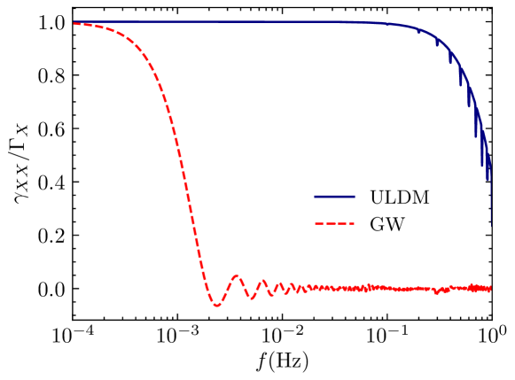
Figure 5: The ratio $\gamma_{ab}(f,v)/\Gamma_{O}(f,v)$ measures the decrease of correlation due to the distance between detectors. The solid line is for ULDM and the dash line is for GWs. Here, we present the ratio for the $X$ channels of a pair of identical detectors with armlength $L=3\times 10^{6}$ km and set $v=\sigma\approx 10^{-3}$. The two detectors are parallel with each other and separated with distance $|\Delta\mathbf{x}_{ab}|=348$ light seconds, corresponding to the configuration in which one detector is leading the Earth at an angle of $20^{\circ}$ and the other is trailing the Earth at an angle of $20^{\circ}$.

As evident from Eq. (55), the marginalization introduces both the auto-correlation of $\tilde{d}_{1}$ and $\tilde{d}_{2}$ as well as the cross-correlation between $\tilde{d}_{1}$ and $\tilde{d}_{2}$, manifesting as additional diagonal and off-diagonal terms in $\Sigma_{i}$, respectively. The strength of cross-correlation is characterized by the ORF and the “sky map” $S_{\Phi}(f,\hat{k})$, akin to SGWB detection. However, unlike the SGWB scenario where the exponential term in Eq. (56) oscillates violently and $\gamma_{ab}(a\neq b)$ decays rapidly when $f>1/|\Delta\mathbf{x}_{ab}|$, the ORF of ULDM will decay when $|\Delta\mathbf{x}_{ab}|>2\pi\lambda_{c}\approx 10^{3}/f_{c}$ due to the longer wavelength of non-relativistic ULDM particles. Therefore, even if two detectors are separated by more than $1/f_{c}$ apart, they will still retain correlation for ULDM detection.

With the above formalism, we can derive the sensitivity of the network in the most general situation. However, in our scenario, things simplify considerably. Since ULDM signal is concentrated within a single frequency bin centered around its Compton frequency, we can safely ignore all other frequency bins containing only noise in the likelihood. Additionally, We assume identical detectors and use a isotropic spectrum $S_{\Phi}(f)$ to streamline our analysis. To simplify notation, we omit the subscript of $f_{c}$ and use $f$ to denote the frequency bin containing the Compton frequency in the following discussion.

We first derive the sensitivity of the network in the co-aligned and co-located configuration, which is the optimal configuration for SGWB detection. In this case, the exponential term in Eq. (56) equals one and the ORFs reduce to the square of modulus of the response function defined in III.2. For the two $X$ channels of detectors, we have

$$\mathbf{\Sigma}=N(f)\begin{bmatrix}1&\\ &1\end{bmatrix}+\lambda^{2}\Gamma_{X}(f)S_{\Phi}(f)\begin{bmatrix}1&1\\ 1&1\end{bmatrix},$$ (58)

where $N(f)\equiv N_{1}(f)=N_{2}(f)$.

We use the maximum likelihood estimator (MLE) of $\lambda^{2}$ as the detection statistic  and denote it by $\hat{\lambda}^{2}$. For a specific data $\mathbf{\tilde{d}}$, $\hat{\lambda}^{2}$ is determined by

$$\frac{\partial\ln\mathcal{L}_{\text{stoch}}}{\partial\lambda^{2}}\Big{|}_{\hat{\lambda}^{2}}=0.$$ (59)

Substitute Eqs. (54, 58) into Eq. $(\ref{ML estimator eq})$, we have

$$4\hat{\lambda}^{2}\cdot\Gamma_{X}S_{\Phi}+2N-\left(\tilde{d}_{1}+\tilde{d}_{2}\right)^{*}\left(\tilde{d}_{1}+\tilde{d}_{2}\right)=0,$$ (60)

or written in terms of the real and imaginary part of $\tilde{d}_{1}$ and $\tilde{d}_{2}$,

$$\hat{\lambda}^{2}=\frac{\left(\Re[\tilde{d}_{1}]+\Re[\tilde{d}_{2}]\right)^{2}+\left(\Im[\tilde{d}_{1}]+\Im[\tilde{d}_{2}]\right)^{2}-2N}{4\Gamma_{X}S_{\Phi}}.$$ (61)

Now we need to derive the probability density function (PDF) of $\hat{\lambda}^{2}$ given the true value of coupling strength $\lambda$. In general, this can only be accomplished numerically through the Monte Carlo simulation. However, due to the specific form of the detection statistic Eq. (61) and the likelihood Eq. (54), we can obtain the pdf of $\hat{\lambda}^{2}$ analytically.

Notice that $\Sigma$ is symmetric and $\Sigma^{-1}$ can be diagonalized through an orthogonal transformation. After diagonalization, the likelihood takes the form,

$$\mathcal{L}_{\text{stoch}}\left(u_{1},u_{2},v_{1},v_{2}\Big{|}\lambda,S_{\Phi},N_{1},N_{2}\right)=\frac{1}{4\pi^{2}}\exp\left(-\frac{u^{2}_{1}+u^{2}_{2}+v^{2}_{1}+v^{2}_{2}}{2}\right),$$ (62)

where the new variables are related to the old ones by

$$u_{1} =\frac{\Re[\tilde{d}_{1}]-\Re[\tilde{d}_{2}]}{\sqrt{N}},\qquad v_{1}=\frac{\Re[\tilde{d}_{1}]+\Re[\tilde{d}_{2}]}{\sqrt{\zeta}},$$ (63)

$$u_{2} =\frac{\Im[\tilde{d}_{1}]-\Im[\tilde{d}_{2}]}{\sqrt{N}},\qquad v_{2}=\frac{\Im[\tilde{d}_{1}]+\Im[\tilde{d}_{2}]}{\sqrt{\zeta}},$$

where $\zeta\equiv 2\lambda^{2}\Gamma_{X}S_{\Phi}+N$. In this new set of variables,

$$\hat{\lambda}^{2}=\frac{\zeta(v_{1}^{2}+v_{2}^{2})-2N}{4\Gamma_{X}S_{\Phi}}.$$ (64)

The term $v_{1}^{2}+v_{2}^{2}$ is the sum of the squares of two independent Gaussian variables with zero mean and unit variance, and it is well known that this sum follows the $\chi^{2}$ distribution with $2$ degrees of freedom. Thus, the pdf of $\hat{\lambda}^{2}$ can be obtained from the $\chi^{2}$ distribution through a variable transformation and the result is

$$\mathcal{L}_{\text{stoch}}\left(\hat{\lambda}^{2}\Big{|}\lambda,S_{\Phi},N_{1},N_{2}\right)=\frac{2\gamma_{X}S_{\Phi}}{\zeta}\exp\left[-\left(\frac{2\gamma_{X}S_{\Phi}}{\zeta}\hat{\lambda}^{2}+\frac{N}{\zeta}\right)\right].$$ (65)

With the PDF of detection statistic in hand, we are now prepared to calculate the sensitivity of the network in the co-aligned and co-located configuration. The minimum value of $\lambda$ that can be detected, with a detection rate $\gamma$ and a false alarm rate $\alpha$, is determined by

$$\alpha =\int^{\infty}_{\hat{\lambda}^{2}_{*}}d\hat{\lambda}^{2}\;\mathcal{L}_{\text{stoch}}\left(\hat{\lambda}^{2}\Big{|}\lambda=0,S_{\Phi},N_{1},N_{2}\right),$$ (66)

$$\gamma =\int^{\infty}_{\hat{\lambda}^{2}_{*}}d\hat{\lambda}^{2}\;\mathcal{L}_{\text{stoch}}\left(\hat{\lambda}^{2}\Big{|}\lambda_{\text{min}},S_{\Phi},N_{1},N_{2}\right).$$ (67)

Substitute Eq. $(\ref{2d optimal lambda dis})$ into Eqs. (66, 67), we have

$$\lambda_{\text{min}}^{2}=\frac{N}{2\Gamma_{X}S_{\Phi}}\left(\frac{\ln\alpha}{\ln\gamma}-1\right).$$ (68)

Comparing with Eq. $(\ref{1d lambda^2})$, we observe a $\sqrt{2}$ improvement in sensitivity for the two-detector network. In general, if there are $n$ co-aligned and co-located identical detectors, we will have $n(n-1)/2$ detector pairs, resulting in a $\sqrt{n(n-1)/2}$ improvement in sensitivity.

This is in sharp contrast with SGWB detection. In SGWB detection, we typically achieve about several orders of magnitude improvement in sensitivity when correlating the outputs of two detectors. It may seem surprising we only have a $\sqrt{2}$ improvement here.

To address this question, it is important to understand why correlation usually can lead to a substantial enhancement in sensitivity in SGWB detection. A key technique employed in the search of deterministic GW signals is matched filtering. In the context of “deterministic”, the signal is uniquely determined by its parameters, which allows us to predict its shape either in the time domain or frequency domain. Leveraging this predicted shape enables us to match it with the detector’s output, thereby greatly improving sensitivity. However, for “stochastic” signals, their shape in a specific realization cannot be predicted even with the knowledge of the parameters determining their statistical properties. To tackle this issue, we require the use of two detectors. With two detectors at our disposal, we can use the output of one detector as the template to match the output of the other detector. This is precisely the correlation technique used in SGWB detection. The picture in the detection of ULDM is different. Although the amplitude of ULDM signal is stochastic, we know it consists of oscillating sine waves with frequency $f_{c}$. Using sine waves with different frequencies as templates, essentially performing the Fourier transform, will filter out the ULDM signal from the data. Therefore, the excess power calculated in IV.1 is already equivalent to matched filtering and the $\sqrt{2}$ improvement in sensitivity when correlating the output of two detectors in ULDM detection corresponds to the $\sqrt{2}$ improvement when optimally combining the measurements of two detector pairs in SGWB detection.

We can also determine the sensitivity in the case where two detectors are widely separated, i.e. $|\Delta\mathbf{x}_{ab}|\gg\lambda_{c}$. In this scenario, the correlation between detectors is negligible and the off-diagonal terms in $\mathbf{\Sigma}$ vanish,

$$\mathbf{\Sigma}=N(f)\begin{bmatrix}1&\\ &1\end{bmatrix}+\lambda^{2}\Gamma_{X}(f)S_{\Phi}(f)\begin{bmatrix}1&\\ &1\end{bmatrix}=\left(N+\lambda^{2}\Gamma_{X}S_{\Phi}\right)I_{2\times 2},$$ (69)

and the likelihood reduces to

$$\mathcal{L}_{\text{stoch}}\left(\mathbf{\tilde{d}}\Big{|}\lambda,S_{\Phi},N_{1},N_{2}\right)=\frac{1}{\pi^{2}\left(N+\lambda^{2}\Gamma_{X}S_{\Phi}\right)^{2}}\exp\left(-\frac{\mathbf{\tilde{d}}^{\dagger}\mathbf{\tilde{d}}}{N+\lambda^{2}\Gamma_{X}S_{\Phi}}\right).$$ (70)

Solving Eq. (59), the MLE of $\lambda^{2}$ is given by

$$\hat{\lambda}^{2}=\frac{\mathbf{\tilde{d}}^{\dagger}\mathbf{\tilde{d}}-2N}{2\Gamma_{X}S_{\Phi}}=\frac{\Re[\tilde{d}_{1}]^{2}+\Im[\tilde{d}_{1}]^{2}+\Re[\tilde{d}_{2}]^{2}+\Im[\tilde{d}_{2}]^{2}-2N}{2\Gamma_{X}S_{\Phi}}.$$ (71)

According to Eq. (70), $\Re[\tilde{d}_{1}],\Im[\tilde{d}_{1}],\Re[\tilde{d}_{2}],\Im[\tilde{d}_{2}]$ are independent Gaussian variables with zero mean and variance $\varsigma=(N+\lambda^{2}\Gamma_{X}S_{\Phi})/2$. Therefore, the PDF of $\hat{\lambda}^{2}$ is linked to the $\chi^{2}$ distribution with $4$ degrees of freedom and can be obtained through a variable transformation. The result is

$$\mathcal{L}_{\text{stoch}}\left(\hat{\lambda}^{2}\Big{|}\lambda,S_{\Phi},N_{1},N_{2}\right)=\frac{\Gamma_{X}S_{\Phi}}{\varsigma}\left(\frac{\Gamma_{X}S_{\Phi}}{\varsigma}\hat{\lambda}^{2}+\frac{N}{\varsigma}\right)\exp\left[-\left(\frac{\Gamma_{X}S_{\Phi}}{\varsigma}\hat{\lambda}^{2}+\frac{N}{\varsigma}\right)\right].$$ (72)

Substitute Eq. (72) into Eqs. (66, 67), we obtain the sensitivity of the well-separated configuration

$$\lambda_{\text{min}}^{2}=\frac{N}{\Gamma_{X}S_{\Phi}}\left(\frac{x_{\alpha}}{x_{\gamma}}-1\right)=\frac{N}{G(\alpha,\gamma)\Gamma_{X}S_{\Phi}}\left(\frac{\ln\alpha}{\ln\gamma}-1\right),$$ (73)

where $x_{z}$ is determined by

$$z=\int^{\infty}_{x_{z}}dx\;p_{4}(x)$$ (74)

with $p_{4}(x)$ the PDF of $\chi^{2}$ distribution with $4$ degrees of freedom. The ratio $G(\alpha,\gamma)=(\ln\alpha/\ln\gamma-1)/(x_{\alpha}/x_{\gamma}-1)$ quantifies the relative sensitivity between the two configurations. For $(\alpha,\gamma)=(0.05,0.95)$, $G$ equals $4.64$, surpassing  the $2$ appearing in Eq. (68). This implies that somehow the sensitivity given by the non-correlated configuration is better. This contradicts the intuition derived from SGWB detection, where sensitivity generally benefits from correlation. However, as we will elucidate, this apparent contradiction can be resolved by considering the physical rationale behind preferring a non-correlated network in ULDM detection.

We go back to Eq. $(\ref{1d power ratio})$, which indicates the relative strength between the ULDM signal and the detector noise. For $(\alpha,\gamma)=(0.05,0.95)$, we observe that the minimum detectable value of $d^{*}_{g}$ corresponds to a power of signal that is $57$ times greater than that of noise. Even when using a two-detector network, which improves the sensitivity by a factor of $\mathcal{O}(1)$, the signal power remains notably higher than the noise power by an order of magnitude. In summary, we are seeking for a relatively strong signal within the detector data, and the noise is not a serious obstacle to signal detection. Thus, as evidenced by the mere $\sqrt{2}$ enhancement, while correlation can help in discriminating the signal from the noise, the extent of improvement in sensitivity is limited. This differs from SGWB detection, where a weak signal is buried in the noise and correlation boosts sensitivity significantly.

While utilizing correlation to suppressing the noise is not so substantial, there is a significant advantage for ULDM detection when two detectors are widely separated. In the co-aligned and co-located configuration, detectors sample a single patch of the field. This setup can lead to weak signals simultaneously if the amplitude of the field in the patch is close to zero due to fluctuation, even if the coupling strength $d^{*}_{g}$ is not small. On the contrast, when detectors are separated by a distance greater than the coherence length of ULDM, they will probe two patches with uncorrelated amplitudes, as illustrated in Fig. 1. This reduces the likelihood that both detectors meet a small amplitude and have weak signals simultaneously. Therefore, the well-separated configuration has a lower chance of missing ULDM signal compared to the co-aligned and co-located configuration.

The sensitivity gains from the less chance of missing compete with the loss resulting from the absence of correlation. Since we hope to detect ULDM signal with a high probability under a low false alarm rate, which corresponds to a strong signal, “the less chance of missing” is more crucial, and the well-separated configuration is preferred.

IV.3 Discriminate ULDM Signal From Monochromatic GWs

As elaborated in the preceding sections, ULDM will manifest as a characteristic sinusoidal oscillation in space-based GW interferometers. However, within the detector’s frequency band, there are also other monochromatic signals, such as gravitational waves from galactic white dwarf binaries (WDBs) Sathyaprakash and Schutz (2009). This raises the question: How can we distinguish between a monochromatic signal originating from ULDM and one from WDBs?

One potential approach involves leveraging the distinct responses of TDI channels to ULDM and GWs. As shown in Yu et al. (2023), while the $X$ channel exhibits similar responses to ULDM and GWs throughout the frequency band, the Sagnac combination $\zeta$ shows a weaker response to ULDM compared to GWs. Therefore, the ratio between the SNR of ULDM signal measured in the $\zeta$ channel and that measured in the $X$ channel will be smaller than the corresponding ratio of GWs.

Another distinguishing factor between ULDM signal and the GWs from WDBs lies in their spatial characteristics. Since space-based GW detectors primarily search for WDBs in the Milky Way, the GWs emitted by these sources predominantly emanate from the direction of the galactic disk. On the contrary, the direction of ULDM field’s gradient is random. In an isotropic halo, the probability density function of the gradient’s direction vector is uniform across the celestial sphere and there is a considerable probability that the direction vector does not align with the galactic disk. Therefore, if a monochromatic signal is detected and subsequent parameter estimation reveals that its sky location does not lie in the galactic disk, then it becomes more plausible that the signal originates from ULDM rather than WDB.

Finally, if the network composed of detectors spaced farther apart than the coherence length of ULDM, the stochastic nature of ULDM field’s amplitude may also aid in distinguishing it from GWs. In such a scenario, each detector will sample a distinct patch of the field independently and the field amplitudes in these patches are uncorrelated. Consequently, the SNRs of ULDM measured by individual detectors may be quite different. For instance, if one detector is positioned in a patch with a large field amplitude, while the other unfortunately in a patch with a small field amplitude, then the former is likely to report a significantly higher SNR compared to the latter. However, such disparity in SNR is less likely to occur for GWs, where separated detectors are more likely to report SNRs of similar magnitudes, given that detectors have comparable noise levels.

V Conclusions

In this work, we investigate the sensitivity of space-based gravitational-wave detectors to the stochastic ultralight dark matter field and illustrate with the model in which the test masses are coupled with the gradient of scalar ULDM field. We find that the sensitivity is only mildly affected by the stochastic effect. This differs from the searches concerning direct coupling with the field itself, where the stochastic effect reduces the sensitivity significantly. Future missions, such as LISA and Taiji, are projected to improve the current best limit from MICROSCOPE, up to a factor of two around the most sensitive mass range $\sim 10^{-17}~{}$eV with a one-year observation. Since the sensitivity is inversely proportional to the square root of observation time, tighter constraints are probable, considering the potentially longer lifetimes of missions. We also find that GW experiments are sensitive to the composition-independent effect of ULDM, making them complementary to the composition-dependent experiments like EP tests.

We further explore the sensitivity of two-detector network by applying the general correlation likelihood to ULDM detection. We introduce the overlap reduction function for ULDM, which measures the correlation of ULDM signals between detectors. We analytically derive the sensitivity of the network in two typical configurations and find that the well-separated configuration, where the distance between two detectors exceeds the coherence length of ULDM, outperforms the co-located and co-aligned setup in ULDM detection. In the well-separated configuration, detectors probe independent patches of the ULDM field, reducing the probability that all patches have negligible amplitudes and increasing the chance of detecting a signal. Our findings provide new insights for potential joint observations involving space-based detectors like LISA and Taiji.

Appendix A Derivation of the two-point correlation function

We present a detailed derivation of the two-point correlation function presented in II. The two-point correlation function is defined as

$$\begin{split}\left\langle\Phi(x)\Phi(x^{\prime})\right\rangle&=\frac{\rho}{m^{2}}\left\langle\sum_{n,l}\sqrt{\Delta_{nl}}\beta_{nl}\cos\left[m\left(1+\frac{v_{n}^{2}}{2}\right)t-\mathbf{k}_{nl}\cdot\mathbf{x}+\theta_{nl}\right]\right.\\ &\qquad\qquad\left.\times\sum_{p,q}\sqrt{\Delta_{pq}}\beta_{pq}\cos\left[m\left(1+\frac{v_{p}^{2}}{2}\right)t^{\prime}-\mathbf{k}_{pq}\cdot\mathbf{x}^{\prime}+\theta_{pq}\right]\right\rangle.\end{split}$$ (75)

We split the sum over $n$, $l$, $p$, $q$ into the diagonal part $(n,l)=(p,q)$ and the off-diagonal part $(n,l)\neq(p,q)$. For the diagonal part,

$$\begin{split}&\sum_{n,l}\Delta_{nl}\times\left\langle\beta^{2}_{nl}\right\rangle\times\left\langle\cos\left[m\left(1+\frac{v_{n}^{2}}{2}\right)t-\mathbf{k}_{nl}\cdot\mathbf{x}+\theta_{nl}\right]\right.\\ &\qquad\qquad\qquad\qquad\qquad\left.\cos\left[m\left(1+\frac{v_{n}^{2}}{2}\right)t^{\prime}-\mathbf{k}_{nl}\cdot\mathbf{x}^{\prime}+\theta_{nl}\right]\right\rangle\\ &=\sum_{n,l}\Delta_{nl}\times 2\times\frac{1}{2}\cos\left[m\left(1+\frac{v_{n}^{2}}{2}\right)\tau-\mathbf{k}_{nl}\cdot\mathbf{d}\right],\end{split}$$ (76)

where $\tau=t^{\prime}-t$ and $\mathbf{d}=\mathbf{x}^{\prime}-\mathbf{x}$, and we use $\left\langle\beta^{2}_{nl}\right\rangle=2$. The average of the product of two $\cos$ functions can be evaluated with the help of

$$\left\langle\cos(x+\theta)\cos(y+\theta)\right\rangle=\int^{2\pi}_{0}\frac{d\theta}{2\pi}\cos(x+\theta)\cos(y+\theta)=\frac{1}{2}\cos(y-x).$$

For the off-diagonal part,

$$\sum_{(n,l)\neq(p,q)}\sqrt{\Delta_{nl}\Delta_{pq}}\times\left\langle\beta_{nl}\right\rangle\left\langle\beta_{pq}\right\rangle\times\left\langle\cos\left[m\left(1+\frac{v_{n}^{2}}{2}\right)t-\mathbf{k}_{nl}\cdot\mathbf{x}+\theta_{nl}\right]\right\rangle\times\left\langle\cdots\right\rangle.$$ (77)

The average of a single $\cos$ function gives zero. Thus, the off-diagonal part does not contribute to the two-point correlation function. Collecting the above results, we have

$$\left\langle\Phi(x)\Phi(x^{\prime})\right\rangle=\frac{\rho}{m^{2}}\sum_{n,l}\Delta_{nl}\times\cos\left[m\left(1+\frac{v_{n}^{2}}{2}\right)\tau-\mathbf{k}_{nl}\cdot\mathbf{d}\right],$$ (78)

or written in the continuous form

$$\left\langle\Phi(x)\Phi(x^{\prime})\right\rangle=\frac{\rho}{m^{2}}\int d^{3}v\;f(\mathbf{v})\cos\left[m\left(1+\frac{v^{2}}{2}\right)\tau-\mathbf{k}\cdot\mathbf{d}\right].$$ (79)

Appendix B The power spectral density of noise

The one-sided power spectral density of noise in $X$ channel is given by

$$N_{X}=16\sin^{2}(2\pi fL)\left\{\left[3+\cos(4\pi fL)\right]S_{\text{acc}}+S_{\text{oms}}\right\},$$ (80)

where $L$ is the armlength of interferometer, and $S_{\text{oms}}$ and $S_{\text{acc}}$ stand for the optical metrology system noise and test mass acceleration noise, respectively. They are further described as

$$S_{\text{oms}}\left(f\right) =\left(\frac{2\pi f}{c}s_{\text{oms}}\right)^{2}\left[1+\left(\frac{2\times 10^{-3}~{}\textrm{Hz}}{f}\right)^{4}\right]\;\frac{1}{\textrm{Hz}},$$ (81)

$$S_{\text{acc}}\left(f\right) =\left(\frac{s_{\text{acc}}}{2\pi fc}\right)^{2}\left[1+\left(\frac{0.4\times 10^{-3}~{}\textrm{Hz}}{f}\right)^{2}\right]\;\left[1+\left(\frac{f}{8\times 10^{-3}~{}\textrm{Hz}}\right)^{4}\right]\;\frac{1}{\textrm{Hz}},$$ (82)

where we adopt the following parameters for LISA et al (2017), Taiji Hu and Wu (2017) and TianQin Luo et al. (2016):

$$\textrm{LISA}:s_{\text{oms}} =15\times 10^{-12}~{}\textrm{m},\; s_{\text{acc}} =3\times 10^{-15}~{}\textrm{m}/\textrm{s}^{2},\; L =2.5\times 10^{6}~{}\textrm{km};$$

$$\textrm{Taiji}:s_{\text{oms}} =8\times 10^{-12}~{}\textrm{m},\; s_{\text{acc}} =3\times 10^{-15}~{}\textrm{m}/\textrm{s}^{2},\; L =3\times 10^{6}~{}\textrm{km};$$

$$\textrm{TianQin}:s_{\text{oms}} =1\times 10^{-12}~{}\textrm{m},\; s_{\text{acc}} =1\times 10^{-15}~{}\textrm{m}/\textrm{s}^{2},\; L =1.7\times 10^{5}~{}\textrm{km}.$$

Appendix C Derivation of the “sky map” of ULDM

Using the plane-wave expansion, we write $\Phi(x)$ as

$$\Phi(x)=\int^{\infty}_{-\infty}df\int d\hat{k}\;\Phi(f,\hat{k})e^{i2\pi f\left(t-\eta\hat{k}\cdot\mathbf{x}\right)},$$ (83)

where $\eta=\sqrt{1-f^{2}_{c}/f^{2}}$ and the integral $\int^{\infty}_{-\infty}df$ should be understood as $\int^{\infty}_{f_{c}}df+\int^{-f_{c}}_{-\infty}df$. Since $\Phi(x)$ is real, we have $\Phi(f,\hat{k})=\Phi^{*}(-f,\hat{k})$. The two-sided power spectral density $S_{\Phi}(f,\hat{k})$ is defined as

$$\left\langle\Phi^{*}(f,\hat{k})\Phi(f^{\prime},\hat{k}^{\prime})\right\rangle=\delta\left(f-f^{\prime}\right)\;\delta^{2}\left(\hat{k},\hat{k}^{\prime}\right)\times S_{\Phi}(f,\hat{k}),$$ (84)

which quantifies the power of ULDM concentrated in the infinitesimal interval $dfd\hat{k}$ centered at frequency $f$ and sky direction $\hat{k}$.

We can recalculate the two-point correlation function using Eqs. (83, 84)

$$\left\langle\Phi(x)\Phi(x^{\prime})\right\rangle =\left\langle\int^{\infty}_{-\infty}df\int d\hat{k}\;\Phi^{*}(f,\hat{k})e^{-i2\pi f\left(t-\eta\hat{k}\cdot\mathbf{x}\right)}\right.$$ (85)

$$\qquad\qquad\qquad\qquad\qquad\qquad\left.\times\int^{\infty}_{-\infty}df^{\prime}\int d\hat{k}^{\prime}\;\Phi(f^{\prime},\hat{k}^{\prime})e^{i2\pi f^{\prime}\left(t^{\prime}-\eta^{\prime}\hat{k}^{\prime}\cdot\mathbf{x}^{\prime}\right)}\right\rangle$$

$$=\int dfdf^{\prime}\int d\hat{k}d\hat{k}^{\prime}\;e^{-i2\pi f\left(t-\eta\hat{k}\cdot\mathbf{x}\right)}e^{i2\pi f^{\prime}\left(t^{\prime}-\eta^{\prime}\hat{k}^{\prime}\cdot\mathbf{x}^{\prime}\right)}$$

$$\qquad\qquad\qquad\qquad\qquad\qquad\times\delta\left(f-f^{\prime}\right)\;\delta^{2}\left(\hat{k},\hat{k}^{\prime}\right)\times S_{\Phi}(f,\hat{k})$$

$$=\int^{\infty}_{-\infty}df\int d\hat{k}\;e^{i2\pi f\left(\tau-\eta\hat{k}\cdot\mathbf{d}\right)}\times S_{\Phi}(f,\hat{k})$$

$$=2\int^{\infty}_{f_{c}}df\int d\hat{k}\;\cos\left(2\pi f\tau-\mathbf{k}\cdot\mathbf{d}\right)\times S_{\Phi}(f,\hat{k})\;,$$

where we use $S_{\Phi}(f,\hat{k})=S_{\Phi}(-f,\hat{k})$ in the last line. The two-point correlation derived in Appendix A can be recast into

$$\left\langle\Phi(x)\Phi(x^{\prime})\right\rangle =\frac{\rho}{m^{2}}\int\frac{d^{3}k}{m^{3}}\;\cos\left(2\pi f\tau-\mathbf{k}\cdot\mathbf{d}\right)f\left(\frac{\mathbf{k}}{m}\right)$$ (86)

$$=\int^{\infty}_{f_{c}}df\int d\hat{k}\;\cos\left(2\pi f\tau-\mathbf{k}\cdot\mathbf{d}\right)\times\frac{2\pi\rho v_{f}}{m^{3}}f(v_{f}\hat{k})\;,$$

where $v_{f}=\sqrt{2(f/f_{c}-1)}$, and we use the non-relativistic approximation $2\pi f\simeq m(1+v^{2}/2)$ and $\mathbf{k}=m\mathbf{v}$. Comparing Eq. (85) with Eq. (86), we have

$$S_{\Phi}(f,\hat{k})=\frac{\pi\rho v_{f}}{m^{3}}f(v_{f}\hat{k}).$$ (87)

References

- Peccei and Quinn (1977) R. D. Peccei and H. R. Quinn, Phys. Rev. Lett. 38, 1440 (1977).
- Weinberg (1978) S. Weinberg, Phys. Rev. Lett. 40, 223 (1978).
- Wilczek (1978) F. Wilczek, Phys. Rev. Lett. 40, 279 (1978).
- Preskill et al. (1983) J. Preskill, M. B. Wise, and F. Wilczek, Physics Letters B 120, 127 (1983).
- Abbott and Sikivie (1983) L. F. Abbott and P. Sikivie, Phys. Lett. B 120, 133 (1983).
- Dine and Fischler (1983) M. Dine and W. Fischler, Phys. Lett. B 120, 137 (1983).
- Damour and Polyakov (1994a) T. Damour and A. M. Polyakov, Gen. Rel. Grav. 26, 1171 (1994a), arXiv:gr-qc/9411069 .
- Damour and Polyakov (1994b) T. Damour and A. M. Polyakov, Nucl. Phys. B 423, 532 (1994b), arXiv:hep-th/9401069 .
- Capozziello and De Laurentis (2011) S. Capozziello and M. De Laurentis, Phys. Rept. 509, 167 (2011), arXiv:1108.6266 [gr-qc] .
- Nelson and Scholtz (2011) A. E. Nelson and J. Scholtz, Phys. Rev. D 84, 103501 (2011).
- Graham et al. (2016) P. W. Graham, J. Mardon, and S. Rajendran, Phys. Rev. D 93, 103520 (2016).
- Ema et al. (2019) Y. Ema, K. Nakayama, and Y. Tang, JHEP 07, 060 (2019), arXiv:1903.10973 [hep-ph] .
- Ahmed et al. (2020) A. Ahmed, B. Grzadkowski, and A. Socha, JHEP 08, 059 (2020), arXiv:2005.01766 [hep-ph] .
- Kolb and Long (2021) E. W. Kolb and A. J. Long, JHEP 03, 283 (2021), arXiv:2009.03828 [astro-ph.CO] .
- de Blok (2010) W. J. G. de Blok, Adv. Astron. 2010, 789293 (2010), arXiv:0910.3538 [astro-ph.CO] .
- Boylan-Kolchin et al. (2011) M. Boylan-Kolchin, J. S. Bullock, and M. Kaplinghat, Mon. Not. Roy. Astron. Soc. 415, L40 (2011), arXiv:1103.0007 [astro-ph.CO] .
- Bullock and Boylan-Kolchin (2017) J. S. Bullock and M. Boylan-Kolchin, Ann. Rev. Astron. Astrophys. 55, 343 (2017), arXiv:1707.04256 [astro-ph.CO] .
- Tulin and Yu (2018) S. Tulin and H.-B. Yu, Phys. Rept. 730, 1 (2018), arXiv:1705.02358 [hep-ph] .
- Hu et al. (2000) W. Hu, R. Barkana, and A. Gruzinov, Phys. Rev. Lett. 85, 1158 (2000).
- Hui et al. (2017) L. Hui, J. P. Ostriker, S. Tremaine, and E. Witten, Phys. Rev. D 95, 043541 (2017).
- Hui (2021) L. Hui, Ann. Rev. Astron. Astrophys. 59, 247 (2021), arXiv:2101.11735 [astro-ph.CO] .
- Derevianko (2018) A. Derevianko, Phys. Rev. A 97, 042506 (2018).
- Foster et al. (2018) J. W. Foster, N. L. Rodd, and B. R. Safdi, Phys. Rev. D 97, 123006 (2018).
- Foster et al. (2021) J. W. Foster, Y. Kahn, R. Nguyen, N. L. Rodd, and B. R. Safdi, Phys. Rev. D 103, 076018 (2021).
- Van Tilburg et al. (2015) K. Van Tilburg, N. Leefer, L. Bougas, and D. Budker, Phys. Rev. Lett. 115, 011802 (2015).
- Arvanitaki et al. (2016) A. Arvanitaki, S. Dimopoulos, and K. Van Tilburg, Phys. Rev. Lett. 116, 031102 (2016).
- Hees et al. (2016) A. Hees, J. Guéna, M. Abgrall, S. Bize, and P. Wolf, Phys. Rev. Lett. 117, 061301 (2016).
- Geraci et al. (2019) A. A. Geraci, C. Bradley, D. Gao, J. Weinstein, and A. Derevianko, Phys. Rev. Lett. 123, 031304 (2019).
- Hochberg et al. (2016) Y. Hochberg, T. Lin, and K. M. Zurek, Phys. Rev. D 94, 015019 (2016).
- Fayet (2018) P. Fayet, Phys. Rev. D 97, 055039 (2018).
- Xia et al. (2021) C. Xia, Y.-H. Xu, and Y.-F. Zhou, Nuclear Physics B 969, 115470 (2021).
- An et al. (2023) H. An, S. Ge, W.-Q. Guo, X. Huang, J. Liu, and Z. Lu, Phys. Rev. Lett. 130, 181001 (2023).
- An et al. (2021) H. An, F. P. Huang, J. Liu, and W. Xue, Phys. Rev. Lett. 126, 181102 (2021).
- Rogers and Peiris (2021) K. K. Rogers and H. V. Peiris, Phys. Rev. Lett. 126, 071302 (2021).
- Fedderke and Mathur (2023) M. A. Fedderke and A. Mathur, Phys. Rev. D 107, 043004 (2023).
- Arvanitaki and Dubovsky (2011) A. Arvanitaki and S. Dubovsky, Phys. Rev. D 83, 044026 (2011).
- Cardoso et al. (2018) V. Cardoso, Óscar J.C. Dias, G. S. Hartnett, M. Middleton, P. Pani, and J. E. Santos, Journal of Cosmology and Astroparticle Physics 2018, 043 (2018).
- Davoudiasl and Denton (2019) H. Davoudiasl and P. B. Denton, Phys. Rev. Lett. 123, 021102 (2019).
- Chen et al. (2020) Y. Chen, J. Shu, X. Xue, Q. Yuan, and Y. Zhao, Phys. Rev. Lett. 124, 061102 (2020).
- Liang et al. (2023) D. Liang, R. Xu, Z.-F. Mai, and L. Shao, Phys. Rev. D 107, 044053 (2023).
- Kim (2023) H. Kim, JCAP 12, 018 (2023), arXiv:2306.13348 [hep-ph] .
- Khmelnitsky and Rubakov (2014) A. Khmelnitsky and V. Rubakov, Journal of Cosmology and Astroparticle Physics 2014, 019 (2014).
- Wu et al. (2023) Y.-M. Wu, Z.-C. Chen, and Q.-G. Huang, JCAP 09, 021 (2023), arXiv:2305.08091 [hep-ph] .
- Sun et al. (2022) S. Sun, X.-Y. Yang, and Y.-L. Zhang, Phys. Rev. D 106, 066006 (2022).
- Cao and Tang (2023) Y. Cao and Y. Tang, Phys. Rev. D 108, 123017 (2023).
- Kim and Mitridate (2024) H. Kim and A. Mitridate, Phys. Rev. D 109, 055017 (2024).
- Luu et al. (2024) H. N. Luu, T. Liu, J. Ren, T. Broadhurst, R. Yang, J.-S. Wang, and Z. Xie, The Astrophysical Journal Letters 963, L46 (2024).
- Adelberger et al. (2003) E. Adelberger, B. Heckel, and A. Nelson, Annual Review of Nuclear and Particle Science 53, 77 (2003), https://doi.org/10.1146/annurev.nucl.53.041002.110503 .
- Damour and Donoghue (2010) T. Damour and J. F. Donoghue, Phys. Rev. D 82, 084033 (2010).
- Williams et al. (2004) J. G. Williams, S. G. Turyshev, and D. H. Boggs, Phys. Rev. Lett. 93, 261101 (2004).
- WILLIAMS et al. (2009) J. G. WILLIAMS, S. G. TURYSHEV, and D. H. BOGGS, International Journal of Modern Physics D 18, 1129 (2009), https://doi.org/10.1142/S021827180901500X .
- Schlamminger et al. (2008) S. Schlamminger, K.-Y. Choi, T. A. Wagner, J. H. Gundlach, and E. G. Adelberger, Phys. Rev. Lett. 100, 041101 (2008).
- Wagner et al. (2012) T. A. Wagner, S. Schlamminger, J. H. Gundlach, and E. G. Adelberger, Classical and Quantum Gravity 29, 184002 (2012).
- et al. (2017) P. T. et al. (MICROSCOPE Collaboration), Phys. Rev. Lett. 119, 231101 (2017).
- et al (2022) P. T. et al (MICROSCOPE Collaboration), Phys. Rev. Lett. 129, 121102 (2022).
- Arvanitaki et al. (2018) A. Arvanitaki, P. W. Graham, J. M. Hogan, S. Rajendran, and K. Van Tilburg, Phys. Rev. D 97, 075020 (2018), arXiv:1606.04541 [hep-ph] .
- Pierce et al. (2018) A. Pierce, K. Riles, and Y. Zhao, Phys. Rev. Lett. 121, 061102 (2018).
- Grote and Stadnik (2019) H. Grote and Y. V. Stadnik, Phys. Rev. Res. 1, 033187 (2019), arXiv:1906.06193 [astro-ph.IM] .
- Vermeulen et al. (2021) S. M. Vermeulen et al., Nature 600, 424 (2021), arXiv:2103.03783 [gr-qc] .
- Abbott et al. (2016) B. P. Abbott et al. (LIGO Scientific, Virgo), Phys. Rev. Lett. 116, 061102 (2016), arXiv:1602.03837 [gr-qc] .
- et al (2018) M. A. et al, Phys. Rev. Lett. 120, 061101 (2018).
- Guo et al. (2019) H.-K. Guo, K. Riles, F.-W. Yang, and Y. Zhao, Commun. Phys. 2, 155 (2019), arXiv:1905.04316 [hep-ph] .
- Fukusumi et al. (2023) K. Fukusumi, S. Morisaki, and T. Suyama, (2023), arXiv:2303.13088 [hep-ph] .
- Miller and Mendes (2023) A. L. Miller and L. Mendes, Phys. Rev. D 107, 063015 (2023).
- et al (2017) P. A.-S. et al, “Laser interferometer space antenna,” (2017), arXiv:1702.00786 [astro-ph.IM] .
- Hu and Wu (2017) W.-R. Hu and Y.-L. Wu, Natl. Sci. Rev. 4, 685 (2017).
- Luo et al. (2016) J. Luo, L.-S. Chen, H.-Z. Duan, Y.-G. Gong, S. Hu, J. Ji, Q. Liu, J. Mei, V. Milyukov, M. Sazhin, C.-G. Shao, V. T. Toth, H.-B. Tu, Y. Wang, Y. Wang, H.-C. Yeh, M.-S. Zhan, Y. Zhang, V. Zharov, and Z.-B. Zhou, Classical and Quantum Gravity 33, 035010 (2016).
- Morisaki and Suyama (2019) S. Morisaki and T. Suyama, Phys. Rev. D 100, 123512 (2019).
- Yu et al. (2023) J.-C. Yu, Y.-H. Yao, Y. Tang, and Y.-L. Wu, Phys. Rev. D 108, 083007 (2023).
- Bergé et al. (2018) J. Bergé, P. Brax, G. Métris, M. Pernot-Borràs, P. Touboul, and J.-P. Uzan, Phys. Rev. Lett. 120, 141101 (2018).
- Centers et al. (2021) G. P. Centers et al., Nature Commun. 12, 7321 (2021), arXiv:1905.13650 [astro-ph.CO] .
- Lisanti et al. (2021) M. Lisanti, M. Moschella, and W. Terrano, Phys. Rev. D 104, 055037 (2021).
- Armstrong et al. (1999) J. W. Armstrong, F. B. Estabrook, and M. Tinto, The Astrophysical Journal 527, 814 (1999).
- Estabrook et al. (2000) F. B. Estabrook, M. Tinto, and J. W. Armstrong, Phys. Rev. D 62, 042002 (2000).
- Tinto and Dhurandhar (2021) M. Tinto and S. V. Dhurandhar, Living Rev. Rel. 24, 1 (2021).
- Allen and Romano (1999) B. Allen and J. D. Romano, Phys. Rev. D 59, 102001 (1999).
- Romano and Cornish (2017) J. D. Romano and N. J. Cornish, Living Rev. Rel. 20, 2 (2017), arXiv:1608.06889 [gr-qc] .
- Gramolin et al. (2022) A. V. Gramolin, A. Wickenbrock, D. Aybas, H. Bekker, D. Budker, G. P. Centers, N. L. Figueroa, D. F. Jackson Kimball, and A. O. Sushkov, Phys. Rev. D 105, 035029 (2022).
- Hui et al. (2021) L. Hui, A. Joyce, M. J. Landry, and X. Li, Journal of Cosmology and Astroparticle Physics 2021, 011 (2021).
- Nakatsuka et al. (2022) H. Nakatsuka, S. Morisaki, T. Fujita, J. Kume, Y. Michimura, K. Nagano, and I. Obata, (2022), arXiv:2205.02960 [astro-ph.CO] .
- Kay (2001) S. M. Kay (Fundamentals Of Statistical Signal Processing, 2001).
- Jaranowski and Krolak (2005) P. Jaranowski and A. Krolak, Living Rev. Rel. 8, 3 (2005), arXiv:0711.1115 [gr-qc] .
- Cornish and Romano (2013) N. J. Cornish and J. D. Romano, Phys. Rev. D 87, 122003 (2013).
- Sathyaprakash and Schutz (2009) B. S. Sathyaprakash and B. F. Schutz, Living Rev. Rel. 12, 2 (2009), arXiv:0903.0338 [gr-qc] .